2.1. Basic equations

In the rotating frame the velocity $\boldsymbol{V}=(v_r,v_{\phi },v_z)$ , written in cylindrical coordinates, and pressure $P$ are governed by the equations

(2.1a) \begin{align} \frac { \partial \boldsymbol{V} }{ \partial t } + (\boldsymbol{V}\boldsymbol{\cdot }\boldsymbol{\nabla })\boldsymbol{V} + 2\boldsymbol{e}_{z}\times \boldsymbol{V} & =-\boldsymbol{\nabla }P+E{\nabla} ^{2}\boldsymbol{V} , \end{align}

(2.1b) \begin{align} \boldsymbol{\nabla }\boldsymbol{\cdot }\boldsymbol{V} & = 0 , \end{align}

where $E$ is the Ekman number, which is defined as $E = \nu /\widehat {\varOmega } \widehat {\rho }_o^{2}$ .

Contrarily to He et al. (Reference He, Favier, Rieutord and Le Dizès2022), which exclusively addressed the linear aspects by omitting the advection term in (2.1a ), this study expands into the nonlinear regime. We consider the following asymptotic expansion of the velocity $\boldsymbol{V}$ and pressure $P$ :

(2.2) \begin{equation} (\boldsymbol{V},P) = \varepsilon (\boldsymbol{v}_1, p_1)\textrm{e}^{-\mathrm{i}\omega t}+ \varepsilon ^2\left [(\boldsymbol{v}_0,p_0)+(\boldsymbol{v}_2,p_2)\textrm{e}^{-2\mathrm{i}\omega t} \right ]+ \mathrm{c}.\mathrm{c}. \end{equation}

Here $\mathrm{c}.\mathrm{c}$ denotes the complex conjugate, $(\boldsymbol{v}_1,p_1)$ is the linear harmonic, $(\boldsymbol{v}_0,p_0)$ is the mean flow correction and $(\boldsymbol{v}_2,p_2)$ is the secondary harmonic velocity. In this paper we focus solely on the mean flow correction.

Three steps are required to compute the mean flow correction. First, similarly to He et al. (Reference He, Favier, Rieutord and Le Dizès2022), the linear response is found by solving

(2.3a) \begin{align} -\mathrm{i}\omega \boldsymbol{v}_1+2\boldsymbol{e}_{z} \times \boldsymbol{v}_1 & =-\boldsymbol{\nabla }p_1+E{\nabla} ^{2} \boldsymbol{v}_1 , \end{align}

(2.3b) \begin{align} \boldsymbol{\nabla }\boldsymbol{\cdot }\boldsymbol{v}_1 & =0 , \end{align}

(2.3c) \begin{align} \quad \boldsymbol{v}_1 & = r\boldsymbol{e}_{\phi } \quad(\text{inner boundary condition}), \end{align}

(2.3d) \begin{align} \quad \boldsymbol{v}_1 & = \boldsymbol{0} \quad(\text{outer boundary condition}). \end{align}

Once the linear harmonic velocity $\boldsymbol{v}_1$ is obtained, the nonlinear terms corresponding to its self-interaction can be calculated at leading order. The resulting Reynolds stresses comprise two parts: the steady forcing and the second harmonic oscillating at $2\omega$ . Throughout this paper, we refer to the divergence of the Reynolds stress tensor (which provides the mean flow forcing) simply as the ‘Reynolds stress’. As the present study focuses on the mean flow, we only consider the steady Reynolds stress $\mathcal{N}_{0}$ ,

(2.4) \begin{equation} \boldsymbol{\mathcal{N}}_{0}=\boldsymbol{v}_1\boldsymbol{\cdot }\boldsymbol{\nabla }\boldsymbol{v}_{1}^{*} + \mathrm{c}.\mathrm{c} , \end{equation}

where $^*$ denotes complex conjugation. The mean flow response $\boldsymbol{v}_0$ corresponds to a perturbation with a zero frequency $\omega =0$ and is governed by the linear forced system

(2.5a) \begin{align} 2\boldsymbol{e}_{z} \times \boldsymbol{v}_{0}+\boldsymbol{\nabla }p_{0} & =-\boldsymbol{\mathcal{N}}_{0}+E {\nabla} ^{2} \boldsymbol{v}_{0} , \end{align}

(2.5b) \begin{align} \boldsymbol{\nabla }\boldsymbol{\cdot }\boldsymbol{v}_0 & =0 , \end{align}

(2.5c) \begin{align} \quad \boldsymbol{v}_0 & =\boldsymbol{0} \quad(\text{inner and outer boundary condition}) , \end{align}

where the forcing $\boldsymbol{\mathcal{N}}_0$ arises from the nonlinear self-interaction of the linear harmonic $v_1$ .

2.2. Numerical approach

To solve the equations outlined in § 2.1 and validate our theoretical predictions through asymptotic analysis, we have employed high-precision spectral methods for the numerical integrations. These methods, previously used in Rieutord & Valdettaro (Reference Rieutord and Valdettaro1997) and He et al. (Reference He, Favier, Rieutord and Le Dizès2022) to solve the linear governing equations (2.3), have enabled us to capture the linear harmonic velocity profiles $\boldsymbol{v}_{1}$ displayed in figure 1(a). We have looked for the solution of the linear governing equation (2.3a ) expressed in vorticity form as

(2.6) \begin{equation} -\mathrm{i}\omega \boldsymbol{\nabla }\times \boldsymbol{v}_1+2\boldsymbol{\nabla }\times (\boldsymbol{e}_z\times \boldsymbol{v}_1)=E\boldsymbol{\nabla }\times ({\nabla} ^{2}\boldsymbol{v}_1) . \end{equation}

For this three-dimensional problem, we use spherical coordinates $(\rho , \theta , \phi )$ representing radial, polar and azimuthal directions, respectively. The velocity fields are expanded using spherical harmonics in the polar and azimuthal directions and Chebyshev polynomials in the radial direction, i.e.

(2.7) \begin{equation} \boldsymbol{v}_{1}=\sum ^{+\infty }_{l=0}\sum ^{+l}_{m=-l}u_{m}^{l}(\rho )\boldsymbol{R}_{l}^{m}+v^{l}_{m}(\rho )\boldsymbol{S}_{l}^{m}+w_{m}^{l}(\rho )\boldsymbol{T}_{l}^{m} , \end{equation}

where

(2.8) \begin{equation} \boldsymbol{R}_{l}^{m}=Y_{l}^{m}(\theta ,\phi )\boldsymbol{e}_{\rho },\qquad \boldsymbol{S}_{l}^{m}=\boldsymbol{\nabla }Y_{l}^{m},\qquad \boldsymbol{T}_{l}^{m}=\boldsymbol{\nabla }\times \boldsymbol{R}_{l}^{m} . \end{equation}

Projecting the vorticity (2.6) onto this basis allows us to solve the linear system using a block tridiagonal algorithm. In our cases, we are assuming an axisymmetric fluid response along with the no-slip boundary conditions on the spherical shell. Detailed descriptions of the numerical methods and the construction of the system are available in He et al. (Reference He, Favier, Rieutord and Le Dizès2022) and He et al. (Reference He, Favier, Rieutord and Le Dizès2023) for readers interested in further details.

After obtaining the linear harmonic response numerically, we apply a pseudo-spectral method to calculate the steady Reynolds stress. Subsequently, we solve the governing equations (2.5) to determine the mean flow velocity, $\boldsymbol{v}_0$ , shown in figure 1(a). The nonlinear vorticity equation for the mean zonal flow is expressed as

(2.9) \begin{equation} 2\boldsymbol{\nabla }\times (\boldsymbol{e}_z\times \boldsymbol{v}_0)=-\boldsymbol{\nabla }\times (\boldsymbol{v}_1\boldsymbol{\cdot }\boldsymbol{\nabla }\boldsymbol{v}_1^{*}+\mathrm{c}.\mathrm{c}) +E \boldsymbol{\nabla }\times {\nabla} ^{2}\boldsymbol{v}_{0} . \end{equation}

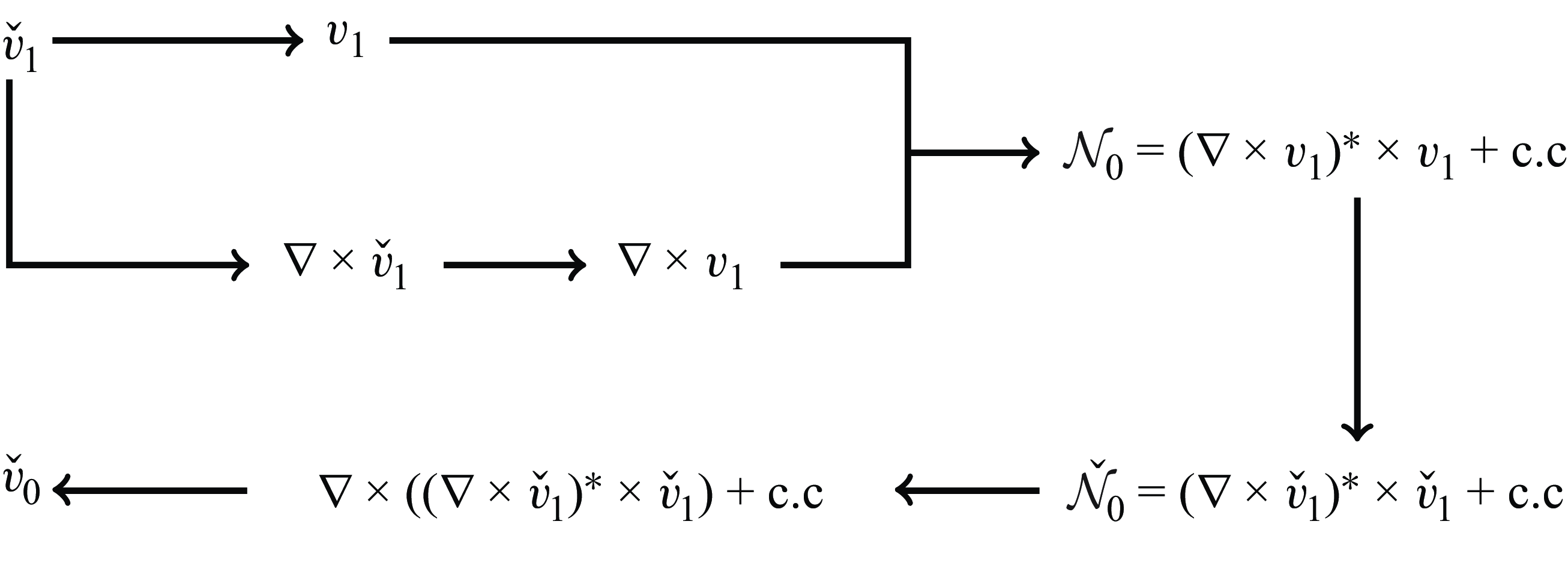
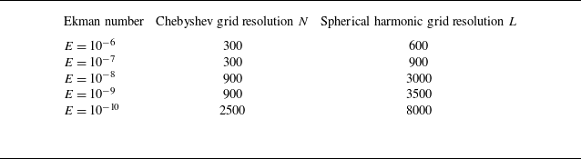
Details on the pseudo-spectral numerical workflow are provided in Appendix A and illustrated in figure 24. We have also investigated potential aliasing issues in this nonlinear set-up and found no significant impact on the results, regardless of whether dealiasing was applied or not. Consequently, all the results discussed in the present paper have not been dealiased. The convergence of our simulations is further demonstrated in Appendix A and the numerical resolutions for different Ekman numbers are documented in table 1 of this appendix. It is important to note that the resolutions required for the nonlinear simulations exceed those used in the purely linear analyses, to ensure similar convergence properties in both cases.

3.1. Self-similar solution and scaling

For the harmonic solution, the localised concentrated beams travel on the beam ray with a constant width of order $E^{1/3}$ . The self-similar beam solution provided by Moore & Saffman (Reference Moore and Saffman1969) was used by Le Dizès & Le Bars (Reference Le Dizès and Le Bars2017) and He et al. (Reference He, Favier, Rieutord and Le Dizès2022) to describe at leading order the velocity $v_{1\parallel }$ along the direction of the beam propagation,

(3.1) \begin{equation} v_{1\parallel }\sim \frac {1}{\sqrt { r }}C_{0}H_{m}(x_{\parallel },x_{\perp })=\frac {1}{\sqrt { r }}C_{0}\left ( \frac {x_{\parallel }}{2\sin \theta } \right )^{-m/3}h_{m}(\zeta ) . \end{equation}

The special function $h_m(\zeta )$ is

(3.2) \begin{equation} h_m(\zeta )=\frac {\text{e}^{-\mathrm{i}m\pi /2}}{(m-1)!}\int _0^{+\infty }\text{e}^{\mathrm{i}p\zeta -p^3}p^{m-1}{\rm d}p , \end{equation}

with the similarity variable,

(3.3) \begin{equation} \zeta =\frac {x_{\perp }}{E^{1/3}}\left ( \frac {2\sin \theta }{x_{\parallel }} \right )^{1/3} . \end{equation}

Here $\theta$ is the angle between the inertial wave propagation direction and the equatorial plane, where $\theta = \pi /4$ enables the formation of a simple closed wave circuit in our configuration (see figure 2 b). This angle also defines the inclination of the internal shear layers relative to the equatorial plane, with the libration frequency $\omega = 2\cos \theta$ . The index $m$ of the function $h_m(\zeta )$ characterises the nature of the singularity that leads to the formation of the beam (Moore & Saffman Reference Moore and Saffman1969; Thomas & Stevenson Reference Thomas and Stevenson1972), while the complex amplitude $C_0$ represents the amplitude of the singularity. A brief review of different values of the index $m$ for various configurations is provided by Le Dizès (Reference Le Dizès2020). In particular, for any axisymmetric convex librating object, such as the inner sphere considered in the present study, Le Dizès & Le Bars (Reference Le Dizès and Le Bars2017) determined the values $m = 5/4$ and $C_0$ by matching the similarity solution with the boundary layer solution around the critical latitude leading to

(3.4a) \begin{align} C_0^N & = E^{1/12}\tilde {C}_{0}^{N}=E^{1/12}\frac {\textrm{e}^{\mathrm{i}\pi /2}}{8(2\sin \theta )^{3/4}} \quad (\text{northward ray}) , \end{align}

(3.4b) \begin{align} C_0^S & =E^{1/12}\tilde {C}_{0}^{S}=E^{1/12}\frac {\textrm{e}^{\mathrm{i}3\pi /4}}{8(2\sin \theta )^{3/4}} \quad (\text{southward ray}) . \end{align}

Expression (3.1) describes the main velocity component. In the $(r,z)$ plane, there also exists a component along $\boldsymbol{e}_\perp$ that is $O(E^{1/3})$ smaller.

As shown by (3.4), the velocity amplitude scales as $E^{1/12}$ in the asymptotic theory. Internal shear layers within a spherical shell were observed to preserve their self-similar structure upon reflecting on boundaries, undergoing either contraction or expansion during this process. Particular attention was given to how these layers propagate along a periodic rectangular path at specific frequencies of the libration forcing (He et al. Reference He, Favier, Rieutord and Le Dizès2022). Additionally, reflections on the rotation axis were found to induce a phase shift, facilitating the convergence of the summation describing the beam superpositions. The final expressions for the velocity components were derived from these self-similar solutions, resulting in the following compact form in the $(r,z)$ plane:

(3.5) \begin{equation} \boldsymbol{v}_{1_{2D}}\sim \frac {E^{1/12}}{\sqrt {r}}(\tilde {C}_{0}^{N}G_{m}(x_{\perp }^{N},x_{\parallel }^{N},L^{N}) \boldsymbol{ e}_{\parallel }^N+\tilde {C}_{0}^{S}G_{m}(x_{\perp }^{S},x_{\parallel }^{S},L^{S})\boldsymbol{e}_{\parallel }^S) . \end{equation}

Here the new function $G_m$ is given by

(3.6a) \begin{align} G_{m}(x_{\perp },x_{\|},L)&=\left ( \frac {x_{\parallel }}{2\sin \theta } \right )^{-m/3}g_{m}(\zeta ,L/x_{\parallel }) , \end{align}

(3.6b) \begin{align} g_{m}(\zeta ,L/x_{\parallel })&=\frac {\textrm{e}^{-\mathrm{i}m\pi /2}}{(m-1)!}\int _0^\infty \frac {\textrm{e}^{\mathrm{i}p\zeta -p^3}p^{m-1}}{1-\mathrm{i}\textrm{e}^{-p^3L/x_{\parallel }}}{\rm d}p , \end{align}

where $L$ is the cumulative propagation distance along the rectangular characteristic path for one cycle (explicit form in Appendix B, (B1)).

Compared to the function $h_m$ in (3.2), the denominator of $g_m$ comes from the beam summation and the ‘ $\mathrm{i}$ ’ factor from the phase shift induced by the reflection on the axis. Note that $\boldsymbol{ e}_{\parallel }^S= -\boldsymbol{e}_{\parallel }^N$ .

Expression (3.5) describes the solution on the rectangular circuit $P_1P_3P_7P_4$ . As explained in He et al. (Reference He, Favier, Rieutord and Le Dizès2022), a weaker secondary beam is also present between $S_c$ and $P_6$ owing to the reflection on the inner core. The width scaling of this secondary beam is $E^{1/6}$ , indicating a relatively larger transverse scale on which viscous diffusion becomes negligible. Consequently, the parallel velocity component $v_{1\parallel }$ of the beam remains constant throughout its path. Furthermore, the amplitude of the beam scales as $E^{1/4}$ , which is significantly smaller than the amplitude of the solution on the main beam. The velocity profile along the beam is asymptotically described by

(3.7) \begin{equation} \boldsymbol{v}_{1_{2D}} \sim \frac {E^{1/4}}{\sqrt {r}}( \tilde {C}_0^{N}\breve {F}_{m}(\breve {x}_{\perp }^N,\lambda ^{N}) \boldsymbol{e}_{\parallel }^N + \tilde {C}_0^{S}\breve {F}_{m}(\breve {x}_{\perp }^S,\lambda ^{S}) \boldsymbol{e}_{\parallel }^S) ,\end{equation}

where

(3.8) \begin{equation} \breve {F}_m(\breve {x}_{\perp },\lambda ) =\frac {\breve {x}_\perp }{\sqrt {2}}\frac {\textrm{e}^{-\mathrm{i}m\pi /2}}{(m-1)!}\int _0^\infty \textrm{e}^{\mathrm{i}p\lambda (\breve {x}_{\perp })^2}\frac {\textrm{e}^{-p^3L/\sqrt {2}}p^{m-1}}{1-\mathrm{i}\textrm{e}^{-p^3L/\sqrt {2}}}{\rm d}p , \end{equation}

with $\lambda ^{N}=-\sqrt {2}/4$ , $\lambda ^{S}=\sqrt {2}/4$ and $\breve {x}_{\perp }=x_\perp /E^{1/6}$ .

A detailed comparison between this asymptotic solution (AS) and numerical solutions (NS) of the linear harmonic viscous problem can be found in He et al. (Reference He, Favier, Rieutord and Le Dizès2022).

The azimuthal velocity, $v_{1\phi }$ , can be readily derived from $v_{1\|}$ using

(3.9) \begin{equation} v_{1\phi }\sim \pm \mathrm{i}v_{1\|} , \end{equation}

where the positive sign (respectively negative sign) corresponds to an obtuse angle (respectively acute angle) between $\boldsymbol{e}_{\parallel }$ and $\boldsymbol{e}_r$ . This equation also implies that, for $\theta =\pi /4$ ,

(3.10) \begin{equation} v_{1\phi }\sim -\sqrt {2}\mathrm{i} v_{1r}. \end{equation}

The velocity field defined by (3.5) and (3.7) also satisfies, for $\theta =\pi /4$ , the remarkable property

(3.11) \begin{equation} \frac {\partial v_{1r} }{\partial z} \sim - \frac {\partial v_{1z} }{\partial r} . \end{equation}

The symbol ` $\sim$ ’ in (3.9), (3.10) and (3.11) has to be understood as denoting equality up to corrections of order $E^{1/3}$ . We shall see below the importance of these equations for simplifying the expression of the Reynolds stress.

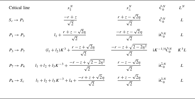
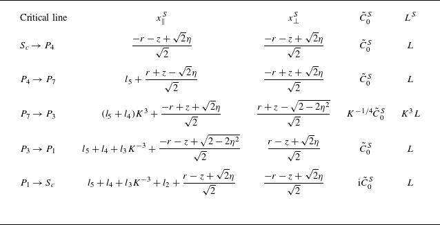
For detailed information about the local coordinate system relationships of northward and southward ray propagation paths, as well as more details about the different beam amplitudes, see tables 2 and 3 in Appendix B. In the following, we shall often keep the parameter $m$ unprescribed to show the dependency of the various expressions with respect to this parameter, but one has to keep in mind that in the present analysis $m$ and $\theta$ are actually fixed to $m=5/4$ and $\theta =\pi /4$ .

Figure 3 illustrates the scaling behaviour derived from the linear part of the asymptotic analysis. In this figure the beam width scalings are shown in red, while the amplitude scalings are depicted in blue. In particular, the main beam is characterised by a beam width scaling like $E^{1/3}$ and an amplitude scaling like $E^{1/12}$ . The corresponding scaling for the nonlinear mean flow will be discussed in § 5.

Figure 3.

Ekman scalings of the azimuthal velocity $v_{1\phi }$ of the linear harmonic solution, reproduced from figure 4 in He et al. (Reference He, Favier, Rieutord and Le Dizès2022), while the amplitudes and the length scales are shown in blue and red, respectively.

3.2. Harmonic solution near $P_3$ , $P_4$ and $P_7$

As shown in figure 2(b), the beams reflect on the outer boundary at the interaction points $P_3$ and $P_7$ while two beams intersect on the equatorial plane at the point $P_4$ . For describing the solution near those points, it is convenient to introduce the local variables

(3.12) \begin{equation} \tilde {r}_\beta = \frac {r-r_{P_\beta }}{E^{1/3}} ,\qquad\tilde {z}_\beta = \frac {z-z_{P_\beta }}{E^{1/3}}, \end{equation}

and express the variables $x_\perp$ and $x_\parallel$ of the beam in terms of these local variables. Both northward and southward beams exhibit two parts, an incident beam, corresponding to the beam reaching $P_ \beta$ and a reflected beam, corresponding to the beam leaving $P_\beta$ . Note that the point $P_4$ is not on a boundary, but the symmetry of the solution with respect to the equator has the effect of reflecting the beam on the horizontal plane. We shall use the compact notation $\tilde {B}_{\beta }^{\textit{Ni}}$ , $\tilde {B}_{\beta }^{\textit{Nr}}$ , $\tilde {B}_{\beta }^{Si}$ , $\tilde {B}_{\beta }^{\textit{Sr}}$ to denote the four contributions present near $P_\beta$ . The northward incident beam reaching $P_\beta$ is, for instance, given by

(3.13) \begin{equation} \tilde {B}_{\beta }^{\textit{Ni}}(\tilde {r}_\beta , \tilde {z}_\beta ) =\tilde {C}_{0\beta }^{\textit{Ni}}G_{m}\left (x_{\perp \beta }^{\textit{Ni}}, x_{\parallel \beta }^{\textit{Ni}}, L_\beta ^{\textit{Ni}}\right )\! , \end{equation}

where the parameters $\tilde {C}_{0\beta }^{\textit{Ni}}$ and $L_\beta ^{\textit{Ni}}$ and the variables $x_{\perp \beta }^{\textit{Ni}}$ and $ x_{\parallel \beta }^{\textit{Ni}}$ can be obtained using table 2 of Appendix B. For the southward beam, these quantities are given in table 3.

In each local region around $P_3$ , $P_4$ and $P_7$ , we can write the velocity field as

(3.14) \begin{equation} \boldsymbol{v}_{1}\sim \frac {1}{\sqrt {r}}E^{1/12} \boldsymbol{\tilde {v}}_{1} , \end{equation}

with

(3.15a) \begin{align} \tilde {v}_{1r} &=2^{-1/2}\tilde {B}_3^{+} , \qquad\,\,\, \tilde {v}_{1\phi } =-\mathrm{i}\tilde {B}_3^{+} ,\qquad \tilde {v}_{1z} =2^{-1/2}\tilde {B}_3^{-} \quad\,\,\,\, \textrm {for }\,\,P_3, \end{align}

(3.15b) \begin{align} \tilde {v}_{1r} &=-2^{-1/2}\tilde {B}_4^{+} , \quad\,\,\,\, \tilde {v}_{1\phi } =\mathrm{i}\tilde {B}_4^{+} ,\qquad\,\,\,\, \tilde {v}_{1z} =-2^ {-1/2}\tilde {B}_4^{-} \quad \textrm {for }\,\,P_4, \end{align}

(3.15c) \begin{align} \tilde {v}_{1r} &=2^{-1/2}\tilde {B}_7^{-} ,\qquad\,\,\, \tilde {v}_{1\phi } =-\mathrm{i}\tilde {B}_7^{-} , \qquad \tilde {v}_{1z} =-2^ {-1/2}\tilde {B}_7^{+} \quad \textrm {for }\,\,P_7, \end{align}

where

(3.16a) \begin{align} \tilde {B}_\beta ^{+}(\tilde {r}_\beta ,\tilde {z}_\beta ) = \left( \tilde {B}_{\beta }^{\textit{Ni}}-\tilde {B}_{\beta }^{\textit{Sr}}\right) +\left(\tilde {B}_{\beta }^{\textit{Nr}}-\tilde {B}_{\beta }^{Si}\right)\!, \end{align}

(3.16b) \begin{align} \tilde {B}_\beta ^{-}(\tilde {r}_\beta ,\tilde {z}_\beta ) = \left(\tilde {B}_{\beta }^{\textit{Ni}}-\tilde {B}_{\beta }^{\textit{Sr}}\right)-\left(\tilde {B}_{\beta }^{\textit{Nr}}-\tilde {B}_{\beta }^{Si}\right)\!. \end{align}

There is a relation between incident and reflected beams: they are such that the normal velocity of the sum of these two contributions vanish on the boundary. This condition can be written, at the three points $P_3$ , $P_4$ and $P_7$ , as

(3.17a) \begin{align} &\tilde {B}^{\textit{Ni}}_{3}(\tilde {x}_n=0) = K \tilde {B}^{\textit{Nr}}_{3}(\tilde {x}_n=0) , \qquad \tilde {B}^{Si}_{3}(\tilde {x}_n=0) = (1/K) \tilde {B}^{\textit{Sr}}_{3}(\tilde {x}_n=0) , \end{align}

(3.17b) \begin{align} &\tilde {B}^{\textit{Ni}}_{4}(\tilde {x}_n=0) = \tilde {B}^{\textit{Nr}}_{4}(\tilde {x}_n=0) , \qquad \tilde {B}^{Si}_{4}(\tilde {x}_n=0) = \tilde {B}^{\textit{Sr}}_{4}(\tilde {x}_n=0) , \end{align}

(3.17c) \begin{align} &\tilde {B}^{\textit{Ni}}_{7}(\tilde {x}_n=0) = (1/K) \tilde {B}^{\textit{Nr}}_{7}(\tilde {x}_n=0) , \qquad \tilde {B}^{Si}_{7}(\tilde {x}_n=0) = K \tilde {B}^{\textit{Sr}}_{7}(\tilde {x}_n=0) , \end{align}

where $\tilde {x}_n=0$ denotes the boundary and

(3.18) \begin{equation} K =\frac {\sin (\alpha +\pi /4)}{\sin (\alpha -\pi /4)} \end{equation}

the contraction factor of the northward beam at $P_3$ .

However, the tangential velocity does not vanish on the boundary. Consequently, in the local region $P_3$ and $P_7$ where a real boundary is present, a viscous boundary layer is expected to form. This boundary layer was studied in Le Dizès (Reference Le Dizès2020). It was shown to induce a $O(E^{1/6})$ viscous correction to the reflected beam, which is further discussed in § 3.5.

3.3. Harmonic solution near $P_5$ and $P_6$

The weak beam propagating between $S_c$ and $P_6$ interacts with the main beam propagating between $P_3$ and $P_7$ at the point $P_5$ . In this interaction region, which is $O(E^{1/3})$ large and $O(E^{1/6})$ long in the direction aligned with the main beam, the harmonic solution exhibits a particular approximation that can be written as

(3.19) \begin{equation} \boldsymbol{v}_{1} \sim \frac {1}{\sqrt {r}}\left(E^{1/4}\boldsymbol{\breve {v}}_{1}+E^{1 /12}\boldsymbol{\tilde {v}}_{1}\right)\! , \end{equation}

with

(3.20a) \begin{align} & \breve {v}_{1r} = \frac {1}{\sqrt {2}}\left(\breve {B}^{N}-\breve {B}^{S}\right)\! , \quad \breve {v}_{1\phi } = -\mathrm{i}\left(\breve {B}^{N}-\breve {B}^{S}\right)\!, \quad \breve {v}_{1z} = \frac {1}{\sqrt {2}}\left(\breve {B}^{N}-\breve {B}^{S}\right)\!, \end{align}

(3.20b) \begin{align} & \tilde {v}_{1r} = \frac {1}{\sqrt {2}}\left(\tilde {B}_5^{N}-\tilde {B}_5^{S}\right)\!,\quad \tilde {v}_{1\phi } = -\mathrm{i}\left(\tilde {B}_5^{N} -\tilde {B}_5^{S}\right)\!,\quad \tilde {v}_{1z} = -\frac {1}{\sqrt {2}}\left(\tilde {B}_5^{N}-\tilde {B}_5^{S}\right)\! , \end{align}

where the beam structures are given, for example, for the northward beams by

(3.21a) \begin{align} & \breve {B}^{N} = \tilde {C}_0^{N}\breve {F}_m \left(\breve {x}_{\perp }^{N},\lambda ^{N}\right) \! , \end{align}

(3.21b) \begin{align} & \tilde {B}_5^{N}= \tilde {C}_{05}^{N}G_{m}\left(\tilde {x}_{\perp 5 }^{N},x_{\parallel 5}^{N},L_5^N\right)\! . \end{align}

A similar expression is obtained for $P_6$ , upon changing $\tilde {B}_5^N$ by $\tilde {B}_6^S$ and $\tilde {B}_5^S$ by $\tilde {B}_6^N$ . However, $P_6$ being on the boundary, a viscous correction is expected. Because $P_6$ is a critical point, this viscous correction is larger than that of $P_3$ and $P_7$ . It is expected to be of order $E^{1/12}$ as shown in Le Dizès (Reference Le Dizès2024). No such correction is generated at $P_5$ .

3.4. Harmonic solution near $P_1$

The point $P_1$ where the critical beam reaches the axis is peculiar. At that point, the approximation (3.5) exhibits a singularity, which means that another approximation must be used in the local region near $P_1$ . In that region, the velocity and pressure should be expressed using the Hankel transform, as discussed by Le Dizès & Le Bars (Reference Le Dizès and Le Bars2017, (A1)) and He et al. ((Reference He, Favier, Rieutord and Le Dizès2022), (4.1)).

In Le Dizès (Reference Le Dizès2015) the solution was derived for an open-domain configuration, focusing on the local region of beam reflection along the axis. The theory was extended to a closed domain with periodic characteristics in He et al. (Reference He, Favier, Rieutord and Le Dizès2022). Introducing the local variables $\tilde {r}_1 = r/E^{1/3}$ and $\tilde {z}_1 = (z - \sqrt {2}\eta ) / E^{1/3}$ , they showed that the linear harmonic velocity in $P_1$ region can be written as

(3.22) \begin{equation} \boldsymbol{v}_{1} \sim E^{-1 / 12}\boldsymbol{\hat {v}}_{1} , \end{equation}

where

(3.23a) \begin{align} \hat {v}_{1r} & = \frac {\mathrm{i}}{\sqrt {2}}\left ( Q^{N}_{1}+Q^{S}_{1} \right )\! , \end{align}

(3.23b) \begin{align} \hat {v}_{1\phi } & =Q^{N}_{1}+Q^{S}_{1} , \end{align}

(3.23c) \begin{align} \hat {v}_{1z} & = \frac {1}{\sqrt {2}}\left ( -Q^{N}_{0}+Q^{S}_{0} \right )\! . \end{align}

The functions $Q^{N}_l(\tilde {r}_1, \tilde {z}_1)$ and $Q^{S}_l(\tilde {r}_1, \tilde {z}_1)$ are defined, for $l=0,1$ , by

(3.24a) \begin{align} & Q^{N}_{l}(\tilde {r}_1,\tilde {z}_1)=\int _{0}^{\infty }\hat {V}^{N}(\tilde {k})J_{l}(\tilde {k}\tilde {r}_1) \textrm{e}^{ \mathrm{i}\tilde {k}\tilde {z}_1 }\, {\rm d}\tilde {k} , \end{align}

(3.24b) \begin{align} & Q^{S}_{l}(\tilde {r}_1,\tilde {z}_1)=\int _{0}^{\infty }\hat {V}^{S}(\tilde {k})J_{l}(\tilde {k}\tilde {r}_1) \textrm{e}^{ -\mathrm{i}\tilde {k}\tilde {z}_1 }\, {\rm d}\tilde {k} , \end{align}

where $J_l$ are Bessel functions of the first kind. The superscripts $N$ and $S$ designate the northward and southward beam, respectively.

The functions $\hat {V}^{N}$ and $\hat {V}^{S}$ are obtained by matching the Hankel transform expression to the solution (3.5) valid away from $P_1$ . As shown by He et al. (Reference He, Favier, Rieutord and Le Dizès2022), this leads to the expressions

(3.25) \begin{align} \hat {V}^{N} & =2^{m/2-3+1/8}\sqrt { \pi }\textrm{e}^{-\mathrm{i}\pi /4 } \frac {\textrm{e}^{ -\mathrm{i}m\pi /2 }}{(m-1)!} \frac {\tilde {k}^{m-1/2}\textrm{e}^{ -2x_{\parallel }^{N}\tilde {k}^{3} }}{1-\mathrm{i}\textrm{e}^{ -2L\tilde {k}^{3} }}, \end{align}

(3.26) \begin{align} \hat {V}^{S} & =2^{m/2-3+1/8}\sqrt { \pi }\frac {\textrm{e}^{ -\mathrm{i}m\pi /2 }}{(m-1)!} \frac {\tilde {k}^{m-1/2}\textrm{e}^{ -2x_{\parallel }^{S}\tilde {k}^{3} }}{1-\mathrm{i}\textrm{e}^{ -2L\tilde {k}^{3} }}, \end{align}

where we have used expressions (3.4) for $C_0^{N}$ and $C_0^S$ to simplify the expressions given in He et al. (Reference He, Favier, Rieutord and Le Dizès2022, (4.8a,b )).

Note the scaling of the amplitude in $E^{-1/12}$ and of the region size in $E^{1 / 3}$ , which has been illustrated in figure 3. The methodology developed for the $P_1$ region can be generalised to any beam interaction on the rotation axis. Note in particular that the functions ${\hat {V}}^N$ and ${\hat {V}}^S$ in our current analysis contain a term in $1 - \mathrm{i} \textrm{e}^{-2Lk^3}$ in the denominator, which arises from the summation of infinitely many beam contributions owing to the periodicity of the critical path. For a simple beam interaction without summation, no such term in the denominator is present (see Le Dizès Reference Le Dizès2015).

3.5. Higher-order corrections to the harmonic solution

In the previous sections we provided the leading-order approximation of the harmonic response in the interaction regions. These expressions are based on the similarity solution (3.1) obtained by Moore & Saffman (Reference Moore and Saffman1969), which is known to be valid in an open domain up to $O(E^{1/3})$ corrections induced by variations along the beam.

Larger viscous corrections are created when the beam reflects on the boundary. Le Dizès (Reference Le Dizès2020) showed that a viscous correction with an amplitude $O(E^{1/6})$ smaller than the main beam is created at reflection. Le Dizès further showed that it takes the form of (3.1) with a larger index, $m+1$ . In the present closed geometry, these corrected waves propagate on the closed circuit and, upon summation, yield an expression of the form (3.5) with an amplitude of order $E^{1/4}$ and functions $G_{m+1}$ replacing $G_m$ . Corrections of this form are expected to be created at the points $P_3$ and $P_7$ for both northward and southward beams.

For the reflections at $P_2$ and $P_6$ , an even larger viscous correction is expected. Le Dizès (Reference Le Dizès2024) indeed showed that a corrected beam of amplitude $O(E^{1/6})$ (that is $O(E^{1/12})$ smaller than the main beam) was created at the critical point. This beam has also the similarity form (3.1) but an index $m+5/4$ . As for the corrections generated at $P_3$ and $P_7$ , this correction is expected to accumulate as it propagates along the closed circuit, resulting in an expression of the form (3.5) with an amplitude of order $E^{1/6}$ and functions $G_{m+5/4}$ instead of $G_m$ . Naturally, these first-order corrections will themselves generate higher corrections of order $E^{1/4}$ as they reflect at $P_2$ and $P_6$ , and of order $E^{1/3}$ as they reflect at $P_3$ and $P_7$ . As a result, we expect the higher-order corrections to the harmonic solution (3.5) to be composed, up to $O(E^{5/12})$ , of the sum of functions $G_{m'}^N$ and $G_{m'}^S$ with different values of $m'$ . This has an important consequence: the harmonic solution including these viscous corrections satisfies (3.10) and (3.11) up to $O(E^{5/12})$ .

Figure 4.

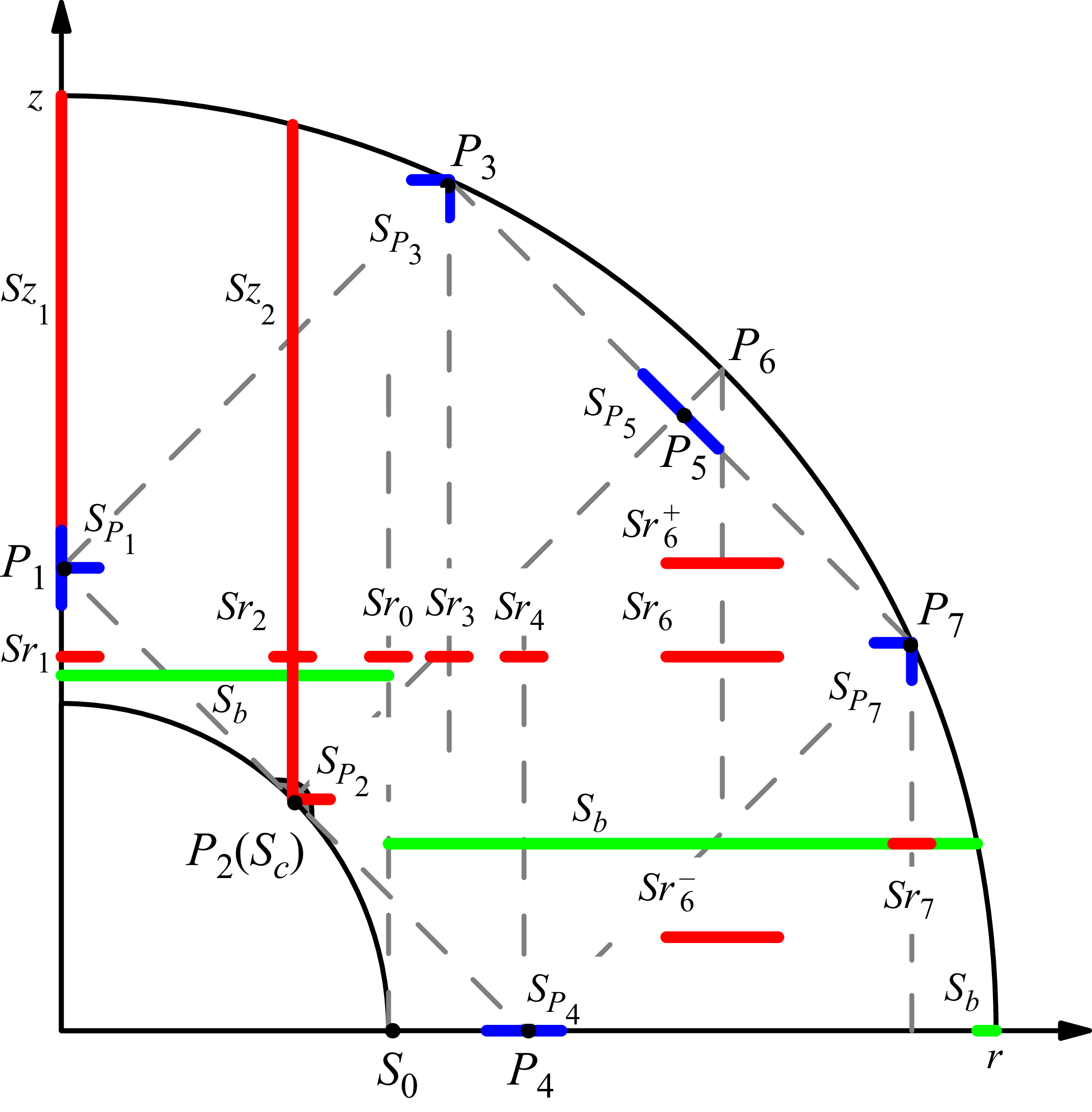
Schematic diagram of the positions of the slices used for comparing theoretical and NS (blue cuts). Green cuts are used to show the global bulk response. Red slices correspond to cases where only the NS is discussed.

4.1. Solution in the bulk generated from the boundary layers

In this section we consider the mean flow correction driven by oscillating boundary layers on the inner core. Such a correction was already examined by Sauret & Le Dizès (Reference Sauret and Le Dizès2013) in the absence of critical latitudes and inertial waves. They determined that the mean zonal flow within a spherical shell could be directly inferred from the analytical solutions derived for a full sphere. They showed that an azimuthal velocity of order $E^{0}$ was generated in the bulk, $v_{0\phi }=\mathcal{F}(\rho ;\omega )$ in their (4.27). Furthermore, they extended their analysis to cases where $0\lt \omega \lt 2$ , a condition in which inertial waves emerge and have a weak nonlinear effect on the fluid. Building upon this foundational work, Cébron et al. (Reference Cébron, Vidal, Schaeffer, Borderies and Sauret2021) expanded the theory to include non-homoeoidal spheroidal shells, accounting for variations in the amplitudes of libration forcing at different boundaries. They succinctly expressed the rotation velocity of the mean zonal flow in dimensionless form, presented as (5.5) in their publication.

Figure 5.

$(a)$ Mean azimuthal velocity $v_{0\phi }$ in the bulk as predicted by numerical computations (red solid line, $E = 10^{-10}$ ) and theoretical results (black dashed line, based on Sauret & Le Dizès Reference Sauret and Le Dizès2013 and Cébron et al. Reference Cébron, Vidal, Schaeffer, Borderies and Sauret2021). The light blue background highlights the interior region inside the tangent cylinder, located at $r = 0.35$ . $(b)$ Logarithm mean azimuthal velocity outside the tangent cylinder from numerical computations at different Ekman numbers. Inside the tangent cylinder, cuts are taken at $S_{b}$ and $z = 0.4$ . For the outer region, cuts are taken at $z = 0.2$ initially and then on the equator once the cut reaches the outer boundary; see figure 4. The directory containing the data and the Jupyter notebook used to compute the asymptotic theory and generate this figure can be accessed at https://multimediafluids.uam.elogim.com/S0022112025109841/JFM-Notebooks/files/Figure5/Figure5.ipynb.

In our study, we use (5.5) from Cébron et al. (2021), illustrating the theoretical predictions with a black dashed line in figure 5(a). Our numerical computations at $E=10^{-10}$ show excellent agreement with this theoretical prediction. This confirms that nonlinear effects within the Ekman boundary layer remain one of the important sources of mean zonal flow within the shell. Additionally, we identify two critical lines: $r=\eta /\sqrt {2}$ , which marks the critical latitude, and $r=\eta$ , denoting the cylinder tangent to the inner core boundary. Our numerical computations confirm that (5.5) from Cébron et al. (Reference Cébron, Vidal, Schaeffer, Borderies and Sauret2021) remains applicable even in the presence of inertial waves.

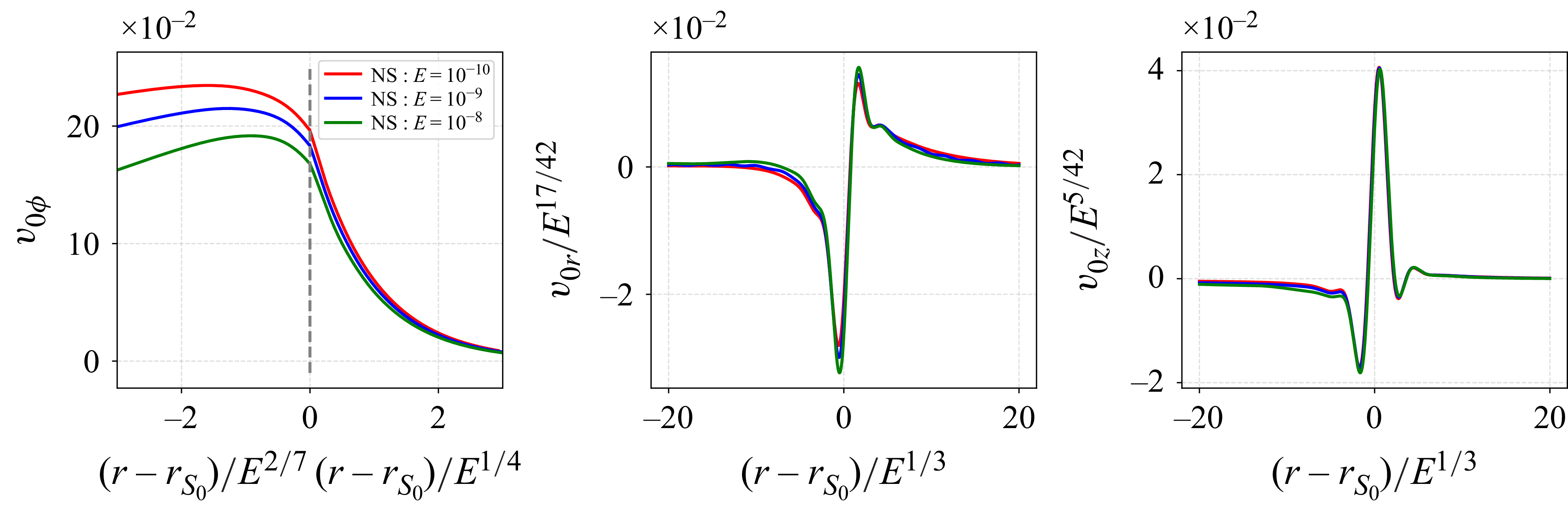
In the band issued from $S_0$ , which is tangent to the inner core, we expect Stewartson layers characterised by three distinct widths: $E^{2/7}$ for the internal layers, $E^{1/3}$ for the inner layer and $E^{1/4}$ for the external layers (Stewartson Reference Stewartson1966; Dormy & Soward Reference Dormy and Soward2007; Sauret & Le Dizès Reference Sauret and Le Dizès2013). In figure 6(a) the azimuthal velocity is plotted using the internal and external layer variables. The external scaling is perfectly recovered for this component. For the radial and axial velocity components, the scalings in $E^{17/42}$ and $E^{5/42}$ , which are predicted by the theory (Sauret & Le Dizès Reference Sauret and Le Dizès2013) in the inner layer, are compatible with the numerical results, as shown in figure 6(b,c).

Figure 6.

The length and amplitude scaling at $Sr_{0}$ are revealed from the NS by the velocity profiles of three Ekman numbers. The different scalings observed in the azimuthal velocity component $v_{0\phi }$ originate from the Stewartson layer.

It is important to note that previous theoretical frameworks generally assumed that the velocity outside the tangent cylinder remains zero when forcing is applied at the inner core boundary only. Contrary to this assumption, our numerical results shown in figure 5(b) reveal that this is not the case when inertial waves are present. We indeed observe a bulk azimuthal flow of order $E^{1/3}$ . Also visible are distinct peaks in the velocity profiles within the outer shell. These peaks correspond to specific regions where shear layers emitted from the critical latitude interact, either due to reflection on boundaries or through intersection within the volume. Although weak, these bands appear to exhibit the same scaling in $E^0$ as the mean flow generated by the boundary layer on the inner core. This observation provides important context for the subsequent research questions: What is the origin of these weak nonlinear zonal beams? How can we determine the corresponding amplitude and beam width? Addressing these questions constitutes one of the objectives of the present study. In the following sections we explain the origin of these weak nonlinear zonal beams and demonstrate the observed Ekman scaling.

4.2. Solution generated from the interaction along the beam

Equations (2.5) governing the mean flow correction read in cylindrical coordinates as

(4.1a) \begin{align} -2v_{0\phi }+\frac { \partial p_{0} }{ \partial r } & =-\mathcal{N}_{0r} + E\left (\Delta -\frac {1}{r^2}\right )v_{0r}, \end{align}

(4.1b) \begin{align} 2v_{0r} & =-\mathcal{N}_{0\phi } +E\left (\Delta -\frac {1}{r^2}\right )v_{0\phi }, \end{align}

(4.1c) \begin{align} \frac { \partial p_{0} }{ \partial z } & =-\mathcal{N}_{0z} +E\Delta v_{0z} , \end{align}

(4.1d) \begin{align} \frac {1}{r}\frac { \partial }{ \partial r } (rv_{0r})+\frac { \partial v_{0z} }{ \partial z } & =0 , \end{align}

where the Reynolds stress $\mathcal{N}_0=(\mathcal{N}_{0r}, \mathcal{N}_{0\phi }, \mathcal{N}_{0z})$ is given by

(4.2a) \begin{align} \mathcal{N}_{0r} & = v_{1r}\frac { \partial v_{1r}^{*} }{ \partial r } +v_{1z}\frac { \partial v_{1r}^{*} }{ \partial z } - \frac {v_{1\phi }v_{1\phi }^{*}}{r}+\mathrm{c}.\mathrm{c} , \end{align}

(4.2b) \begin{align} \mathcal{N}_{0\phi } & = v_{1r}\frac { \partial v_{1\phi }^{*} }{ \partial r } +v_{1z}\frac { \partial v_{1\phi }^{*} }{ \partial z } + \frac {v_{1r}v_{1\phi }^{*}}{r}+\mathrm{c}.\mathrm{c} , \end{align}

(4.2c) \begin{align} \mathcal{N}_{0z} & =v_{1r}\frac { \partial v_{1z}^{*} }{ \partial r } +v_{1z}\frac { \partial v_{1z}^{*} }{ \partial z } +\mathrm{c}.\mathrm{c} . \end{align}

The Reynolds stress expression can be simplified along the beam using the properties (3.10) and (3.11) that the harmonic solution satisfies. It gives, using (3.10) and (3.11),

(4.3a) \begin{align} &\mathcal{N}_{0r} \sim \frac {\partial }{\partial r}\left ( | v_{1r}|^2 - | v_{1z}| ^2\right ) - 4 \frac {| v_{1r} |^2 }{r} , \end{align}

(4.3b) \begin{align} & \mathcal{N}_{0\phi } \sim 2 \frac {\partial }{\partial z} \operatorname {Im}(v_{1r} v_{1z}^*) , \end{align}

(4.3c) \begin{align} & \mathcal{N}_{0z} \sim -\frac {\partial }{\partial z}\left ( | v_{1r}|^2 - | v_{1z}| ^2\right ) \! . \end{align}

If we neglect the viscous terms, a particular solution to (4.1) can be obtained as

(4.4a) \begin{align} &v_{0r} = - \frac {\partial }{\partial z} \operatorname {Im}(v_{1r} v_{1z}^*) , \end{align}

(4.4b) \begin{align} &v_{0\phi } = \frac {\partial }{\partial r}\left ( | v_{1r}|^2 - | v_{1z}| ^2\right ) - 2 \frac {| v_{1r} |^2 }{r} , \end{align}

(4.4c) \begin{align} &v_{0z} = \frac {1}{r}\frac {\partial }{\partial r} r \operatorname {Im}(v_{1r} v_{1z}^*) . \end{align}

As the harmonic velocity $\boldsymbol{v}_1$ varies with respect to a spatial variable that scales as $E^{1/3}$ for the main beam and as $E^{1/6}$ for the secondary beam, the viscous terms associated with the solution (4.4) remain small. This expression is therefore expected to be valid along the beam.

However, this solution is small, of order $E^{1/6}$ , when evaluated using (3.5), and of order $E^{1/2}$ , when evaluated using (3.7). It becomes large only when two beams intersect, that is, in the local regions $P_\beta$ . In the next subsections we provide the scaling and the expression of the solution in the three typical interaction regions.

4.2.1. Solution in the local regions $P_3$ , $P_4$ and $P_7$

Close to those points, the particular solution reduces, at leading order, to

(4.5) \begin{equation} \boldsymbol{v}_0 \sim \frac {1}{r}E^{-1/6} \boldsymbol{\tilde {v}}_0 , \end{equation}

with

(4.6) \begin{equation} \begin{pmatrix} \tilde {v}_{0r} \\[10pt] \tilde {v}_{0\phi } \\[10pt] \tilde {v}_{0z} \end{pmatrix}=\begin{pmatrix} \displaystyle {-\frac {1}{\sqrt {2}} \frac { \partial \widetilde {\mathcal{N}}_{P_\beta } }{ \partial \tilde {z}_\beta } } \\[8pt] \displaystyle { \frac { \partial \widetilde {\mathcal{M}}_{P_\beta } }{ \partial \tilde {r}_\beta } } \\[8pt] \displaystyle {\frac {1}{\sqrt {2}} \frac { \partial \widetilde {\mathcal{N}}_{P_\beta } }{ \partial \tilde {r}_\beta } } \end{pmatrix} , \end{equation}

where the functions $\widetilde {\mathcal{M}}_{P_{\beta }}$ and $\widetilde {\mathcal{N}}_{P_{\beta }}$ are given by

(4.7a) \begin{align} \widetilde {\mathcal{M}}_{P_{3}} = 2\mathrm{Re}\widetilde {\mathcal{Q}}_3,\qquad \widetilde {\mathcal{M}}_{P_{4}} = 2\mathrm{Re}\widetilde {\mathcal{Q}}_4 ,\qquad \widetilde {\mathcal{M}}_{P_{7}} = - 2\mathrm{Re}\widetilde {\mathcal{Q}}_7, \end{align}

(4.7b) \begin{align} \widetilde {\mathcal{N}}_{P_{3}} = -2\mathrm{Im}\widetilde {\mathcal{Q}}_3 ,\qquad \widetilde {\mathcal{N}}_{P_{4}} = -2\mathrm{Im}\widetilde {\mathcal{Q}}_4 ,\qquad \widetilde {\mathcal{N}}_{P_{7}} = -2\mathrm{Im}\widetilde {\mathcal{Q}}_7, \\[9pt] \nonumber \end{align}

with

(4.8) \begin{equation} \widetilde {\mathcal{Q}}_\beta (\tilde {r}_\beta ,\tilde {z}_\beta ) =\left(\tilde {B}_{\beta }^{\textit{Ni}}- \tilde {B}_{\beta }^{\textit{Sr}} \right)\left( \tilde {B}_{\beta }^{Nr*} - \tilde {B}_{\beta }^{Si*}\right)\! . \end{equation}

As it can be seen on these expressions, only four nonlinear contributions remain. They are all confined to the local interaction regions. This result aligns with the outcomes of our numerical computations and meets our expectations. This further supports the idea that the main sources of zonal flow are constrained to the $O(E^{1/3})$ regions where incident and reflected beams interact.

From (4.6), one can also obtain the normal and tangential velocity associated with this solution:

(4.9) \begin{equation} \tilde {v}_{0n}=-\frac {1}{\sqrt {2}} \frac { \partial \widetilde {\mathcal{N}}_{P_\beta } }{ \partial \tilde {x}_{t} } ,\qquad \tilde {v}_{0t}=\frac {1}{\sqrt {2}} \frac { \partial \widetilde {\mathcal{N}}_{P_\beta } }{ \partial \tilde {x}_{n} } . \end{equation}

Thanks to (3.17), one can see that expression (4.7) with (4.8) reduces at the boundary ( $\tilde {x}_n=0$ ) to $ \widetilde {\mathcal{N}}_{P_\beta } (\tilde {x}_n=0) = 0$ . This implies that the normal velocity vanishes at the boundary. The non-penetration condition is then automatically satisfied. This has an important consequence. It means that the particular solution (4.6) is the leading-order solution in each local region around $P_\beta$ . It is this expression that will be compared to the NS close to each $P_\beta$ . Since the functions $ \widetilde {\mathcal{M}}_{P_\beta }$ and $\widetilde {\mathcal{N}}_{P_\beta }$ are both localised, all the velocity components are also localised near $P_\beta$ at this order.

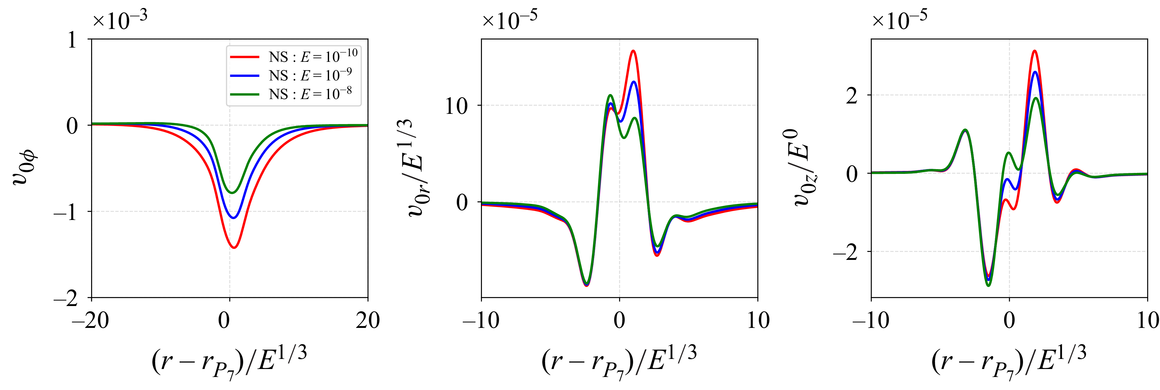
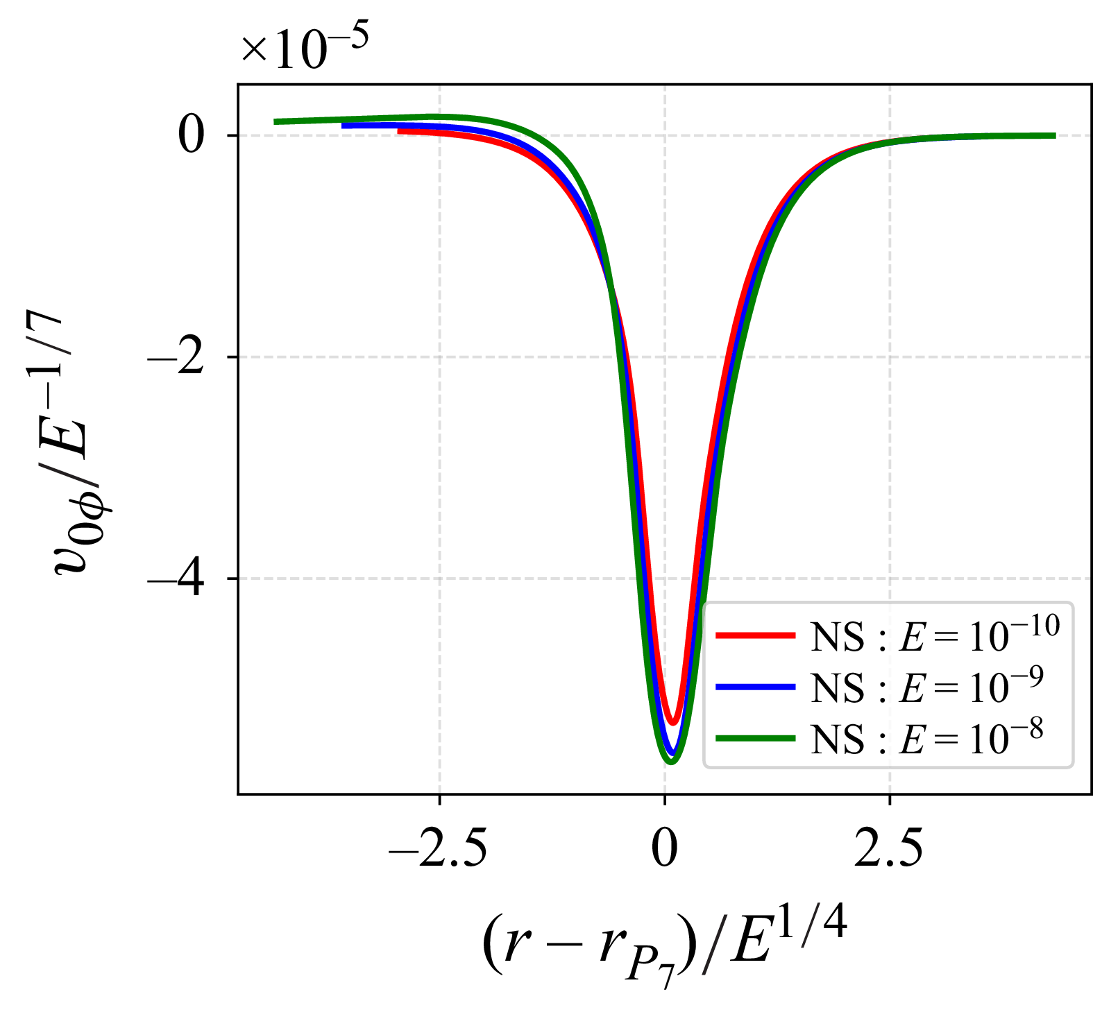
Figure 7 compares the profiles of three asymptotic velocity components with NS for three different Ekman numbers near $P_7$ . The comparison is performed on the vertical and horizontal slices $S_{P_7}$ , as depicted in figure 4. As expected, the asymptotic theoretical results increasingly align with the numerical data as the Ekman number decreases. However, discrepancies are observed in the radial velocity, $v_{0r}$ , and the axial velocity, $v_{0z}$ , near the boundary. These discrepancies arise because the numerical boundary condition employs a no-slip condition, causing the NS to approach zero at the boundary, while only the non-penetration condition is satisfied by the AS. As demonstrated in Le Dizès (Reference Le Dizès2020), another approximation can be constructed in a viscous boundary layer of $O(E^{1/2})$ width to capture this behaviour.

In addition, the azimuthal velocity along the $z$ axis, parallel to the rotation axis, tends to zero in the asymptotic theory as one moves away from the local interaction point. However, numerical results display a small amplitude zonal flow in the bulk (see the bottom left panel of figure 7). This is also evident in figure 1, where several weak bands are visible throughout the bulk. The scaling of these bands will be discussed in the next section, using the results given in Appendix C.

Figure 7.

Three velocity component profiles of the $AS$ and the NS for three different Ekman numbers at local region $P_7$ with two direction cuts ( $S_{P_7}$ in figure 4). The directory containing the data and the Jupyter notebook used to compute the asymptotic theory and generate this figure can be accessed at https://multimediafluids.uam.elogim.com/S0022112025109841/JFM-Notebooks/files/Figure7/Figure7.ipynb.

Figure 8.

Same caption as figure 7 but at local region $P_3$ (cuts at $S_{P_3}$ ). The directory containing the data and the Jupyter notebook used to compute the asymptotic theory and generate this figure can be accessed at https://multimediafluids.uam.elogim.com/S0022112025109841/JFM-Notebooks/files/Figure8/Figure8.ipynb.

Figure 9.

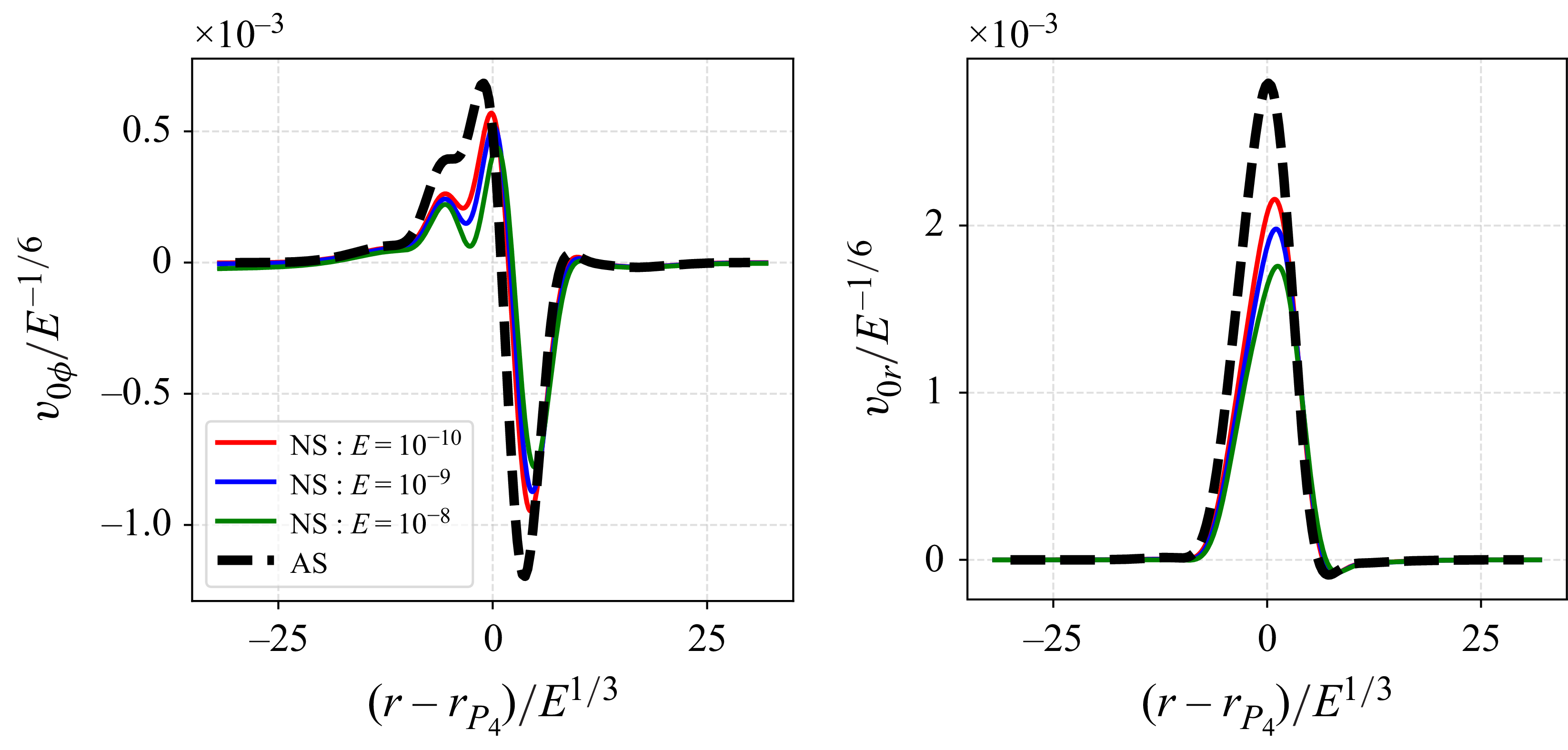
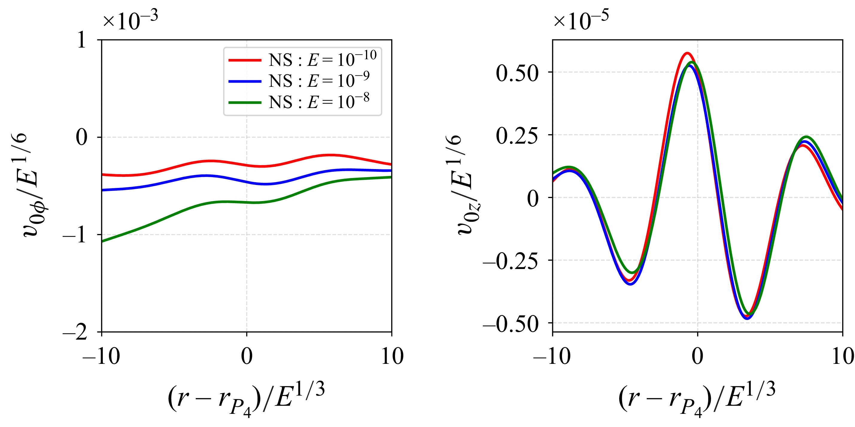
Comparison of AS and NS of two velocity components ( $v_{0z}=0$ ) at local region $P_4$ (cuts position at $S_{P_4}$ ). The directory containing the data and the Jupyter notebook used to compute the asymptotic theory and generate this figure can be accessed at https://multimediafluids.uam.elogim.com/S0022112025109841/JFM-Notebooks/files/Figure9/Figure9.ipynb.

Comparisons between two similar interaction regions, $P_3$ and $P_4$ , and the numerical results are presented in figures 8 and 9, respectively. The observations from figure 7 regarding differences in the boundary layer and the azimuthal velocity in the bulk are also applicable here. Notably, near $P_4$ , located on the equatorial plane, the axial velocity $v_{0z}$ remains zero by symmetry. Additionally, improvements in the comparison with decreasing Ekman numbers are observed, consistent with the findings at other local positions.

At the three specific locations $P_7$ , $P_3$ and $P_4$ the asymptotic analysis yielded consistent scaling behaviours: the interaction region scales as $E^{1/3}$ and the amplitude scales as $E^{-1/6}$ for all three velocity components. Note however that the rescaled velocity remains small, of order $10^{-3}$ , at each of these points. This explains why these regions are not more visible on the contour map shown in figure 1.

4.2.2. Solution in the local regions $P_5$ and $P_6$

The secondary weak beams encounter the main critical beam in the bulk at $P_5$ . This case is interesting because the scalings of the two beams differ.

The mean flow correction is weaker and given by

(4.10) \begin{equation} \boldsymbol{v}_{0}\sim \frac {1}{r}E^{0}\boldsymbol{\breve {v}}_{0} , \end{equation}

with

(4.11) \begin{equation} \begin{pmatrix} \breve {v}_{0r} \\[10pt] \breve {v}_{0\phi } \\[10pt] \breve {v}_{0z} \end{pmatrix} =\begin{pmatrix} \displaystyle {-\frac {1}{\sqrt {2}} \frac { \partial \breve {\mathcal{N}}_{P_5} }{ \partial \tilde {z}_5 } } \\[8pt] \displaystyle { \frac { \partial \breve {\mathcal{M}}_{P_5} }{ \partial \tilde {r}_5 } } \\[8pt] \displaystyle {\frac {1}{\sqrt {2}} \frac { \partial \breve {\mathcal{N}}_{P_5} }{ \partial \tilde {r}_5 } } \end{pmatrix}, \end{equation}

where

(4.12) \begin{align} \breve {\mathcal{M}}_{P_5} & = 2\operatorname {Re} \left ( \left( \breve {B}^{N}- \breve {B}^{S}\right) \left( \tilde {B}_{5}^{N*} -\tilde {B}_{5}^{S*}\right) \right )\! , \end{align}

(4.13) \begin{align} \breve {\mathcal{N}}_{P_5} & = -2 \operatorname {Im}\left ( \left( \breve {B}^{N}- \breve {B}^{S}\right) \left( \tilde {B}_{5}^{N*} -\tilde {B}_{5}^{S*}\right) \right )\!. \\[12pt] \nonumber\end{align}

These expressions are similar to that obtained near point $P_4$ , where the $Nr$ and $Si$ beams at $P_4$ are now the strong $S$ and $N$ beams propagating between $P_3$ and $P_7$ , while $Ni$ and $Sr$ beams at $P_4$ are the weak $S$ and $N$ beams propagating between $P_2$ and $P_6$ (see figure 2 b). Note that because $\breve {B}^S$ and $\breve {B}^N$ are functions of the slow variable $\breve {x}_\perp = E^{1/6} (\tilde {z}_5-\tilde {r}_5)/\sqrt {2}$ , the spatial derivatives in (4.11) should be applied to $\tilde {B}_{5}^{S}$ and $\tilde {B}_{5}^{N}$ only.

Figure 10.

Comparison of the AS and NS of velocity profiles at local region $P_{5}$ (cuts at $S_{P_5}$ ). The directory containing the data and the Jupyter notebook used to compute the asymptotic theory and generate this figure can be accessed at https://multimediafluids.uam.elogim.com/S0022112025109841/JFM-Notebooks/files/Figure10/Figure10.ipynb.

In figure 10 we compare the AS from (4.11) with numerical results for three different Ekman numbers. The secondary weak beam, characterised by its larger width scaling in $E^{1/6}$ , is analysed by taking profile cuts parallel to the critical beam from $P_3$ to $P_7$ (see figure 4, $S_{P_5}$ ). Due to the anti-symmetry of the weak beam, the cuts in the perpendicular direction (that is on the $z = r$ line) are zero.

The width of the local region scales as $E^{1/6}$ , while the other direction scales as $E^{1/3}$ . The amplitude scaling is $E^{0}$ , which is significantly weaker than in other local interaction regions. Despite the two beams having different scaling factors, the asymptotic method demonstrates overall accuracy. The asymptotic theory matches the NS well, exhibiting convergence as the Ekman number decreases.

However, some perturbations are observed on the right-hand side of figure 10, specifically in the $v_{0\phi }$ component. These perturbations arise because the cut profiles are influenced by the weak band issued from the point $P_6$ , as shown in figure 5(b).

In the local region $P_6$ , a particular solution of the same form as (4.11) can be obtained. However, as we will see in § 5 and Appendix C, this particular solution is modified by an additional homogeneous solution, which describes the mean flow correction associated with the vertical band originating from $P_6$ . Therefore, it cannot be directly compared to numerical results.

4.2.3. Solution in the local region $P_1$

For the point on the rotation axis, we must use the expressions (3.23) for the harmonic solution. We obtain the following expression for the mean flow:

(4.14) \begin{equation} \boldsymbol{v}_0=E^{-1/2} \boldsymbol{\hat {v}}_{0} \end{equation}

with

(4.15a) \begin{align} \hat {v}_{0r} & = -\frac {1}{\sqrt {2}}\frac {\partial }{\partial \tilde {z}_1} \left \{\operatorname {Re}\left [ \left(Q^{N}_{1}+ Q^{S}_{1}\right)\left(-Q^{N*}_{0}+Q^{S*}_{0}\right) \right ]\right \}, \end{align}

(4.15b) \begin{align} \hat {v}_{0\phi } & = \frac {1}{2}\frac {\partial }{\partial \tilde {r}_1} \left \{\left |Q^{N}_{1}+Q^{S}_{1}\right |^2 - \left |-Q^{N}_0 + Q^S_0\right |^2 \right \} - \frac {\left |Q^{N}_{1}+Q^{S}_{1}\right |^2 }{\tilde {r}_1}, \end{align}

(4.15c) \begin{align} \hat {v}_{0z} & = \frac {1}{\sqrt {2}}\left (\frac {\partial }{\partial \tilde {r}_1}+ \frac {1}{\tilde {r}_1} \right )\left \{\operatorname {Re}\left [ \left(Q^{N}_{1}+ Q^{S}_{1}\right)\left(-Q^{N*}_{0}+Q^{S*}_{0}\right) \right ]\right \} . \\[12pt] \nonumber \end{align}

In figure 11 we compare the AS from (4.15) with numerical results for three different Ekman numbers. The profiles analysed are taken at $S_{P_1}$ and include one profile in the direction perpendicular to the rotation axis and another along the rotation axis (see figure 4). Due to the axisymmetry of the system, only the axial velocity component is considered along the rotation axis, as the two other components, $v_{0r}$ and $v_{0\phi }$ , are identically zero.

The width of the local region scales with $E^{1/3}$ , while the amplitude scales with $E^{-1/2}$ . Although the overall agreement between the AS and the numerical results is strong, particularly for the azimuthal component, a noticeable deviation is observed in the smaller $v_{0r}$ component near the axis. This discrepancy was already observed in the linear harmonic solution in He et al. (Reference He, Favier, Rieutord and Le Dizès2022). We suspect that it could come from higher-order corrections that could become non-negligible owing to the smallness of the solution at this leading order.

Figure 11.

Comparison of the AS and NS of velocity profiles at local region $P_1$ (cuts position at $S_{P_1}$ ). The directory containing the data and the Jupyter notebook used to compute the asymptotic theory and generate this figure can be accessed at https://multimediafluids.uam.elogim.com/S0022112025109841/JFM-Notebooks/files/Figure11/Figure11.ipynb.