1 Introduction
A powder snow avalanche is a flowing, fluidised suspension of fine snow, fed by new snow that is ejected from the underlying surface due to large pressure gradients near the head of the avalanche, sometimes referred to as an eruption current (Sovilla, Burlando & Bartelt Reference Sovilla, Burlando and Bartelt2006; Louge, Carroll & Turnbull Reference Louge, Carroll and Turnbull2011). This is in contrast to more commonly studied examples of gravity currents, which are formed by the release of a fixed mass of the particulate substance that then moves under the action of gravity without further replenishment (Simpson Reference Simpson1997). The presence of a source of new particulate material close to the head of the flow fundamentally changes its dynamics, and may allow an eruption current to propagate further than a simple gravity current. In Carroll, Turnbull & Louge (Reference Carroll, Turnbull and Louge2012), the authors consider a sequence of two-dimensional models of powder snow avalanches, in each of which the snow that erupts into the current is modelled as either a point source in an inviscid, irrotational flow or as a numerical approximation of a point source within a large eddy simulation of the variable density Navier–Stokes equations. In this paper we revisit the first of these models, in which the fluidised snow is modelled as inviscid and incompressible, and is assumed to flow irrotationally from a moving point source surrounded by stationary, ambient, immiscible, inviscid fluid of lower density. When the fluid densities are equal, in a frame of reference moving at velocity
 $U>0$
with the point source of strength
 $q$
at its origin, the flow is given in polar coordinates
 $(r,\unicode[STIX]{x1D703})$
by the velocity potential
 $$\begin{eqnarray}\unicode[STIX]{x1D719}=-Ur\cos \unicode[STIX]{x1D703}+\frac{q}{\unicode[STIX]{x03C0}}\log r,\end{eqnarray}$$
in
 $0\leqslant \unicode[STIX]{x1D703}\leqslant \unicode[STIX]{x03C0}$
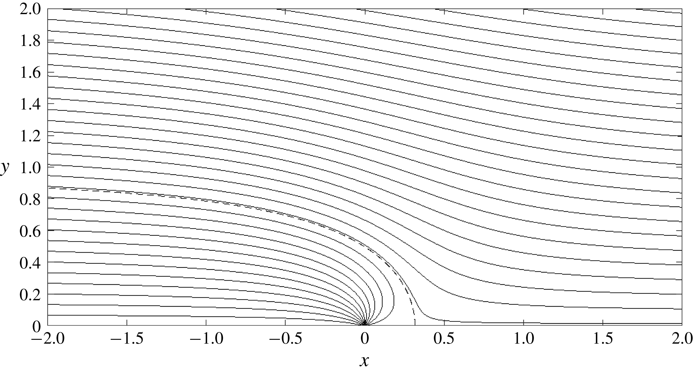
. Some typical streamlines are shown in figure 1, and are equivalent to those around a Rankine body given by
 $$\begin{eqnarray}x=y\cot \left(\frac{\unicode[STIX]{x03C0}Uy}{q}\right),\end{eqnarray}$$
in Cartesian coordinates
 $(x,y)$
(see, for example, Batchelor Reference Batchelor1967). In terms of the problem that we are interested in, equation (1.2) gives the dividing streamline between fluid 2 and fluid 1, which originates at the source, when the fluids have equal density.
A unit source at
 $x=y=0$
in a unit flow from right to left when the two fluids have equal density, given by the velocity potential
 $\unicode[STIX]{x1D719}=-x+(1/\unicode[STIX]{x03C0})\log r$
and corresponding streamfunction
 $\unicode[STIX]{x1D713}=-y+\unicode[STIX]{x1D703}/\unicode[STIX]{x03C0}$
. The streamline that meets the stagnation point on the boundary at
 $x=1/\unicode[STIX]{x03C0}$
,
 $y=0$
and which represents the position of the free surface,
 $x=y\cot \unicode[STIX]{x03C0}y$
(equivalently
 $y=\unicode[STIX]{x1D703}/\unicode[STIX]{x03C0}$
), is shown as a broken line.

We find that the flow in this nonlinear, two fluid, free boundary problem is more complex than is suggested by the results presented in Carroll et al. (Reference Carroll, Turnbull and Louge2012). Unless the fluids have equal density, no steady solution exists because of the likely non-existence of a steady local solution in the neighbourhood of the contact point (at
 $y=0$
). We therefore analyse the dynamics of the flow by studying an initial value problem in which the initial velocity field is given by (1.1) and the fluids are initially separated by the free surface given by (1.2). Later in the paper, we also consider the flow when the initial position of the free surface is a nearby streamline of this flow, for reasons that will be become clear as we progress. The difference in density between the fluids drives the subsequent development of the flow and motion of the free surface. Although it may seem more natural to study what happens when a source of slightly denser fluid is injected ab initio, we are interested in how the dynamics of this flow is related to fully developed powder snow avalanches, for which the initial conditions that we have chosen are more relevant.
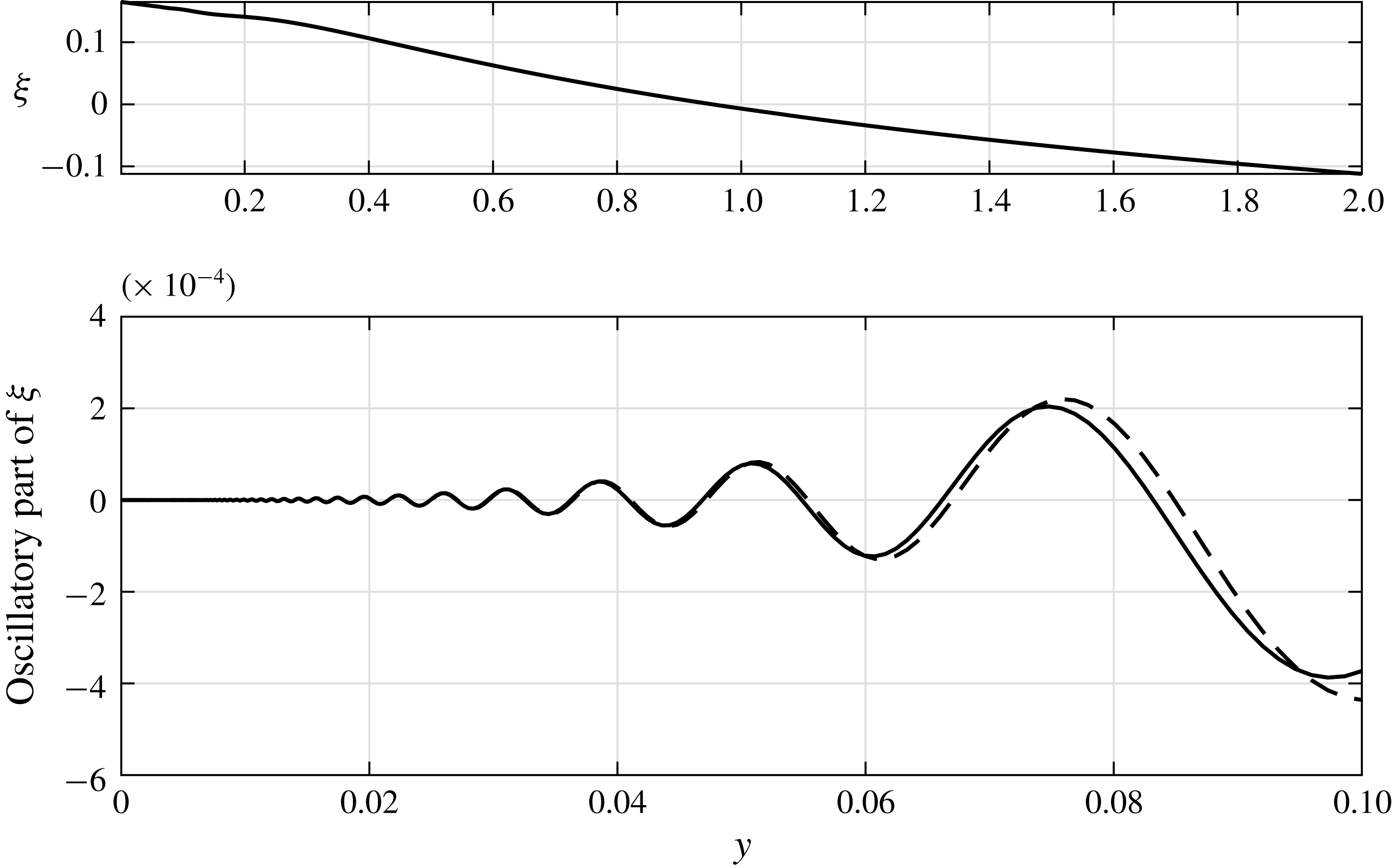
In § 2, we set up the governing equations for this initial/boundary value problem. We study the problem in the limit of small density difference in § 3, and show that the head of the layer of fluid 1 (to the right of the source) swells and the contact point moves rapidly forwards close to the initial stagnation point. In addition, a disturbance propagates downstream at the speed of the source, which is a stationary initial transient in a frame of reference fixed in the boundary. In § 4 we examine the initial behaviour of the flow, in particular near the stagnation point where the interface meets the solid surface. We find that this is locally a dam break, which means that we need to use the method of matched asymptotic expansions, in the same manner as King & Needham (Reference King and Needham1994) and Uddin & Needham (Reference Uddin and Needham2015), to determine the initial dynamics of the flow. Close to the contact point, we find that the free boundary takes a spatially oscillatory form, with a wavelength that tends to zero as
 $y\rightarrow 0$
. We also find that in this region the Boussinesq approximation,
 $\bar{\unicode[STIX]{x1D70C}}\ll 1$
and
 $\bar{Ri}=O(1)$
, which it is natural to consider in the outer flow (although it is not relevant to avalanches), is a singular limit. In § 5, we discuss numerical solutions of the fully nonlinear free boundary problem, computed using an adaptive vortex blob method, which allows us to study the nonlinear development of the initial disturbance. We find that nonlinear effects (Kelvin–Helmholtz instability) can cause the disturbance that propagates along the layer to overturn. For non-zero Richardson number, we regularise the flow close to the contact point by using an initial free surface with a thin layer of fluid 1 that extends to infinity ahead of the source. In this case, overturning can also occur at the head of the layer for sufficiently large Richardson number.
2 Governing equations
Using the source velocity,
 $U$
, and the flux from the source,
 $q$
, we can form length and time scales,
 $L\equiv q/U$
and
 $T\equiv q/U^{2}$
. We use these to non-dimensionalise the governing equations in a frame of reference moving with the source. The initial/boundary value problem that we will study, defined by (2.2)–(2.8) below, contains just two dimensionless parameters constructed from these quantities: the dimensionless density difference and the Richardson number,
 $$\begin{eqnarray}\bar{\unicode[STIX]{x1D70C}}=\frac{\unicode[STIX]{x1D70C}_{1}-\unicode[STIX]{x1D70C}_{2}}{\unicode[STIX]{x1D70C}_{2}}\geqslant 0,\quad Ri=\frac{(\unicode[STIX]{x1D70C}_{1}-\unicode[STIX]{x1D70C}_{2})gq}{\unicode[STIX]{x1D70C}_{2}U^{3}}\equiv \bar{\unicode[STIX]{x1D70C}}\frac{gL}{U^{2}}\equiv \bar{\unicode[STIX]{x1D70C}}\bar{Ri}\geqslant 0.\end{eqnarray}$$
In a powder snow avalanche, the density of the fluidised snow is typically between two and ten times greater than that of the surrounding air, the height of the avalanche is between 20 and 50 m, and typical propagation speeds lie between
 $15$
and
 $50~\text{m}~\text{s}^{-1}$
. This leads to the approximate parameter ranges
 $1\leqslant \bar{\unicode[STIX]{x1D70C}}\leqslant 10$
,
 $0.1\leqslant Ri\leqslant 20$
and
 $0.1\leqslant \bar{Ri}\leqslant 2$
. The Richardson number quantifies the importance of the effective gravitational force on the flow compared to that of the relative acceleration of the two fluids (the Bernoulli effect).
The two-dimensional domain of solution is
 $y\geqslant 0$
,
 $-\infty <x<\infty$
in Cartesian coordinates. We denote by
 ${\mathcal{D}}_{i}(t)$
the region occupied by the fluid of density
 $\unicode[STIX]{x1D70C}_{i}$
with velocity potential
 $\unicode[STIX]{x1D719}_{i}(\boldsymbol{x},t)$
, where
 $t\geqslant 0$
is time,
 $\boldsymbol{x}=(x,y)$
and
 $i=1$
or 2. The boundary
 $\unicode[STIX]{x2202}{\mathcal{D}}(t)$
between these two regions is given by
 $\boldsymbol{x}=\boldsymbol{X}(s,t)\equiv (X(s,t),Y(s,t))$
, where
 $s$
is the arclength along the free surface, with
 $s=0$
at the point
 $x=X_{c}(t)$
where
 $\unicode[STIX]{x2202}{\mathcal{D}}$
meets the boundary,
 $y=0$
. The irrotational flow of the two incompressible, inviscid fluids is governed by
 $$\begin{eqnarray}\unicode[STIX]{x1D6FB}^{2}\unicode[STIX]{x1D719}_{i}=0\quad \text{in}~{\mathcal{D}}_{i},\end{eqnarray}$$
with the kinematic boundary condition
 $$\begin{eqnarray}\boldsymbol{n}\boldsymbol{\cdot }\frac{\unicode[STIX]{x2202}\boldsymbol{X}}{\unicode[STIX]{x2202}t}=\boldsymbol{n}\boldsymbol{\cdot }\unicode[STIX]{x1D735}\unicode[STIX]{x1D719}_{1}=\boldsymbol{n}\boldsymbol{\cdot }\unicode[STIX]{x1D735}\unicode[STIX]{x1D719}_{2}\quad \text{at}~\boldsymbol{x}=\boldsymbol{X}(s,t),\end{eqnarray}$$
where
 $\boldsymbol{n}$
is the outward unit normal to
 ${\mathcal{D}}_{1}$
, along with the dynamic boundary condition,
 $$\begin{eqnarray}(1+\bar{\unicode[STIX]{x1D70C}})\left(\frac{\unicode[STIX]{x2202}\unicode[STIX]{x1D719}_{1}}{\unicode[STIX]{x2202}t}+\frac{1}{2}|\unicode[STIX]{x1D735}\unicode[STIX]{x1D719}_{1}|^{2}\right)-\left(\frac{\unicode[STIX]{x2202}\unicode[STIX]{x1D719}_{2}}{\unicode[STIX]{x2202}t}+\frac{1}{2}|\unicode[STIX]{x1D735}\unicode[STIX]{x1D719}_{2}|^{2}\right)=-RiY\quad \text{at}~\boldsymbol{x}=\boldsymbol{X}(s,t).\end{eqnarray}$$
Note that we have set the Bernoulli constant to zero, but that this is somewhat arbitrary, since the interface does not extend to infinity upstream. The no penetration condition at the solid boundary is
 $$\begin{eqnarray}\frac{\unicode[STIX]{x2202}\unicode[STIX]{x1D719}_{1}}{\unicode[STIX]{x2202}y}=\frac{\unicode[STIX]{x2202}\unicode[STIX]{x1D719}_{2}}{\unicode[STIX]{x2202}y}=0\quad \text{at}~y=0.\end{eqnarray}$$
Although (2.3) shows that the normal derivatives of the potentials, and hence normal velocities, are continuous at the boundary, the potentials and their tangential derivatives (the tangential velocities) need not be continuous in this inviscid model. We must also include the source of fluid 1 at the origin,
 $$\begin{eqnarray}\unicode[STIX]{x1D719}_{1}\sim \frac{1}{\unicode[STIX]{x03C0}}\log r\quad \text{as}~r\equiv \sqrt{x^{2}+y^{2}}\rightarrow 0,\end{eqnarray}$$
and the upstream flow of fluid 2 in this frame of reference,
 $$\begin{eqnarray}\unicode[STIX]{x1D719}_{2}\sim -x\quad \text{as}~x\rightarrow \infty .\end{eqnarray}$$
Finally, we take the initial position of the free surface to be the Rankine surface for the flow with equal densities, given by (1.2), so that
 $$\begin{eqnarray}X=Y\cot \unicode[STIX]{x03C0}Y\quad \text{when}~t=0,\end{eqnarray}$$
and hence when
 $t=0$
,
 ${\mathcal{D}}_{1}$
is the region
 $0\leqslant y\leqslant Y$
for
 $x\leqslant 1/\unicode[STIX]{x03C0}$
, with
 ${\mathcal{D}}_{2}$
the remainder of the upper half-plane. Although this is not an entirely obvious choice of initial condition – the fluids do not have equal density, so this is not an equilibrium solution, and the larger the density difference, the more rapidly the interface between the fluids evolves away from the initial condition – it has several advantages over other, more arbitrary choices, including: (i) it consists of a semi-infinite layer of the denser fluid, a geometry that we must preserve in order to be relevant to powder snow avalanches, (ii) it is close to an equilibrium solution when the density difference is small, so we can use a weakly nonlinear analysis to obtain insight into the development of the flow, (iii) it is easily modified to include a thin layer of the denser fluid stretching to infinity ahead of the source (see § 5), (iv) it is well defined and easy to implement both analytically and numerically. Although we have not tried to use any other initial conditions, it seems reasonable that the results below capture, at least qualitatively, the nature of the flow that would develop from similar initial conditions. Note also that in §§ 3 and 4, we will usually assume (correctly) that the free surface can be written as a single-valued function in polar coordinates,
 $r=R(\unicode[STIX]{x1D703},t)$
, with corresponding initial condition
 $R(\unicode[STIX]{x1D703},0)=\unicode[STIX]{x1D703}/\unicode[STIX]{x03C0}\sin \unicode[STIX]{x1D703}$
, or as
 $y=Y(x,t)$
with
 $x=Y(x,0)\cot \unicode[STIX]{x03C0}Y(x,0)$
or as
 $x=X(y,t)$
, with
 $X(y,0)=y\cot \unicode[STIX]{x03C0}y$
, in Cartesian coordinates. In § 5, we will use a Lagrangian representation of the free surface, which can accommodate overturning, as part of our numerical solution method for the full initial/boundary value problem.
Although
 $\unicode[STIX]{x1D719}_{1}=\unicode[STIX]{x1D719}_{2}$
when
 $t=0$
, as the inviscid, irrotational flow develops, a discontinuity in the tangential derivatives of these potentials, and hence a tangential velocity discontinuity, develops at the free surface. Locally, this will resemble planar, inviscid, two fluid flow with a velocity discontinuity. Flows like this are known to be subject to Kelvin–Helmholtz instability (for example, Batchelor Reference Batchelor1967), which usually leads to the development of a curvature singularity in finite time (for example, Moore Reference Moore1978; Cowley, Baker & Tanveer Reference Cowley, Baker and Tanveer1999), which can be regularised by adding some extra physics to the model, usually surface tension, although this is not the physics that we will add in this paper. We will address this issue in detail in § 5.
3 Asymptotic solution for flows with small density difference (
 $\bar{\unicode[STIX]{x1D70C}}\ll 1$
,
$\bar{Ri}=O(1)$
– the Boussinesq approximation)


Although we have seen that
 $\bar{\unicode[STIX]{x1D70C}}$
is not small for powder snow avalanches, it is natural to consider the Boussinesq limit,
 $\bar{\unicode[STIX]{x1D70C}}\ll 1$
with
 $\bar{Ri}=O(1)$
, as a way to gain insight into the dynamics of the flow and provide a test for numerical solutions of the full problem. As we shall see, in this limit the head of the layer swells and a depression propagates back along the layer at unit speed. We will see in § 5 that this is also how the flow behaves when
 $\bar{\unicode[STIX]{x1D70C}}$
is not small. We will also discover that there is a singularity in the shape of the free surface close to the contact point (a dam break), which persists when
 $\bar{\unicode[STIX]{x1D70C}}$
is not small. The mathematical details of our analysis are given in appendix A.
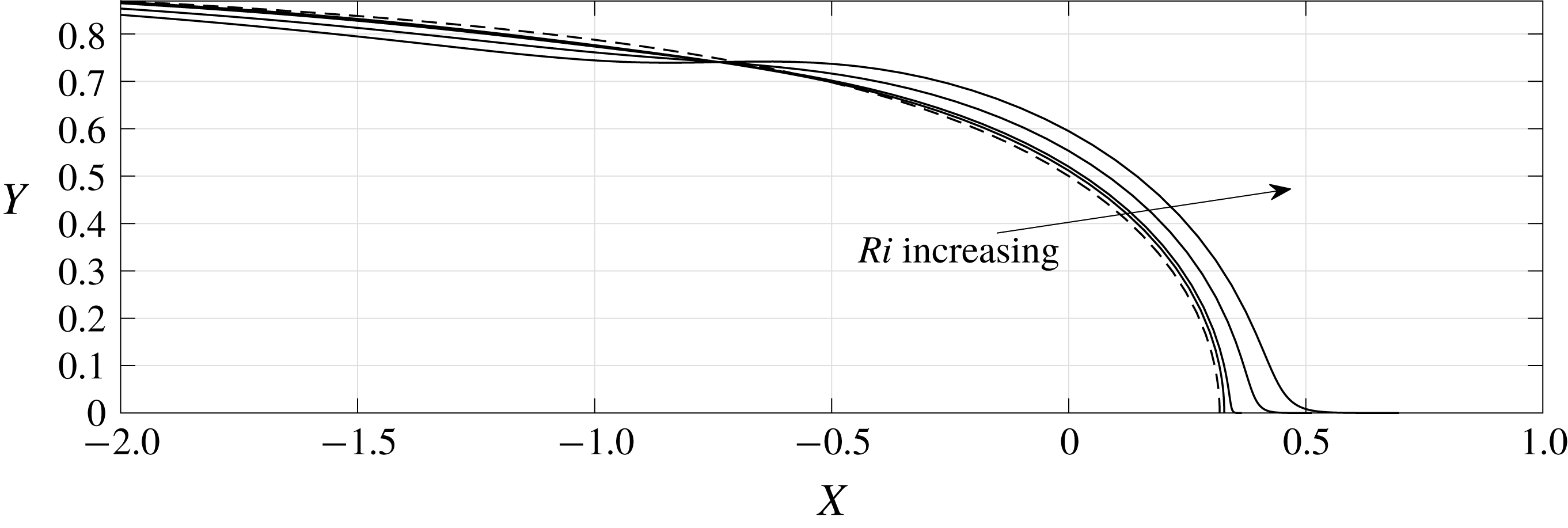
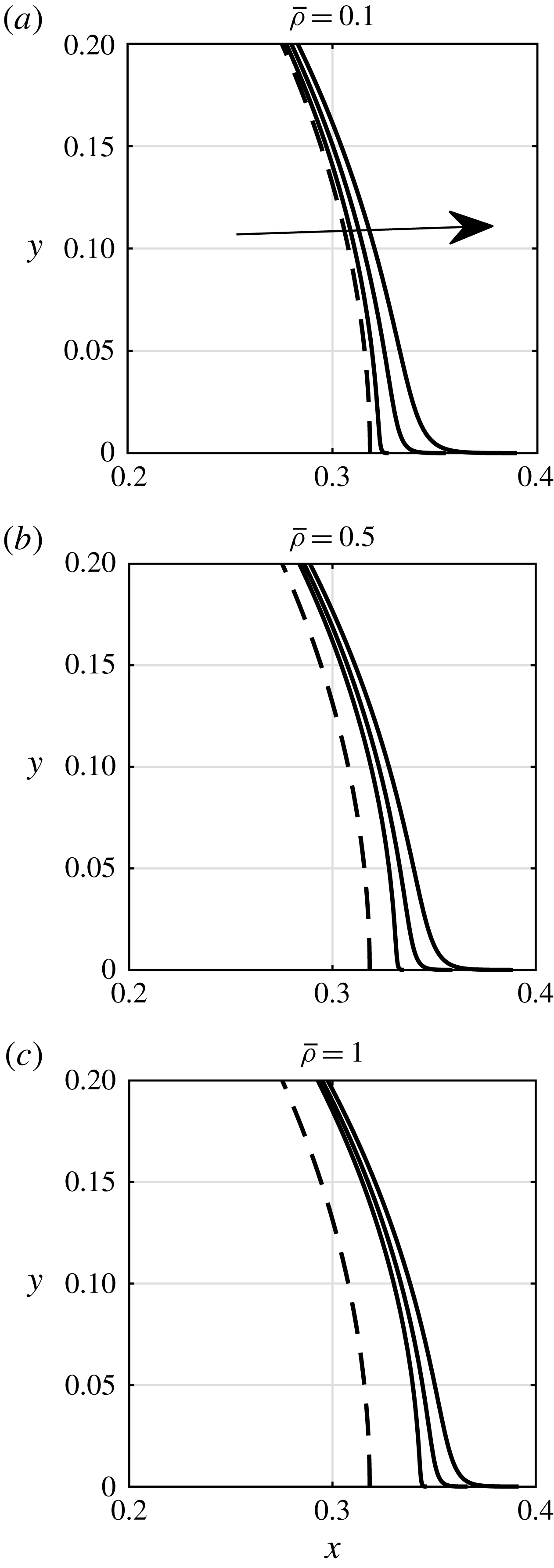
The position of the free surface for
 $\bar{\unicode[STIX]{x1D70C}}=0.1$
and
 $\bar{Ri}=0$
, 1, 5 and 10 when
 $t=1$
, calculated from the asymptotic solution for
 $\bar{\unicode[STIX]{x1D70C}}\ll 1$
. The initial position of the free surface is shown as a broken line.

Figure 2 shows the position of the free boundary when
 $t=1$
for
 $\bar{\unicode[STIX]{x1D70C}}=0.1$
and various values of
 $\bar{Ri}$
, calculated using the asymptotic solution for
 $\bar{\unicode[STIX]{x1D70C}}\ll 1$
. This somewhat large value of
 $\bar{\unicode[STIX]{x1D70C}}$
has been chosen to allow the position of the interface to be seen more clearly. In each case, the layer swells at the head, with the size of the swelling increasing with
 $\bar{Ri}$
and
 $\bar{\unicode[STIX]{x1D70C}}$
, whilst a depression propagates back down the layer at unit speed. Note that when
 $\bar{Ri}=0$
(the zero gravity case), the free surface remains perpendicular to the boundary,
 $y=0$
, and the speed of the contact point asymptotes to zero as
 $t\rightarrow \infty$
. When
 $\bar{Ri}>0$
, a thin layer of fluid 1 protrudes into fluid 2 close to the boundary, with the shape of the free surface very different to that in the zero gravity case. This is because there is a logarithmic singularity in the position of the free surface as
 $y\rightarrow 0$
, which we have not dealt with explicitly in our evaluation of the integral in (A 18), and is therefore removed by rounding error when
 $y=0$
. The behaviour close to the boundary when
 $Ri=O(1)$
and
 $t\ll 1$
is the subject of § 4, and includes the limit
 $\bar{\unicode[STIX]{x1D70C}}\ll 1$
, which we have studied in this section, as a subcase. In order to see why there is a singularity, consider the dynamic boundary condition, equation (2.4). Initially, the free surface is perpendicular to the boundary,
 $y=0$
, so we can differentiate (2.4) with respect to
 $y$
, and use the no penetration condition, equation (2.5), to show that the left hand side is then zero. The right-hand side is, however, non-zero, and it is this incompatibility in the boundary conditions that leads to a singularity in the outer flow when
 $t\ll 1$
. This incompatibility is reconciled in a small inner region close to the point of contact of the free surface with the boundary which, crucially, moves with an algebraically small velocity and a logarithmically large acceleration as
 $t\rightarrow 0$
. In § 5 we determine an equation for the motion of the contact point, equation (5.7), that holds for all
 $t>0$
.
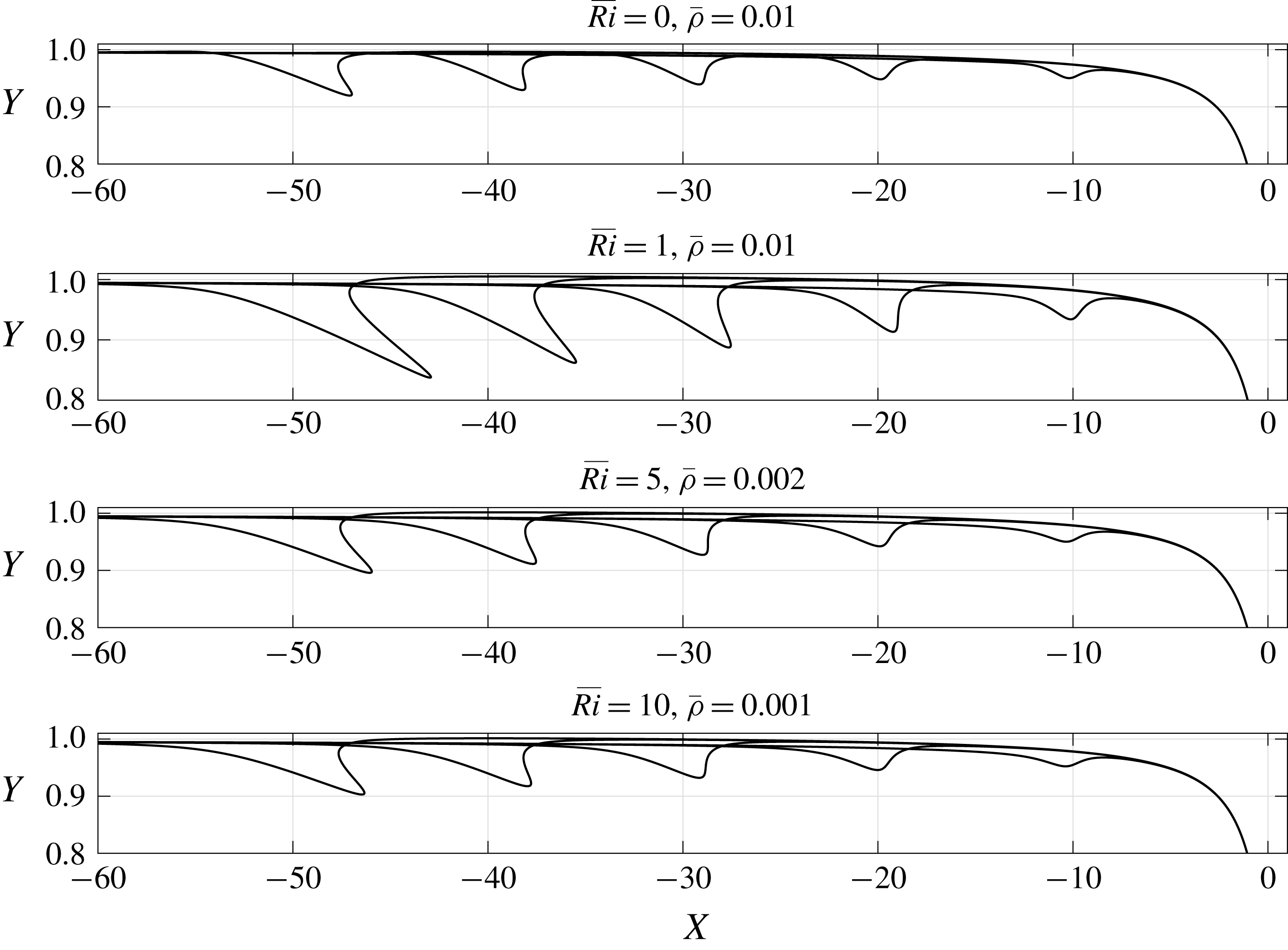
The position of the free surface when
 $t=10$
, 20, 30, 40 and 50 for various values of
 $\bar{Ri}$
and
 $\bar{\unicode[STIX]{x1D70C}}$
, calculated from the asymptotic solution for
 $\bar{\unicode[STIX]{x1D70C}}\ll 1$
. The values of
 $\bar{\unicode[STIX]{x1D70C}}$
are chosen to give deformations of the surface that are neither too small to see clearly, nor too large. Note the unequal scales of the axes.

Figure 3 shows the free surface at later times for various values of
 $\bar{Ri}$
and
 $\bar{\unicode[STIX]{x1D70C}}$
, again calculated using the asymptotic solution for
 $\bar{\unicode[STIX]{x1D70C}}\ll 1$
. The depression of the free boundary can be seen to continue to propagate at unit speed whilst deepening, steepening and eventually overturning (although the position of the free boundary remains a single-valued function
 $r=R_{0}(\unicode[STIX]{x1D703})+\bar{\unicode[STIX]{x1D70C}}\bar{R}(\unicode[STIX]{x1D703},t)$
). The larger the value of
 $\bar{Ri}$
, the deeper the depression (note the different choices of
 $\bar{\unicode[STIX]{x1D70C}}$
in each panel of figure 3). As the depression deepens and the slope of the boundary increases, this linear theory breaks down. As we shall see in § 5, nonlinearity leads to a dispersive shock at the rear of the depression (see figure 10), and the eventual formation of a singularity in the curvature. Ahead of the depression, the free boundary asymptotes to a locally steady solution with thickness larger than that of the original layer. Note however that, as discussed above, for
 $\bar{Ri}>0$
, the position of the free surface is logarithmically singular as
 $y\rightarrow 0$
. The bounded solution computed in this outer region is an artefact of the method that we have used to approximate the integral in (A 18), with rounding error cutting off the singularity. This indicates how easy it is to compute spurious numerical solutions for this problem, since the logarithmic singularity is so weak.
4 The dam-break solution when
$t\ll 1$
,
$\bar{\unicode[STIX]{x1D70C}}=O(1)$
and
$Ri=O(1)$


The solution when
 $t\ll 1$
with
 $\bar{\unicode[STIX]{x1D70C}}=O(1)$
and
 $Ri=O(1)$
consists of two asymptotic regions: an outer region, where the solution is a small perturbation of the initial conditions, and an inner region, close to the point of contact of the free surface with the boundary,
 $y=0$
, where the logarithmic singularity in the outer flow is resolved. In each region, it is most convenient to represent the free surface as
 $x=X(y,t)$
. Note that for this problem, we find that the Boussinesq approximation (
 $\bar{\unicode[STIX]{x1D70C}}=0$
with
 $Ri>0$
) is a singular perturbation. The acceleration of the two fluids in the inner region is crucial in resolving the outer singularity, and if the two fluids are treated as having equal density in the inertial terms in (2.3), this acceleration is not associated with a restoring force. As noted earlier, the flow in the inner region is effectively a two-fluid dam break, and we use the methods developed by King & Needham (Reference King and Needham1994) and Uddin & Needham (Reference Uddin and Needham2015) to determine the asymptotic solution as
 $t\rightarrow 0$
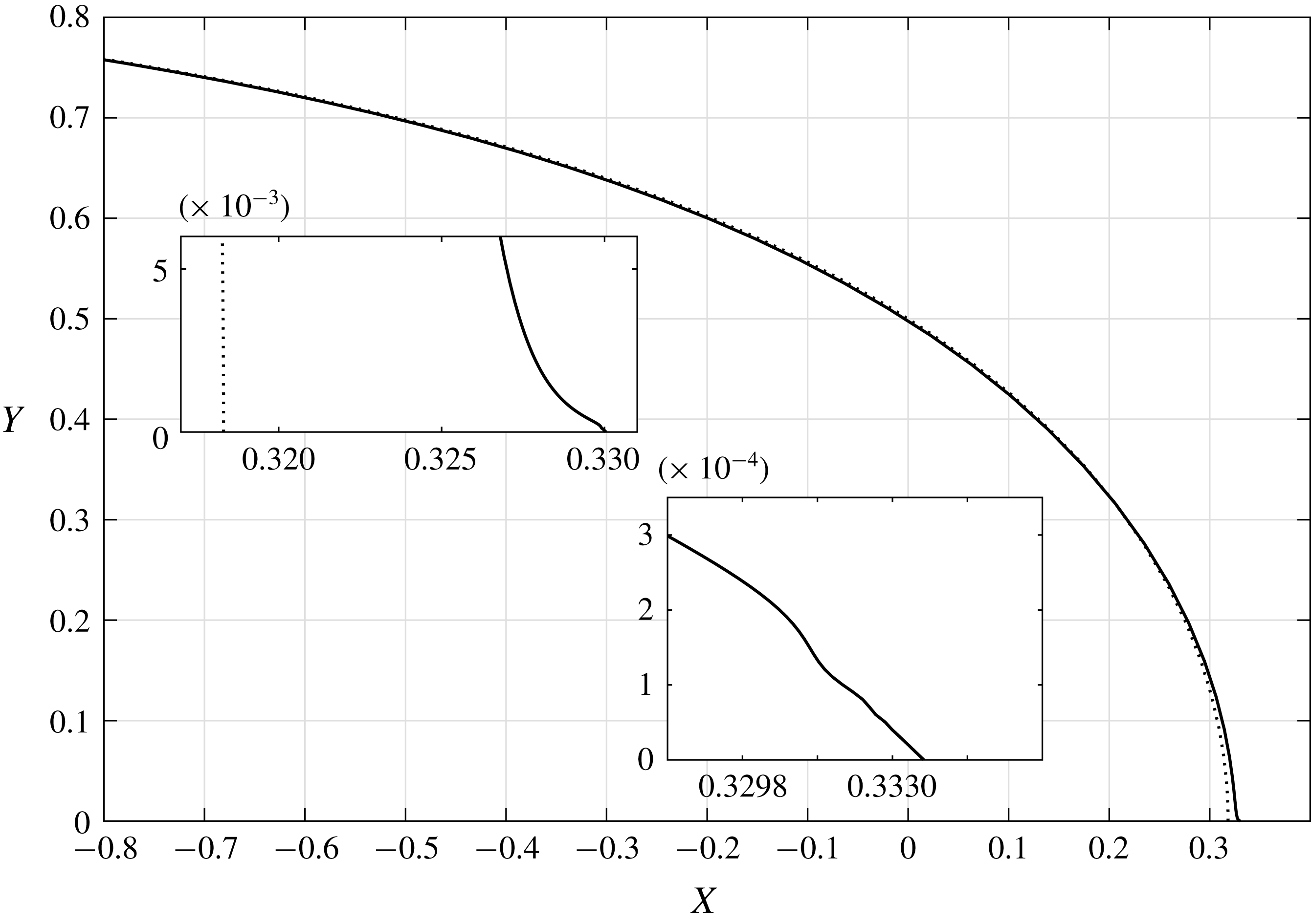
. In addition to the solution in each of two asymptotic regions, constructed and described in appendix B, it is straightforward to construct a composite solution, and figure 4 shows a typical example. Note the huge difference in scales between the main and inset figures, even for the relatively large value,
 $t=0.1$
, which illustrates the complex structure of the asymptotic solution. The displacement of the contact point is of
 $O(t^{2}(-\text{log}\,t))$
as
 $t\rightarrow 0$
, and this singular initial acceleration gives rise to oscillations in the free surface that are of decreasing amplitude and wavelength such that the slope is bounded but the curvature is singular as
 $y\rightarrow 0$
. See appendix B for a more detailed discussion.
The composite asymptotic solution for
 $t\ll 1$
, with
 $\bar{\unicode[STIX]{x1D70C}}=Ri=1$
and
 $t=0.1$
. The dotted line shows the initial position of the free boundary, which meets the solid boundary at
 $x=1/\unicode[STIX]{x03C0}\approx 0.318$
. The insets show close ups of the inner region, close to the contact point.

5 Numerical solution for
$Ri=O(1)$

5.1 Regularisation by a precursor layer
The natural next step in this investigation is to solve the full, nonlinear initial/boundary value problem numerically. We should, however, pause to take stock of what we now know about the behaviour of the solution. We have discovered that, when
 $Ri>0$
, the initial flow near the head of the fluid layer is highly spatially oscillatory and develops in a region with length scale of
 $O(t^{2})$
as
 $t\rightarrow 0$
, with a singular curvature at the contact point. The intricate, multiscale nature of the free surface close to the boundary when
 $t\ll 1$
(see figure 4) means that it is unclear whether it is possible to start a simulation using the asymptotic solution as the initial condition. We did attempt to do this, but were unable to develop a numerically stable solution method. In addition, since the asymptotic solution discussed in § 4 is the leading-order term in an expansion in powers of
 $(-\text{log}\,t)^{-1}$
, its accuracy at times small, and yet large enough to use to initialise a numerical simulation, is low.
In the similar, single fluid dam-break flow studied in Uddin & Needham (Reference Uddin and Needham2015), the inclusion of weak surface tension regularised the solution at small times. This was also the case in the problem studied in Billingham et al. (Reference Billingham, Needham, Korsukova and Munro2017), where a numerical solution showed that the oscillatory small time solution emerges after a short, surface-tension-dominated transient. Whilst we could do the same here, including surface tension is not in the spirit of a simplified problem that is meant to be related to powder snow avalanches, for which the small scale behaviour close to the free boundary is better characterised as particle-laden, multiphase turbulence. We therefore decided, in addition to the regularisation provided by the vortex blob method (see discussion below), to modify the initial condition so that a thin layer of fluid 1 (stationary as
 $x\rightarrow \infty$
in a frame of reference fixed in the solid boundary) lies ahead of the main layer. This is easily achieved by using the streamline given by
 $$\begin{eqnarray}X=Y\cot \unicode[STIX]{x03C0}(Y-\unicode[STIX]{x1D716})\end{eqnarray}$$
as the initial position of the free boundary. In this way, the single fluid solution remains correct when
 $\bar{\unicode[STIX]{x1D70C}}=Ri=0$
, and has
 $Y\rightarrow \unicode[STIX]{x1D716}$
as
 $X\rightarrow \infty$
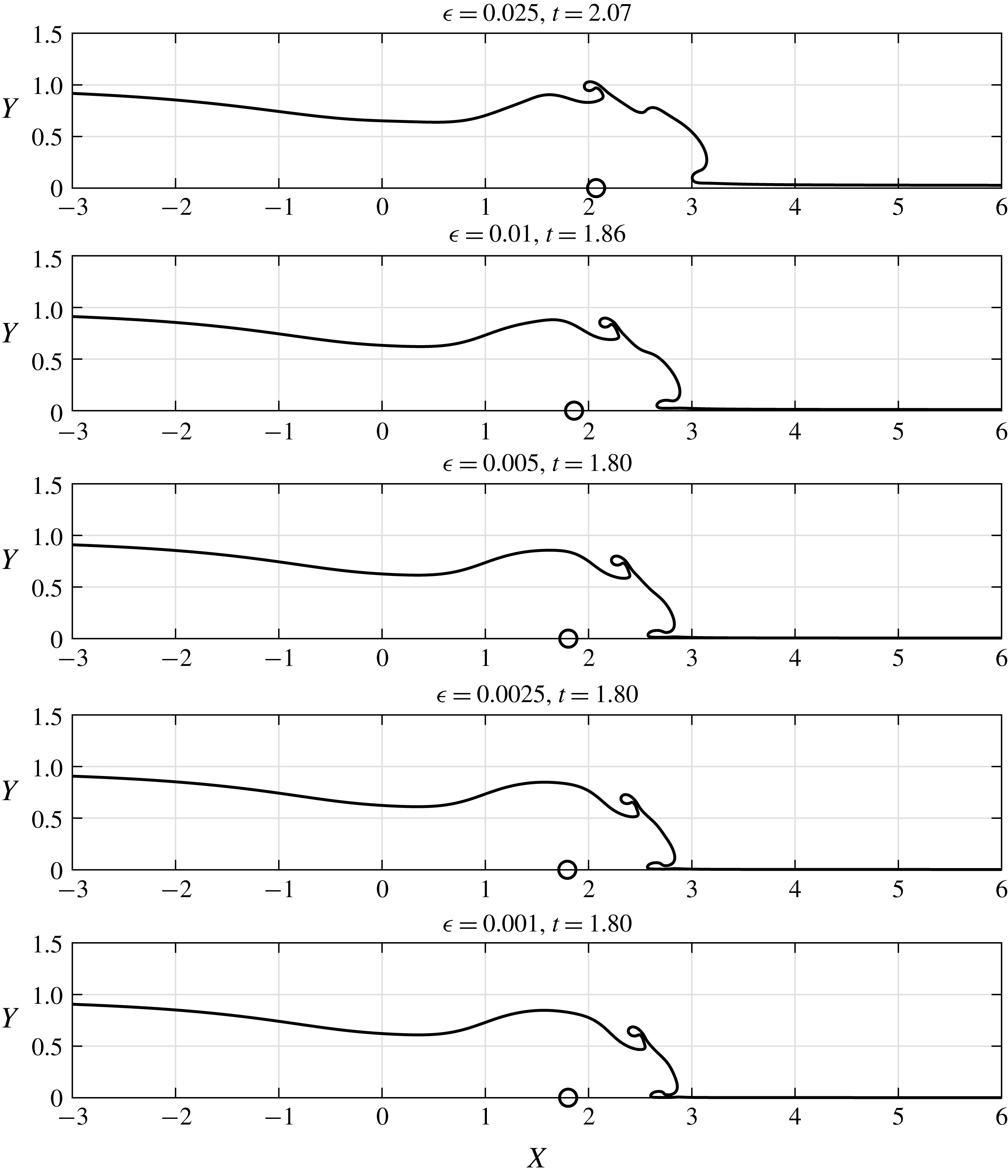
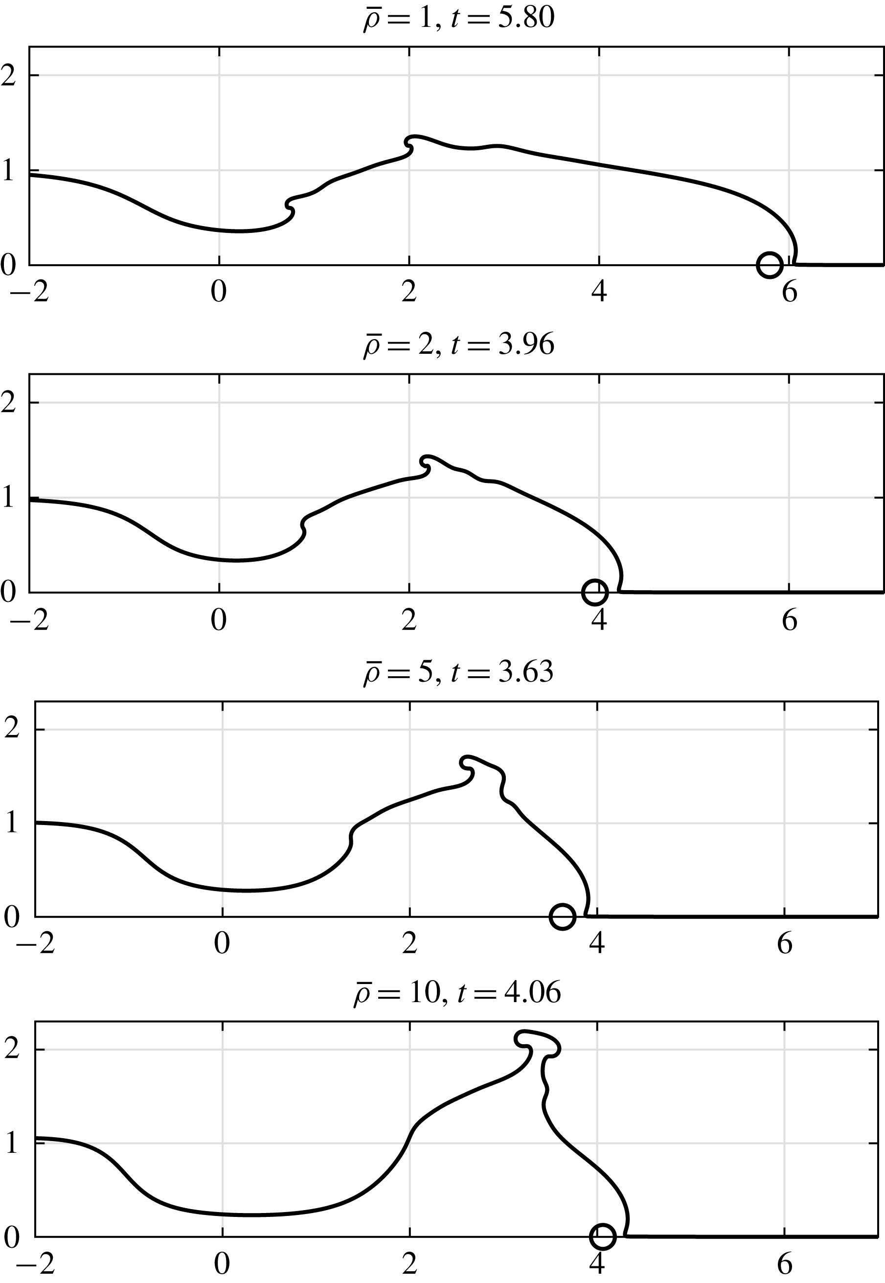
. Figure 5 shows some numerical solutions for the typical case
 $Ri=5$
,
 $\bar{\unicode[STIX]{x1D70C}}=2$
, calculated for a sequence of successively smaller values of
 $\unicode[STIX]{x1D716}$
, in a frame of reference fixed in the boundary, so that the source (shown as a circle) moves to the right at unit speed (see § 5.3 for details of the numerical method used). The features displayed in these simulations, namely a depression of the free surface near the original position of the source, overturning of the upper surface of the layer, and overturning at the head of the layer, are, as we shall see, typical. Note that the stopping criterion was that the number of marker points required for the resolution of the free surface that we used reached 1500, which is a good indicator that the free surface is about to pinch off. Figure 5 provides strong evidence that the value
 $\unicode[STIX]{x1D716}=10^{-3}$
, which we have used in the simulations shown below, is a reasonable choice, as the structure of the flow and the time at which the free surface pinches off appears no longer to be changing as
 $\unicode[STIX]{x1D716}$
decreases past this value. We have not attempted to construct the asymptotic solution in the limit
 $\unicode[STIX]{x1D716}\rightarrow 0$
in this paper.
The numerical solution when
 $Ri=5$
,
 $\bar{\unicode[STIX]{x1D70C}}=2$
and
 $\unicode[STIX]{x1D6FF}=0.05$
for various values of
 $\unicode[STIX]{x1D716}$
at the time just before the free surface pinches off.

Since this regularisation removes the contact point, we can also consider looking for steady solutions. Now
 $Y\rightarrow \unicode[STIX]{x1D716}$
and
 $\unicode[STIX]{x1D719}_{i}\sim -x$
as
 $x\rightarrow \infty$
, so we must modify the Bernoulli constant in (2.4) to give
 $$\begin{eqnarray}(1+\bar{\unicode[STIX]{x1D70C}})\left(\frac{\unicode[STIX]{x2202}\unicode[STIX]{x1D719}_{1}}{\unicode[STIX]{x2202}t}+\frac{1}{2}|\unicode[STIX]{x1D735}\unicode[STIX]{x1D719}_{1}|^{2}\right)-\left(\frac{\unicode[STIX]{x2202}\unicode[STIX]{x1D719}_{2}}{\unicode[STIX]{x2202}t}+\frac{1}{2}|\unicode[STIX]{x1D735}\unicode[STIX]{x1D719}_{2}|^{2}\right)=-Ri(Y-\unicode[STIX]{x1D716})+\frac{1}{2}\bar{\unicode[STIX]{x1D70C}}\quad \text{at}~\boldsymbol{x}=\boldsymbol{X}(s,t).\end{eqnarray}$$
We tried to find steady solutions using a numerical method based on the steady version of that presented below in § 5.3 and continuation from the known solution when
 $\bar{\unicode[STIX]{x1D70C}}=Ri=0$
. We tried continuation in
 $\bar{\unicode[STIX]{x1D70C}}$
,
 $\unicode[STIX]{x1D716}$
and also in an artificial parameter multiplying the source term. We were, however, unable to obtain converged solutions. If we investigate this further by considering the asymptotic solution for
 $\bar{\unicode[STIX]{x1D70C}}\ll 1$
, the equivalents of (A 6) and (A 19) show that now
 $$\begin{eqnarray}\frac{\text{d}\unicode[STIX]{x1D707}}{\text{d}\unicode[STIX]{x1D703}}=\left(\frac{\unicode[STIX]{x1D703}+\unicode[STIX]{x1D716}\unicode[STIX]{x03C0}}{\sin ^{2}\unicode[STIX]{x1D703}}\right)\left(-\bar{Ri}\frac{\unicode[STIX]{x1D703}}{\unicode[STIX]{x03C0}}-\frac{\sin ^{2}\unicode[STIX]{x1D703}}{2(\unicode[STIX]{x1D703}+\unicode[STIX]{x1D716}\unicode[STIX]{x03C0})^{2}}+\frac{\sin \unicode[STIX]{x1D703}\cos \unicode[STIX]{x1D703}}{\unicode[STIX]{x1D703}+\unicode[STIX]{x1D716}\unicode[STIX]{x03C0}}\right),\end{eqnarray}$$
which is of
 $O(\unicode[STIX]{x1D703}^{-1})$
as
 $\unicode[STIX]{x1D703}\rightarrow 0$
. This leads to a non-integrable singularity in the vortex sheet representation, equation (A 18), which shows that a finite solution does not exist, consistent with our failed attempts to use numerical continuation starting from
 $\bar{\unicode[STIX]{x1D70C}}=0$
. All of this strongly suggests that no steady solution of the regularised problem with
 $\unicode[STIX]{x1D716}>0$
exists, and hence that the steady solution
 $\unicode[STIX]{x1D719}_{i}=-x+(1/\unicode[STIX]{x03C0})\log r$
is structurally unstable to small perturbations in the density of the fluid below a streamline. This does not, however, mean that the unsteady solution that evolves from initial conditions based on this special solution are not interesting and of possible relevance to powder snow avalanches.
5.2 The adaptive vortex blob method
It is well known that periodic, two-fluid, inviscid, irrotational flow with a vortex sheet is ill posed (Ebin Reference Ebin1988) and that Moore singularities develop in finite time (Moore Reference Moore1978). When surface tension is included, the singularity is avoided, and instead the free surface forms Kelvin–Helmholtz rolls. Spectrally accurate simulations of this roll-up have been performed on geometrically simple problems with periodic initial conditions, regularised either by surface tension (for example, Hou, Lowengrub & Shelley Reference Hou, Lowengrub and Shelley1994) or by using a vortex blob method (for example, Baker & Pham Reference Baker and Pham2006). We therefore choose to use the latter method, in which the vortex sheet is replaced with a distribution of vorticity.
There are some remarks that we should make that arise from the aperiodic nature of the flow that we are interested in. Firstly, we are not concerned here with the details of the Kelvin–Helmholtz roll-up process. We want to understand the bulk dynamics of the flow, and determine where roll-up starts to occur, but appreciate that the details of the roll-up will depend on the regularisation used. Secondly, in previous work using the vortex blob method, the grid spacing in the periodic domain of solution was constant. We will use an adaptive boundary integral method, with a time-dependent, non-uniform grid size that allows us to resolve regions of the boundary where small scale features develop. We must therefore decide how to choose
 $L_{\unicode[STIX]{x1D6FF}}$
, the length scale over which the vorticity is distributed. We will consider two approaches. In Method 1, we take the length scale to be the grid size,
 $L_{\unicode[STIX]{x1D6FF}}=\unicode[STIX]{x0394}s$
. This is equivalent to a choice taken by Baker & Beale (Reference Baker and Beale2004), which was shown to lead to accurate results for periodic flow without adaptive regridding. In Method 2, we take
 $L_{\unicode[STIX]{x1D6FF}}=\max (\unicode[STIX]{x0394}s,\unicode[STIX]{x1D6FF})$
, with
 $\unicode[STIX]{x1D6FF}>0$
a constant. Here,
 $\unicode[STIX]{x1D6FF}$
is a regularisation parameter that gives the length scale over which vorticity is smeared, which we can think of as a physical quantity that characterises sub-element scale processes, such as turbulence and particle–particle interactions. Using Method 1 (which we note is equivalent to Method 2 with
 $\unicode[STIX]{x1D6FF}=0$
), we are able to compute the development of a Moore singularity up to large curvatures, but, because we adaptively regrid the boundary to resolve the local curvature, the singularity is not removed, and we cannot compute beyond it.
The effect of varying
 $\unicode[STIX]{x1D6FF}$
in the typical example,
 $Ri=5$
,
 $\bar{\unicode[STIX]{x1D70C}}=2$
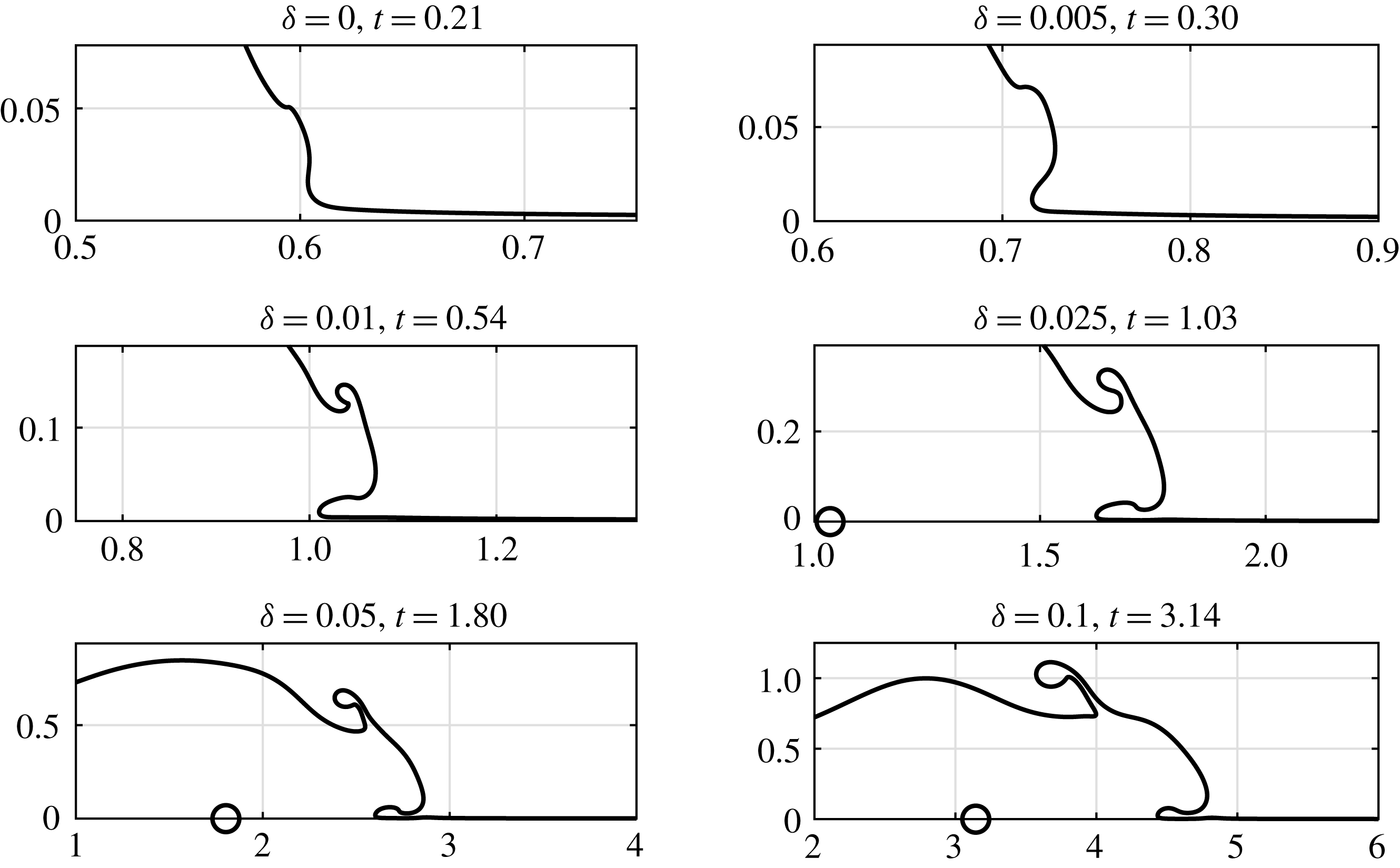
, is shown in figure 6 (note the different scales on the axes). When
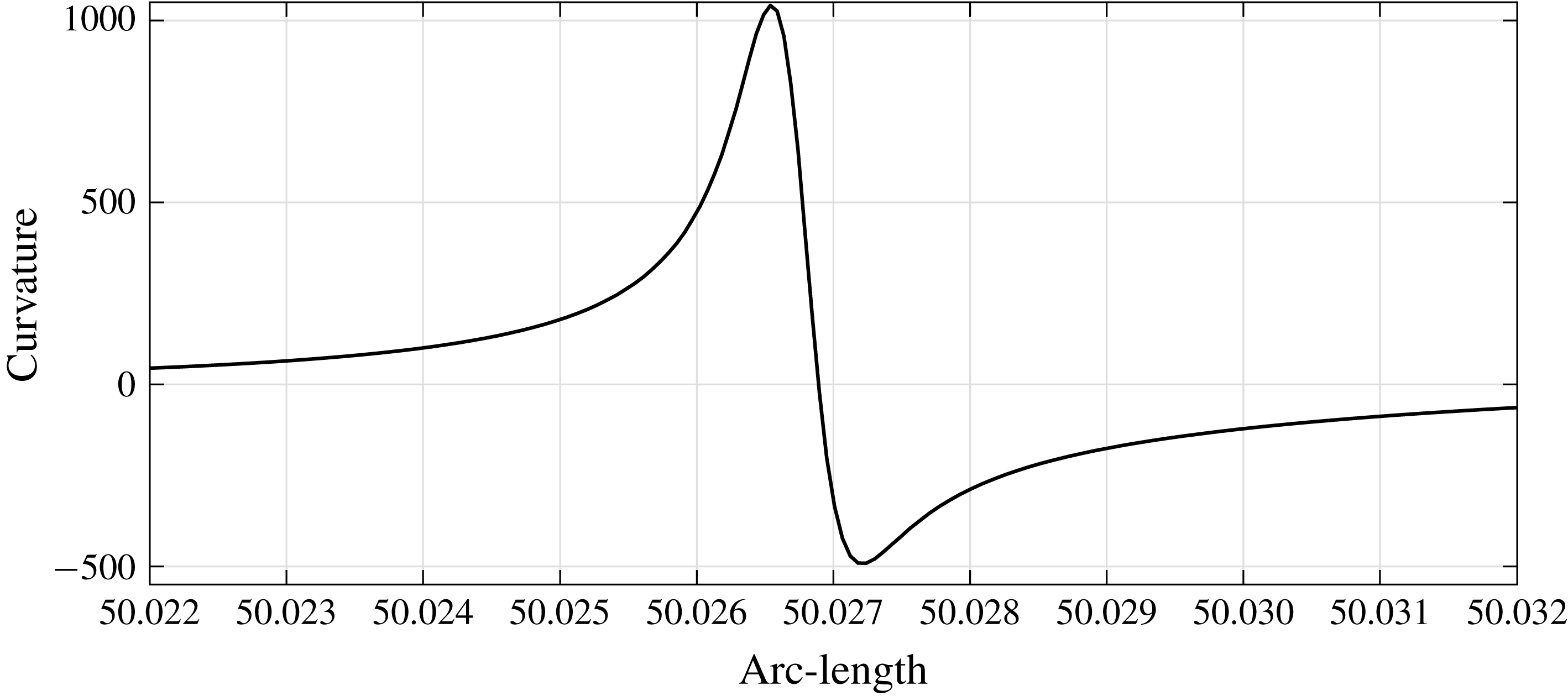
 $\unicode[STIX]{x1D6FF}=0$
, the solution terminates at a developing singularity in the curvature near the head of the layer, as shown in figure 7, where we compute until the curvature reaches 1000. In contrast, using Method 2, the Moore singularity is regularised, so we can integrate beyond its formation time and compute an interface that rolls up and overturns, plotted in figure 6 just before the free surface pinches off. These rolls start to form at the same time and place as in the solution for
 $\unicode[STIX]{x1D6FF}=0$
. As
 $\unicode[STIX]{x1D6FF}$
increases, the onset of overturning is delayed and the length scale of the rolls increases. In the simulations shown below, we have used
 $\unicode[STIX]{x1D6FF}=0.05$
.
The solution for
 $\bar{\unicode[STIX]{x1D70C}}=2$
,
 $Ri=5$
,
 $\unicode[STIX]{x1D716}=10^{-3}$
and various values of
 $\unicode[STIX]{x1D6FF}$
. The solution is plotted in a frame of reference where the outer fluid is initially stationary at infinity and the source (indicated as a small circle) moves to the right at unit speed. Note the different scales for the axes in each panel. The simulation with
 $\unicode[STIX]{x1D6FF}=0$
was terminated when the maximum curvature was greater than 1000, and for
 $\unicode[STIX]{x1D6FF}>0$
, just before pinch off of the interface.

The curvature of the free boundary for the solution with
 $\unicode[STIX]{x1D6FF}=0$
shown in the top left panel of figure 6, close to the developing singularity in the curvature.

5.3 Numerical method
In order to solve the initial/boundary value problem given by (2.2)–(2.8), it is natural to use a boundary integral method. Consider a set of marker points in the boundary,
 $\unicode[STIX]{x2202}{\mathcal{D}}$
, parameterised by
 $\unicode[STIX]{x1D6FC}$
, that move with velocity
 $\boldsymbol{U}\equiv U\boldsymbol{t}+(\boldsymbol{u}\boldsymbol{\cdot }\boldsymbol{n})\boldsymbol{n}$
, so that
 $$\begin{eqnarray}\frac{\text{d}\boldsymbol{X}}{\text{d}t}=\boldsymbol{U},\end{eqnarray}$$
where
 $\text{d}/\text{d}t$
is the Lagrangian time derivative. The normal component of this velocity matches that of the two fluids, but the tangential component is determined, as we shall see below, by specifying the spacing of the surface marker points. We define the unnormalised vortex sheet strength to be
 $\unicode[STIX]{x1D6FE}\equiv \unicode[STIX]{x1D707}_{\unicode[STIX]{x1D6FC}}(\unicode[STIX]{x1D6FC},t)$
. If
 $\unicode[STIX]{x1D6FE}$
is known, the velocity of the fluid is given, using derivatives of the Plemelj formula (B 13), and an image of the free surface in the solid boundary, by
 $$\begin{eqnarray}W=-1+\frac{1}{\unicode[STIX]{x03C0}z}+\frac{1}{2\unicode[STIX]{x03C0}\text{i}}\,\unicode[STIX]{x2A0D}_{-\infty }^{\infty }\unicode[STIX]{x1D6FE}(\unicode[STIX]{x1D6FC},t)\left\{\frac{1}{Z(\unicode[STIX]{x1D6FC},t)-z}-\frac{1}{Z^{\ast }(\unicode[STIX]{x1D6FC},t)-z}\right\}\text{d}\unicode[STIX]{x1D6FC},\end{eqnarray}$$
where
 $z=x+\text{i}y$
,
 $Z(\unicode[STIX]{x1D6FC},t)=X(\unicode[STIX]{x1D6FC},t)+\text{i}Y(\unicode[STIX]{x1D6FC},t)$
,
 $W=u-\text{i}v$
and
 $\boldsymbol{u}=(u,v)$
. The first two terms on the right-hand side of (5.5) are the unit flow and unit source, which means that
 $\unicode[STIX]{x1D6FE}=0$
when
 $t=0$
. Following Baker, Meiron & Orszag (Reference Baker, Meiron and Orszag1982) and Hou et al. (Reference Hou, Lowengrub and Shelley1994), the dynamic boundary condition can be manipulated to find the evolution equation for
 $\unicode[STIX]{x1D6FE}$
, as
 $$\begin{eqnarray}\displaystyle & & \displaystyle \frac{\text{d}\unicode[STIX]{x1D6FE}}{\text{d}t}-\frac{\unicode[STIX]{x2202}}{\unicode[STIX]{x2202}\unicode[STIX]{x1D6FC}}\left\{\frac{\unicode[STIX]{x1D6FE}}{s_{\unicode[STIX]{x1D6FC}}}(U-\boldsymbol{t}\boldsymbol{\cdot }\boldsymbol{W})\right\}\nonumber\\ \displaystyle & & \displaystyle \quad =-\frac{Ri}{1+{\textstyle \frac{1}{2}}\bar{\unicode[STIX]{x1D70C}}}Y_{\unicode[STIX]{x1D6FC}}-\frac{\bar{\unicode[STIX]{x1D70C}}}{1+{\textstyle \frac{1}{2}}\bar{\unicode[STIX]{x1D70C}}}\left\{s_{\unicode[STIX]{x1D6FC}}\boldsymbol{t}\boldsymbol{\cdot }\frac{\text{d}\boldsymbol{W}}{\text{d}t}+\frac{\unicode[STIX]{x2202}}{\unicode[STIX]{x2202}\unicode[STIX]{x1D6FC}}\left(\frac{\unicode[STIX]{x1D6FE}^{2}}{8s_{\unicode[STIX]{x1D6FC}}^{2}}\right)-(U-\boldsymbol{t}\boldsymbol{\cdot }\boldsymbol{W})\boldsymbol{t}\boldsymbol{\cdot }\boldsymbol{W}_{\unicode[STIX]{x1D6FC}}\right\},\qquad\end{eqnarray}$$
where
 $s(\unicode[STIX]{x1D6FC},t)$
is arclength and
 $\boldsymbol{W}$
is the fluid velocity at the interface given by the principal value integral (5.5). Note that
 $\boldsymbol{n}\boldsymbol{\cdot }\boldsymbol{W}$
is continuous at the boundary, but
 $\boldsymbol{t}\boldsymbol{\cdot }\boldsymbol{W}$
is not, and jumps by an amount
 $\unicode[STIX]{x1D6FE}/s_{\unicode[STIX]{x1D6FC}}$
across the boundary. Note also that, since the first step in the lengthy derivation of (5.6) is differentiation of (5.2) with respect to
 $\unicode[STIX]{x1D6FC}$
, the Bernoulli constant does not appear. The Bernoulli constant in (5.2) simply reflects the upstream boundary conditions, which are satisfied by the initial conditions in the evolution problem that we solve here. In all the solutions shown below,
 $\unicode[STIX]{x1D6FE}\rightarrow 0$
as
 $\unicode[STIX]{x1D6FC}\rightarrow \pm \infty$
, as we would expect since the far field is in equilibrium both up- and downstream.
As an aside, this form of the dynamic boundary condition makes it very straightforward to analyse the motion of the contact point,
 $x=X_{c}(t)$
, (which we have avoided in this formulation by taking
 $\unicode[STIX]{x1D716}>0$
) where continuity of both components of the fluid velocity means that
 $U=\boldsymbol{t}\boldsymbol{\cdot }\boldsymbol{W}$
and
 $\unicode[STIX]{x1D6FE}=0$
. Only two terms in (5.6) are therefore non-zero at the contact point, and we obtain
 $$\begin{eqnarray}\frac{\text{d}^{2}X_{c}}{\text{d}t^{2}}=-\frac{Ri}{\bar{\unicode[STIX]{x1D70C}}}\frac{\text{d}Y}{\text{d}X}(0)\quad \text{for}~Ri>0,\end{eqnarray}$$
consistent with the results of § 4, but valid for all
 $t>0$
. This relationship between the acceleration of the contact point and the slope of the free boundary at the point of contact shows that, for non-zero Richardson number, the initial acceleration is infinite when
 $t=0$
, with the results of § 4 giving
 $\text{d}^{2}X_{c}/\text{d}t^{2}=O(-\text{log}\,t)$
as
 $t\rightarrow 0$
. It also shows that any steady solution must have
 $\text{d}Y/\text{d}X=0$
at the contact point, i.e. the free surface must be tangent to the boundary. We have been unable to construct a non-trivial local solution of this nature, which suggests that steady solutions are ruled out by the behaviour of the solution close to the contact point. In terms of physical variables, abusing our notation for one equation,
 $$\begin{eqnarray}\frac{\text{d}^{2}X_{c}}{\text{d}t^{2}}=-g\frac{\text{d}Y}{\text{d}X}(0).\end{eqnarray}$$
Finally, when
 $Ri=0$
, equation (5.6) shows that
 $\text{d}X/\text{d}Y=0$
at
 $s=0$
, i.e. that the free surface is perpendicular to the boundary at the contact point when gravity is negligible.
Following Baker & Beale (Reference Baker and Beale2004), we define a vortex blob method by modifying (5.5) to be
 $$\begin{eqnarray}W=-1+\frac{1}{\unicode[STIX]{x03C0}z}+\frac{1}{2\unicode[STIX]{x03C0}\text{i}}\,\unicode[STIX]{x2A0D}_{-\infty }^{\infty }\unicode[STIX]{x1D6FE}(\unicode[STIX]{x1D6FC},t)\left\{\frac{g(|Z(\unicode[STIX]{x1D6FC},t)-z|/L_{\unicode[STIX]{x1D6FF}})}{Z(\unicode[STIX]{x1D6FC},t)-z}-\frac{g(|Z^{\ast }(\unicode[STIX]{x1D6FC},t)-z|/L_{\unicode[STIX]{x1D6FF}})}{Z^{\ast }(\unicode[STIX]{x1D6FC},t)-z}\right\}\text{d}\unicode[STIX]{x1D6FC}.\end{eqnarray}$$
We use the lowest-order choice of regularisation function,
 $g(r)=1-\text{e}^{-r^{2}}$
, as discussed by Baker & Beale (Reference Baker and Beale2004), since we are not as concerned with the details of the flow after the curvature singularity has been regularised, and because we use a low-order spatial discretisation. We truncate the surface and discretise using Lagrangian markers and linear elements, with
 $X=X_{j}$
,
 $Y=Y_{j}$
,
 $\unicode[STIX]{x1D6FE}=\unicode[STIX]{x1D6FE}_{j}$
and
 $U=U_{j}$
at
 $\unicode[STIX]{x1D6FC}=j$
, for
 $j=1,2,\ldots ,N$
, so that there are
 $4N$
unknowns. The integral in (5.9) is evaluated using four point Gaussian quadrature. The parameter
 $\unicode[STIX]{x1D6FC}$
is taken to be gridpoint number, and all spatial derivatives are calculated using central differences. Timestepping is done using the implicit midpoint method, solving the resulting system of nonlinear algebraic equations using quasi-Newton iteration at each timestep. We find that we can reuse the Jacobian, the calculation of which using finite differences is the main numerical bottleneck in the simulation, over multiple timesteps. Note also that the simple, linear representation of the free surface means that only a small portion of the integral in (5.9) has to be recalculated when finding the Jacobian, significantly speeding up the calculation. We chose to use an implicit timestepping method in order to reduce numerical instability and to be able to time step for accuracy rather than stability. In spite of this, for sufficiently large
 $Ri$
, there is a weak, grid scale instability in
 $\unicode[STIX]{x1D6FE}$
, which we damp using five point smoothing at each timestep (cf. Longuet-Higgins & Cokelet Reference Longuet-Higgins and Cokelet1976). The kinematic and dynamic boundary conditions, equations (5.4) and (5.9) provide
 $3N$
algebraic equations, and we also specify the required element sizes/marker point separations,
 $\unicode[STIX]{x0394}s_{j}$
, using
 $$\begin{eqnarray}(X_{j+1}-X_{j})^{2}+(Y_{j+1}-Y_{j})^{2}=\unicode[STIX]{x0394}s_{j}^{2}\quad \text{for}~j=1,2,\ldots ,N-1.\end{eqnarray}$$
This allows us to control the tangential spacing of the marker points at each timestep, which is possible because we use implicit timestepping and solve for the tangential marker point velocity,
 $U$
. At each timestep we check whether the curvature of the boundary is adequately resolved, and if not, regrid using quintic splines, so that the curvature of the surface is represented by a cubic spline.
We begin our discussion by making a comparison between the asymptotic solution for
 $\bar{\unicode[STIX]{x1D70C}}\ll 1$
, which we discussed in § 3, and the numerical solution of the fully nonlinear free boundary problem.
5.4 Comparison of numerical and asymptotic solutions for small
$\bar{\unicode[STIX]{x1D70C}}$

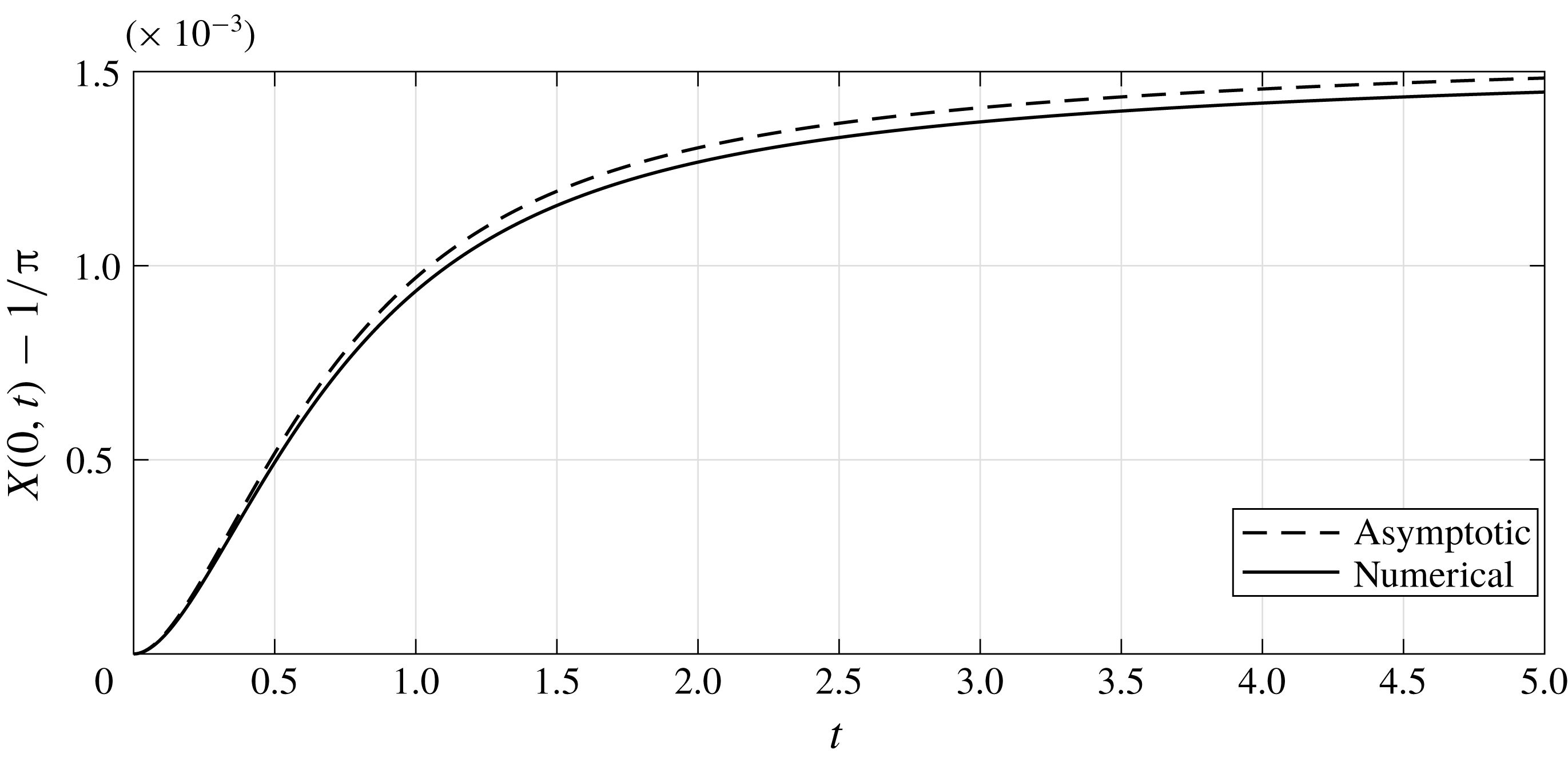
The position of the contact point as a function of time as calculated from the small
 $\bar{\unicode[STIX]{x1D70C}}$
asymptotic and numerical solutions for
 $Ri=0$
and
 $\bar{\unicode[STIX]{x1D70C}}=0.01$
.

The small
 $\bar{\unicode[STIX]{x1D70C}}$
asymptotic (a) and numerical (b) solution for
 $\unicode[STIX]{x1D707}_{s}$
with
 $Ri=0$
and
 $\bar{\unicode[STIX]{x1D70C}}=0.01$
when
 $t=1$
, 2, 3, 4, 5, 10, 15 and 20.

The small
 $\bar{\unicode[STIX]{x1D70C}}$
asymptotic (a) and numerical (b) solutions for
 $Ri=0$
and
 $\bar{\unicode[STIX]{x1D70C}}=0.01$
when
 $t=10$
, 20, 30, 40 and 50. Note the different scales of the axes.

The numerical solution when
 $\bar{\unicode[STIX]{x1D70C}}=0.1$
,
 $Ri=0$
and
 $\unicode[STIX]{x1D6FF}=0.05$
, in a frame of reference fixed in the boundary.

We first consider the solution when
 $Ri=0$
and
 $\bar{\unicode[STIX]{x1D70C}}=0.01$
. Note that when
 $Ri=0$
, there is no initial singularity at the contact point, so we solved the original problem, with no precursor layer (
 $\unicode[STIX]{x1D716}=0$
). Figure 8 shows the position of the contact point as a function of time. The agreement between the asymptotic and numerical solutions is excellent at relatively small times, but has a later discrepancy, which is within the range we would expect given the accuracy of the spatial discretisation of the free boundary in the numerical solution. At times before approximately
 $t=5$
, there is good agreement between the numerical and asymptotic solutions in this case, for both the free surface and
 $\unicode[STIX]{x1D6FE}$
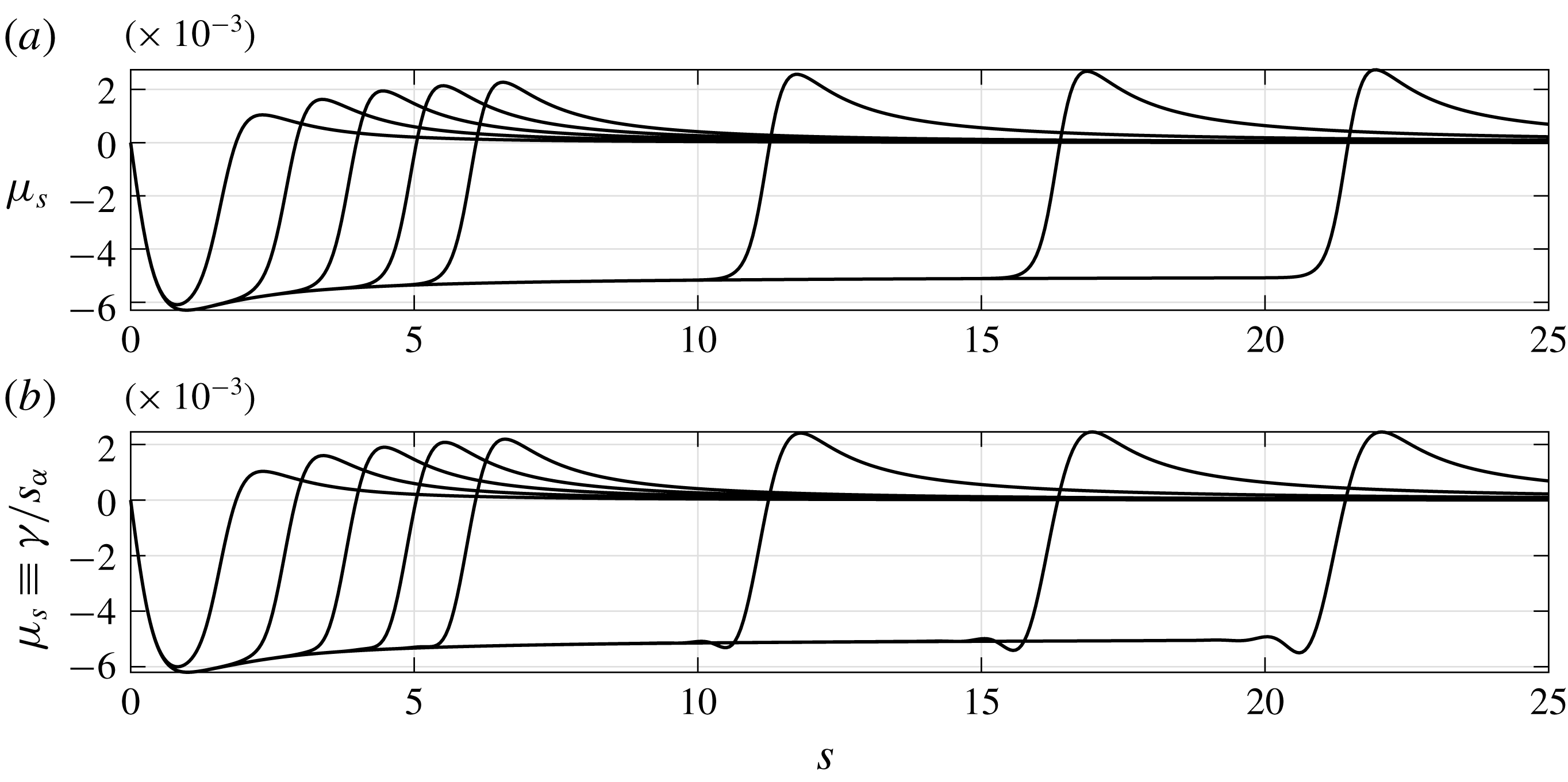
. This can be most clearly seen in figure 9, which shows
 $\unicode[STIX]{x1D707}_{s}\equiv \unicode[STIX]{x1D6FE}/s_{\unicode[STIX]{x1D6FC}}$
at various times up to
 $t=20$
. The agreement between asymptotic and numerical solutions at earlier times is clear. At later times,
 $\unicode[STIX]{x1D707}_{s}$
steepens, as expected, but in addition, oscillations develop, which, within the framework of a weakly nonlinear theory, indicates the formation of a dispersive shock. It should be possible to develop a weakly nonlinear theory, but we have not attempted this here. The comparison between numerical and asymptotic solutions for
 $\unicode[STIX]{x1D707}_{s}$
is a good test of the numerical method, since the asymptotic solution comes from the analytical solution of the simple, semilinear equation (A 6), whilst the numerical solution for
 $\unicode[STIX]{x1D6FE}$
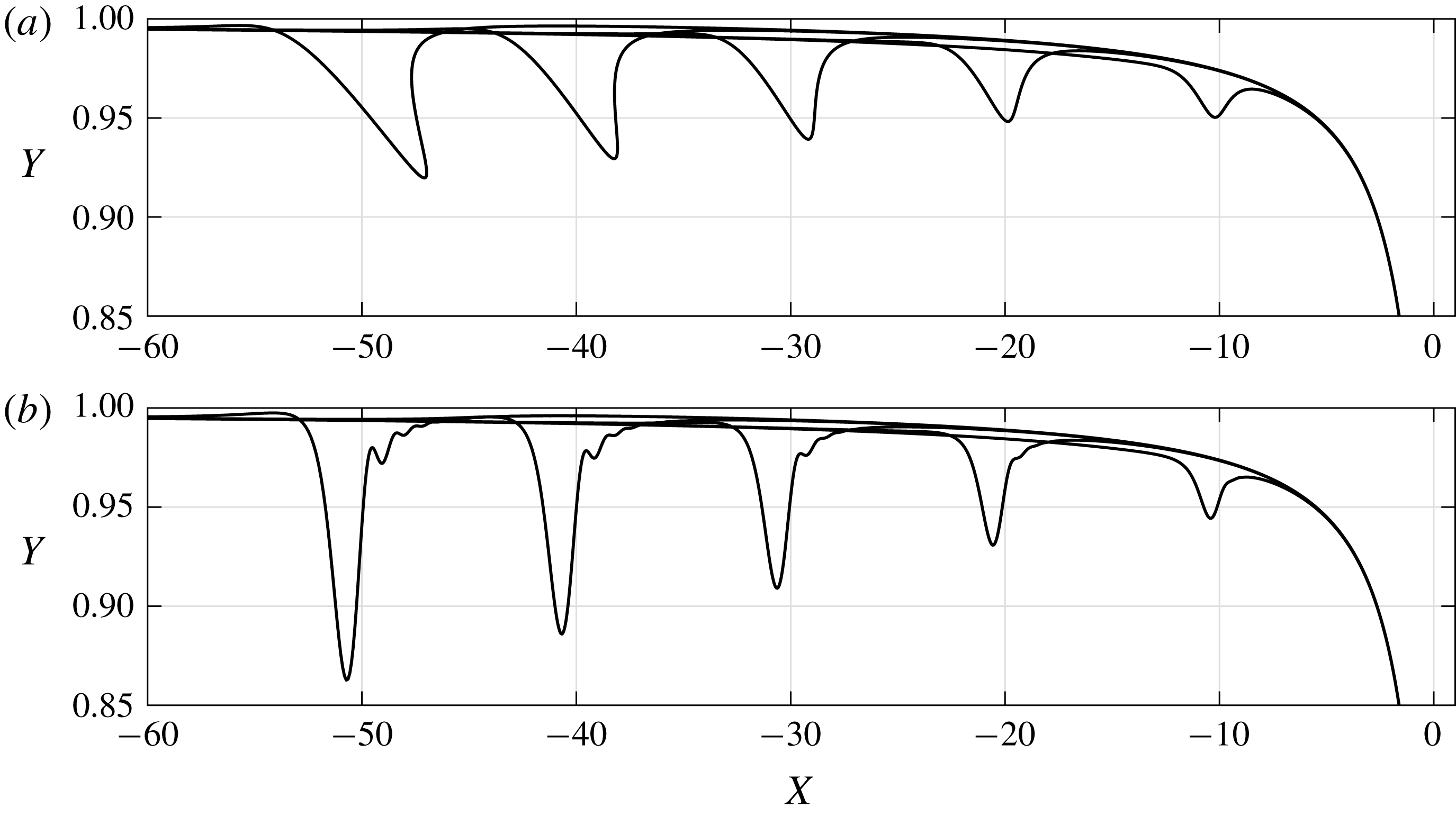
comes from solving the evolution equation (5.6) on the evolving free boundary. Figure 10 shows a comparison of the positions of the free surface at later times, when an increasing discrepancy develops between the asymptotic and numerical solutions. This is due not to discretisation error, but to nonlinearity affecting the deepening depression in the free surface. As the slope of the free surface increases, oscillations form at the rear of the depression, which are coupled to the oscillation in
 $\unicode[STIX]{x1D707}_{s}$
that we can see in figure 9. The numerical solution shown was computed using Method 1, and we expect that it will terminate in a curvature singularity at some later time, beyond the reach of our numerical method. We can however see this occurring for slightly larger
 $\bar{\unicode[STIX]{x1D70C}}$
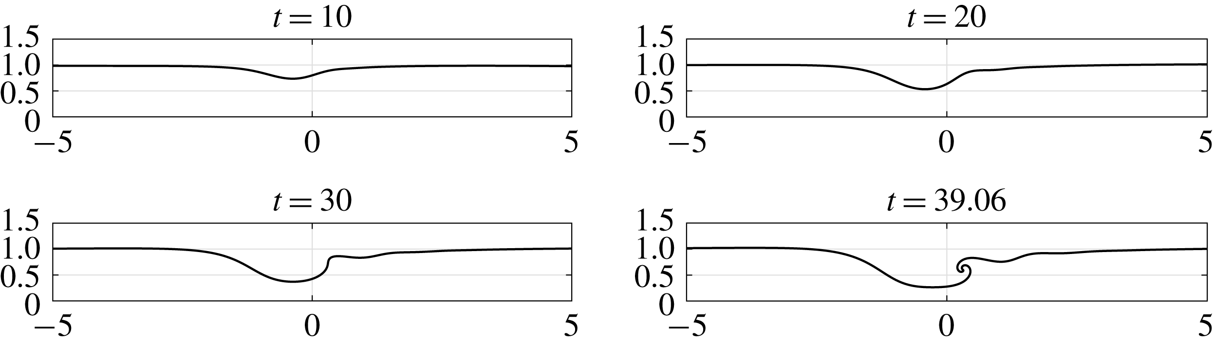
, so we now consider the numerical solution when
 $Ri=0$
and
 $\bar{\unicode[STIX]{x1D70C}}=0.1$
. This value is not particularly small, but leads to behaviour qualitatively similar to the solution for
 $\bar{\unicode[STIX]{x1D70C}}\ll 1$
, as shown in figure 11. For this solution, which was computed with
 $\unicode[STIX]{x1D6FF}=0.05$
, we can also see the depression in the free surface, followed by steepening and the development of a dispersive shock, but now we can solve at times large enough that overturning and the formation of a Kelvin–Helmholtz roll can clearly be seen. Solutions for non-zero values of
 $Ri$
(and
 $\unicode[STIX]{x1D716}=10^{-3}$
) are shown in figure 12. As
 $Ri$
increases, the position of the Kelvin–Helmholtz roll moves towards the head of the flow. Note that for small enough
 $\bar{\unicode[STIX]{x1D70C}}$
, as is the case in figure 12, there is no overturning of the surface at the head of the layer. We should not expect the solutions in figure 12 to agree with the asymptotic solution for
 $\bar{\unicode[STIX]{x1D70C}}\ll 1$
, since this was constructed on the basis that
 $Ri=O(\bar{\unicode[STIX]{x1D70C}})$
.
The numerical solution when
 $\bar{\unicode[STIX]{x1D70C}}=0.1$
and
 $\unicode[STIX]{x1D716}=10^{-3}$
for various values of
 $Ri$
. Note the different scales on the axes.

5.5 Numerical solutions when
$\bar{\unicode[STIX]{x1D70C}}$
is not small

Numerical solutions when
 $Ri=0.1$
for various values of
 $\bar{\unicode[STIX]{x1D70C}}$
.

Numerical solutions when
 $Ri=2$
for various values of
 $\bar{\unicode[STIX]{x1D70C}}$
.

Figures 13–15 show the effect of varying
 $\bar{\unicode[STIX]{x1D70C}}$
with
 $Ri$
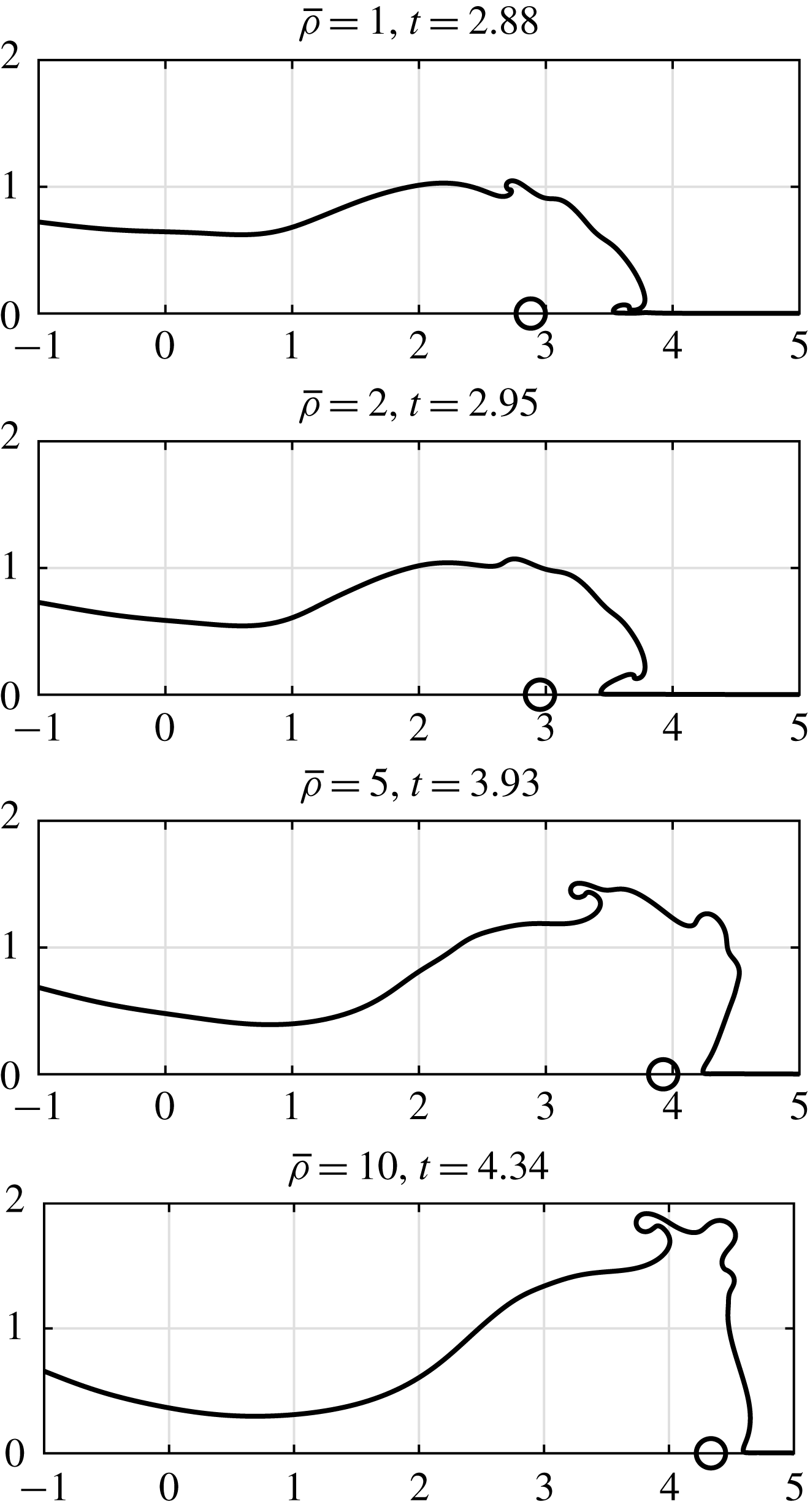
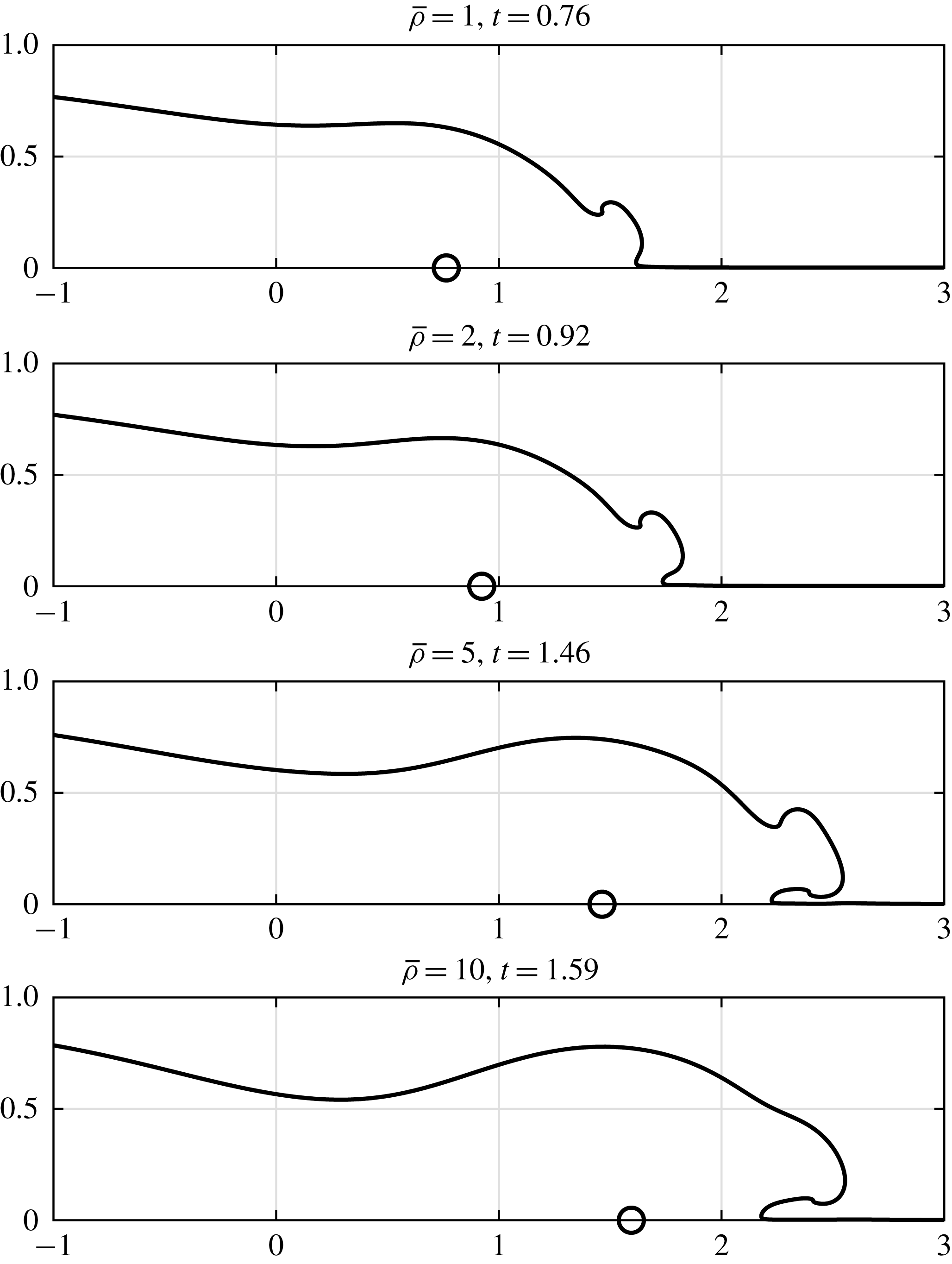
fixed at 0.1, 2 and 10 in successive figures. In each case, we again computed until 1500 marker points were needed to resolve the free surface, which was generally just before pinch off. Movies that show the evolution of the surface for these, and other, combinations of
 $Ri$
and
 $\bar{\unicode[STIX]{x1D70C}}$
are available as Supplementary Material to this paper at https://doi.org/10.1017/jfm.2019.273, as is the MATLAB code used to implement the adaptive vortex blob method. When
 $Ri=0.1$
(figure 13), and hence the effect of gravity is weak, the general tendency is for Kelvin–Helmholtz instability to occur on the upper surface of the layer, with larger values of
 $\bar{\unicode[STIX]{x1D70C}}$
leading to a stronger Bernoulli effect, and fluid being projected upwards more strongly. There is no sign of any overturning at the head of the layer when
 $Ri=0.1$
. When
 $Ri=2$
, and the effect of gravity is stronger (figure 14) overturning can also occur at the head of the layer, but for sufficiently large
 $\bar{\unicode[STIX]{x1D70C}}$
, the initial overturning region is transported along the layer, and fluid is again projected upwards. It is worth noting that the solutions shown in figure 14 do bear some resemblance to the two-dimensional large eddy simulation results presented in figure 6 of Carroll et al. (Reference Carroll, Turnbull and Louge2012), which also suggest that there are large scale bulk motions that are not simply Kelvin–Helmholtz waves. When
 $Ri=10$
(figure 15), and the effect of gravity is even stronger, overturning at the head of the layer is the dominant effect for sufficiently large
 $\bar{\unicode[STIX]{x1D70C}}$
.
Numerical solutions when
 $Ri=10$
for various values of
 $\bar{\unicode[STIX]{x1D70C}}$
.

6 Conclusion
In this paper we have considered the two-dimensional, irrotational flow of a layer of inviscid fluid injected into a different inviscid fluid of lower density by a source on a horizontal boundary moving at constant speed. We were motivated by the work of Carroll et al. (Reference Carroll, Turnbull and Louge2012), which suggests that this flow provides a very simple model for a powder snow avalanche. With this in mind, after finding that the initial, dam-break dynamics gives rise to complex, multiscale behaviour near the intersection point between the fluid layer and the solid boundary, we chose to regularise this motion by including a thin precursor layer ahead of the original fluid layer. In addition, we chose to deal with the Moore singularities that inevitably arise in an inviscid two fluid flow by using a vortex blob method instead of the more usual surface tension regularisation, which is not appropriate in the context of powder snow avalanches. We also introduced an adaptive vortex blob method. This can either be used to integrate up to the formation of a Moore singularity (Method 1,
 $\unicode[STIX]{x1D6FF}=0$
), or, by choosing
 $\unicode[STIX]{x1D6FF}>0$
to be a dimensionless length that characterises small scale processes not modelled by inviscid, irrotational flow, to compute the roll up of the interface on this length scale (Method 2). We found that for small enough dimensionless density difference or Richardson number, the interface rolls up and overturns away from the head of the flow, but that once both the Bernoulli effect and gravity are strong enough, overturning occurs at the head of the layer.
There are some issues that arise from this work, which were mentioned in the paper. Firstly, it would be interesting to derive the weakly nonlinear evolution equation for the free boundary when
 $\bar{\unicode[STIX]{x1D70C}}\ll 1$
and
 $t=O(\bar{\unicode[STIX]{x1D70C}}^{-1})$
, which numerical solutions suggest should describe the formation of a dispersive shock. Secondly, the structure of the asymptotic solution when
 $\unicode[STIX]{x1D716}\ll 1$
, and its relation to the asymptotic solution when
 $\unicode[STIX]{x1D716}=0$
and
 $t\ll 1$
is not clear, and is a challenging problem to try to solve using the method of matched asymptotic expansions. Finally, although it is not relevant to avalanche flows, regularisation of the singular solution when
 $\unicode[STIX]{x1D716}=0$
and
 $t\ll 1$
by the inclusion of surface tension would be of interest in other two-fluid dam-break problems (see Uddin & Needham (Reference Uddin and Needham2015) for the single fluid dam-break problem).
Other extensions to this work that would be of interest in the context of modelling powder snow avalanches include: unsteady one-dimensional modelling of this flow, perhaps using the ideas described in Khodkar, Nasr-Azadani & Meiburg (Reference Khodkar, Nasr-Azadani and Meiburg2017); the use of a level set method to advance the solution beyond the self-intersection time and overcome the main drawback of the boundary integral method that we have used in this paper; including the effect of an underlying slope; adding feedback between the flow and the speed and strength of the source – this is straightforward to include in the existing numerical method, but a sensible model for this feedback needs to be determined, perhaps based on the work of Louge et al. (Reference Louge, Carroll and Turnbull2011), Carroll, Louge & Turnbull (Reference Carroll, Louge and Turnbull2013). In Carroll et al. (Reference Carroll, Louge and Turnbull2013), a steady, one-dimensional model is proposed, with an influx of fresh particulate material prescribed based on a simple model for the cohesive failure of fresh snowpack under the action of the pressure gradient in the eruption current. The challenge is to use these ideas in the context of an unsteady, two-dimensional flow.
Acknowledgements
I’d like to thank my colleagues B. Turnbull (whose work funded by Royal Academy of Engineering award RB4525 gave rise to this idea for modelling powder snow avalanches) and M. Scase for bringing this problem to my attention, and also for helpful discussions and comments on a draft of this paper.
Supplementary movies
Supplementary movies are available at https://doi.org/10.1017/jfm.2019.273.
Appendix A. Asymptotic solution for
$\bar{\unicode[STIX]{x1D70C}}\ll 1$
and
$\bar{Ri}=O(1)$
(see § 3)


When
 $\bar{\unicode[STIX]{x1D70C}}\ll 1$
and
 $\bar{Ri}=O(1)$
, it is most convenient to work in terms of polar coordinates and expand
 $$\begin{eqnarray}R(\unicode[STIX]{x1D703},t)=R_{0}(\unicode[STIX]{x1D703})+\bar{\unicode[STIX]{x1D70C}}\bar{R}(\unicode[STIX]{x1D703},t)+o(\bar{\unicode[STIX]{x1D70C}}),\quad \unicode[STIX]{x1D719}_{i}(r,\unicode[STIX]{x1D703},t)=\unicode[STIX]{x1D719}_{0}(r,\unicode[STIX]{x1D703})+\bar{\unicode[STIX]{x1D70C}}\bar{\unicode[STIX]{x1D719}}_{i}(r,\unicode[STIX]{x1D703},t)+o(\bar{\unicode[STIX]{x1D70C}}),\end{eqnarray}$$
where
 $$\begin{eqnarray}R_{0}(\unicode[STIX]{x1D703})\equiv \frac{\unicode[STIX]{x1D703}}{\unicode[STIX]{x03C0}\sin \unicode[STIX]{x1D703}},\quad \unicode[STIX]{x1D719}_{0}\equiv -r\cos \unicode[STIX]{x1D703}+\frac{1}{\unicode[STIX]{x03C0}}\log r.\end{eqnarray}$$
We begin by studying the dynamics of the vortex sheet strength, which decouples from the rest of the flow in this limit.
A.1 The vortex sheet strength
Note that, since (2.3) includes continuity of normal velocity,
 $\boldsymbol{n}\boldsymbol{\cdot }\unicode[STIX]{x1D735}\unicode[STIX]{x1D719}_{1}=\boldsymbol{n}\boldsymbol{\cdot }\unicode[STIX]{x1D735}\unicode[STIX]{x1D719}_{2}$
at
 $r=R(\unicode[STIX]{x1D703},t)$
, the dynamic boundary condition (2.4) at
 $O(\bar{\unicode[STIX]{x1D70C}})$
is
 $$\begin{eqnarray}\frac{\unicode[STIX]{x2202}\bar{\unicode[STIX]{x1D719}}_{1}}{\unicode[STIX]{x2202}t}-\frac{\unicode[STIX]{x2202}\bar{\unicode[STIX]{x1D719}}_{2}}{\unicode[STIX]{x2202}t}+\frac{1}{2}(\boldsymbol{t}\boldsymbol{\cdot }\unicode[STIX]{x1D735}\unicode[STIX]{x1D719}_{0})^{2}+(\boldsymbol{t}\boldsymbol{\cdot }\unicode[STIX]{x1D735}\unicode[STIX]{x1D719}_{0})(\boldsymbol{t}\boldsymbol{\cdot }\unicode[STIX]{x1D735}\bar{\unicode[STIX]{x1D719}}_{1}-\boldsymbol{t}\boldsymbol{\cdot }\unicode[STIX]{x1D735}\bar{\unicode[STIX]{x1D719}}_{2})=-\bar{Ri}R_{0}\sin \unicode[STIX]{x1D703}\quad \text{at}~r=R_{0}(\unicode[STIX]{x1D703}),\end{eqnarray}$$
where
 $\boldsymbol{t}(s)$
is the unit tangent to the boundary. If we now define
 $$\begin{eqnarray}\unicode[STIX]{x1D707}(\unicode[STIX]{x1D703},t)\equiv \bar{\unicode[STIX]{x1D719}}_{1}(R_{0}(\unicode[STIX]{x1D703}),\unicode[STIX]{x1D703},t)-\bar{\unicode[STIX]{x1D719}}_{2}(R_{0}(\unicode[STIX]{x1D703}),\unicode[STIX]{x1D703},t),\end{eqnarray}$$
(A 3) becomes
 $$\begin{eqnarray}\frac{\unicode[STIX]{x2202}\unicode[STIX]{x1D707}}{\unicode[STIX]{x2202}t}+(\boldsymbol{t}\boldsymbol{\cdot }\unicode[STIX]{x1D735}\unicode[STIX]{x1D719}_{0})\frac{\unicode[STIX]{x2202}\unicode[STIX]{x1D707}}{\unicode[STIX]{x2202}s}=-\bar{Ri}R_{0}\sin \unicode[STIX]{x1D703}-\frac{1}{2}(\boldsymbol{t}\boldsymbol{\cdot }\unicode[STIX]{x1D735}\unicode[STIX]{x1D719}_{0})^{2}\quad \text{at}~r=R_{0}(\unicode[STIX]{x1D703}),\end{eqnarray}$$
and hence, using the known functional forms of
 $R_{0}(\unicode[STIX]{x1D703})$
and
 $\unicode[STIX]{x1D719}_{0}(r,\unicode[STIX]{x1D703})$
,
 $$\begin{eqnarray}\frac{\unicode[STIX]{x2202}\unicode[STIX]{x1D707}}{\unicode[STIX]{x2202}t}+\frac{\unicode[STIX]{x03C0}\sin ^{2}\unicode[STIX]{x1D703}}{\unicode[STIX]{x1D703}}\frac{\unicode[STIX]{x2202}\unicode[STIX]{x1D707}}{\unicode[STIX]{x2202}\unicode[STIX]{x1D703}}=-\bar{Ri}\frac{\unicode[STIX]{x1D703}}{\unicode[STIX]{x03C0}}-\frac{\sin ^{2}\unicode[STIX]{x1D703}-2\unicode[STIX]{x1D703}\sin \unicode[STIX]{x1D703}\cos \unicode[STIX]{x1D703}+\unicode[STIX]{x1D703}^{2}}{2\unicode[STIX]{x1D703}^{2}}.\end{eqnarray}$$
This semilinear equation determines the potential discontinuity across the free surface, and hence the jump in tangential velocity, or vortex sheet strength.
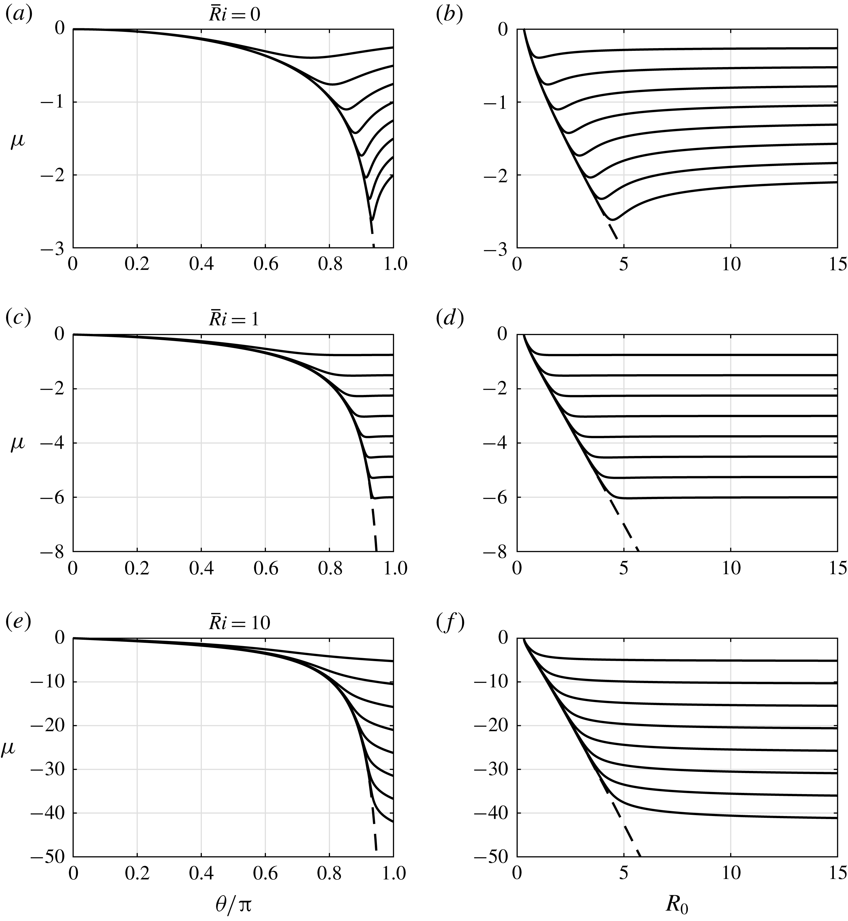
The steady solution of (A 6) is
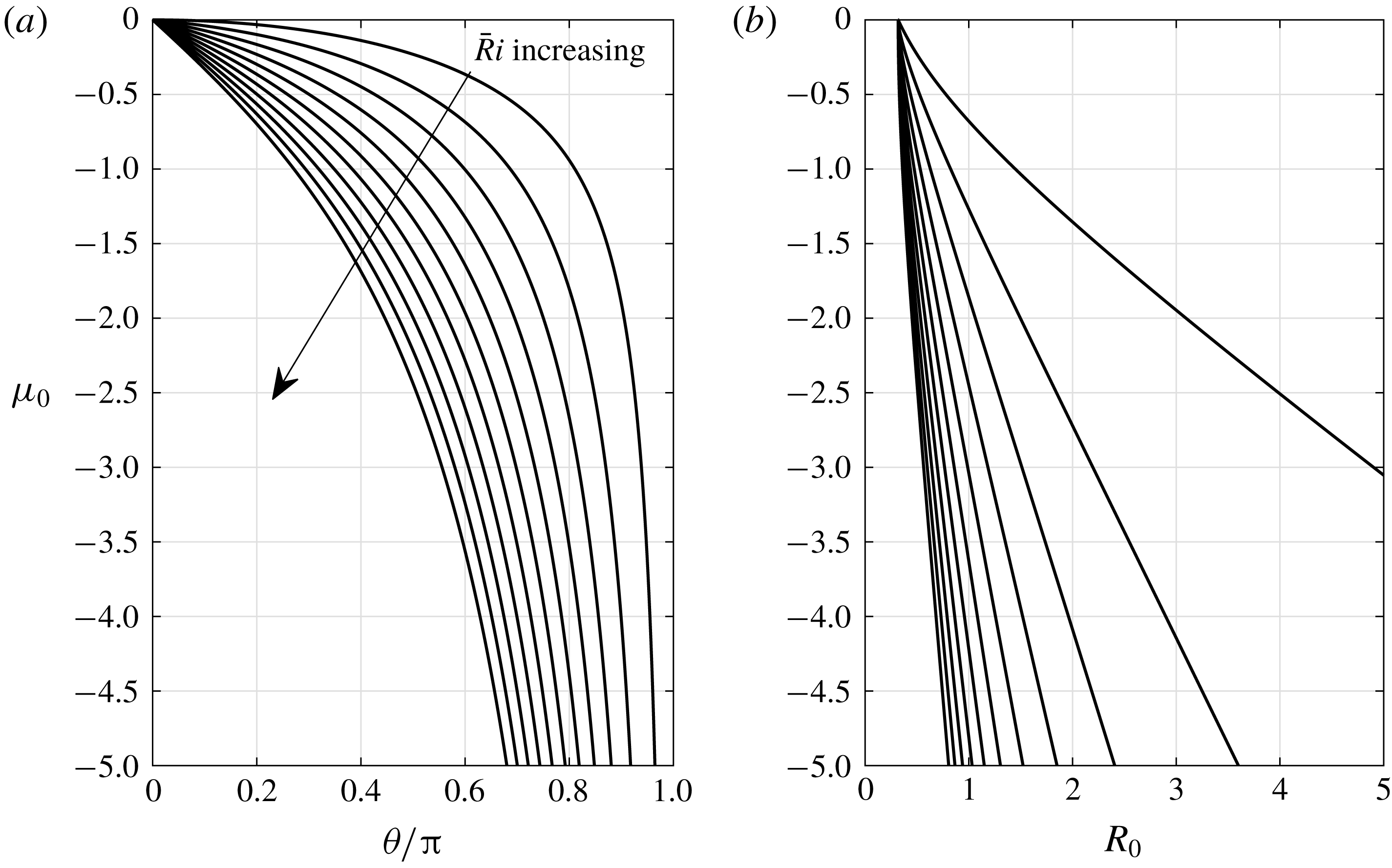
 $$\begin{eqnarray}\unicode[STIX]{x1D707}=\unicode[STIX]{x1D707}_{0}(\unicode[STIX]{x1D703})\equiv \unicode[STIX]{x1D707}_{0}(0)-\frac{\bar{Ri}}{\unicode[STIX]{x03C0}^{2}}\int _{0}^{\unicode[STIX]{x1D703}}\frac{\unicode[STIX]{x1D6FC}^{2}}{\sin ^{2}\unicode[STIX]{x1D6FC}}\,\text{d}\unicode[STIX]{x1D6FC}+\frac{1}{2\unicode[STIX]{x03C0}}\left\{\unicode[STIX]{x1D703}\cot \unicode[STIX]{x1D703}-1+\log \left(\frac{\sin \unicode[STIX]{x1D703}}{\unicode[STIX]{x1D703}}\right)\right\},\end{eqnarray}$$
which is shown for various values of
 $\bar{Ri}$
in figure 16. We find that
 $$\begin{eqnarray}\unicode[STIX]{x1D707}_{0}\sim -\left(\bar{Ri}+\frac{1}{2}\right)\frac{1}{\unicode[STIX]{x03C0}-\unicode[STIX]{x1D703}}-\frac{1}{\unicode[STIX]{x03C0}}\left(2\bar{Ri}-\frac{1}{2}\right)\log (\unicode[STIX]{x03C0}-\unicode[STIX]{x1D703})\quad \text{as}~\unicode[STIX]{x1D703}\rightarrow \unicode[STIX]{x03C0}.\end{eqnarray}$$
Since
 $R_{0}\sim (\unicode[STIX]{x03C0}-\unicode[STIX]{x1D703})^{-1}$
as
 $\unicode[STIX]{x1D703}\rightarrow \unicode[STIX]{x03C0}$
, we can write this as
 $$\begin{eqnarray}\unicode[STIX]{x1D707}_{0}\sim -\left(\bar{Ri}+\frac{1}{2}\right)r+\frac{1}{\unicode[STIX]{x03C0}}\left(2\bar{Ri}-\frac{1}{2}\right)\log r\quad \text{as}~r\rightarrow \infty ,\end{eqnarray}$$
which shows that the jump in tangential velocity tends to
 $\bar{Ri}+1/2$
downstream, as
 $x\rightarrow -\infty$
.
The steady solution,
 $\unicode[STIX]{x1D707}_{0}$
, for
 $\bar{Ri}=0,1,2,\ldots ,10$
, as a function of
 $\unicode[STIX]{x1D703}$
(a) and
 $R_{0}$
(b).

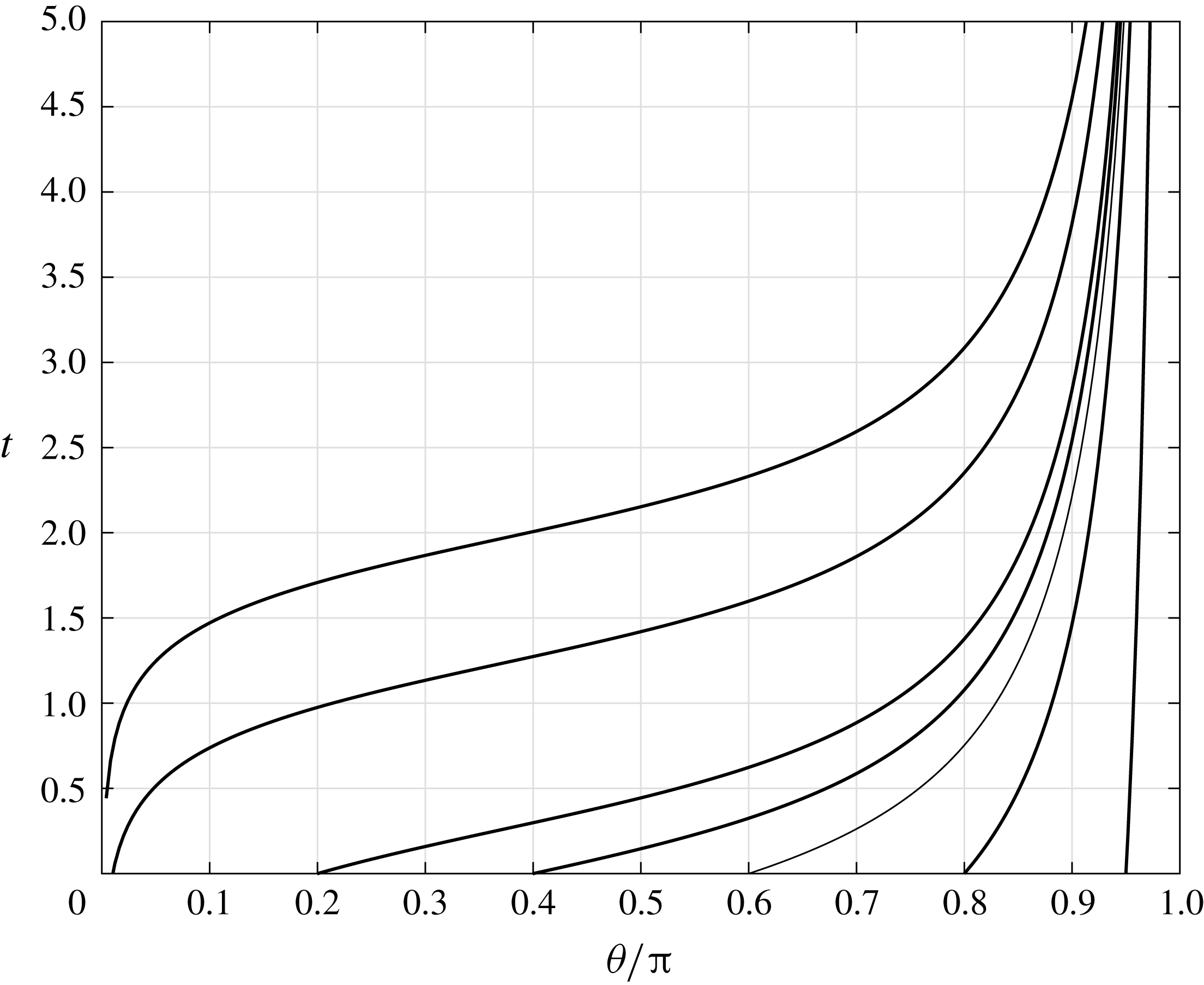
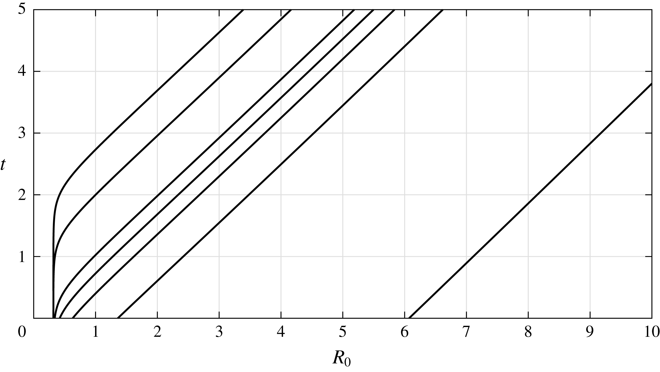
In order to understand the unsteady dynamics of (A 6), note that the solution develops on characteristic curves given by
 $$\begin{eqnarray}\log \sin \unicode[STIX]{x1D703}-\unicode[STIX]{x1D703}\cot \unicode[STIX]{x1D703}=\unicode[STIX]{x03C0}t+\log \sin \unicode[STIX]{x1D703}_{0}-\unicode[STIX]{x1D703}_{0}\cot \unicode[STIX]{x1D703}_{0},\end{eqnarray}$$
which pass through
 $\unicode[STIX]{x1D703}=\unicode[STIX]{x1D703}_{0}$
when
 $t=0$
, as shown in figure 17. Since
 $R_{0}\sim 1/(\unicode[STIX]{x03C0}-\unicode[STIX]{x1D703})$
and
 $\text{d}\unicode[STIX]{x1D703}/\text{d}t\sim (\unicode[STIX]{x03C0}-\unicode[STIX]{x1D703})^{2}$
as
 $\unicode[STIX]{x1D703}\rightarrow \unicode[STIX]{x03C0}$
, we find that, in terms of
 $R_{0}$
, the characteristics have
 $\text{d}R_{0}/\text{d}t\rightarrow 1$
as
 $R_{0}\rightarrow \infty$
, as shown in figure 18. Physically, this means that, away from what we can see in figure 18 is a small neighbourhood of the head of the region occupied by fluid 1 (at
 $x=1/\unicode[STIX]{x03C0}$
,
 $y=0$
), disturbances propagate along the interface at unit speed, which is the dimensionless speed of the source. The closer to
 $x=1/\unicode[STIX]{x03C0}$
the characteristic originates, the longer it remains in its neighbourhood before escaping to infinity, with
 $\unicode[STIX]{x1D703}_{0}\sim \unicode[STIX]{x1D703}\text{e}^{-\unicode[STIX]{x03C0}t}$
as
 $\unicode[STIX]{x1D703}\rightarrow 0$
.
Some characteristic curves of the semilinear equation (A 6).


The solution of (A 6) is then given by
 $$\begin{eqnarray}\unicode[STIX]{x1D707}(\unicode[STIX]{x1D703},t)=\unicode[STIX]{x1D707}(\unicode[STIX]{x1D703}_{0},0)-\frac{\bar{Ri}}{\unicode[STIX]{x03C0}^{2}}\int _{\unicode[STIX]{x1D703}_{0}}^{\unicode[STIX]{x1D703}}\frac{\unicode[STIX]{x1D6FC}^{2}}{\sin ^{2}\unicode[STIX]{x1D6FC}}\,\text{d}\unicode[STIX]{x1D6FC}+\frac{1}{2\unicode[STIX]{x03C0}}\left\{\unicode[STIX]{x1D703}\cot \unicode[STIX]{x1D703}-\unicode[STIX]{x1D703}_{0}\cot \unicode[STIX]{x1D703}_{0}+\log \left(\frac{\unicode[STIX]{x1D703}_{0}\sin \unicode[STIX]{x1D703}}{\unicode[STIX]{x1D703}\sin \unicode[STIX]{x1D703}_{0}}\right)\right\}.\end{eqnarray}$$
The solution with initial condition
 $\unicode[STIX]{x1D707}(\unicode[STIX]{x1D703},0)=0$
is shown in figure 19 for various values of
 $\bar{Ri}$
. It is straightforward to evaluate this accurately for any given values of
 $\unicode[STIX]{x1D703}$
and
 $t$
by solving (A 10) numerically to find
 $\unicode[STIX]{x1D703}_{0}$
and then evaluating (A 11) numerically. The solution can be seen to have two distinct regions:
 $0\leqslant \unicode[STIX]{x1D703}<\unicode[STIX]{x1D703}_{i}(t)$
, in which the solution is given by the steady form
 $\unicode[STIX]{x1D707}=\unicode[STIX]{x1D707}_{0}(\unicode[STIX]{x1D703})$
, and
 $\unicode[STIX]{x1D703}_{i}(t)<\unicode[STIX]{x1D703}\leqslant \unicode[STIX]{x03C0}$
, in which the solution grows with
 $t$
. We can confirm this analytically by considering the large time form of the solution.
The solution,
 $\unicode[STIX]{x1D707}(\unicode[STIX]{x1D703},t)$
, when
 $\unicode[STIX]{x1D707}(\unicode[STIX]{x1D703},0)=0$
and
 $t=0.5$
, 1, 1.5, 2, 2.5, 3, 3.5 and 4, plotted as a function of
 $\unicode[STIX]{x1D703}$
(a) and
 $R_{0}$
(b), for
 $\bar{Ri}=0$
, 1 and 10. The steady state solution is shown as a broken line.

A.2 Solution for
$t\gg 1$

It is clear from (A 10) that when
 $t\gg 1$
,
 $\unicode[STIX]{x1D703}_{0}\ll 1$
and
 $\unicode[STIX]{x1D707}\sim \unicode[STIX]{x1D707}_{0}$
, unless
 $\unicode[STIX]{x1D703}$
is close to
 $\unicode[STIX]{x03C0}$
. By considering the forms of (A 7) and (A 10) when
 $\unicode[STIX]{x03C0}-\unicode[STIX]{x1D703}=O(t^{-1})$
, we find that the asymptotic solution does indeed consist of two distinct regions, separated by a thin, interior layer.
In summary, as
 $t\rightarrow \infty$
,
 $$\begin{eqnarray}\unicode[STIX]{x1D703}_{i}\sim \unicode[STIX]{x03C0}-\frac{1}{t}-\frac{(\log t-1)}{\unicode[STIX]{x03C0}t^{2}},\end{eqnarray}$$
Region I.
 $0\leqslant \unicode[STIX]{x1D703}<\unicode[STIX]{x1D703}_{i}-O(t^{-2})$
.
 $$\begin{eqnarray}\unicode[STIX]{x1D707}=\unicode[STIX]{x1D707}_{0}(\unicode[STIX]{x1D703})+o(1).\end{eqnarray}$$
Region II.
 $|\unicode[STIX]{x1D703}-\unicode[STIX]{x1D703}_{i}|=O(t^{-2})$
.
 $$\begin{eqnarray}\displaystyle & \displaystyle \unicode[STIX]{x1D703}\sim \unicode[STIX]{x1D703}_{i}+\frac{1}{\unicode[STIX]{x03C0}t^{2}}(1+\log \sin \unicode[STIX]{x1D703}_{0}-\unicode[STIX]{x1D703}_{0}\cot \unicode[STIX]{x1D703}_{0}), & \displaystyle\end{eqnarray}$$
 $$\begin{eqnarray}\displaystyle & \displaystyle \unicode[STIX]{x1D707}\sim -\frac{\bar{Ri}}{\unicode[STIX]{x03C0}^{2}}\int _{\unicode[STIX]{x1D703}_{0}}^{\unicode[STIX]{x1D703}_{i}}\frac{\unicode[STIX]{x1D6FC}^{2}}{\sin ^{2}\unicode[STIX]{x1D6FC}}\,\text{d}\unicode[STIX]{x1D6FC}+\frac{1}{2\unicode[STIX]{x03C0}}\left\{\unicode[STIX]{x1D703}\cot \unicode[STIX]{x1D703}-\unicode[STIX]{x1D703}_{0}\cot \unicode[STIX]{x1D703}_{0}+\log \left(\frac{\unicode[STIX]{x1D703}_{0}\sin \unicode[STIX]{x1D703}}{\unicode[STIX]{x1D703}\sin \unicode[STIX]{x1D703}_{0}}\right)\right\}. & \displaystyle\end{eqnarray}$$
Region III.
 $\unicode[STIX]{x1D703}_{i}+O(t^{-2})<\unicode[STIX]{x1D703}\leqslant \unicode[STIX]{x03C0}$
.
 $$\begin{eqnarray}\unicode[STIX]{x1D707}\sim -\left(\bar{Ri}+\frac{1}{2}\right)t-\frac{(\bar{Ri}-1)}{\unicode[STIX]{x03C0}}\log \{1-t(\unicode[STIX]{x03C0}-\unicode[STIX]{x1D703})\}.\end{eqnarray}$$
Note that the solution in Region III shows that the sign of
 $\text{d}\unicode[STIX]{x1D707}/\text{d}\unicode[STIX]{x1D703}$
changes from negative to positive as
 $\bar{Ri}-1$
increases past zero when
 $t\gg 1$
, which can clearly be seen in figure 19, and indicates a change in the nature of the solution in the far field.
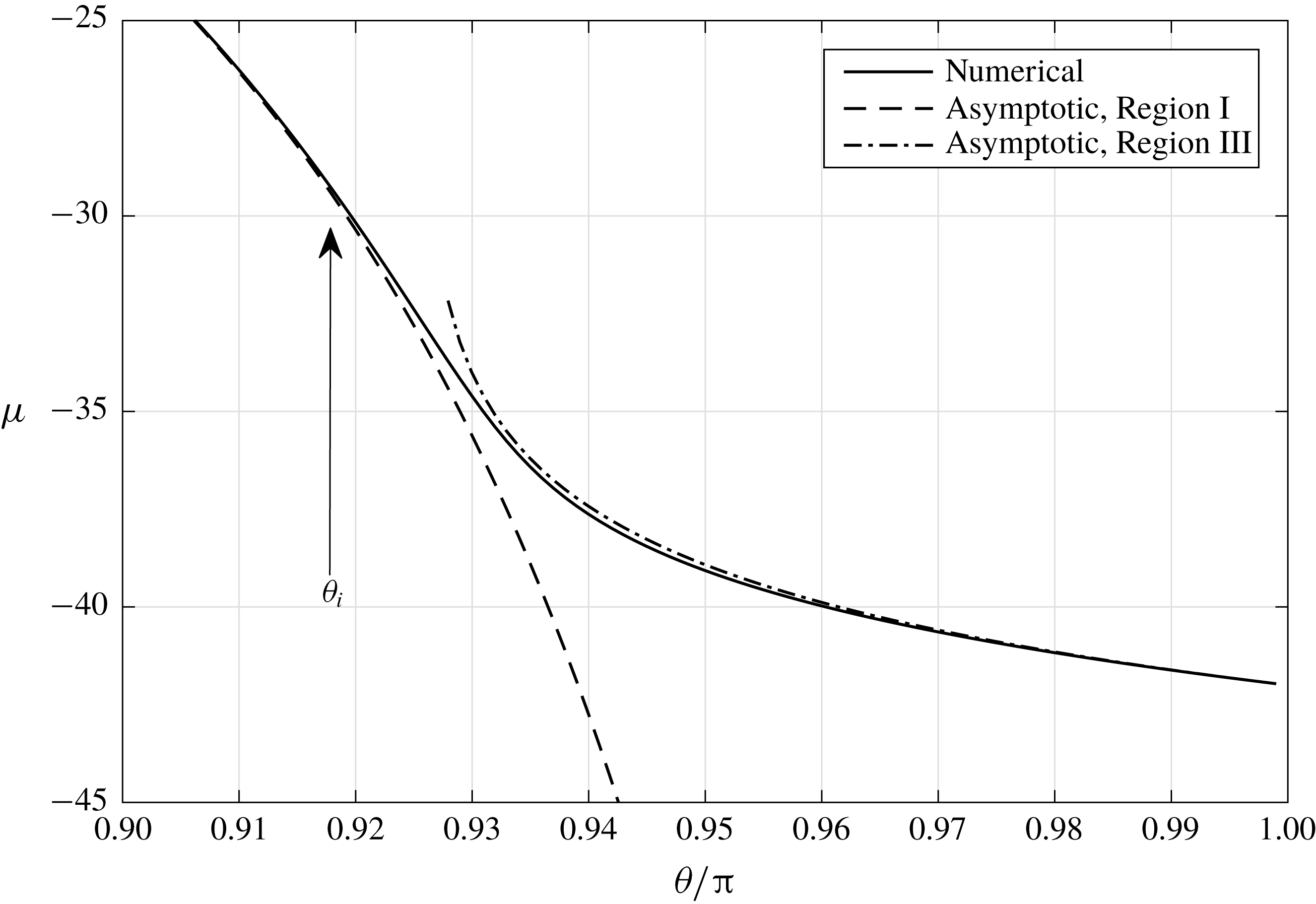
The solution,
 $\unicode[STIX]{x1D707}(\unicode[STIX]{x1D703},t)$
, when
 $\unicode[STIX]{x1D707}(\unicode[STIX]{x1D703},0)=0$
,
 $\bar{Ri}=10$
and
 $t=4$
, along with the asymptotic solution for
 $t\gg 1$
in Regions I and III. The position of the interior layer, at
 $\unicode[STIX]{x1D703}=\unicode[STIX]{x1D703}_{i}$
, is also indicated. The value of
 $\unicode[STIX]{x1D703}_{i}$
is not very accurate for this low value of
 $t$
, but for sufficiently large values of
 $t$
the asymptotic and numerical solutions become indistinguishable.

The asymptotic solution for
 $t\gg 1$
is in excellent agreement with the exact solution, even for low values of
 $t$
. The solution when
 $t=4$
and
 $\bar{Ri}=10$
is shown in figure 20, along with the asymptotic solution in Regions I and III. Far downstream, as
 $r\rightarrow \infty$
,
 $$\begin{eqnarray}\unicode[STIX]{x1D707}\sim -\left(\bar{Ri}+\frac{1}{2}+\frac{\bar{Ri}-1}{\unicode[STIX]{x03C0}R_{0}}\right)t.\end{eqnarray}$$
This shows that the asymptotic expansion (A 1) becomes non-uniform when
 $t=O(\bar{\unicode[STIX]{x1D70C}}^{-1})$
when
 $\bar{\unicode[STIX]{x1D70C}}\ll 1$
, and we expect that the solution becomes nonlinear on this time scale. We will discuss this further in § 5.
A.3 The normal velocity at the free surface,
$\boldsymbol{n}\boldsymbol{\cdot }\unicode[STIX]{x1D735}\bar{\unicode[STIX]{x1D719}}_{1}=\boldsymbol{n}\boldsymbol{\cdot }\unicode[STIX]{x1D735}\bar{\unicode[STIX]{x1D719}}_{2}$

In order to determine the normal velocity at the free surface, which controls its motion, we use the vortex sheet representation (see, for example, Baker et al. Reference Baker, Meiron and Orszag1982),
 $$\begin{eqnarray}\boldsymbol{n}\boldsymbol{\cdot }\unicode[STIX]{x1D735}\bar{\unicode[STIX]{x1D719}}_{i}(s,t)=\frac{1}{2\unicode[STIX]{x03C0}}\boldsymbol{t}(s)\boldsymbol{\cdot }\unicode[STIX]{x2A0D}_{-\infty }^{\infty }\unicode[STIX]{x1D707}_{s}(\unicode[STIX]{x1D703}(s^{\prime }),t)\frac{\boldsymbol{X}(s)-\boldsymbol{X}(s^{\prime })}{|\boldsymbol{X}(s)-\boldsymbol{X}(s^{\prime })|^{2}}\,\text{d}s^{\prime },\end{eqnarray}$$
where
 $\boldsymbol{t}(s)\equiv (X_{s}(s),Y_{s}(s))$
is the unit vector tangent to the boundary and
 $\unicode[STIX]{x1D707}_{s}\equiv \unicode[STIX]{x2202}\unicode[STIX]{x1D707}/\unicode[STIX]{x2202}s$
is the jump in the tangential velocity at the free surface, also known as the normalised vortex sheet strength. We have extended the free surface by reflection in the
 $x$
-axis, with
 $\unicode[STIX]{x1D707}_{s}(-\unicode[STIX]{x1D703},t)=\unicode[STIX]{x1D707}_{s}(\unicode[STIX]{x1D703},t)$
,
 $X(-s)=X(s)$
and
 $Y(-s)=-Y(s)$
by symmetry. The arclength along the fixed boundary can be calculated from
 $$\begin{eqnarray}\frac{\text{d}\unicode[STIX]{x1D703}}{\text{d}s}=\frac{\unicode[STIX]{x03C0}\sin ^{2}\unicode[STIX]{x1D703}}{\sqrt{\sin ^{2}\unicode[STIX]{x1D703}-2\unicode[STIX]{x1D703}\sin \unicode[STIX]{x1D703}\cos \unicode[STIX]{x1D703}+\unicode[STIX]{x1D703}^{2}}}.\end{eqnarray}$$
Equation (A 18) allows us to determine the normal velocity from the vortex sheet strength,
 $\unicode[STIX]{x1D707}_{s}$
, which we discussed above. Note that it is possible to use conformal mapping to find the individual velocity potentials,
 $\bar{\unicode[STIX]{x1D719}}_{1}$
and
 $\bar{\unicode[STIX]{x1D719}}_{2}$
, as integrals of
 $\boldsymbol{n}\boldsymbol{\cdot }\unicode[STIX]{x1D735}\bar{\unicode[STIX]{x1D719}}_{i}$
, but we will not present any details here as it is possible to determine the motion of the free surface from the normal velocity alone.
Figure 21 shows how the vortex sheet strength varies for the same values of time,
 $t$
, used in figure 19. We can see that
 $\unicode[STIX]{x1D707}_{s}$
approaches the steady state solution
 $$\begin{eqnarray}\unicode[STIX]{x1D707}_{0s}(\unicode[STIX]{x1D703})=-\frac{\bar{Ri}\unicode[STIX]{x1D703}^{2}}{\unicode[STIX]{x03C0}\sqrt{\sin ^{2}\unicode[STIX]{x1D703}-2\unicode[STIX]{x1D703}\sin \unicode[STIX]{x1D703}\cos \unicode[STIX]{x1D703}+\unicode[STIX]{x1D703}^{2}}}-\frac{\sqrt{\sin ^{2}\unicode[STIX]{x1D703}-2\unicode[STIX]{x1D703}\sin \unicode[STIX]{x1D703}\cos \unicode[STIX]{x1D703}+\unicode[STIX]{x1D703}^{2}}}{2\unicode[STIX]{x1D703}},\end{eqnarray}$$
in Region I as
 $t$
increases, following the asymptotic solution described in § A.2 even at moderate times. In asymptotic Region III, where
 $R>t-(1/\unicode[STIX]{x03C0})(\log t-1)+O(t^{-1})$
,
 $$\begin{eqnarray}\unicode[STIX]{x1D707}_{s}\sim -\frac{(\bar{Ri}-1)t}{R(R-t)}\quad \text{as}~t\rightarrow \infty .\end{eqnarray}$$
The normalised vortex sheet strength,
 $\unicode[STIX]{x1D707}_{s}$
, when
 $\unicode[STIX]{x1D707}(\unicode[STIX]{x1D703},0)=0$
and
 $t=0.5$
, 1, 1.5, 2, 2.5, 3, 3.5 and 4, the times that are used in figure 19, for
 $\bar{Ri}=0$
, 1 and 10. The broken line shows the steady solution,
 $\unicode[STIX]{x1D707}_{0s}$
, in each case.

In order to determine the behaviour of the free surface, we use the known functional forms of
 $\unicode[STIX]{x1D719}_{0}(r,\unicode[STIX]{x1D703})$
and
 $R_{0}(\unicode[STIX]{x1D703})$
to show that the radial perturbation of the free surface satisfies
 $$\begin{eqnarray}\displaystyle \frac{\unicode[STIX]{x2202}\bar{R}}{\unicode[STIX]{x2202}t}+\frac{\unicode[STIX]{x03C0}\sin ^{2}\unicode[STIX]{x1D703}}{\unicode[STIX]{x1D703}}\frac{\unicode[STIX]{x2202}\bar{R}}{\unicode[STIX]{x2202}\unicode[STIX]{x1D703}} & = & \displaystyle -\frac{\unicode[STIX]{x03C0}\sin \unicode[STIX]{x1D703}\cos \unicode[STIX]{x1D703}}{\unicode[STIX]{x1D703}}\bar{R}\nonumber\\ \displaystyle & & \displaystyle +\,\frac{\sqrt{\sin ^{2}\unicode[STIX]{x1D703}-2\unicode[STIX]{x1D703}\sin \unicode[STIX]{x1D703}\cos \unicode[STIX]{x1D703}+\unicode[STIX]{x1D703}^{2}}}{\unicode[STIX]{x1D703}\sin \unicode[STIX]{x1D703}}\boldsymbol{n}\boldsymbol{\cdot }\unicode[STIX]{x1D735}\bar{\unicode[STIX]{x1D719}_{i}}\quad \text{at}~r=R_{0}(\unicode[STIX]{x1D703}).\qquad\end{eqnarray}$$
In order to solve the simple, linear equation (A 22) numerically, we discretise in
 $\unicode[STIX]{x1D703}$
and approximate
 $\unicode[STIX]{x2202}\bar{R}/\unicode[STIX]{x2202}\unicode[STIX]{x1D703}$
using first-order upwind finite differences. The resulting system of ordinary differential equations can then be solved using ode45 in MATLAB, coupled with the simple initial value problem for
 $\unicode[STIX]{x1D703}_{0}(t;\unicode[STIX]{x1D703})$
,
 $$\begin{eqnarray}\frac{\text{d}\unicode[STIX]{x1D703}_{0}}{\text{d}t}=-\frac{\unicode[STIX]{x03C0}\sin ^{2}\unicode[STIX]{x1D703}_{0}}{\unicode[STIX]{x1D703}_{0}},\quad \text{subject to}~\unicode[STIX]{x1D703}_{0}(0;\unicode[STIX]{x1D703})=\unicode[STIX]{x1D703}.\end{eqnarray}$$
This follows from integrating back along a characteristic at fixed
 $\unicode[STIX]{x1D703}$
, and allows
 $\unicode[STIX]{x1D703}_{0}$
, and hence
 $\unicode[STIX]{x1D707}_{s}$
, to be calculated efficiently as part of the solution. The principal value integral in (A 18) can be evaluated numerically, working in terms of
 $\unicode[STIX]{x1D703}$
, subtracting out the singular behaviour in the neighbourhood of
 $s=s^{\prime }$
(
 $\unicode[STIX]{x1D703}=\unicode[STIX]{x1D703}^{\prime }$
) and using four point Gaussian quadrature. This linear relationship means that the discretised version of
 $\boldsymbol{n}\boldsymbol{\cdot }\unicode[STIX]{x1D735}\unicode[STIX]{x1D719}_{i}$
can be found from
 $\unicode[STIX]{x1D707}_{s}(\unicode[STIX]{x1D703};\unicode[STIX]{x1D703}_{0}(t))$
by multiplication by a constant matrix, which can be precalculated. Some typical solutions are shown in figures 2 and 3.
Appendix B. Asymptotic solution for
$t\ll 1$
(see § 4)

The asymptotic solution for
 $t\ll 1$
can be constructed in terms of an inner and an outer asymptotic region.
B.1 Outer solution:
$\unicode[STIX]{x1D719}_{i}=\unicode[STIX]{x1D719}_{0}+O(t)$
,
$X=X_{0}+O(t^{2})$


We define scaled variables
 $$\begin{eqnarray}\unicode[STIX]{x1D719}_{i}=\unicode[STIX]{x1D719}_{0}(x,y)+t\bar{\unicode[STIX]{x1D719}}_{i}(x,y,t),\quad X=X_{0}(y)+t^{2}\bar{X}(y,t),\end{eqnarray}$$
with
 $\bar{\unicode[STIX]{x1D719}}_{i}$
,
 $\bar{X}=O(1)$
as
 $t\rightarrow 0$
. At leading order, we obtain the boundary value problem
 $$\begin{eqnarray}\unicode[STIX]{x1D6FB}^{2}\bar{\unicode[STIX]{x1D719}}_{i}=0\quad \text{in}~{\mathcal{D}}_{i}(0),\end{eqnarray}$$
subject to
 $$\begin{eqnarray}\displaystyle & \displaystyle \frac{\unicode[STIX]{x2202}\bar{\unicode[STIX]{x1D719}}_{i}}{\unicode[STIX]{x2202}y}=0\quad \text{at}~y=0, & \displaystyle\end{eqnarray}$$
 $$\begin{eqnarray}\displaystyle & \displaystyle (1+\bar{\unicode[STIX]{x1D70C}})\bar{\unicode[STIX]{x1D719}}_{1}-\bar{\unicode[STIX]{x1D719}}_{2}=-Riy-{\textstyle \frac{1}{2}}\bar{\unicode[STIX]{x1D70C}}|\unicode[STIX]{x1D735}\unicode[STIX]{x1D719}_{0}|^{2}\quad \text{at}~x=X_{0}(y), & \displaystyle\end{eqnarray}$$
 $$\begin{eqnarray}\displaystyle & \displaystyle 2\bar{X}=\frac{\unicode[STIX]{x2202}\bar{\unicode[STIX]{x1D719}}_{i}}{\unicode[STIX]{x2202}x}-\frac{\text{d}X_{0}}{\text{d}y}\frac{\unicode[STIX]{x2202}\bar{\unicode[STIX]{x1D719}}_{i}}{\unicode[STIX]{x2202}y}\quad \text{at}~x=X_{0}(y). & \displaystyle\end{eqnarray}$$
Note that
 $\bar{X}(y)$
decouples from the outer problem, and can be determined from (B 5) once the normal velocity at the free surface is known.
B.1.1 Local solution as
$(x-1/\unicode[STIX]{x03C0})^{2}+y^{2}\rightarrow 0$

Close to the point
 $x=1/\unicode[STIX]{x03C0}$
,
 $y=0$
, where the undisturbed free surface meets the boundary (a stagnation point of the initial potential,
 $\unicode[STIX]{x1D719}_{0}(x,y)$
), the incompatibility in the boundary conditions (B 3) and (B 4) leads to a logarithmic singularity, as discussed at the end of § 3. The local solution is
 $$\begin{eqnarray}\displaystyle & \displaystyle \bar{\unicode[STIX]{x1D719}}_{1}\sim p_{0}-\frac{Ri}{\unicode[STIX]{x03C0}\left(1+{\textstyle \frac{1}{2}}\bar{\unicode[STIX]{x1D70C}}\right)}\{r\log r\cos \unicode[STIX]{x1D703}+(\unicode[STIX]{x03C0}-\unicode[STIX]{x1D703})r\sin \unicode[STIX]{x1D703}+kr\cos \unicode[STIX]{x1D703}\}\quad \text{as}~r\rightarrow 0,\quad & \displaystyle\end{eqnarray}$$
 $$\begin{eqnarray}\displaystyle & \displaystyle \bar{\unicode[STIX]{x1D719}}_{2}\sim (1+\bar{\unicode[STIX]{x1D70C}})p_{0}-\frac{Ri}{\unicode[STIX]{x03C0}\left(1+{\textstyle \frac{1}{2}}\bar{\unicode[STIX]{x1D70C}}\right)}\{r\log r\cos \unicode[STIX]{x1D703}-\unicode[STIX]{x1D703}r\sin \unicode[STIX]{x1D703}+kr\cos \unicode[STIX]{x1D703}\}\quad \text{as}~r\rightarrow 0,\quad & \displaystyle\end{eqnarray}$$
where
 $(r,\unicode[STIX]{x1D703})$
is here a set of polar coordinates centred on
 $(1/\unicode[STIX]{x03C0},0)$
, and
 $p_{0}$
and
 $k$
are parameters that are determined globally. Although
 $p_{0}\equiv p_{0}(\unicode[STIX]{x1D70C},\bar{Ri})$
is unimportant,
 $k\equiv k(\bar{\unicode[STIX]{x1D70C}},Ri)$
affects the solution in the inner region. By using (B 7) in (B 5), we find that
 $$\begin{eqnarray}\bar{X}\sim -\frac{Ri}{2\unicode[STIX]{x03C0}\left(1+{\textstyle \frac{1}{2}}\bar{\unicode[STIX]{x1D70C}}\right)}\{\log Y_{0}(s)+1+k\}\quad \text{as}~s\rightarrow 0.\end{eqnarray}$$
It is this logarithmic singularity in the position of the free surface in the outer solution that leads to an inner region where the singularity is resolved.
We will also use the streamfunctions,
 $\bar{\unicode[STIX]{x1D713}}_{1}$
and
 $\bar{\unicode[STIX]{x1D713}}_{2}$
, that correspond to the velocity potentials
 $\bar{\unicode[STIX]{x1D719}}_{1}$
and
 $\bar{\unicode[STIX]{x1D719}}_{2}$
, which have
 $$\begin{eqnarray}\displaystyle & \displaystyle \bar{\unicode[STIX]{x1D713}}_{1}\sim q-\frac{Ri}{\unicode[STIX]{x03C0}\left(1+{\textstyle \frac{1}{2}}\bar{\unicode[STIX]{x1D70C}}\right)}\{r\log r\sin \unicode[STIX]{x1D703}-(\unicode[STIX]{x03C0}-\unicode[STIX]{x1D703})r\cos \unicode[STIX]{x1D703}+kr\sin \unicode[STIX]{x1D703}\}\quad \text{as}~r\rightarrow 0,\quad & \displaystyle\end{eqnarray}$$
 $$\begin{eqnarray}\displaystyle & \displaystyle \bar{\unicode[STIX]{x1D713}}_{2}\sim q-\frac{Ri}{\unicode[STIX]{x03C0}\left(1+{\textstyle \frac{1}{2}}\bar{\unicode[STIX]{x1D70C}}\right)}\{r\log r\sin \unicode[STIX]{x1D703}+\unicode[STIX]{x1D703}r\cos \unicode[STIX]{x1D703}+kr\sin \unicode[STIX]{x1D703}\}\quad \text{as}~r\rightarrow 0.\quad & \displaystyle\end{eqnarray}$$
We will use capital letters with subscripts to denote the potentials and streamfunctions on the boundary as a function of arclength,
 $s$
, and note that
 $$\begin{eqnarray}\unicode[STIX]{x1D6F7}_{1}\sim p_{0}-\frac{Ri}{2\left(1+{\textstyle \frac{1}{2}}\bar{\unicode[STIX]{x1D70C}}\right)}Y_{0}(s),\quad \unicode[STIX]{x1D6F7}_{2}\sim (1+\bar{\unicode[STIX]{x1D70C}})p_{0}+\frac{Ri}{2\left(1+{\textstyle \frac{1}{2}}\bar{\unicode[STIX]{x1D70C}}\right)}Y_{0}(s),\end{eqnarray}$$
 $$\begin{eqnarray}\unicode[STIX]{x1D6F9}_{1}=\unicode[STIX]{x1D6F9}_{2}\equiv \unicode[STIX]{x1D6F9}\sim q-\frac{Ri}{\unicode[STIX]{x03C0}\left(1+{\textstyle \frac{1}{2}}\bar{\unicode[STIX]{x1D70C}}\right)}\{Y_{0}(s)\log Y_{0}(s)+kY_{0}(s)\}\quad \text{as}~s\rightarrow 0.\end{eqnarray}$$
B.1.2 Solution using Plemelj formulae
We define the complex potential,
 $\unicode[STIX]{x1D6F7}(z)=\unicode[STIX]{x1D719}_{i}+\text{i}\unicode[STIX]{x1D713}_{i}$
in
 ${\mathcal{D}}_{i}$
, with
 $z=x+\text{i}y$
, which can be written in terms of the potential difference on the boundary,
 $\unicode[STIX]{x2202}{\mathcal{D}}$
, which we extend into the lower half-plane by symmetry, as
 $$\begin{eqnarray}\unicode[STIX]{x1D6F7}(z)=\frac{1}{2\unicode[STIX]{x03C0}\text{i}}\int _{-\infty }^{\infty }\frac{\unicode[STIX]{x1D6F7}_{1}(s)-\unicode[STIX]{x1D6F7}_{2}(s)}{Z_{0}(s)-z}\frac{\text{d}Z_{0}}{\text{d}s}(s)\,\text{d}s,\end{eqnarray}$$
where
 $Z_{0}(s)\equiv X_{0}(s)+\text{i}Y_{0}(s)$
. On the boundary, the Plemelj formulae (see, for example, Ablowitz & Fokas Reference Ablowitz and Fokas1997) show that
 $$\begin{eqnarray}\unicode[STIX]{x1D6F7}_{1}(s)=\frac{1}{2}(\unicode[STIX]{x1D6F7}_{1}(s)-\unicode[STIX]{x1D6F7}_{2}(s))+\text{Re}\left[\frac{1}{2\unicode[STIX]{x03C0}\text{i}}\,\unicode[STIX]{x2A0D}_{-\infty }^{\infty }\frac{\unicode[STIX]{x1D6F7}_{1}(s^{\prime })-\unicode[STIX]{x1D6F7}_{2}(s^{\prime })}{Z_{0}(s^{\prime })-Z_{0}(s)}\frac{\text{d}Z_{0}}{\text{d}s}(s^{\prime })\,\text{d}s^{\prime }\right].\end{eqnarray}$$
We can now use (B 4) to eliminate
 $\unicode[STIX]{x1D6F7}_{2}$
, and obtain a single Fredholm integral equation of the second kind,
 $$\begin{eqnarray}\displaystyle \unicode[STIX]{x1D6F7}_{1}(s) & = & \displaystyle -\frac{1}{1+{\textstyle \frac{1}{2}}\bar{\unicode[STIX]{x1D70C}}}\left\{\vphantom{\int _{-\infty _{M}}^{\infty ^{M}}}\frac{1}{2}Ri|Y_{0}(s)|\right.\nonumber\\ \displaystyle & & \displaystyle -\left.\text{Re}\left[\frac{1}{2\unicode[STIX]{x03C0}\text{i}}\int _{-\infty }^{\infty }\frac{Ri|Y_{0}(s^{\prime })|+\bar{\unicode[STIX]{x1D70C}}\unicode[STIX]{x1D6F7}_{1}(s^{\prime })+{\textstyle \frac{1}{2}}\bar{\unicode[STIX]{x1D70C}}|\unicode[STIX]{x1D735}\unicode[STIX]{x1D719}_{0}|^{2}}{Z_{0}(s^{\prime })-Z_{0}(s)}\frac{\text{d}Z_{0}}{\text{d}s}(s^{\prime })\,\text{d}s^{\prime }\right]\right\}.\qquad\end{eqnarray}$$
Note that the kernel is regular as
 $s^{\prime }\rightarrow s$
, so this is not a principal value integral. When
 $\bar{\unicode[STIX]{x1D70C}}=0$
, this immediately gives
 $\unicode[STIX]{x1D6F7}_{1}(s)$
, and for
 $\bar{\unicode[STIX]{x1D70C}}>0$
is in a form that can be solved iteratively, using four point Gaussian quadrature to evaluate the integral. In order to determine the displacement of the boundary,
 $\bar{X}$
, note that the streamfunction on the boundary is
 $$\begin{eqnarray}\unicode[STIX]{x1D6F9}(s)=\text{Im}\left[-\frac{1}{2\unicode[STIX]{x03C0}\text{i}}\,\unicode[STIX]{x2A0D}_{-\infty }^{\infty }\frac{Ri|Y_{0}(s^{\prime })|+\bar{\unicode[STIX]{x1D70C}}\unicode[STIX]{x1D6F7}_{1}(s^{\prime })+{\textstyle \frac{1}{2}}\bar{\unicode[STIX]{x1D70C}}|\unicode[STIX]{x1D735}\unicode[STIX]{x1D719}_{0}|^{2}}{Z_{0}(s^{\prime })-Z_{0}(s)}\frac{\text{d}Z_{0}}{\text{d}s}(s^{\prime })\,\text{d}s^{\prime }\right].\end{eqnarray}$$
After regularising this integral and subtracting out the behaviour of
 $\unicode[STIX]{x1D6F7}_{1}(s^{\prime })$
close to
 $s^{\prime }=0$
, which leads to the logarithmic behaviour of
 $\unicode[STIX]{x1D6F9}$
as
 $s\rightarrow 0$
, equation (B 12), we can evaluate
 $\unicode[STIX]{x1D6F9}$
using four point Gaussian quadrature. We can calculate
 $\unicode[STIX]{x2202}\unicode[STIX]{x1D6F9}/\unicode[STIX]{x2202}s=\boldsymbol{n}\boldsymbol{\cdot }\unicode[STIX]{x1D735}\bar{\unicode[STIX]{x1D719}}_{i}$
, and hence the displacement of the boundary,
 $\bar{X}$
, using (B 5). Figure 22 shows the solution for various values of
 $Ri$
and
 $\bar{\unicode[STIX]{x1D70C}}$
, although we have not plotted a point at
 $y=0$
. As expected, there is a logarithmic singularity in
 $\bar{X}(y)$
as
 $y\rightarrow 0$
, but it is too weak to be seen clearly in figure 22. The head of fluid 1 swells and is displaced forwards close to the contact point, reproducing the behaviour that we saw for
 $\bar{\unicode[STIX]{x1D70C}}\ll 1$
and
 $\bar{Ri}=O(1)$
in figure 2. The rate of displacement and size of the swelling increases with
 $\bar{\unicode[STIX]{x1D70C}}$
and
 $Ri$
, but is always qualitatively similar.
The boundary in the small time outer region when
 $Ri=0.1$
, 0.5 and 1 with the values of
 $\bar{\unicode[STIX]{x1D70C}}$
shown when
 $t=0.2$
. The broken line shows the initial position of the boundary.
 $Ri$
increases in the direction of the arrow.

B.2 Inner solution:
$\unicode[STIX]{x1D719}_{i}=O(t^{3}(-\text{log}\,t)^{2})$
,
$x-1/\unicode[STIX]{x03C0}$
,
$y=O(t^{2}(-\text{log}\,t))$


On comparing the size of the terms neglected in the outer region to those retained as
 $s\rightarrow 0$
(equivalently,
 $y\rightarrow 0$
on the boundary), we find that appropriate scaled variables are (see Uddin & Needham (Reference Uddin and Needham2015) for more details on the very similar, single fluid version of this dam-break problem)
 $$\begin{eqnarray}x=\frac{1}{\unicode[STIX]{x03C0}}+Rit^{2}(-\text{log}\,t)\hat{x},\quad y=Rit^{2}(-\text{log}\,t){\hat{y}},\quad X=\frac{1}{\unicode[STIX]{x03C0}}+Rit^{2}(-\text{log}\,t)\hat{X},\end{eqnarray}$$
 $$\begin{eqnarray}\unicode[STIX]{x1D719}_{i}=-\frac{1+\log \unicode[STIX]{x03C0}}{\unicode[STIX]{x03C0}}+Rit^{2}(1+(\text{i}-1)\bar{\unicode[STIX]{x1D70C}})p(\bar{\unicode[STIX]{x1D70C}})+Ri^{2}t^{3}(-\text{log}\,t)^{2}\hat{\unicode[STIX]{x1D719}}_{i},\end{eqnarray}$$
with the hatted variables of
 $O(1)$
as
 $t\rightarrow 0$
. In terms of these, the kinematic and Bernoulli equations, equations (2.3) and (2.4), become
 $$\begin{eqnarray}t\frac{\unicode[STIX]{x2202}\hat{X}}{\unicode[STIX]{x2202}t}+\{2-(-\text{log}\,t)^{-1}\}\left(\hat{X}-{\hat{y}}\frac{\unicode[STIX]{x2202}\hat{X}}{\unicode[STIX]{x2202}{\hat{y}}}\right)=\frac{\unicode[STIX]{x2202}\hat{\unicode[STIX]{x1D719}}_{i}}{\unicode[STIX]{x2202}\hat{x}}-\frac{\unicode[STIX]{x2202}\hat{X}}{\unicode[STIX]{x2202}{\hat{y}}}\frac{\unicode[STIX]{x2202}\hat{\unicode[STIX]{x1D719}}_{i}}{\unicode[STIX]{x2202}{\hat{y}}}\quad \text{at}~\hat{x}=\hat{X},\end{eqnarray}$$
 $$\begin{eqnarray}\displaystyle & & \displaystyle t\frac{\unicode[STIX]{x2202}}{\unicode[STIX]{x2202}t}\{(1+\bar{\unicode[STIX]{x1D70C}})\hat{\unicode[STIX]{x1D719}}_{1}-\hat{\unicode[STIX]{x1D719}}_{2}\}+\{3-2(-\text{log}\,t)^{-1}\}\{(1+\bar{\unicode[STIX]{x1D70C}})\hat{\unicode[STIX]{x1D719}}_{1}-\hat{\unicode[STIX]{x1D719}}_{2}\}\nonumber\\ \displaystyle & & \displaystyle \qquad -\,\{2-(-\text{log}\,t)^{-1}\}\,\hat{\boldsymbol{x}}\boldsymbol{\cdot }\hat{\unicode[STIX]{x1D735}}\{(1+\bar{\unicode[STIX]{x1D70C}})\hat{\unicode[STIX]{x1D719}}_{1}-\hat{\unicode[STIX]{x1D719}}_{2}\}+\frac{1}{2}\{(1+\bar{\unicode[STIX]{x1D70C}})|\hat{\unicode[STIX]{x1D735}}\hat{\unicode[STIX]{x1D719}}_{1}|^{2}-|\hat{\unicode[STIX]{x1D735}}\hat{\unicode[STIX]{x1D719}}_{2}|^{2}\}\nonumber\\ \displaystyle & & \displaystyle \quad =-{\hat{y}}(-\text{log}\,t)^{-1}\quad \text{at}~\hat{x}=\hat{X},\end{eqnarray}$$
and matching with the outer solution requires
 $$\begin{eqnarray}\displaystyle \displaystyle \hat{\unicode[STIX]{x1D719}}_{1} & {\sim} & \displaystyle -\frac{1}{\unicode[STIX]{x03C0}\left(1+{\textstyle \frac{1}{2}}\bar{\unicode[STIX]{x1D70C}}\right)}[\hat{x}\{\log \hat{r}+k(\bar{\unicode[STIX]{x1D70C}})+\log Ri-2(-\text{log}\,t)+\log (-\text{log}\,t)\}+{\hat{y}}(\unicode[STIX]{x03C0}-\hat{\unicode[STIX]{x1D703}})]\nonumber\\ \displaystyle & & \displaystyle \quad \text{as}~\hat{r}\rightarrow \infty ,\end{eqnarray}$$
 $$\begin{eqnarray}\displaystyle \displaystyle \hat{\unicode[STIX]{x1D719}}_{2} & {\sim} & \displaystyle -\frac{1}{\unicode[STIX]{x03C0}\left(1+{\textstyle \frac{1}{2}}\bar{\unicode[STIX]{x1D70C}}\right)}[\hat{x}\{\log \hat{r}+k(\bar{\unicode[STIX]{x1D70C}})+\log Ri-2(-\text{log}\,t)+\log (-\text{log}\,t)\}-{\hat{y}}\hat{\unicode[STIX]{x1D703}}]\nonumber\\ \displaystyle & & \displaystyle \quad \text{as}~\hat{r}\rightarrow \infty ,\end{eqnarray}$$
 $$\begin{eqnarray}\displaystyle \displaystyle \hat{X} & {\sim} & \displaystyle -\frac{1}{2\unicode[STIX]{x03C0}\left(1+{\textstyle \frac{1}{2}}\bar{\unicode[STIX]{x1D70C}}\right)}\{\log {\hat{y}}+k(\bar{\unicode[STIX]{x1D70C}})+1+\log Ri-2(-\text{log}\,t)+\log (-\text{log}\,t)\}\nonumber\\ \displaystyle & & \displaystyle \quad \text{as}~{\hat{y}}\rightarrow \infty .\end{eqnarray}$$
This suggests that we should expand the unknowns as
 $$\begin{eqnarray}\displaystyle & \displaystyle \hat{\unicode[STIX]{x1D719}}_{i}=\hat{\unicode[STIX]{x1D719}}_{i0}+\frac{\log (-\text{log}\,t)}{-\text{log}\,t}\hat{\unicode[STIX]{x1D719}}_{i1}+\frac{1}{-\text{log}\,t}\hat{\unicode[STIX]{x1D719}}_{i2}+o((-\text{log}\,t)^{-1}), & \displaystyle\end{eqnarray}$$
 $$\begin{eqnarray}\displaystyle & \displaystyle \hat{X}=\hat{X}_{0}+\frac{\log (-\text{log}\,t)}{-\text{log}\,t}\hat{X}_{1}+\frac{1}{-\text{log}\,t}\hat{X}_{2}+o((-\text{log}\,t)^{-1}), & \displaystyle\end{eqnarray}$$
with
 $\hat{\unicode[STIX]{x1D719}}_{ij}$
,
 $\hat{X}_{j}=O(1)$
as
 $t\rightarrow 0$
.
On substituting these expansions into (B 19) and (B 20) we find that, although we obtain a fully nonlinear free boundary problem at leading order, there is a simple, linear solution that reproduces the matching conditions up to a constant. A simple linear solution is also available at
 $O(\log (-\text{log}\,t)/(-\text{log}\,t))$
, and we find that
 $$\begin{eqnarray}\displaystyle \hat{\unicode[STIX]{x1D719}}_{i0}=-\frac{1}{\unicode[STIX]{x03C0}\left(1+{\textstyle \frac{1}{2}}\bar{\unicode[STIX]{x1D70C}}\right)}(-2\hat{x}+K_{i}),\quad \hat{X}_{0}=\frac{1}{\unicode[STIX]{x03C0}\left(1+{\textstyle \frac{1}{2}}\bar{\unicode[STIX]{x1D70C}}\right)},\quad (1+\bar{\unicode[STIX]{x1D70C}})K_{1}-K_{2}=\frac{4\bar{\unicode[STIX]{x1D70C}}}{3\unicode[STIX]{x03C0}\left(1+{\textstyle \frac{1}{2}}\bar{\unicode[STIX]{x1D70C}}\right)},\end{eqnarray}$$
 $$\begin{eqnarray}\hat{\unicode[STIX]{x1D719}}_{i1}=-\frac{1}{\unicode[STIX]{x03C0}\left(1+{\textstyle \frac{1}{2}}\bar{\unicode[STIX]{x1D70C}}\right)}(\hat{x}+L_{i}),\quad \hat{X}_{1}=-\frac{1}{2\unicode[STIX]{x03C0}\left(1+{\textstyle \frac{1}{2}}\bar{\unicode[STIX]{x1D70C}}\right)},\quad (1+\bar{\unicode[STIX]{x1D70C}})L_{1}-L_{2}=-\frac{4\bar{\unicode[STIX]{x1D70C}}}{3\unicode[STIX]{x03C0}\left(1+{\textstyle \frac{1}{2}}\bar{\unicode[STIX]{x1D70C}}\right)}.\end{eqnarray}$$
The constants
 $K_{i}$
and
 $L_{i}$
are not fully determined at this order.
At
 $O((-\text{log}\,t)^{-1})$
we obtain a non-trivial boundary value problem set in the quarter planes
 ${\hat{y}}>0$
and
 $\hat{x}<\hat{X}_{0}$
for
 $\hat{\unicode[STIX]{x1D719}}_{12}$
and
 $\hat{x}>\hat{X}_{0}$
for
 $\hat{\unicode[STIX]{x1D719}}_{22}$
. After defining
 $\tilde{\unicode[STIX]{x1D719}}_{i}\equiv \hat{\unicode[STIX]{x1D719}}_{i2}$
,
 $\tilde{X}\equiv \hat{X}_{2}$
,
 $\tilde{x}=\hat{x}-\hat{X}_{0}$
and
 ${\tilde{y}}={\hat{y}}$
, we arrive at
 $$\begin{eqnarray}\displaystyle & \tilde{\unicode[STIX]{x1D6FB}}^{2}\tilde{\unicode[STIX]{x1D719}}_{i}=0\quad \text{in}~\tilde{{\mathcal{D}}}_{i}, & \displaystyle\end{eqnarray}$$
 $$\begin{eqnarray}\displaystyle & \displaystyle 2\tilde{X}-2{\tilde{y}}\frac{\text{d}\tilde{X}}{\text{d}{\tilde{y}}}=\frac{\unicode[STIX]{x2202}\tilde{\unicode[STIX]{x1D719}}_{i}}{\unicode[STIX]{x2202}\tilde{x}}+\frac{1}{\unicode[STIX]{x03C0}\left(1+{\textstyle \frac{1}{2}}\bar{\unicode[STIX]{x1D70C}}\right)}\quad \text{at}~\tilde{x}=0,{\tilde{y}}>0, & \displaystyle\end{eqnarray}$$
 $$\begin{eqnarray}\displaystyle & & \displaystyle 3\{(1+\bar{\unicode[STIX]{x1D70C}})\tilde{\unicode[STIX]{x1D719}}_{1}-\tilde{\unicode[STIX]{x1D719}}_{2}\}-2{\tilde{y}}\frac{\unicode[STIX]{x2202}}{\unicode[STIX]{x2202}{\tilde{y}}}\{(1+\bar{\unicode[STIX]{x1D70C}})\tilde{\unicode[STIX]{x1D719}}_{1}-\tilde{\unicode[STIX]{x1D719}}_{2}\}\nonumber\\ \displaystyle & & \displaystyle \quad =-{\tilde{y}}-\frac{2\bar{\unicode[STIX]{x1D70C}}}{\unicode[STIX]{x03C0}\left(1+{\textstyle \frac{1}{2}}\bar{\unicode[STIX]{x1D70C}}\right)}\tilde{X}-\frac{2\bar{\unicode[STIX]{x1D70C}}}{3\unicode[STIX]{x03C0}^{2}\left(1+{\textstyle \frac{1}{2}}\bar{\unicode[STIX]{x1D70C}}\right)^{2}}\quad \text{at}~\tilde{x}=0,{\tilde{y}}>0,\end{eqnarray}$$
 $$\begin{eqnarray}\displaystyle & \displaystyle \frac{\unicode[STIX]{x2202}\tilde{\unicode[STIX]{x1D719}}_{i}}{\unicode[STIX]{x2202}{\tilde{y}}}=0\quad \text{at}~{\tilde{y}}=0, & \displaystyle\end{eqnarray}$$
 $$\begin{eqnarray}\displaystyle & \displaystyle \tilde{\unicode[STIX]{x1D719}}_{1}\sim -\frac{1}{\unicode[STIX]{x03C0}\left(1+{\textstyle \frac{1}{2}}\bar{\unicode[STIX]{x1D70C}}\right)}[\tilde{x}\{\log \tilde{r}+k(\bar{\unicode[STIX]{x1D70C}})+\log Ri\}+{\tilde{y}}(\unicode[STIX]{x03C0}-\tilde{\unicode[STIX]{x1D703}})]\quad \text{as}~\tilde{r}\rightarrow \infty , & \displaystyle\end{eqnarray}$$
 $$\begin{eqnarray}\displaystyle & \displaystyle \tilde{\unicode[STIX]{x1D719}}_{2}\sim -\frac{1}{\unicode[STIX]{x03C0}\left(1+{\textstyle \frac{1}{2}}\bar{\unicode[STIX]{x1D70C}}\right)}[\tilde{x}\{\log \tilde{r}+k(\bar{\unicode[STIX]{x1D70C}})+\log Ri\}-{\tilde{y}}\tilde{\unicode[STIX]{x1D703}}]\quad \text{as}~\tilde{r}\rightarrow \infty , & \displaystyle\end{eqnarray}$$
 $$\begin{eqnarray}\displaystyle & \displaystyle \tilde{X}\sim -\frac{1}{2\unicode[STIX]{x03C0}\left(1+{\textstyle \frac{1}{2}}\bar{\unicode[STIX]{x1D70C}}\right)}\{\log {\tilde{y}}+k(\bar{\unicode[STIX]{x1D70C}})+1+\log Ri\}\quad \text{as}~{\tilde{y}}\rightarrow \infty . & \displaystyle\end{eqnarray}$$
Note that, at this order in
 $(-\text{log}\,t)^{-1}$
, the inner region does not see the leading-order flow,
 $\unicode[STIX]{x1D719}_{0}(x,y)$
, in these matching conditions, since
 $\unicode[STIX]{x1D719}_{0}$
is quadratic in
 $r$
as
 $r\rightarrow 0$
close to the stagnation point. This is why this inner problem is equivalent to that for a two-fluid dam-break problem, with initially stationary fluids.
A key feature of this boundary value problem is the term involving
 $\bar{\unicode[STIX]{x1D70C}}\tilde{X}$
on the right-hand side of (B 30). This is the reason that the limit
 $\bar{\unicode[STIX]{x1D70C}}\rightarrow 0$
is singular. It is this term, which arises from the inertial terms in the Bernoulli equation in this accelerating inner region, that allows a bounded solution to exist. Simply differentiating (B 30) with respect to
 ${\tilde{y}}$
, taking the limit
 ${\tilde{y}}\rightarrow 0$
and using (B 31) shows that
 $$\begin{eqnarray}\frac{\unicode[STIX]{x2202}\tilde{X}}{\unicode[STIX]{x2202}{\tilde{y}}}(0)=-\frac{\unicode[STIX]{x03C0}\left(1+{\textstyle \frac{1}{2}}\bar{\unicode[STIX]{x1D70C}}\right)}{2\bar{\unicode[STIX]{x1D70C}}}.\end{eqnarray}$$
In terms of the original variables, this is
 $$\begin{eqnarray}\frac{\unicode[STIX]{x2202}X}{\unicode[STIX]{x2202}y}(0)\sim -\frac{\unicode[STIX]{x03C0}\left(1+{\textstyle \frac{1}{2}}\bar{\unicode[STIX]{x1D70C}}\right)}{2\bar{\unicode[STIX]{x1D70C}}(-\text{log}\,t)}\quad \text{as}~t\rightarrow 0,\end{eqnarray}$$
which reproduces the result of King & Needham (Reference King and Needham1994) and Uddin & Needham (Reference Uddin and Needham2015) in the single fluid limit,
 $\bar{\unicode[STIX]{x1D70C}}\rightarrow \infty$
. Note that it is also possible to recover (3.28)–(3.31) with
 $\unicode[STIX]{x1D70E}=1$
in Uddin & Needham (Reference Uddin and Needham2015) in this limit after a rescaling. In the Boussinesq limit,
 $\bar{\unicode[STIX]{x1D70C}}\rightarrow 0$
with
 $Ri=O(1)$
, the slope at the contact point and, as we shall see, its position, tend to infinity, and hence this limit is a singular perturbation.
B.3 Solution of (B 28) to (B 33) using Mellin transforms
We begin by making two transformations of the dependent variables,
 $\tilde{\unicode[STIX]{x1D719}}_{1}$
,
 $\tilde{\unicode[STIX]{x1D719}}_{2}$
and
 $\tilde{X}$
. Firstly, we subtract off the solution at infinity, and rewrite (B 28)–(B 33) in terms of
 $$\begin{eqnarray}\displaystyle & \displaystyle \bar{\unicode[STIX]{x1D719}}_{1}=\tilde{\unicode[STIX]{x1D719}}_{1}+\frac{1}{\unicode[STIX]{x03C0}\left(1+{\textstyle \frac{1}{2}}\bar{\unicode[STIX]{x1D70C}}\right)}[\tilde{x}\{\log \tilde{r}+k(\bar{\unicode[STIX]{x1D70C}})+\log Ri\}+{\tilde{y}}(\unicode[STIX]{x03C0}-\tilde{\unicode[STIX]{x1D703}})], & \displaystyle\end{eqnarray}$$
 $$\begin{eqnarray}\displaystyle & \displaystyle \bar{\unicode[STIX]{x1D719}}_{2}=\tilde{\unicode[STIX]{x1D719}}_{2}+\frac{1}{\unicode[STIX]{x03C0}\left(1+{\textstyle \frac{1}{2}}\bar{\unicode[STIX]{x1D70C}}\right)}[\tilde{x}\{\log \tilde{r}+k(\bar{\unicode[STIX]{x1D70C}})+\log Ri\}-{\tilde{y}}\tilde{\unicode[STIX]{x1D703}}], & \displaystyle\end{eqnarray}$$
 $$\begin{eqnarray}\displaystyle & \displaystyle \bar{X}=\tilde{X}+\frac{1}{2\unicode[STIX]{x03C0}\left(1+{\textstyle \frac{1}{2}}\bar{\unicode[STIX]{x1D70C}}\right)}\{\log {\tilde{y}}+k(\bar{\unicode[STIX]{x1D70C}})+1+\log Ri\}. & \displaystyle\end{eqnarray}$$
In terms of these variables, the Bernoulli equation, equation (B 30), becomes
 $$\begin{eqnarray}\displaystyle & & \displaystyle 3\{(1+\bar{\unicode[STIX]{x1D70C}})\bar{\unicode[STIX]{x1D719}}_{1}-\bar{\unicode[STIX]{x1D719}}_{2}\}-2{\tilde{y}}\frac{\unicode[STIX]{x2202}}{\unicode[STIX]{x2202}{\tilde{y}}}\{(1+\bar{\unicode[STIX]{x1D70C}})\bar{\unicode[STIX]{x1D719}}_{1}-\bar{\unicode[STIX]{x1D719}}_{2}\}\nonumber\\ \displaystyle & & \displaystyle \quad =-\frac{2\bar{\unicode[STIX]{x1D70C}}}{\unicode[STIX]{x03C0}\left(1+{\textstyle \frac{1}{2}}\bar{\unicode[STIX]{x1D70C}}\right)}\bar{X}+\frac{\bar{\unicode[STIX]{x1D70C}}}{\unicode[STIX]{x03C0}^{2}\left(1+{\textstyle \frac{1}{2}}\bar{\unicode[STIX]{x1D70C}}\right)^{2}}\left(\log \tilde{r}+k(\bar{\unicode[STIX]{x1D70C}})+\frac{1}{3}+\log Ri\right)\quad \text{at}~\tilde{x}=0,{\tilde{y}}>0.\nonumber\\ \displaystyle & & \displaystyle\end{eqnarray}$$
This indicates that
 $\bar{\unicode[STIX]{x1D719}}_{1}$
and
 $\bar{\unicode[STIX]{x1D719}}_{2}$
are of
 $O(\log \tilde{r})$
as
 $r\rightarrow \infty$
, and suggests a final transformation,
 $$\begin{eqnarray}\unicode[STIX]{x1D719}_{i}^{\ast }=\bar{\unicode[STIX]{x1D719}}_{i}-C_{i}\log (1+\tilde{r}^{2})-D_{i},\quad X^{\ast }=\bar{X}.\end{eqnarray}$$
The constants
 $C_{i}$
will be determined below, whilst the constants
 $D_{i}$
are not determined at this order of matching, but they must satisfy
 $$\begin{eqnarray}(1+\bar{\unicode[STIX]{x1D70C}})C_{1}-C_{2}=\frac{\bar{\unicode[STIX]{x1D70C}}}{3\unicode[STIX]{x03C0}^{2}\left(1+{\textstyle \frac{1}{2}}\bar{\unicode[STIX]{x1D70C}}\right)^{2}},\quad (1+\bar{\unicode[STIX]{x1D70C}})D_{1}-D_{2}=\frac{\bar{\unicode[STIX]{x1D70C}}}{3\unicode[STIX]{x03C0}^{2}\left(1+{\textstyle \frac{1}{2}}\bar{\unicode[STIX]{x1D70C}}\right)^{2}}(k+1+\log Ri).\end{eqnarray}$$
This eliminates logarithmic behaviour in the far field without introducing a new singularity at
 $\tilde{r}=0$
. In addition, the symmetry of the problem now shows that
 $\unicode[STIX]{x1D719}_{1}^{\ast }(\tilde{r},\tilde{\unicode[STIX]{x1D703}})=-\unicode[STIX]{x1D719}_{2}^{\ast }(\tilde{r},\unicode[STIX]{x03C0}-\tilde{\unicode[STIX]{x1D703}})$
.
In terms of these starred variables, in polar coordinates,
 $$\begin{eqnarray}\displaystyle & \displaystyle \tilde{\unicode[STIX]{x1D6FB}}^{2}\unicode[STIX]{x1D719}_{2}^{\ast }=-\frac{C_{2}}{6\unicode[STIX]{x03C0}^{2}\left(1+{\textstyle \frac{1}{2}}\bar{\unicode[STIX]{x1D70C}}\right)^{2}}\tilde{\unicode[STIX]{x1D6FB}}^{2}\log (1+\tilde{r}^{2})\quad \text{in}~\tilde{r}>0,0<\tilde{\unicode[STIX]{x1D703}}<\unicode[STIX]{x03C0}/2, & \displaystyle\end{eqnarray}$$
 $$\begin{eqnarray}\displaystyle & \displaystyle 2X^{\ast }-2\tilde{r}\frac{\text{d}X^{\ast }}{\text{d}\tilde{r}}=-\frac{1}{\tilde{r}}\frac{\unicode[STIX]{x2202}\unicode[STIX]{x1D719}_{2}^{\ast }}{\unicode[STIX]{x2202}\tilde{\unicode[STIX]{x1D703}}}\quad \text{at}~\tilde{\unicode[STIX]{x1D703}}=\frac{\unicode[STIX]{x03C0}}{2},\tilde{r}>0, & \displaystyle\end{eqnarray}$$
 $$\begin{eqnarray}\displaystyle 3\unicode[STIX]{x1D719}_{2}^{\ast }-2\tilde{r}\frac{\unicode[STIX]{x2202}\unicode[STIX]{x1D719}_{2}^{\ast }}{\unicode[STIX]{x2202}\tilde{r}} & = & \displaystyle \frac{\bar{\unicode[STIX]{x1D70C}}}{\unicode[STIX]{x03C0}\left(1+{\textstyle \frac{1}{2}}\bar{\unicode[STIX]{x1D70C}}\right)^{2}}X^{\ast }+\frac{\bar{\unicode[STIX]{x1D70C}}}{6\unicode[STIX]{x03C0}^{2}\left(1+{\textstyle \frac{1}{2}}\bar{\unicode[STIX]{x1D70C}}\right)^{3}}\nonumber\\ \displaystyle & & \displaystyle \times \left\{\frac{3}{2}\log \left(\frac{\tilde{r}^{2}}{1+\tilde{r}^{2}}\right)-\frac{2}{1+\tilde{r}^{2}}\right\}\quad \text{at}~\tilde{\unicode[STIX]{x1D703}}=\frac{\unicode[STIX]{x03C0}}{2},\tilde{r}>0,\end{eqnarray}$$
 $$\begin{eqnarray}\frac{\unicode[STIX]{x2202}\unicode[STIX]{x1D719}_{2}^{\ast }}{\unicode[STIX]{x2202}\tilde{\unicode[STIX]{x1D703}}}=0\quad \text{at}~\tilde{\unicode[STIX]{x1D703}}=0.\end{eqnarray}$$
After these transformations, we expect that
 $\unicode[STIX]{x1D719}_{2}^{\ast }=O(\tilde{r}^{-1})$
and
 $X^{\ast }=O(\tilde{r}^{-2})$
as
 $\tilde{r}\rightarrow \infty$
and
 $\unicode[STIX]{x1D719}_{2}^{\ast }=o(1)$
and
 $X^{\ast }=O(\log \tilde{r})$
as
 $\tilde{r}\rightarrow 0$
. The quarter-plane boundary value problem given by (B 43)–(B 46) is equivalent to that given by (A 15)–(A 17) in King & Needham (Reference King and Needham1994, appendix A). We refer the reader to this paper for details of the solution using Mellin transforms and the analysis of the solution,
 $\tilde{X}$
, which is given by
 $$\begin{eqnarray}\displaystyle \tilde{X} & = & \displaystyle -\frac{1}{2\unicode[STIX]{x03C0}\left(1+{\textstyle \frac{1}{2}}\bar{\unicode[STIX]{x1D70C}}\right)}\{\log {\tilde{y}}+k(\bar{\unicode[STIX]{x1D70C}})+1+\log Ri\}\nonumber\\ \displaystyle & & \displaystyle -\,\frac{\unicode[STIX]{x03C0}^{1/2}}{8\left(1+{\textstyle \frac{1}{2}}\bar{\unicode[STIX]{x1D70C}}\right)}\frac{1}{2\unicode[STIX]{x03C0}\text{i}}\int _{c-\text{i}\infty }^{c+\text{i}\infty }\!\left(\frac{4\unicode[STIX]{x03C0}\left(1+{\textstyle \frac{1}{2}}\bar{\unicode[STIX]{x1D70C}}\right)^{2}{\tilde{y}}}{\bar{\unicode[STIX]{x1D70C}}}\right)^{\!-p}\frac{1}{p(p+1)\unicode[STIX]{x1D6E4}\!\left(p+{\displaystyle \frac{3}{2}}\right)\sin \left({\displaystyle \frac{\unicode[STIX]{x03C0}p}{2}}\right)}\,\text{d}p,\nonumber\\ \displaystyle & & \displaystyle\end{eqnarray}$$
with
 $0<c<2$
. By examining the solution for
 $\unicode[STIX]{x1D719}_{2}^{\ast }$
, we find that in order to remove a logarithmic singularity at
 $r=0$
, we must take
 $$\begin{eqnarray}C_{2}=-\frac{\bar{\unicode[STIX]{x1D70C}}}{6\unicode[STIX]{x03C0}^{2}\left(1+{\textstyle \frac{1}{2}}\bar{\unicode[STIX]{x1D70C}}\right)^{3}}.\end{eqnarray}$$
The inversion contour can then be shifted to the left and the artificial function
 $\log (1+\tilde{r}^{2})$
in (B 41) removed to give
 $$\begin{eqnarray}\displaystyle \tilde{\unicode[STIX]{x1D719}}_{1} & = & \displaystyle -\frac{1}{\unicode[STIX]{x03C0}\left(1+{\textstyle \frac{1}{2}}\bar{\unicode[STIX]{x1D70C}}\right)}[\tilde{x}\{\log \tilde{r}+k(\bar{\unicode[STIX]{x1D70C}})+\log Ri\}+{\tilde{y}}(\unicode[STIX]{x03C0}-\tilde{\unicode[STIX]{x1D703}})]\nonumber\\ \displaystyle & & \displaystyle +\,\frac{\bar{\unicode[STIX]{x1D70C}}}{8\unicode[STIX]{x03C0}^{1/2}\left(1+{\textstyle \frac{1}{2}}\bar{\unicode[STIX]{x1D70C}}\right)^{3}}\frac{1}{2\unicode[STIX]{x03C0}\text{i}}\int _{d-\text{i}\infty }^{d+\text{i}\infty }\left(\frac{4\unicode[STIX]{x03C0}\left(1+{\textstyle \frac{1}{2}}\bar{\unicode[STIX]{x1D70C}}\right)^{2}\tilde{r}}{\bar{\unicode[STIX]{x1D70C}}}\right)^{-p}\nonumber\\ \displaystyle & & \displaystyle \times \,\frac{\cos (p\tilde{\unicode[STIX]{x1D703}})}{p(p+1)\unicode[STIX]{x1D6E4}\left(p+{\textstyle \frac{5}{2}}\right)\sin (\unicode[STIX]{x03C0}p)}\,\text{d}p+\text{const.},\end{eqnarray}$$
 $$\begin{eqnarray}\displaystyle \tilde{\unicode[STIX]{x1D719}}_{2} & = & \displaystyle -\frac{1}{\unicode[STIX]{x03C0}\left(1+{\textstyle \frac{1}{2}}\bar{\unicode[STIX]{x1D70C}}\right)}[\tilde{x}\{\log \tilde{r}+k(\bar{\unicode[STIX]{x1D70C}})+\log Ri\}-{\tilde{y}}\tilde{\unicode[STIX]{x1D703}}]\nonumber\\ \displaystyle & & \displaystyle -\,\frac{\bar{\unicode[STIX]{x1D70C}}}{8\unicode[STIX]{x03C0}^{1/2}\left(1+{\textstyle \frac{1}{2}}\bar{\unicode[STIX]{x1D70C}}\right)^{3}}\frac{1}{2\unicode[STIX]{x03C0}\text{i}}\int _{d-\text{i}\infty }^{d+\text{i}\infty }\left(\frac{4\unicode[STIX]{x03C0}\left(1+{\textstyle \frac{1}{2}}\bar{\unicode[STIX]{x1D70C}}\right)^{2}\tilde{r}}{\bar{\unicode[STIX]{x1D70C}}}\right)^{-p}\nonumber\\ \displaystyle & & \displaystyle \times \,\frac{\cos \{p(\unicode[STIX]{x03C0}-\tilde{\unicode[STIX]{x1D703}})\}}{p(p+1)\unicode[STIX]{x1D6E4}\left(p+{\textstyle \frac{5}{2}}\right)\sin (\unicode[STIX]{x03C0}p)}\,\text{d}p+\text{const.},\end{eqnarray}$$
and
 $-1<d<0$
.
Note that if we define
 $$\begin{eqnarray}Y=4\unicode[STIX]{x03C0}\left(1+\frac{1}{2}\bar{\unicode[STIX]{x1D70C}}\right)^{2}{\tilde{y}}/\bar{\unicode[STIX]{x1D70C}},\quad \unicode[STIX]{x1D709}=\left(1+\frac{1}{2}\bar{\unicode[STIX]{x1D70C}}\right)\tilde{X}-\frac{1}{2\unicode[STIX]{x03C0}}\left\{\log \left(\frac{4\unicode[STIX]{x03C0}\left(1+{\textstyle \frac{1}{2}}\bar{\unicode[STIX]{x1D70C}}\right)^{2}}{\bar{\unicode[STIX]{x1D70C}}Ri}\right)-k(\bar{\unicode[STIX]{x1D70C}})-1\right\},\end{eqnarray}$$
(B 47) can be written as
 $$\begin{eqnarray}\unicode[STIX]{x1D709}=-\frac{1}{2\unicode[STIX]{x03C0}}\log Y-\frac{\unicode[STIX]{x03C0}^{1/2}}{8}\frac{1}{2\unicode[STIX]{x03C0}\text{i}}\int _{c-\text{i}\infty }^{c+\text{i}\infty }Y^{-p}\frac{1}{p(p+1)\unicode[STIX]{x1D6E4}\left(p+{\displaystyle \frac{3}{2}}\right)\sin \left({\displaystyle \frac{\unicode[STIX]{x03C0}p}{2}}\right)}\,\text{d}p,\end{eqnarray}$$
which contains no parameters. On this contour, if we write
 $p=c+\text{i}s$
, the integrand is of
 $O(s^{-(c+4)})$
as
 $s\rightarrow \infty$
. This means that we can shift the contour to the left (see King & Needham (Reference King and Needham1994) for a more detailed discussion and justification), picking up contributions from the poles at
 $p=0$
,
 $-1$
and
 $-2$
, and write
 $$\begin{eqnarray}\displaystyle \unicode[STIX]{x1D709} & = & \displaystyle \frac{1}{2\unicode[STIX]{x03C0}}\left(\frac{2}{\unicode[STIX]{x03C0}^{1/2}}\unicode[STIX]{x1D6E4}^{\prime }\left(\frac{3}{2}\right)+1\right)-\frac{1}{8}Y-\frac{1}{16\unicode[STIX]{x03C0}}Y^{2}\nonumber\\ \displaystyle & & \displaystyle -\,\frac{\unicode[STIX]{x03C0}^{1/2}}{8}\frac{1}{2\unicode[STIX]{x03C0}\text{i}}\int _{c^{\prime }-\text{i}\infty }^{c^{\prime }+\text{i}\infty }Y^{-p}\frac{1}{p(p+1)\unicode[STIX]{x1D6E4}\left(p+{\displaystyle \frac{3}{2}}\right)\sin \left({\displaystyle \frac{\unicode[STIX]{x03C0}p}{2}}\right)}\,\text{d}p,\end{eqnarray}$$
with
 $-3<c^{\prime }<-2$
. We cannot, however, shift the contour beyond the pole at
 $p=-3$
since the integral is not convergent for
 $c^{\prime }<-3$
. This suggests that as
 $Y\rightarrow 0$
, there is a term of
 $O(Y^{k})$
with
 $2<k<3$
in the asymptotic expansion for
 $\unicode[STIX]{x1D709}$
.
By noting that the Mellin transform of
 $Y^{5/2}\sin (1/Y+\unicode[STIX]{x03C0}/4)$
is
 $$\begin{eqnarray}\frac{1}{\left(p+{\displaystyle \frac{5}{2}}\right)\left(p+{\displaystyle \frac{3}{2}}\right)\unicode[STIX]{x1D6E4}\left(p+{\displaystyle \frac{3}{2}}\right)\sin \left({\displaystyle \frac{\unicode[STIX]{x03C0}p}{2}}\right)}\times -\frac{\unicode[STIX]{x03C0}\sin ^{2}\left({\displaystyle \frac{\unicode[STIX]{x03C0}p}{2}}\right)}{2\sin ^{2}(\unicode[STIX]{x03C0}p)-1},\end{eqnarray}$$
for
 $-7/2<\text{Re}(p)<-5/2$
, we can see that this has the same asymptotic behaviour as the integrand in (B 53) as
 $s\rightarrow \infty$
, so we can write
 $$\begin{eqnarray}\displaystyle \unicode[STIX]{x1D709} & = & \displaystyle \frac{1}{2\unicode[STIX]{x03C0}}\left(\frac{2}{\unicode[STIX]{x03C0}^{1/2}}\unicode[STIX]{x1D6E4}^{\prime }\left(\frac{3}{2}\right)+1\right)-\frac{1}{8}Y-\frac{1}{16\unicode[STIX]{x03C0}}Y^{2}+\frac{1}{4\unicode[STIX]{x03C0}^{1/2}}Y^{5/2}\sin \left(\frac{1}{Y}+\frac{\unicode[STIX]{x03C0}}{4}\right)\nonumber\\ \displaystyle & & \displaystyle -\,\frac{\unicode[STIX]{x03C0}^{1/2}}{8}\frac{1}{2\unicode[STIX]{x03C0}\text{i}}\int _{c^{\prime }-\text{i}\infty }^{c^{\prime }+\text{i}\infty }\frac{Y^{-p}}{\unicode[STIX]{x1D6E4}\left(p+{\displaystyle \frac{3}{2}}\right)\sin \left({\displaystyle \frac{\unicode[STIX]{x03C0}p}{2}}\right)}\nonumber\\ \displaystyle & & \displaystyle \times \left\{\frac{1}{p(p+1)}-\frac{2\sin ^{2}\left({\displaystyle \frac{\unicode[STIX]{x03C0}p}{2}}\right)}{\left(p+{\displaystyle \frac{5}{2}}\right)\left(p+{\displaystyle \frac{3}{2}}\right)\left(2\sin ^{2}\left({\displaystyle \frac{\unicode[STIX]{x03C0}p}{2}}\right)-1\right)}\right\}\text{d}p.\end{eqnarray}$$
The integrand in this expression is of
 $O(s^{-(c+5)})$
as
 $s\rightarrow \infty$
, so we can shift the contour to the left beyond the pole at
 $p=-3$
and conclude that
 $$\begin{eqnarray}\displaystyle \unicode[STIX]{x1D709} & = & \displaystyle \frac{1}{2\unicode[STIX]{x03C0}}\left(\frac{2}{\unicode[STIX]{x03C0}^{1/2}}\unicode[STIX]{x1D6E4}^{\prime }\left(\frac{3}{2}\right)+1\right)-\frac{1}{8}Y-\frac{1}{16\unicode[STIX]{x03C0}}Y^{2}\nonumber\\ \displaystyle & & \displaystyle +\,\frac{1}{4\unicode[STIX]{x03C0}^{1/2}}Y^{5/2}\sin \left(\frac{1}{Y}+\frac{\unicode[STIX]{x03C0}}{4}\right)+O(Y^{3})\quad \text{as}~Y\rightarrow 0.\end{eqnarray}$$
Figure 23 shows
 $\unicode[STIX]{x1D709}(Y)$
, computed using integral in MATLAB. As expected, close to the contact point there are oscillations of increasing frequency and decreasing amplitude as
 $Y\rightarrow 0$
. This is in contrast to figure 2 in King & Needham (Reference King and Needham1994), which is not plotted at sufficient resolution to reveal these oscillations. The equivalent problem was also studied by Korobkin & Yilmaz (Reference Korobkin and Yilmaz2009) using parameter asymptotics to derive the governing equations and Fourier transforms to solve them, which produced what appears to be the same oscillatory solution (figure 4). In Needham, Chamberlain & Billingham (Reference Needham, Chamberlain and Billingham2008, appendix C), similar oscillations were shown to exist close to an inclined accelerating plate. A local analysis of (B 43)–(B 46) above leads to an equation that controls the behaviour of the oscillations which is identical to (C.9) in Needham et al. (Reference Needham, Chamberlain and Billingham2008, appendix C) with
 $\unicode[STIX]{x1D6FE}=2$
, consistent with the asymptotic expansion (B 56). Note that, although
 $\unicode[STIX]{x1D709}\rightarrow 0$
and
 $\unicode[STIX]{x1D709}_{Y}\rightarrow 0$
as
 $Y\rightarrow 0$
, the curvature of the free boundary is singular, with
 $\unicode[STIX]{x1D709}_{YY}=O(Y^{-3/2})$
as
 $Y\rightarrow 0$
.
The upper panel shows the function
 $\unicode[STIX]{x1D709}(Y)$
, computed from (B 52). The lower panel shows the oscillatory part,
 $\unicode[STIX]{x1D709}(Y)-(1/2\unicode[STIX]{x03C0})((2/\unicode[STIX]{x03C0}^{1/2})\unicode[STIX]{x1D6E4}^{\prime }(3/2)+1)+(1/8)Y+(1/16\unicode[STIX]{x03C0})Y^{2}$
, along with the asymptotic approximation,
 $(1/4\unicode[STIX]{x03C0}^{1/2})Y^{5/2}\sin (1/Y+\unicode[STIX]{x03C0}/4)$
, shown as a broken line.

In terms of the original variables, we have
 $$\begin{eqnarray}\displaystyle \tilde{X} & = & \displaystyle \frac{1}{2\unicode[STIX]{x03C0}\left(1+{\textstyle \frac{1}{2}}\bar{\unicode[STIX]{x1D70C}}\right)}\left\{\frac{2}{\unicode[STIX]{x03C0}^{1/2}}\unicode[STIX]{x1D6E4}^{\prime }\left(\frac{3}{2}\right)-k(\bar{\unicode[STIX]{x1D70C}})+\log \left(\frac{4\unicode[STIX]{x03C0}\left(1+{\textstyle \frac{1}{2}}\bar{\unicode[STIX]{x1D70C}}\right)^{2}}{\bar{\unicode[STIX]{x1D70C}}Ri}\right)\right\}-\frac{\unicode[STIX]{x03C0}\left(1+{\textstyle \frac{1}{2}}\bar{\unicode[STIX]{x1D70C}}\right)}{2\bar{\unicode[STIX]{x1D70C}}}{\tilde{y}}\nonumber\\ \displaystyle & & \displaystyle -\,\frac{\unicode[STIX]{x03C0}\left(1+{\textstyle \frac{1}{2}}\bar{\unicode[STIX]{x1D70C}}\right)^{3}}{\bar{\unicode[STIX]{x1D70C}}^{2}}{\tilde{y}}^{2}+\frac{16\unicode[STIX]{x03C0}^{2}\left(1+{\textstyle \frac{1}{2}}\bar{\unicode[STIX]{x1D70C}}\right)^{4}}{\bar{\unicode[STIX]{x1D70C}}^{5/2}}{\tilde{y}}^{5/2}\sin \left(\frac{\bar{\unicode[STIX]{x1D70C}}}{4\unicode[STIX]{x03C0}\left(1+{\textstyle \frac{1}{2}}\bar{\unicode[STIX]{x1D70C}}\right)^{2}{\tilde{y}}}+\frac{\unicode[STIX]{x03C0}}{4}\right)\nonumber\\ \displaystyle & & \displaystyle +\,O({\tilde{y}}^{3})\quad \text{as}~{\tilde{y}}\rightarrow 0,\end{eqnarray}$$
consistent with (B 35). Finally, in terms of the outer variables, the position of the contact point is
 $$\begin{eqnarray}X_{c}(t)\sim \frac{1}{\unicode[STIX]{x03C0}}+\frac{Rit^{2}}{2\unicode[STIX]{x03C0}\left(1+{\textstyle \frac{1}{2}}\bar{\unicode[STIX]{x1D70C}}\right)}\left\{\log \left(\frac{4\unicode[STIX]{x03C0}\left(1+{\textstyle \frac{1}{2}}\bar{\unicode[STIX]{x1D70C}}\right)^{2}}{\bar{\unicode[STIX]{x1D70C}}Rit^{2}(-\text{log}\,t)}\right)+\frac{2}{\unicode[STIX]{x03C0}^{1/2}}\unicode[STIX]{x1D6E4}^{\prime }\left(\frac{3}{2}\right)-k(\bar{\unicode[STIX]{x1D70C}})\right\}\quad \text{as}~t\rightarrow 0.\end{eqnarray}$$
The logarithmic singularity in this expression as
 $\bar{\unicode[STIX]{x1D70C}}\rightarrow 0$
indicates that this is a singular perturbation.