INTRODUCTION AND BACKGROUND
California faces a perennial freshwater availability crisis. Future climate projections suggest less winter snowpack, earlier seasonal runoff, and longer, more severe droughts (Neelin et al., Reference Neelin, Langenbrunner, Meyerson, Hall and Berg2013; Seager et al., Reference Seager, Ting, Li, Naik, Cook, Nakamura and Liu2013; Kam and Sheffield, Reference Kam and Sheffield2016). Although often receiving less attention than water deficits, floods—their frequency and magnitude—are also projected to change (Dettinger, Reference Dettinger2011; Das et al., Reference Das, Maurer, Pierce, Dettinger and Cayan2013; Feng et al., Reference Feng, Beighley, Raoufi, Melack, Zhao, Iacobellis and Cayan2019). For example, the USGS ARkStorm Project was developed to explore the potential and impact of a future statewide flood, partially based on the AD 1861–1862 event (Porter et al., Reference Porter, Wein, Alpers, Baez, Barnard, Carter and Corsi2011, Wing et al., Reference Wing, Rose and Wein2016). This event represented a 500- to 1000-year precipitation event that produced massive statewide flooding (e.g., Sacramento was largely under water) and serious socioeconomic losses (Porter et al., Reference Porter, Wein, Alpers, Baez, Barnard, Carter and Corsi2011). Such an event today is projected to exceed $725 billion in damage and repairs, with a multiyear socioeconomic impact (Porter et al., Reference Porter, Wein, Alpers, Baez, Barnard, Carter and Corsi2011). Changes in future water availability will certainly impact the state's economy and growing population; however, other consequences of water-related changes are already evident (e.g., ecological disturbances) (Lenihan et al., Reference Lenihan, Bachelet, Neilson and Drapek2008; Bi et al., Reference Bi, Linderoth, Singhal, Vanderpool, Patton, Nielsen, Moritz and Good2019; Williams et al., Reference Williams, Abatzoglou, Gershunov, Guzman-Morales, Bishop, Balch and Lettenmaier2019). How California specifically, and the western United States in general, will address these water-related challenges is better informed through understanding the spatiotemporal characteristics and drivers of past water availability. Of particular interest is how and why abrupt changes in water availability occur and over what timescales. The key to understanding past water availability is the acquisition and interpretation of archives that record past hydrological processes. One such archive is lake sediments. Lakes are important terrestrial deposystems characterized by the deposition, accumulation, and preservation of sediment, including physical (e.g., grain size, tephra), chemical (e.g., isotopic markers), and biological (e.g., pollen, charcoal) components (Cohen, Reference Cohen2003). Together, these materials record both the lake's limnology and the surrounding environment, such as its drainage basin and wind-borne reach.
In this article, we focus on a new sediment record from Barley Lake, California (northern California Coast Range), over the period 12.9–8.1 ka. This period represents an important transition in the Earth's recent climate from a glacial to an interglacial state. We use this new sediment record to (1) characterize and explain the lake's limnological and hydrological response from the Younger Dryas (YD) through the early Holocene (EH), and (2) compare the lake's history to possible climate forcings, including the Northern Hemisphere temperature (from the North Greenland Ice Core Project [NGRIP]), northeast Pacific sea surface temperatures (SSTs) (from Ocean Drilling Program [ODP] site 1019), and winter-summer insolation at 39°N latitude.
Study site
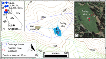
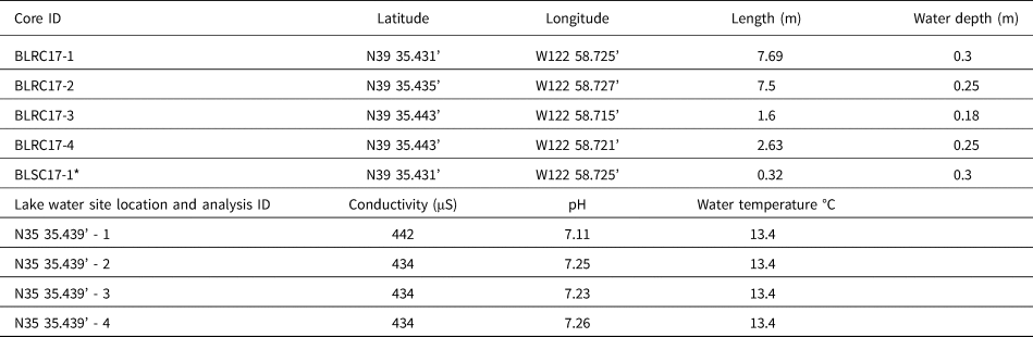
Barley Lake (N39°35.437′, W122°58.732′) is a landslide-formed lake located in Mendocino County (northern California Coast Range), approximately 207 km northwest of San Francisco and 70 km east of the Pacific Ocean (Fig. 1). It is located within the territory of the Witukomnóm subgroup of the Yuki indigenous population (Flaherty and Fredrickson, Reference Flaherty and Fredrickson1981) and lies within the Mendocino National Forest region at an elevation of 1658 m asl. In August 2017, when the coring took place, Barley Lake was ~0.13 km in length and ~0.08 km in width, with a maximum depth of 0.3 m; the drainage basin was ~0.13 km2 (Fig. 1; West, Reference West, Mikkelsen, Hildebrandt and Basgall1993). The average lake water conductivity (15 cm below the surface) at the core site was 436 μS, the average pH was 7.21, and the average temperature was 13.4°C (Table 1). Aquatic macrophytes, mainly water lilies (Nuphar polysepala and Brasenia schreberi), are ubiquitous, covering most of the lake's modern surface (Flaherty and Fredrickson, Reference Flaherty and Fredrickson1981). Its drainage basin is occupied by a variety of conifer and oak species (Pinus jeffreyi, Abies concolor, Libocedrus decurrens, Quercus garryana) (Flaherty and Fredrickson, Reference Flaherty and Fredrickson1981). West (Reference West, Mikkelsen, Hildebrandt and Basgall1993) defines the site's general vegetation type as Coast Range Montane Forest. Some willows (Salix sp.) and a fragmented fringe of sedges grow at the north end of the lake. A well-defined lower limit of trees is evident along the shore. This limit is presently ~2 m above the current lake level and matches the spillover/outlet elevation. The shoreline limit of trees well above the current lake level suggests a time in the recent past when lake levels were sustained higher than at present, perhaps because of a hydrological balance between precipitation and evaporation. There appears to be a few inlets at the northern area of the basin, although none seemed to be active at the time of coring. A small basin, ~0.19 km northwest of Barley Lake and within the same drainage basin (~19 m higher than Barley Lake at 1677 m), would spill into the lake if filled with water. Reconnaissance of this basin evidences recent standing water in the form of mud cracks and a well-defined vegetation line. The main source of water for Barley Lake is likely direct over-water precipitation, precipitation runoff, and possibly groundwater.
(color online) A) Regional map showing Barley Lake (BL) as a red dot and relevant locations as blue dots: NP = North Pacific; CA = California; NV = Nevada; SB = Secret Beach (Rypins et al., Reference Rypins, Reneau, Byrne and Montgomery1989); CleL = Clear Lake (Adam and West, Reference Adam and West1983); FL = Fish Lake (Crawford et al., Reference Crawford, Mensing, Lake and Zimmerman2015); OL = Ogaromtoc Lake (Crawford et al., Reference Crawford, Mensing, Lake and Zimmerman2015); CL = Crater Lake (Mohr et al., Reference Mohr, Whitlock and Skinner2000); ML = Mumbo Lake (Daniels et al., Reference Daniels, Anderson and Whitlock2005); TL = Taylor Lake (Briles et al., Reference Briles, Whitlock, Skinner and Mohr2011); BuL = Bluff Lake (Mohr et al., Reference Mohr, Whitlock and Skinner2000); CrL = Crater Lake (Mohr et al., Reference Mohr, Whitlock and Skinner2000); CamL = Campbell Lake (Briles et al., Reference Briles, Whitlock, Skinner and Mohr2011); B = ODP site 1019 (Barron et al., Reference Barron, Heusser, Herbert and Lyle2003); BoL = Bolan Lake (Briles et al., Reference Briles, Whitlock, Bartlein and Higuera2008); SL = Sanger Lake (Briles et al., Reference Briles, Whitlock, Bartlein and Higuera2008). B) Barley Lake drainage basin and core locations. C) Google Earth view of Barley Lake with core locations (1 = BLRC17–1; 2 = BLRC17–2 & BLSC17–1; 3 = BLRC17–3; 4 = BLRC17–4). (For interpretation of the references to color in this figure legend, the reader is referred to the web version of this article.)

Core data and lake water data.

Note: *same location as BLRC17-1
A long history of archeological research is recorded in the area around Barley Lake (Flaherty and Fredrickson, Reference Flaherty and Fredrickson1981). Archaeological evidence suggests low-density hunter and gatherer populations that established permanent residences near reliable water resources (Flaherty and Fredrickson, Reference Flaherty and Fredrickson1981). Barley Lake is an obvious choice for settlement as it provides both water and game. Although site chronologies are relatively poor, obsidian hydration estimates suggest occupation as early as 7.0 to 4.5 ka in the northern California Coast Range (Meighan and Haynes, Reference Meighan and Haynes1970; Ericson, Reference Ericson, Earle and Ericson1977; Hildebrandt and Hayes, Reference Hildebrandt, Hayes, Mikkelsen, Hildebrandt and Basgall1993; Hildebrandt, Reference Hildebrandt, Jones and Klar2007). We mention this human occupation information because, as noted by Crawford et al. (Reference Crawford, Mensing, Lake and Zimmerman2015) (Fish Lake and Lake Ogaromtoc, California; Fig. 1), human disturbance of the landscape may confound the primary sediment signal as recorded in the region's lake sediments, especially floristic and fire interpretations. For the Barley Lake study presented here, we contend that the human signal was minimal to absent from 12.9 to 8.1 ka. As a result, we argue that our interpretations reflect a natural signal without impactful anthropogenic contributions.
Modern climatology
There are no meteorological records from Barley Lake itself. As a result, we used meteorological data from Potter Valley (34.7 km to the southwest) to infer the lake's general climatology. Annual precipitation averaged about 116 cm/yr at Potter Valley between AD 1937 and 2016 (https://wrcc.dri.edu/), and about 90% of the annual precipitation in the valley occurs during winter. Summer (JJA) precipitation averages 14.8 cm/yr; winter (DJF) precipitation averages 101.5 cm/yr. Consequently, Barley Lake's hydrologic budget is a product of winter precipitation and subsequent summer evaporation. Summer precipitation is considered negligible to the lake's additive hydrologic budget. Groundwater contributions are unknown.
In general, the modern climate of coastal California is Mediterranean, with cool wet winters and hot dry summers. Wetter than average winters in the coastal southwest are attributed to a weakened Pacific subtropical high, which allows storm tracks to shift southward more frequently. When the high-pressure system remains strong, coastal California experiences drier winters, as storms track more frequently across the Pacific Northwest (Peterson, Reference Peterson1989; Schonher and Nicholson, Reference Schonher and Nicholson1989). Superimposed on this unimodal winter climatology is the western U.S. precipitation dipole, located at a 500-year average latitude of 40°N (Redmond and Koch, Reference Redmond and Koch1991; Cayan et al., Reference Cayan, Dettinger, Diaz and Graham1998; Dettinger et al., Reference Dettinger, Cayan, Diaz and Meko1998; Wise, Reference Wise2010, Reference Wise2016; Peng et al., Reference Peng, Yu and Gautam2013). This dipole (dry north/wet south or vice versa) is the predominant hydroclimatic feature of Californian winter climatology. However, it is dynamic (500-year range from 35°N to 44°N) and occasionally absent, thus influencing where the state receives its winter precipitation from year to year (Monier et al., Reference Monier, Gao, Scott, Sokolov and Schlosser2015; Wise, Reference Wise2010, Reference Wise2016). Notably, Barley Lake is located at the 500-year average dipole transition latitude, making it a key site for future Holocene-scale dipole investigations. It is not the intention of this article, however, to examine the regional response of the dipole across the YD to early EH via site-to-site comparisons.
One of the most important types of winter storms to impact coastal California are atmospheric rivers (ARs), particularly the warm Pineapple Express events that produce flooding when delivered as rain instead of snow (Ralph et al., Reference Ralph, Neiman, Wick, Gutman, Dettinger, Cayan and White2006; Dettinger et al., Reference Dettinger, Ralph, Das, Neiman and Cayan2011; Steinschneider et al., Reference Steinschneider, Ho, Williams, Cook and Lall2018). ARs are responsible for transporting vast amounts of water vapor—up to 90% of all tropical/subtropical moisture transported to higher latitudes—into the western United States (Dettinger, Reference Dettinger2011; Dettinger et al., Reference Dettinger, Ralph, Das, Neiman and Cayan2011). ARs account for nearly all the historically large storms and subsequent flooding within the study region (Ralph et al., Reference Ralph, Neiman, Wick, Gutman, Dettinger, Cayan and White2006; Dettinger et al., Reference Dettinger, Ralph, Das, Neiman and Cayan2011; Ralph and Dettinger; Reference Ralph and Dettinger2011). Thus, it is reasonable to conclude that sustained periods of wetter than average paleoclimates are associated with more frequent and/or larger-magnitude ARs (see “Discussion”).
Previous northern California Coast Range paleoclimate research
Briles et al. (Reference Briles, Whitlock, Skinner and Mohr2011) provide a comprehensive summary of late glacial through modern vegetation (i.e., pollen) and fire (i.e., charcoal) reconstructions from northern California and far southern Oregon (Fig. 1). Regional sites discussed by Briles et al. (Reference Briles, Whitlock, Skinner and Mohr2011) that overlap with the Barley Lake record (12.9–8.1 ka) include, in California, Cedar Lake, Bluff Lake, Mumbo Lake, Taylor Lake, Campbell Lake, and Sanger Lake; and, in Oregon, Bolan Lake. Other relevant sites include Clear Lake and Point Reyes Peninsula (Secret Beach) in California and Oregon Cave National Monument and ODP site 1019 (Fig. 1) (Adam and West, Reference Adam and West1983; Rypins et al., Reference Rypins, Reneau, Byrne and Montgomery1989; West, Reference West, Mikkelsen, Hildebrandt and Basgall1993; Heusser, Reference Heusser1998; Mohr et al., Reference Mohr, Whitlock and Skinner2000; Barron et al., Reference Barron, Heusser, Herbert and Lyle2003; Daniels et al., Reference Daniels, Anderson and Whitlock2005; Vacco et al., Reference Vacco, Clark, Mix, Cheng and Edwards2005; Briles et al., Reference Briles, Whitlock, Bartlein and Higuera2008; Ersek et al., Reference Ersek, Clark, Mix, Cheng and Edwards2012; Anderson et al., Reference Anderson, Wahl and Bhattacharya2020). In general, the late glacial (<15–12.9 ka) terrestrial climate was cooler and wetter than the modern period but warmer and wetter than the full glacial conditions. Forests were more open, the understory was less dense, and drainage basins were more exposed to weathering and erosion (Mohr et al., Reference Mohr, Whitlock and Skinner2000; Daniels et al., Reference Daniels, Anderson and Whitlock2005; Briles et al., Reference Briles, Whitlock, Skinner and Mohr2011). How seasonal (perennial?) snowpack changed across the YD to EH is unknown; however, a cooler YD climate might suggest that occasional perennial snowpack was more common, thus influencing the drainage basin's response to runoff at this time. Pollen evidence for a wetter YD (12.9–11.7 ka [chronozone, cf. Rasmussen et al., Reference Rasmussen, Andersen, Svensson, Steffensen, Vinther, Clausen and Siggaard-Andersen2006]) is site-dependent and seems to reflect variations in substrate type per site and its sensitivity to climate change; pollen evidence for temperature change during the YD is also site-dependent and not well expressed equally by the pollen records (Briles et al. Reference Briles, Whitlock, Skinner and Mohr2011). However, the longest fire return episode intervals occur during the YD, suggesting wetter than modern conditions (Briles et al., Reference Briles, Whitlock, Skinner and Mohr2011). In summary, all the regional sites above indicate a transition from a wetter/colder late glacial to a warmer/drier EH with a site- or proxy-specific YD signal.
METHODS
The collection of four Russian cores and one surface gravity core from Barley Lake took place in August 2017 (Fig. 1, Table 1). Overlapping cores BLRC17-1 (7.69 m length) and BLRC17-2 (7.5 m length) were collected approximately 2 m apart using a Russian corer in 0.3 and 0.25 m water depth, respectively (Table 1). The section of core BLRC17-2 (core 2) spanning 750 to 474 cm (12.9–8.1 ka cal yr BP) is the focus of this article. A Russian core was selected for this project because it provided rapid, self-contained 1-m sediment core sections. It is especially effective in organic-rich sediments. Cores 1 and 2 were vertically offset to capture potential gaps caused by the coring process. All cores were opened, described, photographed in the field, and subsequently wrapped in plastic wrap and PVC pipe for transport to California State University, Fullerton (CSUF), where they were stored at 4°C. The two near-shore cores (BLRC17-3 and BLRC17-4 [Table 1]) are not discussed here, as they did not extend vertically in time to the period of study.
BLRC17-1 and core 2 were subsampled at 1-cm contiguous intervals to determine magnetic susceptibility (x 10-7 m3 kg-1), percent water content, and loss on ignition at 550°C (percent total organic matter [TOM]) and 950°C (percent total carbonate), following standard CSUF laboratory protocols (Dean, Reference Dean1974; Kirby et al., Reference Kirby, Lund, Anderson and Bird2007). Grain size was measured on core 2 at every other centimeter from 486 to 658 cm and at every centimeter from 660 to 749 cm using a Malvern Mastersizer 2000 laser diffraction grain-size analyzer coupled to a Hydro 2000G. All grain samples were pretreated with 30 mL of ≥30% H2O2 to remove organics, 10 mL of 1 N HCl to remove carbonates, and 10 mL of 1 N NaOH to remove biogenic silica. A silica carbide polishing powder standard was run twice at the beginning of each day, once every 10 samples, and once at the end of every day to evaluate the equipment's analytical stability over time (n = 2923, avg. = 13.10 μm, SD = 0.08 μm). All data are reported as volume percent and divided into 10 grain-size intervals according to the Wentworth scale (Wentworth, Reference Wentworth1922) as well as d0.5 (0.5 = mean), percent clay (0.02–3.9 μm), percent silt (3.91–62.49 μm), percent sand (62.5–2000 μm), very fine sand (VFS = 62.5–124.99 μm), fine sand (FS = 125–249.99 μm), medium sand (MS = 250–499.99 μm), coarse sand (CS = 500–1000 μm), and very coarse sand (VCS = 1000.01–2000 μm). The percent MS to VCS and total percent clay data were standardized by subtracting the mean of the distribution (as calculated between 690 and 486 cm [= EH]) from each percent sand value and dividing the subsequent value by the standard deviation (derived for the interval 690–486 cm). The standardization process created a mean of zero, with deviations from the mean in units of standard deviation.
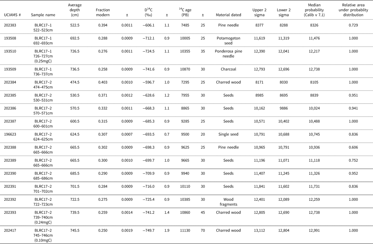
For the interval 750–474 cm (12.9–8.1 ka), four samples of discrete organic material from BLRC17-1 and 12 samples from core 2 were isolated and photographed after a >125 μm wet sieving. In total, 16 AMS 14C dates were measured at the Irvine Keck Carbon Cycle AMS Laboratory, University of California. All samples were pretreated using a standard acid–base–acid method.
RESULTS
BLRC17-1 and core 2 show a similar stratigraphy (see percent TOM below). In general, core 2 (750–474 cm [12.9–8.1 ka cal yr BP]) is characterized by variegated brown, organic-rich sediment with occasional faint darker brown to dark red-black laminae (Fig. 2). A change to interbedded light gray and dark brown laminations appears at 712–706 cm and 696–692 cm. The base of core 2, from 750 to 734.5 cm, is characterized as gray to gray-black with laminae and visibly coarser components. The act of coring ended at 750 cm for core 2 because of increased friction associated with the dense basal sediments. BLRC17-1, however, extended to 768 cm; this additional 18 cm of sediment in core 1 is visually similar to the sediment at the bottom of core 2. We suspect there remains mud deeper than 768 cm that would require mechanical coring to obtain. In other words, the basal coring limitations and associated ages are not considered correlative to the lake's formation. Finally, occasional macroorganics were observed throughout the core, such as pine needles and visually apparent charcoal pieces.
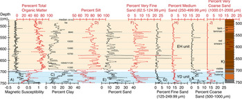
Core BLRC17–2 data. A) Magnetic susceptibility and ages (cal BP). B) Percent total organic matter (TOM). C) Percent clay. D) Percent silt. E) Percent total sand. F) Percent very fine sand. G) Percent fine sand. H) Percent medium sand. I) Percent coarse sand. J) Percent very coarse sand. K) Lithostratigraphic column based on visual inspection of core. Colors are subjective lake sediment color; the light blue shaded area highlights the Younger Dryas (YD) sediment unit; the light orange shaded area highlights the Early Holocene (EH) sediment unit; the transition sediment unit is unshaded. (For interpretation of the references to color in this figure legend, the reader is referred to the web version of this article.)

For the interval 750–474 cm, core 2 magnetic susceptibility (MagS) values average -0.08 (± 0.21) x 10-7 m3 kg-1, with a maximum of 1.05 and a minimum of -0.48 (Fig. 2). MagS values are highest and positive at the base of the core (750 cm), with a decreasing trend until 736 cm. From 736 to 703 cm, the values are positive and stable. An abrupt shift occurs at 703 cm to generally negative values, with no significant trends through to 474 cm. There is a general decrease in the amplitude of MagS variability from 550 to 474 cm.
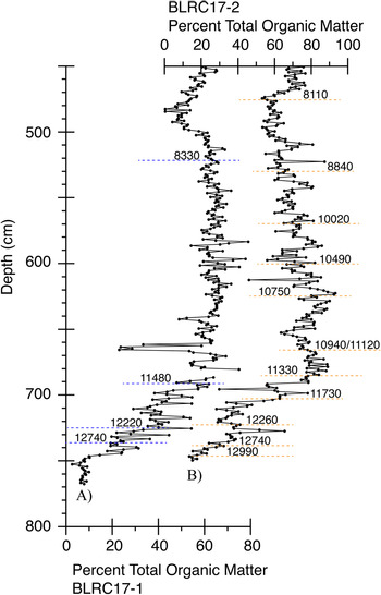
TOM values in core 2 average 64.5% (± 17.2%), with a maximum of 93.1% and a minimum of 13.4% (Fig. 2). Values are lowest at the base of the core (750 cm), with an increasing trend until 690 cm. From 690 to 474 cm, the values are generally high (>50%) but generally decrease. A comparison of the percent TOM between BLRC17-1 and core 2 shows similar changes with depth (Fig. 3). Dates are also shown in Figure 3, indicating that both cores capture the same sediment units in time. Therefore, we focus on the master core, BLRC17-2 (core 2), because it contains the most ages for developing a robust age model (see below). Loss on ignition at 950°C analysis did not detect any carbonates in the core sediments.
(color online) A comparison of percent TOM and age (ka) between adjacent and overlapping cores A) BLRC17-1 and B) BLRC17-2 to demonstrate the consistency in age depth and percent TOM.

The average grain size (d0.5) in core 2 is 15.8 μm (silt-dominated) (± 7.64 μm), with a maximum of 51 μm and a minimum of 5.1 μm (Fig. 2). Clay averages 11.5% (± 7.0%), with a maximum of 35.1% and a minimum of 1.4%. Silt averages 76.2% (± 9.0%), with a maximum of 94.6% and a minimum of 50.6%. Sand averages 12.2% (± 6.8%), with a maximum of 41.2% and a minimum of 2.2%. From 750 to 734 cm, the sediment is characterized as sandy silt. Sand decreases abruptly at 734 cm as the percent clay begins to increase, reaching a peak in percent clay at 690 cm. From 734 to 690 cm, the sediment is characterized as clayey silt. From 690 to 486 cm, the sediment alternates between clayey silt and sandy silt; however, silt averages 80% from 690 to 486 cm, indicating a silt-dominated sediment size. There is a notable shift to a higher percent clay content at 578–486 cm. The percent sand is uniformly low from 700 to 486 cm but with notable variability. The standardized percent MS to VCS and the total percent clay (as calculated between 690 and 486 cm [= EH]) are discussed vs. time below.
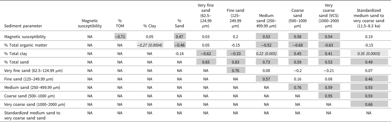
Critical to assessing the interpretative value of each sediment measurement is their respective interrelationships (i.e., correlations). As a result, we conducted a simple correlation analysis between key sedimentological parameters (Table 2). The details of these correlations relative to their proxy interpretations are presented in the “Discussion” section.
Sediment property correlation coefficients (r-value).

Note: *dark gray highlighted significant at p < 0.0001
Note: *light gray highlighted significant at p < 0.05
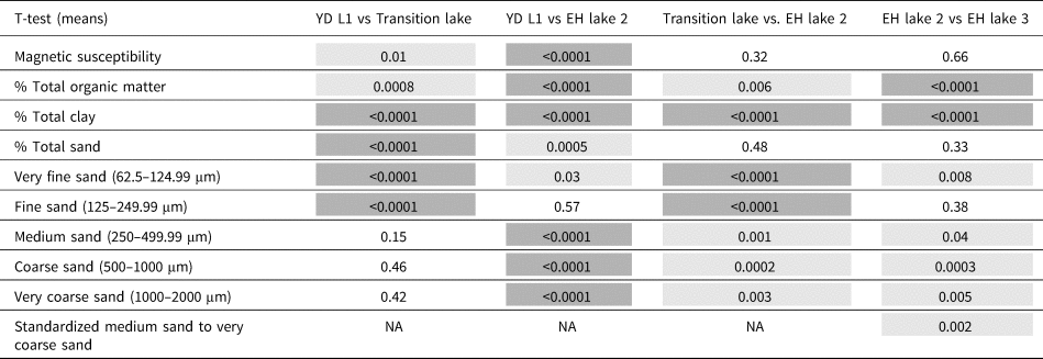
We also examined the difference in the sediment data mean values using Student's t-test for unpaired data with unequal variance between four visually determined sediment units (Table 3). Although initially based on a subjective visual assessment, our statistical analysis shows that our visual assessment was reasonable and statistically objective. The four statistically distinct sediment units are the YD unit, the Transition unit, EH unit 1, and EH unit 2. This statistical measure of sediment unit similarities and differences provides the foundation of our lake state model (see “Discussion”).
Chronostratigraphic unit sediment data t-test probabilities.

Note: *dark gray highlighted significant at p < 0.0001
Note: *light gray highlighted significant at p < 0.05
Note: EH = Early Holocene, YD = Younger Dryas
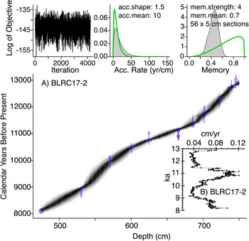
Finally, an age model was created using the 12 radiocarbon dates from BLRC17-2 entered into the Bacon (version 2.2, IntCal13) age-modeling software (Blaauw and Christen, Reference Blaauw and Christen2011) (Fig. 4, Table 4). Sedimentation rates average 0.06 cm/yr (± 0.02), or 17.3 yr/cm (± 6.3), with a maximum of 0.12 cm/yr (or 8.3 yr/cm) and a minimum of 0.03 cm/yr (or 31 yr/cm) (Fig. 4). As a result, we conclude that our new sediment record captures multidecadal information, with appropriate age control for future site-to-site comparisons (Zimmerman and Wahl, Reference Zimmerman and Wahl2020).
(color online) A) BLRC17-2 age-depth plot using the Bacon (version 2.2, IntCal13) age-modeling software (Blaauw and Christen, Reference Blaauw and Christen2011). B) Sedimentation-rate plot (cm/yr) based on the age model.

Radiocarbon data for cores BLRC17-1 and BLRC17-2.

Note: All samples were treated with acid-base-acid (1N HCl and 1N NaOH, 75°C) prior to combustion. PB = pre-bomb.
DISCUSSION
Proxy interpretations
MagS and TOM
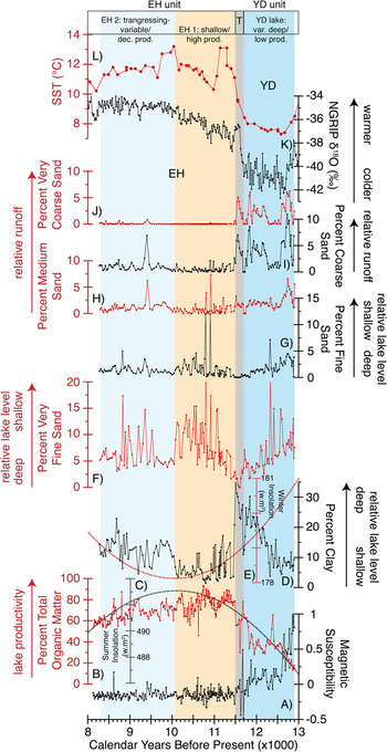
MagS in lake sediments is often interpreted as an indicator of magnetic-mineral runoff from a lake's drainage basin (Thompson et al., Reference Thompson, Battarbee, O'Sullivan and Oldfield1975; Dearing, Reference Dearing, Maher and Thompson1999; Brown et al., Reference Brown, Bierman, Lini, Davis and Southon2002; Kirby et al., Reference Kirby, Poulsen, Lund, Patterson, Reidy and Hammond2004, Reference Kirby, Lund, Anderson and Bird2007). However, in the presence of high organic content and a reducing lacustrine sedimentary environment, magnetic minerals may dissolve, producing low to negative values (Karlin and Levi, Reference Karlin and Levi1983; Hilton and Lishman, Reference Hilton and Lishman1985; Canfield and Berner, Reference Canfield and Berner1987; Anderson and Rippey, Reference Anderson and Rippey1988; Tarduno, Reference Tarduno1995; Reynolds et al., Reference Reynolds, Rosenbaum, van Metre, Tuttle, Callender and Goldin1999). In Barley Lake, percent TOM is negatively correlated with MagS (r = -0.71, p < 0.0001) for the breadth of the core, suggesting that intervals of higher percent TOM either dilute or enhance the reduction and dissolution of the MagS signal (Fig. 5, Table 2).
Core BLRC17-2 sediment data vs. potential climate forcings. From bottom to top: A) Magnetic susceptibility. B) Percent TOM. C) JJA summer insolation (W.m-2) at 39°N. D) Percent clay. E) DJF winter insolation (W.m-2) at 39°N. F) Percent very fine sand. G) Percent fine sand. H) Percent medium sand. I) Percent coarse sand. J) Percent very coarse sand. K) North Greenland Ice Core Project δ18O (‰) (Andersen et al., Reference Andersen, Svensson, Johnsen, Rasmussen, Bigler, Röthlisberger, Ruth, Siggaard-Andersen, Steffensen and Dahl-Jensen2006; Rasmussen et al., Reference Rasmussen, Andersen, Svensson, Steffensen, Vinther, Clausen and Siggaard-Andersen2006). L) ODP site 1019 SST (Barron et al., Reference Barron, Heusser, Herbert and Lyle2003). Shading represents the relative lake level (dark blue = deepest; light beige = shallowest; gray = transition zone from the YD to the EH lakes); proxy interpretations are shown by arrow direction and labels on the y-axes, respectively. (For interpretation of the references to color in this figure legend, the reader is referred to the web version of this article.)

For a closer look at these two end-member interpretations (i.e., dilution vs. dissolution), we examined the correlation between percent TOM and MagS for the YD unit and the EH unit independently (Fig. 2). Our rationale for this YD to EH separation is that MagS values are variable and generally greater than zero during the YD unit. Conversely, they are stable and uniformly less than zero in the EH unit. In other words, the YD unit records measurable, likely ferrimagnetic mineral, input, while the EH unit is essentially absent of magnetic minerals, as reflected by its diamagnetic signal (i.e., typical of organic-rich sediments) (Gale and Hoare, Reference Gale and Hoare1991).
For the YD unit (750–699 cm), a very strong negative correlation between percent TOM and MagS is evident (r = -0.81, p < 0.001) (Fig. 2). A positive correlation is also evident between MagS and the all the sand-size fractions in the YD unit (VFS r = 0.30, FS r = 0.45, MS r = 0.53, CS r = 0.36, VCS r = 0.29, p < 0.05). Based on these relationships, we conclude that the MagS signal in the YD unit reflects the combined processes of (1) a higher influx of sand-sized (VFS and VCS) ferrimagnetic minerals, perhaps related to less impeded runoff from a drainage basin and characterized by a more open forest and less well-developed soils (Mohr et al., Reference Mohr, Whitlock and Skinner2000; Daniels et al., Reference Daniels, Anderson and Whitlock2005; Briles et al., Reference Briles, Whitlock, Skinner and Mohr2011); and (2) the dissolution and/or dilution of magnetic minerals during intervals in the YD unit, characterized by a higher percent TOM (Figs. 2 and 5) (Karlin and Levi, Reference Karlin and Levi1983; Hilton and Lishman, Reference Hilton and Lishman1985; Canfield and Berner, Reference Canfield and Berner1987; Anderson and Rippey, Reference Anderson and Rippey1988; Tarduno, Reference Tarduno1995; Reynolds et al., Reference Reynolds, Rosenbaum, van Metre, Tuttle, Callender and Goldin1999). Notably, the YD interval contains the highest percent CS and VCS, which should be more resistant to chemical dissolution, thus maintaining MagS values generally greater than zero, even during periods of a higher percent TOM (Figs. 2 and 5).
For the EH unit (690–474 cm, not including the Transition unit [691–698 cm]), no significant relationship is evident between percent TOM and MagS (r = -0.03). Importantly, the EH unit MagS values are stable and uniformly less than zero, indicating a strong diamagnetic signal (Gale and Hoare, Reference Gale and Hoare1991), which is typical for organic-rich lake sediments. The most conservative explanation for this diamagnetic signal is the abundance of organic matter in the EH unit. A wealth of literature shows that magnetic minerals experience chemical dissolution in organic-rich reducing sedimentary environments (Karlin and Levi, Reference Karlin and Levi1983; Hilton and Lishman, Reference Hilton and Lishman1985; Anderson and Rippey, Reference Anderson and Rippey1988; Tarduno, Reference Tarduno1995; Reynolds et al., Reference Reynolds, Rosenbaum, van Metre, Tuttle, Callender and Goldin1999). Therefore, the lack of a MagS signature in the EH unit is interpreted to reflect dissolution in the presence of high percent TOM (Figs. 2 and 5). However, it is worth noting that a weak positive correlation between the coarsest sands (CS and VCS) and MagS (r = 0.25, r = 0.20, p < 0.05), or those sizes most resistant to chemical alteration, is observed in the EH unit. This weak positive correlation between MagS and CS/VCS may indicate a weak and subordinate role for dilution of percent TOM by CS/VCS magnetic minerals in the EH unit.
In all, the interpretative value of the MagS data as a sediment process proxy is constrained in our discussion of the YD unit, where MagS values exceed zero and are interpreted to reflect more runoff of sand-sized magnetic minerals. For the EH unit, the absence of a positive MagS signal is interpreted simply as additional support that the EH unit is characterized by higher productivity than the YD unit. In other words, the EH unit MagS data are irrelevant to the interpretation of the EH lakes discussed below.
In lake sediments, TOM often reflects a lake's productivity (Qiu et al., Reference Qiu, Williams, Gvorzdkov, Karabanov and Shimaraeva1993; Hodell and Scheslske, Reference Hodell and Schelske1998; Kirby et al., Reference Kirby, Lund, Anderson and Bird2007; Kołaczek et al., Reference Kołaczek, Mirosław-Grabowska, Karpińska-Kołaczek and Stachowicz-Rybka2015; MacDonald et al., Reference MacDonald, Moser, Bloom, Potito, Porinchu, Holmquist, Hughes and Kremenetski2016). However, percent TOM in lake sediments is influenced by both autochthonous and allochthonous sources. And without the benefit of C:N data, it is difficult to discern their relative contributions (Meyers and Ishiwatari, Reference Meyers and Ishiwatari1993). For Barley Lake, we suggest that allochthonous organic matter contributions are minor relative to the lake's autochthonous organic productivity. This assumption is based on the modern distribution of ubiquitous submergent, emergent, and floating macrophytes, such as N. polysepala and B. schreberi, which dominate the lake environment (Flaherty and Fredrickson, Reference Flaherty and Fredrickson1981). Of course, it is possible that the contribution of allochthonous organic matter was more significant during the YD unit, when seasonal ice cover and assumed cooler lake water temperatures impeded autochthonous organic productivity. Inferred greater runoff during the YD (see “Grain size” below and the MagS interpretation above) may also have generated a concomitant increase in the flux of terrestrial organic detritus into the lake (Kirby et al., Reference Kirby, Zimmerman, Patterson and Rivera2012). However, without additional data, we defer to the most conservative interpretation that a higher percent TOM reflects higher lake productivity and vice versa, especially in the organic-rich EH unit (avg. EH unit percent TOM = 71.5 ± 9.5% vs. YD unit percent TOM = 36.1 ± 13.5%) (Fig. 5).
Grain size
Changes in lake sediment grain sizes are related to lake depth/lake level, distance from the shoreline, and grain size/energy dynamics associated with runoff from the drainage basin (Anderson, Reference Anderson1977; Davis and Ford, Reference Davis and Ford1982; Hilton, Reference Hilton1985; Blais and Kalff, Reference Blais and Kalff1995; Dearing, Reference Dearing1997; Kirby et al., Reference Kirby, Lund, Patterson, Anderson, Bird, Ivanovici, Monarrez and Nielsen2010, Reference Kirby, Knell, Anderson, Lachniet, Palermo, Eeg, Lucero, Murrieta, Arevalo and Silveira2015, Reference Kirby, Heusser, Scholz, Ramezan, Anderson, Markle and Rhodes2018; Bird et al., Reference Bird, Lei, Perello, Polissar, Yao, Finney, Bain, Pompeani and Thompson2017; Pribyl and Shuman, Reference Pribyl and Shuman2017; Shuman and Serravezza, Reference Shuman and Serravezza2017). In general, finer grain sizes are deposited in lower-energy environments, such as a lake's depocenter or its most distal point from the shoreline. Conversely, coarser sediments are associated with the higher-energy shoreline environments, where the finer sediment is easily eroded and focused into the deeper water (Lehman, Reference Lehman1975; Håkanson and Jansson, Reference Håkanson and Jansson1983; Dearing, Reference Dearing, Smith, Appleby, Battarbee, Dearing, Flower, Haworth, Oldfield and O'Sullivan1991; Kirby et al., Reference Kirby, Knell, Anderson, Lachniet, Palermo, Eeg, Lucero, Murrieta, Arevalo and Silveira2015; Bird et al., Reference Bird, Lei, Perello, Polissar, Yao, Finney, Bain, Pompeani and Thompson2017; Pribyl and Shuman, Reference Pribyl and Shuman2017). The energy change from a depositional to an erosional environment is referred to as the “mud-depth boundary” (i.e., mud-line depth) (Stanley and Wear, Reference Stanley and Wear1978). As lake level rises, the mud-depth boundary migrates landward and vice versa as lake level falls. The result of the mud-depth boundary migration is often reflected in sediment grain-size distributions. As a result, the measurement of grain-size distributions in a sediment core extracted from a lake—especially a small, hydrologically sensitive lake such as Barley Lake—should record this migration. However, superimposed on this mud-depth boundary/shoreline migration concept are changes in the flux of coarser grain-sized sediments in response to enhanced runoff during storms and/or wetter climate states that may or may not co-occur with lake-level changes. To evaluate the mud-depth boundary migration vs. the runoff hypotheses, we examined the various grain-size relationships in core 2 (Table 2). Notably, core 2 was extracted from Barley Lake's central basin and assumed depocenter, thus representing an ideal location for potentially capturing both signals.
We focus our discussion on the end-member grain sizes of clay (avg. 11.5 ± 7%) and sand (avg. 12.3 ± 6.9%) rather than on the dominant and ubiquitous silt component (avg. = 76.1 ± 9.1%). Our rationale for this is that small changes in the end-member sizes should capture more subtle energy dynamics, such as those associated with mud-depth boundary migration and runoff not captured (or as apparent) in the dominant silt fraction.
To test the mud-depth boundary hypothesis, we examined the correlations between clay and sand (Table 2). We assumed that higher percent clay represents a lower-energy environment and thus a deeper lake. As clay content rises (the mud-depth boundary migrates landward), a corresponding decrease in sand content should be evident. Comparing clay and sand, we observed a statistically significant negative correlation between clay and VFS/FS (Table 2). As a result, we interpreted the changes in clay and VFS/FS as lake-level indicators (Fig. 5). As lake level rises, the clay content increases, and VFS/FS decrease as the mud-depth boundary migrates landward. The opposite occurs as lake level falls.
To evaluate the runoff hypothesis, we examined further the relationship between clay and sand. Notably, a statistically significant positive relationship occurs between clay and MS/VCS (Table 2), suggesting that the coarsest sand reflects a process unrelated to the mud-depth boundary migration hypothesis. In general, the transportation of sand into a lake basin, particularly the depocenter, requires high-energy dynamics, such as enhanced precipitation over the drainage basin and its associated influence on runoff. This sand-runoff relationship (higher percent sand = greater runoff) is observed both in modern process studies and in paleostudies in California (Inman and Jenkins, Reference Inman and Jenkins1999; Farnsworth and Milliman, Reference Farnsworth and Milliman2003; Romans et al., Reference Romans, Normark, McGann, Covault and Graham2009; Warrick and Mertes, Reference Warrick and Mertes2009; Covault et al., Reference Covault, Romans, Fildani, McGann and Graham2010; Kirby et al., Reference Kirby, Lund, Patterson, Anderson, Bird, Ivanovici, Monarrez and Nielsen2010, Reference Kirby, Feakins, Hiner, Fantozzi, Zimmerman, Dingemans and Mensing2014, Reference Kirby, Heusser, Scholz, Ramezan, Anderson, Markle and Rhodes2018, Reference Kirby, Patterson, Lachniet, Noblet, Anderson, Nichols and Avila2019; Xu et al., Reference Xu, Swarzenski, Noble and Li2010; Warrick and Barnard, Reference Warrick and Barnard2012; Gray et al., Reference Gray, Warrick, Pasternack, Watson and Goñi2014; Warrick et al., Reference Warrick, Melack and Goodridge2015; Hiner et al., Reference Hiner, Kirby, Bonuso, Patterson, Palermo and Silveira2016). Based on the statistically significant positive relationship between clay and MS/VCS, we interpreted the coarsest sand sizes (MS, CS, VCS) as reflecting variations in runoff from the lake's drainage basin associated with either discrete precipitation events or wetter than average periods of past climate (Fig. 5). Because the sand in core 2 was not observed as discrete layers, and because 1 cm of sediment integrated a multidecadal signal, we favor the latter interpretation that a higher percent MS, CS, and VCS records multidecadal periods of wetter than average past climate. To assess runoff variability, we standardized the MS, CS, and VCS data and focused only on the EH (690–486 cm, 11.5–8.1 ka). This avoided the influence on runoff caused by large changes in drainage basin vegetation during the late glacial vs. the EH, which may unnecessarily obfuscate the runoff interpretation (Figs. 5 and 6) (Briles et al., Reference Briles, Whitlock, Skinner and Mohr2011).
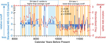
Inferred early Holocene runoff and relative lake level for Barley Lake. Left axis (blue bars) = BLRC17-2 standardized medium to very coarse sand. Right axis (red line plot with dots) = BLRC17-2 standardized clay data. Colored bars represent two or more positive or negative adjacent standardized MS to VCS sand values: blue = higher than average runoff, orange = lower than average runoff; purple bars represent two extreme values exceeding four standard deviations positive sand. (For interpretation of the references to color in this figure legend, the reader is referred to the web version of this article.)

In summary, changes in percent clay and VFS/FS are interpreted to reflect lake level/ mud-depth boundary migration (i.e., higher clay/lower VFS/FS = deeper lake and vice versa), whereas changes in percent MS/VCS are interpreted to reflect variations in precipitation-related runoff from the lake's drainage basin (i.e., higher percent MS/VCS = greater runoff and vice versa) (Figs. 5 and 6). Notably, the clay and VFS/FS lake-level proxy data show a positive and statistically significant correlation to the MS/VCS runoff proxy data (r = 0.35, p < 0.0003) (Fig. 7). In other words, as lake level rises (higher clay, lower VFS/FS), runoff increases (higher MS/VCS). Because these two sediment-based processes are acting on different timescales (i.e., lake levels rise and fall at different rates than the deposition of discrete runoff events), this positive correlation adds confidence to the veracity of our interpretations.
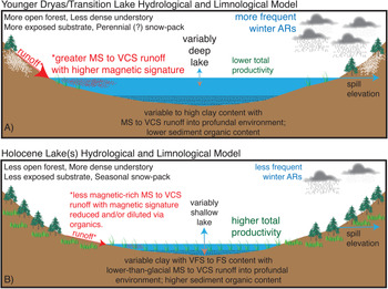
Simple lake hydrological and limnological models. A) YD/ Transition lake model. B) EH lake(s) model. VFS = very fine sand; FS = fine sand; MS = medium sand; CS = coarse sand; VCS = very coarse sand; ARs = atmospheric rivers; white-dotted pattern represents seasonal and perennial(?) snowpack during the late glacial; red-dotted pattern represents MS to VCS runoff. (For interpretation of the references to color in this figure legend, the reader is referred to the web version of this article.)

YD–EH limnological and hydrological history of Barley Lake
Based on a simple statistical comparison of the various sediment data, we inferred four different states at Barley Lake spanning 12.9–8.1 ka (Table 3). These include (1) YD lake (12.9–11.7 ka), (2) Transition lake (11.7–11.5 ka), (3) EH lake 1 (11.5–10.1 ka), and (4) EH lake 2 (10.1–8.1 ka).
YD lake (12.9–11.7 ka) and Transition lake (11.7–11.5 ka)
The YD lake is interpreted as a variably deep lake with lower productivity and generally greater runoff (Fig. 5). In the early YD, the clay content was low but was compensated by a much higher sand content in all size classes. In other words, runoff was greatly enhanced in the early YD, diluting the clay in an otherwise deep lake. This likely reflects a drainage basin characterized by a more open forest, a less dense understory, less well-developed soils, and a drainage basin more exposed to weathering and erosion (Mohr et al., Reference Mohr, Whitlock and Skinner2000; Daniels et al., Reference Daniels, Anderson and Whitlock2005; Briles et al., Reference Briles, Whitlock, Skinner and Mohr2011). As the drainage basin evolved, unimpeded runoff diminished, clay content rose, and lake productivity increased. Despite the evolution of the drainage basin, the contribution of the coarsest sands (CS and VCS) varied but remained much higher than anything observed in the EH, suggesting that runoff during the YD was more extreme, or generally less impeded, than in the EH (Fig. 5).
The Transition lake is very similar (but statistically distinct; Table 3) to the YD lake, perhaps slightly deeper, with low productivity and still greater runoff than the two EH lakes (Fig. 5). Our rationale for separating the two late-glacial lakes is based on our use of the YD as a chronostratigraphic unit (Mangerud, Reference Mangerud2020). We have a radiocarbon date at 11.73 ka (Table 4), delimiting the younger boundary of the YD's chronostratigraphic definition. Therefore, we decided to separate the YD lake from the EH lakes by a Transition lake. Of course, the YD may be temporally variable from site to site. If we accept this temporal variability as an alternative interpretation, the YD lake extends to 11.5 ka, and the transition to the EH lakes occurs in less than ~30 years (Fig. 5). Figure 7A illustrates a simple lake hydrological and limnological model for the YD and Transition lakes.
EH lake 1 (11.5–10.1 ka) and EH lake 2 (10.1–8.1 ka)
A dramatic shift in the limnological and hydrological conditions at Barley Lake characterizes the YD and Transition lakes from the two EH lakes (Fig. 5). In general, the EH lakes are characterized as shallow, highly productive, and with lower runoff. The <30-year period separating them from the Transition lake indicates a rapid reorganization of the limnological and hydrological system at the study site. However, a close look at the EH lake sediment data reveals two different EH lakes (Fig. 5).
EH lake 1 is interpreted as a shallow, highly productive lake with diminished runoff, and EH lake 2 is interpreted as a transgressive (but still shallow), less productive lake with an increase in runoff (Fig. 5 and Table 3). Evidence for this change includes a statistically significant increase in percent clay, VFS, MS, CS, and VCS and a significant decrease in percent TOM between EH lake 1 and EH lake 2 (Fig. 5). According to our age model, this transition between the two EH lakes occurs in <20 years. Figure 7B illustrates a simple lake hydrological and limnological model for the EH lakes.
EH runoff history
To evaluate the history of winter precipitation–associated runoff, we standardized the combined percent MS, CS, and VCS for the EH (11.5–8.3 ka), following the same California-based paleostudy protocols used for Lake Elsinore (Kirby et al., Reference Kirby, Lund, Patterson, Anderson, Bird, Ivanovici, Monarrez and Nielsen2010, Reference Kirby, Feakins, Bonuso, Fantozzi and Hiner2013, Reference Kirby, Heusser, Scholz, Ramezan, Anderson, Markle and Rhodes2018), Zaca Lake (Kirby et al., Reference Kirby, Feakins, Hiner, Fantozzi, Zimmerman, Dingemans and Mensing2014), and Abbott Lake (Hiner et al., Reference Hiner, Kirby, Bonuso, Patterson, Palermo and Silveira2016) (Fig. 6). We did not include the YD or the Transition lake in this assessment to avoid combining processes associated with the two different climate states—YD vs. EH—and the documented differences in YD vs. EH forest, its understory density, and the drainage basin's susceptibility to less impeded runoff during the YD (Fig. 7) (Mohr et al., Reference Mohr, Whitlock and Skinner2000; Daniels et al., Reference Daniels, Anderson and Whitlock2005; Briles et al., Reference Briles, Whitlock, Skinner and Mohr2011). We binned by color (blue = above-average runoff, orange = below-average runoff) two or more positive or negative adjacent standardized values (Fig. 6). Because ARs account for the most significant winter precipitation in the region, we also suggest that these changes in runoff record changes in the frequency and/or magnitude of landfalling ARs (Ralph et al., Reference Ralph, Neiman, Wick, Gutman, Dettinger, Cayan and White2006; Dettinger et al., Reference Dettinger, Ralph, Das, Neiman and Cayan2011; Ralph and Dettinger, Reference Ralph and Dettinger2011). Notably, ARs occur during both wet and dry climate states, so changes in runoff should not be overinterpreted as necessarily a wetter than average winter climate. However, the fact that each grain-size sample integrates a multidecadal signal, as opposed to a discrete sand layer, suggests that the above-average standardized sand most likely reflects general changes in the frequency and/or magnitude of past ARs and thus sustained multidecadal periods of a wetter than average climate (and vice versa for below-average sand). Using this AR/winter wetness interpretation, a notable period of a lower than average runoff occurs between 11.5 and 9.9 ka cal yr BP, followed by a period of a higher than average runoff from 9.9 to 8.3 ka cal yr BP (Fig. 6). The latter period reveals a more variable runoff as well.
We compared this MS/VCS runoff proxy to the clay and VFS/FS lake-level proxy (Fig. 6). This revealed a positive and statistically significant correlation (r = 0.35, p < 0.0003) (Fig. 6). In other words, as lake level rises (higher clay, lower VFS/FS), runoff increases (higher MS/VCS). This correlation fits with the interpretation that, in general, wetter climate states are associated with more runoff and thus higher lake levels. The match is not perfect of course because the two proxies are likely recording temporally different dynamics. For example, Kirby et al. (Reference Kirby, Lund, Patterson, Anderson, Bird, Ivanovici, Monarrez and Nielsen2010) developed a lake-level grain-size model for Lake Elsinore showing that a drop in lake level occurs over decades, whereas a lake-filling event can occur during a single large storm or wetter than average winter. Based on this model, the sedimentary imprint of a migrating mud-depth boundary should require more time for sediment deposition, accumulation, and preservation than would a singularly produced AR runoff event. As a result, the clay lake-level interpretation does not match the MS/VCS runoff interpretation one-to-one (Fig. 6).
Forcings
To evaluate potential climate forcings, we compared the Barley Lake data to the NGRIP stable oxygen isotope record and the northeast Pacific ODP site 1019 (41.682°N, W124.930°W) alkenone SST reconstruction (Barron et al., Reference Barron, Heusser, Herbert and Lyle2003; Andersen et al., Reference Andersen, Svensson, Johnsen, Rasmussen, Bigler, Röthlisberger, Ruth, Siggaard-Andersen, Steffensen and Dahl-Jensen2006; Rasmussen et al., Reference Rasmussen, Andersen, Svensson, Steffensen, Vinther, Clausen and Siggaard-Andersen2006) (Fig. 5). Our rationale for using the Barron et al. (Reference Barron, Heusser, Herbert and Lyle2003) record is based on its adequate age control, sample resolution (avg. = ~104 years per SST sample), and proximity to the study site (~290 km northwest of Barley Lake). Together, the NGRIP and ODP 1019 SST data are interpreted as indicators of changing ocean-atmosphere dynamics in the Northern Hemisphere. We also compared our data to summer (JJA) and winter (DJF) insolation at 39°N latitude as indicators of summer evaporation and winter temperature, respectively (Laskar et al., Reference Laskar, Robutel, Joutel, Gastineau, Correia and Levrard2004) (Fig. 5).
Our comparison suggests that Barley Lake is capturing the timing of the major atmospheric and oceanic temperature signals associated with the transition from the YD to the EH (Fig. 5). This hemispheric coupling is likely manifested through the changing Northern Hemisphere atmospheric and SST gradients, their modulation of the mean position and strength of the North Pacific high- and Aleutian low-pressure systems, and their combined influence on the average latitude of winter storm tracks across the western United States (Oster et al., Reference Oster, Montañez, Sharp and Cooper2009, Reference Oster, Ibarra, Winnick and Maher2015; Kirby et al., Reference Kirby, Feakins, Bonuso, Fantozzi and Hiner2013; Lora et al., Reference Lora, Mitchell and Tripati2016, Reference Kirby, Feakins, Hiner, Fantozzi, Zimmerman, Dingemans and Mensing2017; Wong et al., Reference Wong, Potter, Montañez, Otto-Bliesner, Behling and Oster2016; Harbert and Nixon, Reference Harbert and Nixon2018; Lora and Ibarra, Reference Lora and Ibarra2019). Evidence for these ocean-atmosphere changes across the YD and EH are apparent in both modeling- and proxy-based studies (MacDonald et al., Reference MacDonald, Moser, Bloom, Porinchu, Potito, Wolfe, Edwards, Petel, Orme and Orme2008, Reference MacDonald, Moser, Bloom, Potito, Porinchu, Holmquist, Hughes and Kremenetski2016; Oster et al., Reference Oster, Montañez, Sharp and Cooper2009, Reference Oster, Ibarra, Winnick and Maher2015; Shakun and Carlson, Reference Shakun and Carlson2010; Clark et al., Reference Clark, Shakun, Baker, Bartlein, Brewer, Brook and Carlson2012; McGee et al., Reference McGee, Donohoe, Marshall and Ferreira2014; Kirby et al., Reference Kirby, Knell, Anderson, Lachniet, Palermo, Eeg, Lucero, Murrieta, Arevalo and Silveira2015, Reference Kirby, Heusser, Scholz, Ramezan, Anderson, Markle and Rhodes2018; Lora et al., Reference Lora, Mitchell and Tripati2016, Reference Lora, Mitchell, Risi and Tripati2017; Wong et al., Reference Wong, Potter, Montañez, Otto-Bliesner, Behling and Oster2016; Harbert and Nixon, Reference Harbert and Nixon2018; Renssen et al., Reference Renssen, Goosse, Roche and Seppä2018; Lora and Ibarra, Reference Lora and Ibarra2019; Pigati et al., Reference Pigati, Springer and Honke2019). For example, Lora et al. (Reference Lora, Mitchell and Tripati2016) and Wong et al. (Reference Wong, Potter, Montañez, Otto-Bliesner, Behling and Oster2016) analyze climate model data, which show changes in both the North Pacific high- and Aleutian low-pressure systems during the deglacial and their combined influence on storm-track trajectories across western North America. Although the largest atmospheric changes predate the YD at 13.8 ka (Lora et al., Reference Lora, Mitchell and Tripati2016), atmospheric restructuring associated in the YD and into the EH is also evidenced (figs. 2 and 3 in Lora et al., Reference Lora, Mitchell and Tripati2016). This late glacial to EH restructuring shifted the mean latitude of Pacific-origin winter storm tracks well north of Barley Lake during the YD and even further north during the EH (Lora et al., Reference Lora, Mitchell and Tripati2016). As a result, winter precipitation—critical to developing and sustaining lakes in the western United States—decreased across the late glacial-EH transition, concomitant to the observed Barley Lake limnological change from a deep YD lake to a shallow EH lake (Figs. 5 and 7).
Changing summer-winter insolation may also play a role in Barley Lake's history (Fig. 5). For example, percent TOM (i.e., lake productivity) approximately tracks changes in summer insolation, whereas percent clay (i.e., lake depth) approximately tracks winter insolation (Fig. 5). The highest percent TOM values show a positive coupling to the EH peak in summer insolation. As summers warmed and evaporation increased in the EH, the lake regressed, and primary productivity increased in response to evapoconcentration of nutrients and, perhaps, a longer growing season (i.e., warmer spring to summer lake waters). The relationship between clay (i.e., lake level) and winter insolation, however, is less clear (Fig. 5). It should be expected that cooler winters in the EH would associate with more frequent winter storms over the study area, akin to the YD model. However, the opposite is observed. The EH (EH lake 1) is associated with the lowest winter insolation values, and yet the lake was shallower, more so than EH lake 2, when winter insolation was increasing. This apparent contradiction might be related to the relative roles of summer vs. winter insolation in driving Holocene climate in California. Summer insolation via evaporative forcing may play a more dominant role than winter insolation in determining the hydrological state of Holocene lakes. Notably, insolation forcing of the western U.S. Holocene climate is well documented, particularly its influence on precipitation (evaporation dynamics; Bird and Kirby, Reference Bird and Kirby2006; Diffenbaugh et al., Reference Diffenbaugh, Ashfaq, Shuman, Williams and Bartlein2006; Kirby et al., Reference Kirby, Lund, Anderson and Bird2007, Reference Kirby, Knell, Anderson, Lachniet, Palermo, Eeg, Lucero, Murrieta, Arevalo and Silveira2015, Reference Kirby, Patterson, Lachniet, Noblet, Anderson, Nichols and Avila2019; Shuman et al., Reference Shuman, Henderson, Colman, Stone, Fritz, Stevens, Power and Whitlock2009; Briles et al., Reference Briles, Whitlock, Skinner and Mohr2011; Anderson, Reference Anderson2012; MacDonald et al., Reference MacDonald, Moser, Bloom, Potito, Porinchu, Holmquist, Hughes and Kremenetski2016; Hermann et al., Reference Hermann, Oster and Ibarra2018; Lachniet et al., Reference Lachniet, Asmerom, Polyak and Denniston2020). Thus, our explanation of summer insolation's predominance on lake hydrology is not without precedent.
The drivers of the EH shift from EH lake 1 to EH lake 2 are less apparent but perhaps related to changing summer-winter insolation as well (Fig. 5). The transition from the shallow, more productive EH lake 1 to the transgressing, less productive EH lake 2 is approximately coeval to the change from increasing to decreasing summer insolation ~10 ka (Fig. 5). This small change in summer insolation and its associated evaporative effects may have resulted in the limnological and hydrological change associated with EH lake 1 to EH lake 2. Correlative to this change is an increase in inferred winter precipitation runoff (Figs. 5 and 6). SSTs in the northeast Pacific peak at the EH lake 1–EH lake 2 transition and subsequently decrease over the period 10–8 ka (Fig. 5). Cooler SSTs, combined with changing summer-winter insolation, may influence the strength and position of the mid-latitude thermal gradient, modulating the mean latitude of winter storm tracks across the western United States (Kirby et al., Reference Kirby, Knell, Anderson, Lachniet, Palermo, Eeg, Lucero, Murrieta, Arevalo and Silveira2015; Routson et al., Reference Routson, McKay, Kaufman, Erb, Goosse, Shuman, Rodysill and Ault2019; Deininger et al., Reference Deininger, McDermott, Cruz, Bernal, Mudelsee, Vonhof and Millo2020; Lachniet et al., Reference Lachniet, Asmerom, Polyak and Denniston2020). The latter explanation is admittedly speculative for Barley Lake and requires additional comparison sites and models to confirm this ocean-atmosphere-insolation dynamic during the EH.
CONCLUSIONS
A new sediment record from Barley Lake, California, provides a well-dated, multidecadal limnological and hydrological history spanning the YD to the EH (12.9–8.1 ka). Using a combination of physical sediment properties, we infer a two-state lake history separated by a <200-year transition that includes a variably deep, lower productivity YD lake and a variably shallow, higher productivity EH lake. The EH is further subdivided into EH lake 1 (a shallow, productive lake) and EH lake 2 (a transgressing, less productive lake). Our winter precipitation runoff proxy reveals multidecadal variability, with less runoff during EH lake 1 and more runoff during EH lake 2, in agreement with the inferred EH lake-level interpretation. We argue that the inferred multidecadal changes in runoff are likely related to variations in AR frequency and/or magnitude. Our comparison to the NGRIP oxygen isotope record and northeast Pacific ODP site 1019 SST reconstruction suggests that the large-scale changes in lake conditions across the YD-EH transition are driven by complex ocean-atmosphere restructuring coupled to changing summer insolation (evaporation). In the EH, the transition from EH lake 1 to EH lake 2 may reflect small changes in summer-winter insolation as well as a possible role for northeast Pacific SSTs. Finally, we note that the transition from both the glacial lakes (YD/Transition lakes) to the EH lakes as well as the transition from EH lake 1 to EH lake 2 is relatively rapid (<multidecadal). This rapidity suggests a sensitive limnological and hydrological response to variously scaled forcings (Randsalu-Wendrup et al., Reference Randsalu-Wendrup, Conley, Carstensen and Fritz2016). These results raise the question of how future climate change will impact the apparently sensitive hydrological and limnological landscape of California.
Acknowledgments
We thank Mendocino National Forest Supervisor Ann Carlson, Forest and Monument Geologist Ryan Mikulovsky, and the Upper Lake Ranger District for permission and help accessing Barley Lake. We also thank two unknown Caltrans employees who helped us find Barley Lake after we discovered the primary route was washed out. Two anonymous reviewers are thanked for their insight, helpful comments, and suggestions; we also thank Associate Editor Dr. Lesleigh Anderson and Senior Editor Dr. Nicholas Lancaster for their comments. All data are available on the NOAA/World Data Service for Paleoclimatology webpage (https://www.ncdc.noaa.gov/data-access/paleoclimatology-data).
Financial Support
This project was funded by the National Science Foundation (EAR-1702825) to Kirby, MacDonald, Carlin, Nichols, and Ramezan.