1 Introduction
The wall-normal structure of turbulent boundary layers developing over urban or vegetation canopies is strongly modified by the presence of the roughness obstacles, at least in its lower part, compared to turbulent boundary layers over a smooth wall or sand-grain-type rough wall (Jiménez Reference Jiménez2004). These flows are therefore conventionally divided in the wall-normal direction into the canopy layer, between the ground and the top of the obstacles, the roughness sublayer (RSL), characterised by the heterogeneity of the flow characteristics induced by the presence of the obstacles, the inertial layer or logarithmic layer and the wake region or mixed layer in atmospheric flows (Piringer et al. Reference Piringer, Grimmond, Joffre, Mestayer, Middleton, Rotach, Baklanov, De Ridder, Ferreira and Guilloteau2002). When considering environmental issues understanding the flow dynamics within both the canopy and the RSL and their interaction with the overlying flow is of crucial importance as they are regions of the flow where transfer and transport phenomena of momentum, passive scalars, heat and moisture take place. As detailed below, the objective of the present work is to investigate the flow structure in the RSL and how it is influenced by the geometrical configuration of the urban canopy.
For flows over urban areas, it has been shown that within the canopy layer, which contains bluff bodies whose typical dimension can be of the order of one tenth of the boundary layer thickness, and in the RSL, the characteristics of the flow depend on the height of the obstacles, their arrangement and their spacing (Grimmond & Oke Reference Grimmond and Oke1999; Lee, Sung & Krogstad Reference Lee, Sung and Krogstad2011; Placidi & Ganapathisubramani Reference Placidi and Ganapathisubramani2015). These geometrical characteristics are usually represented by the two following global parameters: the frontal density,
 $\unicode[STIX]{x1D706}_{f}$
, which is defined as the total projected frontal area of the roughness elements per unit wall-parallel area, and the plan density,
 $\unicode[STIX]{x1D706}_{p}$
, which is the ratio between the plan area occupied by the building and the unit wall-parallel area.
Through the compilation of results from numerous laboratory and field experiments, Grimmond & Oke (Reference Grimmond and Oke1999) summarised the influence of these two canopy parameters on the aerodynamic properties of rough surfaces representing urban terrains. They identified three different flow regimes within the RSL associated with three different ranges of
 $\unicode[STIX]{x1D706}_{p}$
and
 $\unicode[STIX]{x1D706}_{f}$
: (i) the skimming flow regime (similar to
 $d$
-type roughness flow, Jiménez Reference Jiménez2004), for dense canopies, (ii) the wake-interference regime for intermediate density (similar to
 $k$
-type roughness flow, Jiménez Reference Jiménez2004) and (iii) the isolated-wake flow regime for sparse canopies. The parametrisation of basic mean flow characteristics such as the roughness length
 $z_{0}$
, equivalent to the roughness function
 $\unicode[STIX]{x0394}U^{+}$
used in the engineering community, or the zero-plane displacement height
 $d$
(which can be interpreted as the height at which the mean surface drag acts, Jackson Reference Jackson1981), has been the subject of numerous studies (Macdonald, Griffiths & Hall Reference Macdonald, Griffiths and Hall1998; Takimoto et al.
Reference Takimoto, Inagaki, Kanda, Sato and Michioka2013; Placidi & Ganapathisubramani Reference Placidi and Ganapathisubramani2015, among others). The reader may refer to Huang et al. (Reference Huang, Simoëns, Vinkovic, Ribault, Dupont and Bergametti2016) for a recent extensive compilation of results and scaling laws for flows over cube canopies.
In addition to the bulk flow parameters, the canopy geometry can have a large impact on the dynamics of the flow. The presence of roughness elements not only alters drastically the near-wall turbulent cycle (Panton Reference Panton2001), but also imposes scales of the order of the canopy height within the flow. The direct effect of the roughness elements on the flow characteristics is considered to extend up to
 $3h$
–
 $5h$
(with
 $h$
being the mean canopy height), the upper limit of the RSL (Flack, Schultz & Connelly Reference Flack, Schultz and Connelly2007). Furthermore, in the case of atmospheric flows developing over urban areas (with ever taller buildings) the ratio
 $\unicode[STIX]{x1D6FF}/h$
can become smaller than that encountered in industrial flows.
Despite the strong modification of the boundary condition at the wall, several studies reported strong similarities of dynamical features between flows over a smooth wall and those over various rough surfaces. In smooth-wall turbulent boundary layers, it is now generally accepted since Zhou et al. (Reference Zhou, Adrian, Balachandar and Kendall1999) and Adrian, Christensen & Liu (Reference Adrian, Christensen and Liu2000) that turbulent structures consist of near-wall streaks and hairpin vortices, the latter assembling into vortex packets to form a third type of coherent structures, the large-scale motions (LSMs). Another type of structure has been identified as being very-large-scale motions (VLSMs) which consist of narrow low-momentum regions meandering in the horizontal plane and flanked by regions of high momentum (Marusic et al.
Reference Marusic, McKeon, Monkewitz, Nagib, Smits and Sreenivasan2010b
). While smaller structures such as streaks and hairpin vortices scale in wall units (Zhou et al.
Reference Zhou, Adrian, Balachandar and Kendall1999; Jiménez, Del Álamo & Flores Reference Jiménez, Del Álamo and Flores2004), LSMs and VLSMs were found to scale with
 $\unicode[STIX]{x1D6FF}$
(Hutchins & Marusic Reference Hutchins and Marusic2007; Marusic & Hutchins Reference Marusic and Hutchins2008).
Studies of flow over an urban-like terrain, conducted via direct numerical simulation (DNS) (Coceal et al. Reference Coceal, Dobre, Thomas and Belcher2007; Lee et al. Reference Lee, Sung and Krogstad2011, Reference Lee, Seena, Lee and Sung2012; Ahn, Lee & Sung Reference Ahn, Lee and Sung2013), large eddy simulation (LES) (Kanda, Moriwaki & Kasamatsu Reference Kanda, Moriwaki and Kasamatsu2004; Kanda Reference Kanda2006; Anderson, Li & Bou-Zeid Reference Anderson, Li and Bou-Zeid2015), wind tunnel experiments (Castro, Cheng & Reynolds Reference Castro, Cheng and Reynolds2006; Volino, Schultz & Flack Reference Volino, Schultz and Flack2011; Takimoto et al. Reference Takimoto, Inagaki, Kanda, Sato and Michioka2013) and field experiments (Inagaki & Kanda Reference Inagaki and Kanda2008, Reference Inagaki and Kanda2010) have demonstrated the existence of similar coherent structures (at least qualitatively).
In their DNS of the turbulent flow developing over a staggered array of cubes with a plan density
 $\unicode[STIX]{x1D706}_{p}=25\,\%$
, Coceal et al. (Reference Coceal, Dobre, Thomas and Belcher2007) found evidence of ejection and sweep events as well as low- and high-momentum regions in the logarithmic layer. These structures were shown to be organised in agreement with the hairpin-vortex model, their characteristic size increasing linearly with wall distance, similarly to the flow over a smooth wall. In spite of these similarities, some important differences were evidenced, such as the wall-normal distribution of the sweep and ejection events that are major contributors to the Reynold shear stress, with a change of trend within the RSL when compared to smooth-wall results. The coherent structures were also found to be larger than their smooth-wall counterparts. This increase in characteristic dimensions of the structure in the flow over a cube array were attributed to the fact that, although the mechanism of growth is still the same as in flows over smooth wall, the initial size is set by the obstacle scale rather than intrinsic flow scales from wall friction.
Turbulent characteristics of the boundary layer flow over a staggered cube array of
 $\unicode[STIX]{x1D706}_{p}=25\,\%$
were investigated by Castro et al. (Reference Castro, Cheng and Reynolds2006) through hot-wire and laser Doppler anemometry measurements performed in a wind tunnel. The crucial role of the bluff body effect of the roughness elements was confirmed as the dominant scales of the turbulence in the RSL are of the same order as the obstacle height and are superimposed onto larger scales from the flow above. This coexistence of energetic scales leads to a two-scale behaviour of the two-point correlations near the top of the cubes. To the authors, this feature highlighted the dynamical importance of the shear layers generated by the roughness elements, particularly in creating energetic vortical structures of preferential size and therefore bypassing the classical near wall and life cycle of vortical structures in smooth-wall boundary layers. These features were further confirmed by Reynolds & Castro (Reference Reynolds and Castro2008), who studied the same flow configuration with particle image velocimetry (PIV). The importance of the obstacle-induced shear layers on the transport of momentum within the RSL has recently been investigated quantitatively by Blackman et al. (Reference Blackman, Perret, Calmet and Rivet2017) through the computation of the budget of turbulent kinetic energy (TKE) based on PIV measurements. The region close to the top of a staggered cube array with
 $\unicode[STIX]{x1D706}_{p}=25\,\%$
has been found to yield the highest production, dissipation and transport terms of TKE across the boundary layer.
Lee et al. (Reference Lee, Sung and Krogstad2011) showed via DNS of spatially developing turbulent boundary layers over cubes or two-dimensional bars, that the two- or three-dimensional character of the roughness elements has an impact on both the one-point statistics and the coherent structures in the near wall and in the outer region of the boundary layer. In particular, they showed that the nature of the roughness elements has a strong influence on the characteristics of streaky structures in the near-wall region, low-momentum regions and hairpin packets in the outer layer. They demonstrated that low-momentum regions were independent of the roughness arrangement in the outer region, while the length of the streaks decreased near the wall when changing from a smooth wall to two-dimensional bars to cubes near the roughness. Finally, they evidenced the existence of hairpin vortices organised into inclined LSMs. The influence of the plan density on the flow statistics such as form drag and friction velocity was further investigated by Lee et al. (Reference Lee, Seena, Lee and Sung2012). A strong dependence on the streamwise spacing in the case of two-dimensional (2-D) bars was found, which proved to be weaker in the case of cubical obstacles. Similar conclusions were drawn by Volino et al. (Reference Volino, Schultz and Flack2011) when considering flows over roughness composed either of cubical elements or two-dimensional bars. They showed that all dominant features of the flow were significantly affected by the surface roughness throughout the entire boundary layer. Nevertheless, the difference in roughness configuration was found to have negligible impact on the large scales of the flow in the outer layer. This has been confirmed by Placidi & Ganapathisubramani (Reference Placidi and Ganapathisubramani2015) who performed PIV measurements over twelve different rough walls by varying both
 $\unicode[STIX]{x1D706}_{p}$
and
 $\unicode[STIX]{x1D706}_{f}$
. When their proper orthogonal decomposition (POD) analysis encompassed the entire boundary layer, the most energetic modes were found to be self-similar, confirming the independence of the largest scales of the flow from the roughness arrangement. By contrast, the POD analysis revealed differences between the investigated rough-wall flows when restricted to the RSL.
Using large-eddy simulations of flows over arrays of aligned (as opposed to the staggered configuration) cubes with different plan densities in the range
 $0<\unicode[STIX]{x1D706}_{p}<44\,\%$
, Kanda et al. (Reference Kanda, Moriwaki and Kasamatsu2004) consistently evidenced the presence of turbulent organised structures consisting of streamwise elongated regions of low momentum. Due to their specific roughness configuration featuring streets aligned with the main flow, these coherent structures were found to align preferentially with the patterns (or streets) formed by the roughness elements. Statistical characteristics of the flow were found to be strongly influenced by the recirculation zone existing within the canopy, in close concordance with what can be expected from the three flow regimes sketched by Grimmond & Oke (Reference Grimmond and Oke1999). Extension of this work to staggered cube arrays was performed by Kanda (Reference Kanda2006) who demonstrated the presence of similar flow structures, regardless the wall configuration. Existence of hairpin vortices arranged in packets along elongated low-momentum regions in flow over cubical arrays has recently been confirmed by the LES calculations of Anderson et al. (Reference Anderson, Li and Bou-Zeid2015) performed with a plan density
 $\unicode[STIX]{x1D706}_{p}=25\,\%$
.
What remains unclear is how the roughness elements affect the length scales of the flow dynamics in both the roughness sublayer and the outer layer, particularly at high Reynolds number. In order to further understand the flow organisation, the present work aims to study the influence of varying the plan density
 $\unicode[STIX]{x1D706}_{p}$
of a staggered cube array, employed here to mimic an urban-like terrain, on the dynamics of the flow via a detailed analysis of its spectral characteristics. Three plan densities
 $\unicode[STIX]{x1D706}_{p}=6.25$
, 25 and 44.4 % are specifically chosen to cover the three flow regimes highlighted by Grimmond & Oke (Reference Grimmond and Oke1999). The investigation focuses on (i) the characteristics of typical coherent structures known to exist in turbulent boundary layers such as VLSMs, LSMs, self-similar eddies, (ii) the existence of coherent structures specifically generated in the wake of the roughness elements and (iii) the impact of the roughness geometry on the structure of the flow within both the logarithmic layer and the RSL.
As detailed in § 2, the present work is based on stereoscopic PIV measurements in two horizontal planes, located either in the logarithmic layer or in the RSL where the influence of the wall geometry is likely to be the most important. PIV data are complemented by two-point hot-wire anemometry (HWA) measurements. Section 3 is dedicated to the analysis of the spatial variations of the statistical properties of the flow along with a discussion on the influence of the plan density
 $\unicode[STIX]{x1D706}_{p}$
on flow dynamics. Conclusions are given in § 4.
2 Experiments
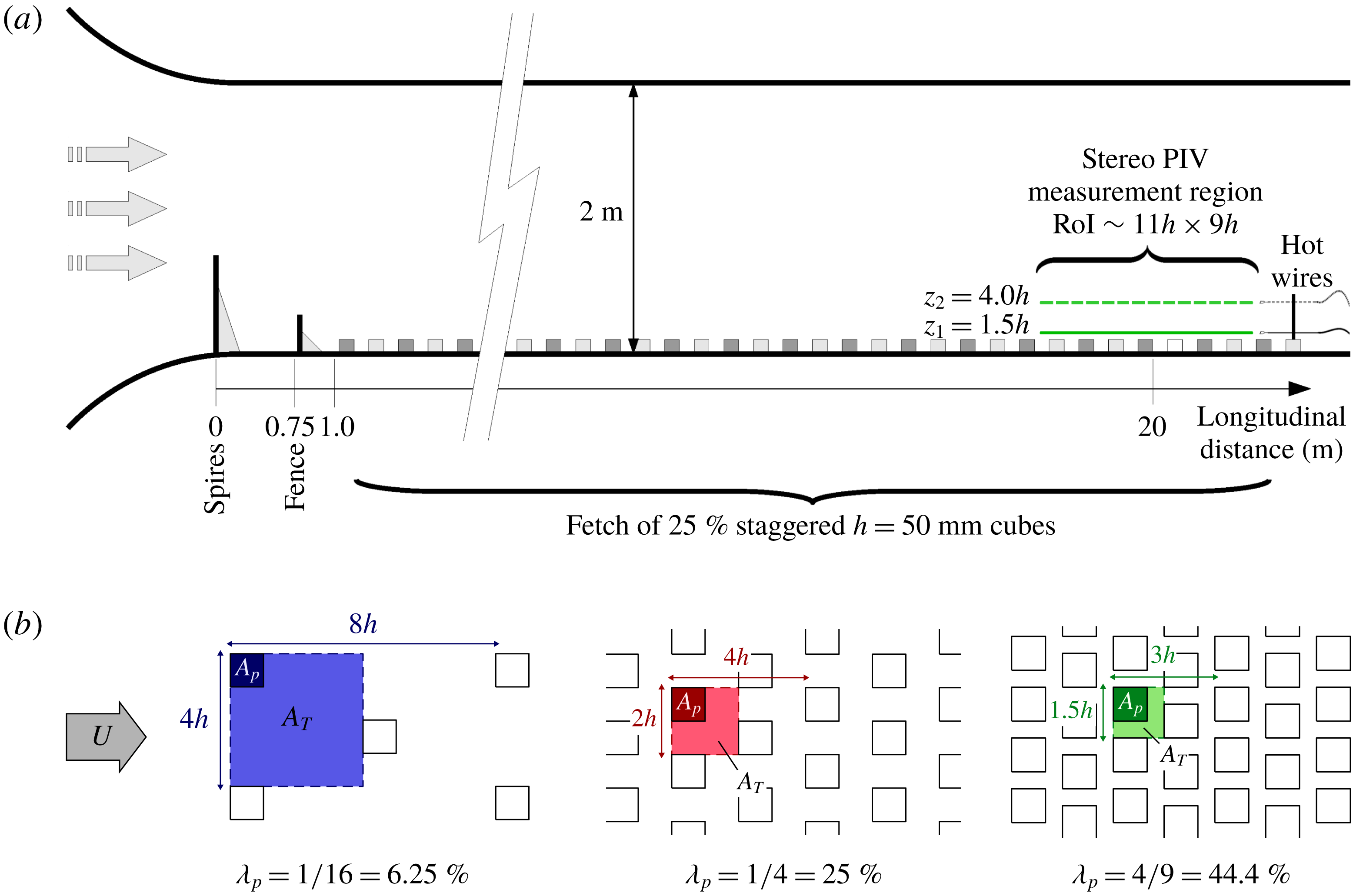
The experiments were conducted in the wind tunnel of the Laboratoire de recherche en Hydrodynamique, Energétique et Environnement Atmosphérique of Ecole Centrale de Nantes (LHEEA, Nantes, France), with a working section of dimensions
 $24~\text{m}\times 2~\text{m}\times 2~\text{m}$
(figure 1
a). The frame of reference
 $(\boldsymbol{e}_{x},\boldsymbol{e}_{y},\boldsymbol{e}_{z})$
is attached to the wind tunnel such that coordinates
 $x$
,
 $y$
and
 $z$
represent positions along the streamwise, spanwise and wall-normal directions, respectively. The boundary layer is tailored using five wall-normal tapered spires of 800 mm height and 134 mm width at their base, in conjunction with a 200 mm high solid fence spanning the working section and located 0.75 m downstream of the inlet. The flow then develops over an idealised urban canopy model consisting of a 22 m long fetch of staggered cubes of height
 $h=50$
mm. This layout is designed to maximise the thickness of the boundary layer,
 $\unicode[STIX]{x1D6FF}$
, defined as the height at which the mean streamwise velocity reaches 99 % of the free-stream velocity
 $U_{e}$
. The boundary layer is approximately 1 m thick at the measurement station when
 $U_{e}=5.7~\text{m}~\text{s}^{-1}$
. These conditions yield a high ratio
 $\unicode[STIX]{x1D6FF}/h>20$
and particularly high Reynolds numbers
 $\unicode[STIX]{x1D6FF}^{+}=U_{\unicode[STIX]{x1D70F}}\unicode[STIX]{x1D6FF}/\unicode[STIX]{x1D708}\sim 30\,000$
,
 $h^{+}=U_{\unicode[STIX]{x1D70F}}h/\unicode[STIX]{x1D708}\sim 1300$
, where
 $U_{\unicode[STIX]{x1D70F}}$
is the friction velocity,
 $\unicode[STIX]{x1D708}$
the kinematic viscosity and superscript
 $+$
denotes the inner scaling based on wall units
 $\unicode[STIX]{x1D708}/U_{\unicode[STIX]{x1D70F}}$
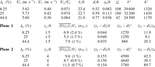
. Boundary layer characteristics are provided in table 1 and further discussion about their estimation is given in § 3.1.
Description of the experimental facility: (a) schematic of the atmospheric wind tunnel at laboratory LHEEA, Nantes, with the synchronised stereoscopic PIV/hot-wire anemometry set-up; (b) top view sketch of the three canopies, with the flow coming from the left. For each case the shaded region represents the staggered pattern; delimiting the area
 $A_{T}$
such that coverage is
 $\unicode[STIX]{x1D706}_{p}=A_{p}/A_{T}$
.

Characteristics of the boundary layer for the three canopy planar densities.

2.1 Flow configurations
Three plan densities are under study,
 $\unicode[STIX]{x1D706}_{p}=\{6.25\,\%,25\,\%,44.4\,\%\}$
, which cover the three types of real-life urban area, namely the isolated, wake-interference and skimming flow regimes, respectively (Oke Reference Oke1988). Figure 1(b) sketches the canopies and the corresponding periodic pattern. Here,
 $\unicode[STIX]{x1D706}_{p}=A_{p}/A_{T}$
where
 $A_{p}$
denotes the covered area and
 $A_{T}$
the total area in the pattern. The use of cubic elements leads to
 $\unicode[STIX]{x1D706}_{f}=\unicode[STIX]{x1D706}_{p}$
, as the frontal area
 $A_{f}$
of the cube is equal to the covered area
 $A_{p}$
. It should be noted that the other geometric parameters of the canopy are kept constant, e.g. a staggered arrangement of cubes of size
 $h=50$
mm. It is now well known that the aerodynamic parameters of the canopy, e.g. the roughness height
 $z_{0}$
and the displacement thickness
 $d$
, are strongly dependent on the canopy coverage (
 $\unicode[STIX]{x1D706}_{p},\unicode[STIX]{x1D706}_{f}$
), as reported for instance in Grimmond & Oke (Reference Grimmond and Oke1999). As reported in table 1 each canopy yields indeed to a different
 $z_{0}$
and an increasing
 $d$
with increasing
 $\unicode[STIX]{x1D706}_{p}$
(Macdonald et al.
Reference Macdonald, Griffiths and Hall1998; Kanda et al.
Reference Kanda, Moriwaki and Kasamatsu2004). In the following, results are consistently represented with regards to the three canopy densities: ▪
 $\unicode[STIX]{x1D706}_{p}=6.25\,\%$
, ●
 $\unicode[STIX]{x1D706}_{p}=25\,\%$
, ▴
 $\unicode[STIX]{x1D706}_{p}=44.4\,\%$
. Spanwise homogeneity of the flow has been assessed via streamwise velocity HWA measurements, spanning 1.3 m at both
 $z_{1}=1.5\,h$
and
 $z_{2}=4.0\,h$
. For the three canopy coverages, standard deviations of the mean value and the variance are below 3.5 % and 5.5 %, respectively. Pressure loss has been measured along the wind tunnel (Perret et al.
Reference Perret, Basley, Mathis and Piquet2019). Non-dimensional pressure gradient
 $-2.89\times 10^{-8}<K=(\unicode[STIX]{x1D708}/\unicode[STIX]{x1D70C}U_{e}^{3})(\text{d}P/\text{d}x)<-2.48\times 10^{-8}$
is small enough to have negligible impact on the development of the boundary layer (DeGraaff & Eaton Reference DeGraaff and Eaton2000).
2.2 Hot-wire anemometry
Fully time-resolved measurements were obtained through constant-temperature hot-wire anemometry (HWA) using
 $5~\unicode[STIX]{x03BC}\text{m}$
-diameter tungsten 1.25 mm long hot-wire probes (DANTEC-55P11 probe and DISA-55M01 anemometers).
In order to cover the full energy content, sufficiently long sample length of
 $T=5\times 20$
minutes (corresponding to boundary layer turnover times
 $TU_{e}/\unicode[STIX]{x1D6FF}\simeq 34\,000$
) was used with a sampling frequency
 $f_{hw}=10$
kHz (
 $\unicode[STIX]{x0394}T^{+}\simeq 1$
). To confirm the choice of the sampling parameters, the integral time scale of the flow
 $T_{u}(z_{1,2})$
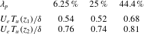
was calculated from HWA time series of streamwise velocity fluctuations at both wall-normal distances. The results – given in table 2 – show that the 100 min recorded for each case represent at least 40 000 integral time scales, which insures a high quality convergence. The integral time logically increases with the distance from the wall. It shows a noticeable increase in the case
 $\unicode[STIX]{x1D706}_{p}=44.4\,\%$
, which would suggest longer large-scale motions in this configuration.
For each canopy configuration, HWA time series were measured synchronously with the stereoscopic particle image velocimetry measurements (SPIV), and positioned downstream of SPIV planes at the same wall-normal location (see § 2.3). These datasets are complemented by HWA scans across the boundary layer to characterise the flow and conduct a two-point spectral coherence analysis in the lower part of the boundary layer. Using the measurements performed at the fixed point from this set of two-point measurements (13 independent runs for each flow configuration), the repeatability error was estimated as being 0.47 % and 0.89 % for
 $\langle U\rangle$
and
 $\langle \unicode[STIX]{x1D70E}_{u}^{2}\rangle$
, respectively. Based on a Gaussian assumption and the number of samples separated by one integral time scale
 $\unicode[STIX]{x1D6FF}/U_{e}$
, the statistical convergence error is 0.1 % and 0.87 % for
 $\langle U\rangle$
and
 $\langle \unicode[STIX]{x1D70E}_{u}^{2}\rangle$
, respectively. Estimate of the accuracy of the spectral coherence is shown in figure 9(d). For a detailed description of these HWA datasets, the reader is referred to the work of Perret et al. (Reference Perret, Basley, Mathis and Piquet2019).
Dimensionless integral time scales for the three canopy planar densities.

2.3 Stereoscopic particle image velocimetry
Three-component two-dimensional SPIV measurements were conducted in streamwise–spanwise planes (figure 1
a) using two
 $2048\times 2048$
pixel cameras FlowSense, positioned at forward scattering angles
 $\unicode[STIX]{x1D6FC}=\{20^{\circ },53^{\circ }\}$
and associated with 60 mm and 105 mm Nikkor lenses (at aperture
 $f_{\#}=2.8$
). The laser sheet was produced by a Nd-Yag laser (532 nm,
 $200~\text{mJ}~\text{cavity}^{-1}$
); its thickness was estimated to be between 3 and 5 mm. Two wall-normal locations were investigated independently:
 $z_{1}=1.5\,h$
and
 $z_{2}=4\,h$
(figure 1
a), respectively within the RSL and in the inertial region, as demonstrated in § 3.1 (Cheng & Castro Reference Cheng and Castro2002; Placidi & Ganapathisubramani Reference Placidi and Ganapathisubramani2015; Perret et al.
Reference Perret, Basley, Mathis and Piquet2019). Cross-correlation was performed in
 $32\times 32$
pixel windows, yielding approximately
 $20\times 12$
vectors/
 $h^{2}$
over a region of interest (RoI) of
 $11h\times 10h$
(or
 $0.55\unicode[STIX]{x1D6FF}\times 0.5\unicode[STIX]{x1D6FF}$
), which encompasses both the largest scales of the flow and the obstacle-induced coherent structures. The trade-off favouring the extension of the RoI naturally impacts the resolution of the smallest scales of the spectrum up to
 $0.015\unicode[STIX]{x1D6FF}$
, as shown in § 2.4 compared to hot-wire measurements. Dynamic Studio software provides a precision of
 $1/32\text{th}$
pixel on the cross-correlation peak. Up to 5 % outliers were detected in raw velocity fields. Mainly located along the edges of the RoI, these outliers were replaced using a
 $3\times 3$
-window median filter. The rest of the random noise polluting the smallest scales of the flow was reduced using a low-pass
 $3\times 3$
-window Gaussian filter after stereoscopic reconstruction. As for biased errors originating from SPIV projection, discrepancies in the wall-normal position of the laser sheet or background artefacts in particle images, their cumulative extent was estimated using the spatial dispersion of statistics between canopy patterns. The mean flow is periodic with respect to the canopy within a 2.5 % accuracy, and the turbulent kinetic energy within 4 %.
For each of the six configurations (three canopy densities
 $\unicode[STIX]{x1D706}_{p}=\{6.25\,\%,25\,\%,44.4\,\%\}$
at two wall distances
 $z_{1,2}$
), five independent series of 2100 velocity fields were acquired at
 $f_{spiv}=7$
Hz. These datasets of
 $N_{s}=10\,500$
samples were designed so as to resolve both statistically and spatially the large-scale motions (LSMs) of the flow. Statistical convergence is assured with a total acquisition span of 1500 s, comprising at least 10 000 integral time scales (table 2). At the same time, the snapshot sampling rate is high enough (
 $\unicode[STIX]{x0394}t_{spiv}=0.14\text{s}\lesssim T_{u}$
) and the RoI is large enough to enable streamwise combination of successive SPIV velocity fields by applying Taylor’s approximation, as detailed in § 2.4.
In the following, sample (i.e. time) and space averages of a given dataset
 $\{q_{k}(x,y)\}$
with
 $k=1,2,\ldots ,N_{s}$
are denoted respectively
 $\langle q\rangle (x,y)$
and
 $\overline{q_{k}}$
. Mean flow
 $\langle \boldsymbol{U}\rangle (x,y)$
results from the sample average of velocity fields
 $\{\boldsymbol{U}_{k}(x,y)\}$
, so that each instantaneous field can be decomposed as
 $$\begin{eqnarray}\boldsymbol{U}_{k}(x,y)=\langle \boldsymbol{U}\rangle (x,y)+\boldsymbol{u}_{k}(x,y)=(\langle U\rangle +u_{k})\boldsymbol{e}_{x}+(\langle V\rangle +v_{k})\boldsymbol{e}_{y}+(\langle W\rangle +w_{k})\boldsymbol{e}_{z},\end{eqnarray}$$
where
 $\boldsymbol{u}_{k}(x,y)$
is the fluctuating field.
2.4 Reconstructed streamwise large-scale dynamics using Taylor approximation
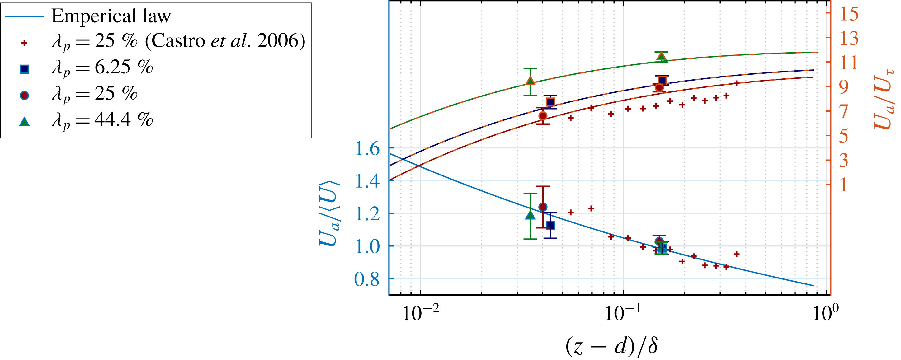
The approximation of frozen turbulence (Taylor Reference Taylor1938) entails the existence of a constant scale-independent advection velocity, below named
 $U_{a}$
. Such an assumption requires the flow to be statistically uniform, both in space (homogeneous) and time (permanent regime). The permanent regime is ensured with constant experimental conditions (
 $U_{e}=cst\pm 1\,\%$
) and § 3.2 will show that the statistical properties of the flow change very little in space in the two streamwise–spanwise planes under investigation – at
 $z_{1,2}=\{1.5h,4h\}$
. Therefore the advection velocity is assumed to be constant in a streamwise–spanwise plane
 $(x,y)$
, that is, a function solely of the distance from the wall.
 $U_{a}(z)$
is estimated relying on space–time correlations between SPIV and synchronised HWA data. The reader may refer to appendix A for further details regarding the methodology.
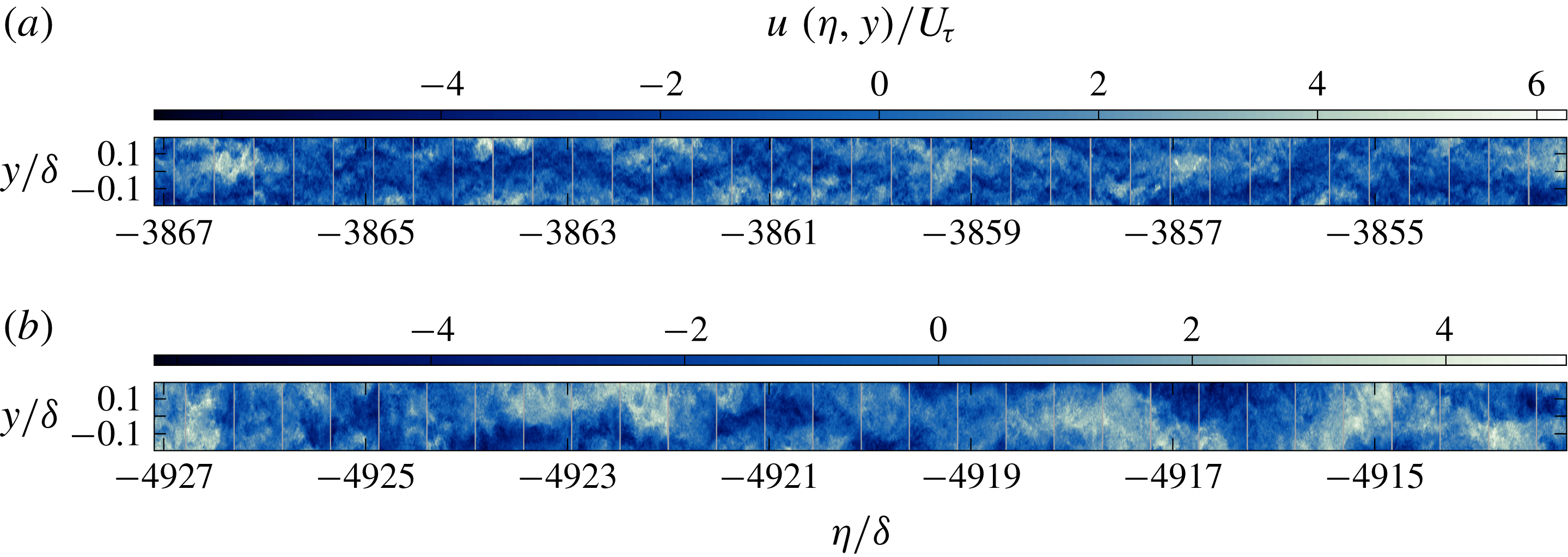
Excerpts of streamwise velocity fluctuations
 $u(\unicode[STIX]{x1D702},y)/U_{\unicode[STIX]{x1D70F}}$
in combined SPIV fields for canopy
 $\unicode[STIX]{x1D706}_{p}=6.25\,\%$
in (a)
 $z_{1}=1.5\,h$
and (b)
 $z_{2}=4.0\,h$
(vertical grey lines mark field junctions).

Using the advection velocity allows us to combine successive SPIV snapshots into a unique fluctuating velocity field (Dennis & Nickels Reference Dennis and Nickels2011; Basley, Perret & Mathis Reference Basley, Perret and Mathis2018), for which, at a given wall-normal distance
 $z$
(the dependence on
 $z$
is omitted below for brevity) streamwise position and time are equivalent. This gives
 $$\begin{eqnarray}\boldsymbol{u}(\unicode[STIX]{x1D702},y)=\boldsymbol{u}(t_{\unicode[STIX]{x1D702}},y)=\boldsymbol{u}_{k}(x_{spiv},y),\quad \text{with}~k=\{1,\ldots ,N_{s}\},\end{eqnarray}$$
with the new streamwise and time coordinates,
 $\unicode[STIX]{x1D702}$
and
 $t_{\unicode[STIX]{x1D702}}$
, being obtained from coordinate
 $x_{spiv}$
in the SPIV fields and advection velocity
 $U_{a}$
as follows
 $$\begin{eqnarray}\unicode[STIX]{x1D702}=x_{spiv}-U_{a}(k-1)\unicode[STIX]{x0394}t_{spiv},\quad t_{\unicode[STIX]{x1D702}}=-\frac{\unicode[STIX]{x1D702}}{U_{a}},\quad \text{with}~k=\{1,\ldots ,N_{s}\}.\end{eqnarray}$$
The reconstructed field
 $\boldsymbol{u}(\unicode[STIX]{x1D702},y)$
resolves large streamwise length scales far beyond the original extension of the SPIV fields. To illustrate this process, excerpts from combined fields
 $u_{T}$
are shown in figure 2(a,b) for the sparse canopy
 $\unicode[STIX]{x1D706}_{p}=6.25\,\%$
. The continuity of the resulting field is quite convincing with regards to the largest scales of the flow. For scales such that
 $\unicode[STIX]{x1D706}>\unicode[STIX]{x1D6FF}$
, cross-correlation functions between HWA and streamwise-extended velocity fields reach over 0.7 and 0.9 at
 $z_{1}=1.5\,h$
and
 $z_{2}=4.0\,h$
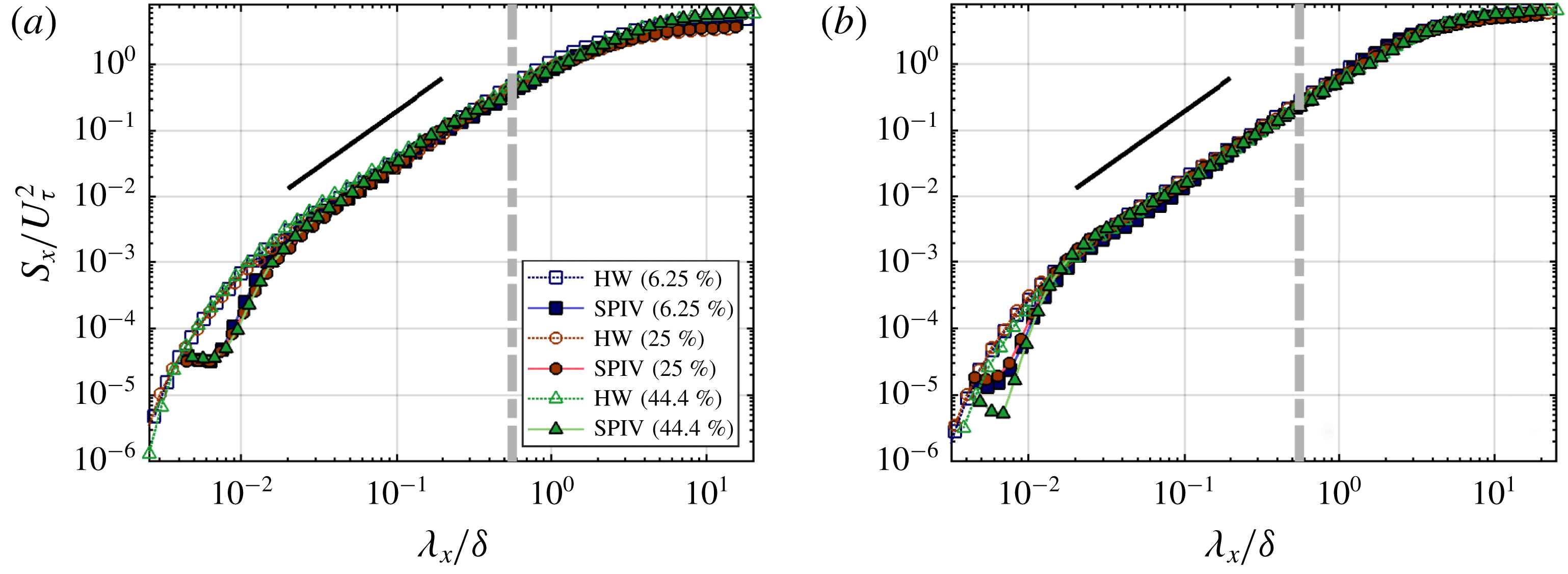
, respectively. This high level of correlation demonstrates the relevance of Taylor’s approximation and the quality of the reconstructed large-scale dynamics for all canopies under consideration. The validation of the reconstructed dynamics is also carried out in spectral space in figure 3. Power spectral densities from both SPIV and HWA data match well for
 $\unicode[STIX]{x1D706}_{x}>0.015\unicode[STIX]{x1D6FF}$
, that is including the extension to streamwise wavelengths
 $\unicode[STIX]{x1D706}_{x}>0.55\unicode[STIX]{x1D6FF}=L_{x}$
, obtained using Taylor’s approximation. At smaller streamwise wavelengths, discrepancies exist due to the limited spatial resolution of the present SPIV experiments.
Streamwise power spectral densities of both hot-wire time series and combined SPIV snapshots are compared using Taylor’s approximation, at
 $z_{1}=1.5\,h$
(a) and
 $z_{2}=4.0\,h$
(b). Spectra are computed and averaged over 1500, 50 %-overlapped 2 s long windows. The grey dash-dot line marks SPIV fields streamwise extension
 $L_{x}=11h=0.55\unicode[STIX]{x1D6FF}$
and the black slope represents the
 $5/3$
power law.

3 Results and discussion
In this section, experimental results obtained for the three canopy configurations are analysed to determine how the change in geometry impacts on the spatial organisation of the flow. Boundary layer characteristics are the focus of § 3.1 while local statistics, moments and shear stresses, are investigated throughout the streamwise–spanwise planes at
 $z_{1}=1.5\,h$
and
 $z_{2}=4.0\,h$
in § 3.2. The subsequent paragraphs are devoted to the identification of coherent structures through a detailed spectral analysis of the flow.
3.1 Characterisation of the boundary layer
Aerodynamic parameters of the wall-bounded flow for all three canopy configurations were deduced from form drag measurements and streamwise velocity profiles
 $\langle U\rangle (z)$
. Both displacement thickness
 $d$
and friction velocity
 $U_{\unicode[STIX]{x1D70F}}$
were estimated using pressure measurements around a cube within the canopy (Cheng et al.
Reference Cheng, Hayden, Robins and Castro2007). Hot-wire measurements of streamwise velocity
 $U(z,t)$
were acquired across the boundary layer from
 $1.2\,h\leqslant z\leqslant 30\,h\sim 1.4\,\unicode[STIX]{x1D6FF}$
to identify roughness length
 $z_{0}$
from the logarithmic law
 $$\begin{eqnarray}\langle U\rangle ^{+}=\frac{\langle U\rangle }{U_{\unicode[STIX]{x1D70F}}}=\frac{1}{\unicode[STIX]{x1D705}}\ln \left(\frac{z-d}{z_{0}}\right),\end{eqnarray}$$
with the von Kármán constant
 $\unicode[STIX]{x1D705}$
set to 0.4. The basic properties of the boundary layer are reported here in table 1. Note that (3.1) assumes the uniformity of the mean flow at a given wall distance
 $z$
but that assumption is only valid outside the RSL. For all flow configurations,
 $z_{0}^{+}$
is between 40 and 160, a range well above the critical value of
 $z_{0c}^{+}=0.5$
reported by Snyder & Castro (Reference Snyder and Castro2002) to ensure that the flow is in the fully rough regime. Moreover, all the global characteristics of the investigated boundary layer (such as
 $U_{\unicode[STIX]{x1D70F}}/U_{e}$
,
 $d/h$
and
 $z_{0}/h$
, as reported in table 1) are independent of the flow Reynolds number
 $\unicode[STIX]{x1D6FF}^{+}$
(not shown here, the reader is referred to Perret et al.
Reference Perret, Basley, Mathis and Piquet2019) and consistent with values from the literature (Kanda et al.
Reference Kanda, Moriwaki and Kasamatsu2004; Cheng et al.
Reference Cheng, Hayden, Robins and Castro2007; Kanda et al.
Reference Kanda, Kanega, Kawai, Moriwaki and Sugawara2007; Hagishima et al.
Reference Hagishima, Tanimoto, Nagayama and Meno2009; Leonardi & Castro Reference Leonardi and Castro2010; Ahn et al.
Reference Ahn, Lee and Sung2013), indicating that the flows have reached the fully rough regime (Jiménez Reference Jiménez2004).
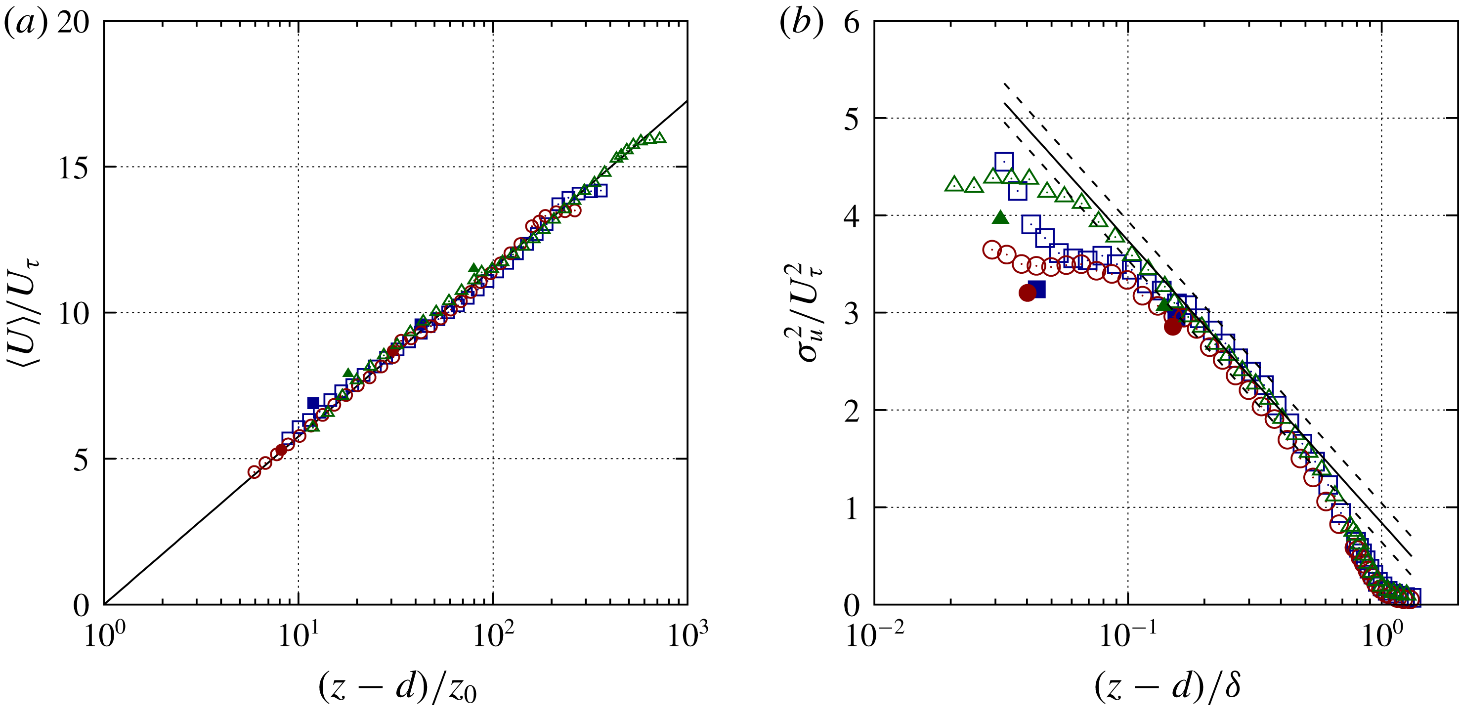
Wall-normal profiles of (a) mean streamwise velocity component and (b) variance of the streamwise velocity component, compiling (filled symbols) present study and (open symbols) hot-wire measurements from Perret et al. (Reference Perret, Basley, Mathis and Piquet2019). The solid black line in (a) shows the logarithmic law for the mean streamwise velocity component (3.1). The solid black line in (b) corresponds to the logarithmic law for the variance with a slope
 $A_{1}=1.26$
(3.2) while the dashed black lines show a range
 $\unicode[STIX]{x1D70E}_{u}^{2}/U_{\unicode[STIX]{x1D70F}}^{2}\pm 0.2$
as in Squire et al. (Reference Squire, Morill-Winter, Hutchins, Schultz, Klewicki and Marusic2016).

The present boundary layer developing over approximately twenty metres allows for the existence of an unambiguous log layer in all investigated cases. This is most notably shown in figure 4, where wall-normal profiles exhibit a log-law similarity over more than one order of magnitude. Additionally, the diagnostic plot from Castro, Segalini & Alfredsson (Reference Castro, Segalini and Alfredsson2013) has been used to validate the characteristics of the flows in Perret et al. (Reference Perret, Basley, Mathis and Piquet2019).
Good concordance is observed between the present SPIV campaign and hot-wire profiles in the logarithmic layer. Closer to the canopy, the lowest spatial resolution of the SPIV measurements leads to a slight underestimation of the variance.
One can note here the very good agreement between the variance profiles measured in the three investigated flows and the logarithmic law for the variance of the streamwise velocity component proposed by Marusic et al. (Reference Marusic, Monty, Hultmark and Smits2013), namely
 $$\begin{eqnarray}\frac{\unicode[STIX]{x1D70E}_{u}^{2}}{U_{\unicode[STIX]{x1D70F}}^{2}}=B_{1}-A_{1}\ln \left(\frac{z-d}{\unicode[STIX]{x1D6FF}}\right),\end{eqnarray}$$
where
 $B_{1}$
is a constant that depends on the flow geometry and wake parameter and
 $A_{1}=1.26$
is the slope constant proposed by Marusic et al. (Reference Marusic, Monty, Hultmark and Smits2013). Townsend (Reference Townsend1976) showed that the presence of self-similar wall-attached eddies in the inertial layer leads to the logarithmic wall-normal evolution of both the variance and the mean of the streamwise velocity component. Thus, the overall good collapse of the present results with this theoretical prediction confirms the well-developed high Reynolds number character of the investigated flows, without any unwanted effect of the spires on the variance wall-normal evolution and suggests that the structure of the flow over large roughness elements can be expected to match that of conventionally developing flows. Lastly, the departure from this logarithmic law in the region close to the canopy top can serve as an estimate for the bottom limit of the inertial layer, hence the upper limit of the RSL (Squire et al.
Reference Squire, Morill-Winter, Hutchins, Schultz, Klewicki and Marusic2016). When accounting for the possible scatter of experimental data and the error in estimating
 $B_{1}$
via the use of a range of validity of
 $\unicode[STIX]{x1D70E}_{u}^{2}/U_{\unicode[STIX]{x1D70F}}^{2}\pm 0.2$
(Squire et al.
Reference Squire, Morill-Winter, Hutchins, Schultz, Klewicki and Marusic2016), it is clear that the two horizontal planes at
 $z_{1}=1.5\,h$
and
 $z_{2}=4.0\,h$
where the SPIV measurements were performed are located in the RSL and in the logarithmic layer, respectively.
3.2 Statistical heterogeneity in streamwise–spanwise planes
 $(x,y)$

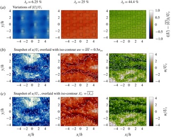
A global view of the influence of the different canopy density is illustrated in figure 5 with mean flow and an example of the fluctuating velocity field for each canopy configuration in the RSL region at
 $z_{1}=1.5\,h$
. The mean streamwise velocity component is quasi-uniform across the field (figure 5
a), with only a slight signature of the cubes in the isolated regime (
 $\unicode[STIX]{x1D706}_{p}=6.25\,\%$
). On the other hand, velocity fluctuations exhibit streaky large-scale motions (LSMs), characteristic of turbulent boundary layers, bearing no apparent dependency to the canopies. The LSMs are associated with sweeping and ejecting features revealed by negative fluctuations of wall-normal shear stress
 $uw$
(figure 5
b). Small-scale coherent structures are featured in figure 5(c), where wall-normal eddies are highlighted through swirling strength
 $\unicode[STIX]{x1D706}_{ci}$
defined as (Adrian et al.
Reference Adrian, Christensen and Liu2000):
 $$\begin{eqnarray}\unicode[STIX]{x1D706}_{ci}=\left|\text{Im}\left(\text{eig}\left(\frac{\unicode[STIX]{x2202}u_{i}}{\unicode[STIX]{x2202}x_{j}}\right)\right)\right|\quad \text{and using planar vorticity}~\unicode[STIX]{x1D714}_{z},\unicode[STIX]{x1D706}_{ci}^{s}=\unicode[STIX]{x1D706}_{ci}\,\text{sign}(\unicode[STIX]{x1D714}_{z}).\end{eqnarray}$$
Eddies are distributed in regions of strong shear alongside and between LSMs rather than attached to the canopy obstacles (Coceal et al. Reference Coceal, Dobre, Thomas and Belcher2007).
Reynolds decomposition of SPIV datasets in plane
 $z_{1}=1.5\,h$
for all three canopy configurations: colour scales represent (a) variations of mean flow streamwise component
 $(\langle U\rangle -\overline{\langle U\rangle })/U_{\unicode[STIX]{x1D70F}}$
and (b,c) the fluctuating streamwise velocity
 $u/U_{\unicode[STIX]{x1D70F}}$
for one snapshot. Solid white contour lines depict respectively intense negative levels of wall-normal shear stress
 $uw=\overline{uw}-\unicode[STIX]{x1D70E}_{uw}/2$
in (b), and intense positive levels of vortices vorticity signed swirling strength
 $\unicode[STIX]{x1D706}_{ci}^{s}=\overline{\langle \unicode[STIX]{x1D706}_{ci}\rangle }$
in (c).

The local influence of the canopy is investigated in both streamwise–spanwise planes. In the following, it is qualitatively linked to the three different flow regimes identified by Grimmond & Oke (Reference Grimmond and Oke1999) using the values of
 $\unicode[STIX]{x1D706}_{p}$
,
 $d/h$
and
 $z_{0}/h$
(table 1). This empirical approach is the only possible here in the absence of detailed flow measurements around the roughness obstacles as a function of
 $\unicode[STIX]{x1D706}_{p}$
as in Leonardi et al. (Reference Leonardi, Orlandi, Smalley, Djenidi and Antonia2003) for instance. Figure 6 compiles the spatial dispersion of several dimensionless moments. At the wall distance
 $z_{2}=4.0\,h$
, all statistics are basically uniform in space. Dispersion is generally below 2 %, except for shear stress
 $\langle uw\rangle$
which attains 5 % due to higher noise levels in SPIV images. This overall homogeneity confirms the roughness sublayer has ended at that point. As for the plane
 $z_{1}=1.5\,h$
, the proximity of the canopy does induce local variability of the statistical quantities. However, the results shown for
 $\unicode[STIX]{x1D706}_{p}=44.4\,\%$
are similar in magnitude to those observed at
 $z_{2}=4.0\,h$
, approximately 6 % for
 $\langle uw\rangle$
and almost unnoticeable otherwise. This implies that the outer edge of the RSL is close to
 $(z_{1}-d)/h=0.73$
in the skimming flow regime. Spatial heterogeneity increases slightly in the wake-interaction regime
 $\unicode[STIX]{x1D706}_{p}=25\,\%$
and is at its highest level in the isolated regime
 $\unicode[STIX]{x1D706}_{p}=6.25\,\%$
. It remains below 5 % for most of the statistical quantities except for the Reynolds shear stress
 $\langle uw\rangle$
which shows higher deviations to the space average, reaching just over 10 % for
 $\unicode[STIX]{x1D706}_{p}=6.25\,\%$
. The fact that roughness heterogeneity impacts more particularly on
 $\langle uw\rangle$
is consistent with observations of Raupach, Hughes & Cleugh (Reference Raupach, Hughes and Cleugh2006) in the case of sparse clustered roughness.
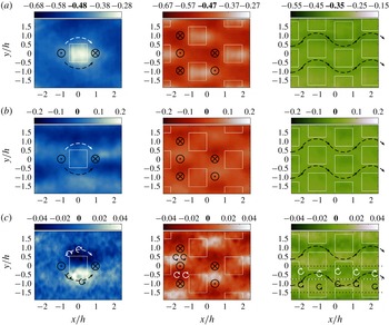
The impact of the canopy pattern on the statistical heterogeneity of the flow in the RSL is investigated using pattern-averaged maps in the plane
 $z_{1}=1.5\,h$
. Since the SPIV region of interest encompasses several (statistically equivalent) periodic patterns of the canopy, one can average the local statistics over 3, 10 and 12 smaller fields for
 $\unicode[STIX]{x1D706}_{p}=6.25\,\%$
, 25 % and 44.4 %, respectively, as shown in figure 7. Only the statistical moments exhibiting salient features associated with the canopy pattern are presented. Regarding the wall-normal shear stress
 $\langle uw\rangle$
, the denser canopy
 $\unicode[STIX]{x1D706}_{p}=44.4\,\%$
shows no significant spatial variability correlated with the geometry of the canopy (skimming regime). With the two lower densities
 $\unicode[STIX]{x1D706}_{p}=\{6.25\,\%,25\,\%\}$
, there is a slight decrease of
 $\langle uw\rangle$
directly above each obstacle. This corresponds to ejections and sweeps being on average less intense or less frequent above the cubes than around them, where exchange with the canopy inner flow takes place. It must be noted that the spatial average
 $\overline{\langle uw\rangle }$
is underestimated relatively to results from hot-wire or laser Doppler anemometry measurements (Cheng & Castro Reference Cheng and Castro2002; Castro et al.
Reference Castro, Cheng and Reynolds2006; Amir & Castro Reference Amir and Castro2011; Florens, Eiff & Moulin Reference Florens, Eiff and Moulin2013), likely because of the low-pass filtering inherent to mildly resolved SPIV, particularly for the reconstructed component. This translates into a reduced anti-correlation of
 $w$
with
 $u$
at the small scales.
Spatial standard deviation of statistical quantities at
 $z_{1}=1.5\,h$
(background, dark) and
 $z_{2}=4.0\,h$
(foreground, light), for the three canopy densities:
 $\unicode[STIX]{x1D706}_{p}=6.25\,\%$
(left bar), 25 % (centre bar) and 44.4 % (right bar).

Pattern-averaged statistics in plane
 $z_{1}=1.5\,h$
for the three densities, from left to right
 $\unicode[STIX]{x1D706}_{p}=6.25\,\%$
, 25 %, 44.4 %: (a) Reynolds shear stress
 $\langle uw\rangle /U_{\unicode[STIX]{x1D70F}}^{2}$
, (b) normalised skewness
 $\langle v^{3}\rangle /\langle v^{2}\rangle ^{3/2}$
and (c) average signed swirling strength
 $\langle \unicode[STIX]{x1D706}_{ci}^{s}\rangle h/\overline{\langle U\rangle }$
, where salient features of positive or negative vorticity are sketched with
 $\circlearrowleft$
symbols, black and white respectively. Mean flow streamlines around the canopy obstacles are qualitatively represented with arrows throughout the maps (
 $\otimes$
downwards and
 $\odot$
upwards stream). Bold indicates the space-averaged value.

The symmetry of velocity fluctuations (figure 7
b) is spatially altered by the canopy. Spanwise velocity fluctuations
 $v$
are skewed for both
 $\unicode[STIX]{x1D706}_{p}=6.25\,\%$
and
 $\unicode[STIX]{x1D706}_{p}=25\,\%$
due to the deflection of the flow around the cubes. The same can be said about streamwise and wall-normal skewness (not shown here). The case
 $\unicode[STIX]{x1D706}_{p}=44.4\,\%$
shows negligible asymmetry throughout the field.
Finally, the averaged swirling strength signed by vorticity
 $\langle \unicode[STIX]{x1D706}_{ci}^{s}\rangle$
(figure 7
c) allows us to identify statistically concentrated regions of negative and positive eddies. Let us point out that only non-null swirling strength values are considered in the averaging process. The three canopies exhibit very different organisations. The canopy 6.25 % yields a wake-like signature attached to every cube, that is consistent with vortices shed from upstream corners. It denotes a deflection of the flow by each (isolated) obstacle. On the other hand, the canopy 25 % presents a spatial distribution of eddies that can only be explained by the interaction with the recirculating flow inside the canopy (consistent with mean flow reported in DNS results by Coceal et al.
Reference Coceal, Dobre, Thomas and Belcher2007). The local effect of the canopy
 $\unicode[STIX]{x1D706}_{p}=44.4\,\%$
is almost unnoticeable. Nonetheless, one observes a distribution of wall-normal eddies slightly skewed alternatively positively and negatively following the curvature of the dominant flow within the canopy.
3.3 Evidence of self-similar eddies
The structure of the flow in the RSL and in the logarithmic layer is first investigated here using two-point HWA measurements performed with a fixed reference probe located at
 $z_{f}=5h$
and a moving probe at
 $1.25h<z_{m}<4h$
. Perret et al. (Reference Perret, Basley, Mathis and Piquet2019) have recently shown the presence of VLSMs in the same flow configurations as the present ones and their footprint onto the flow in the RSL, consistently with the recent findings of Lee et al. (Reference Lee, Sung and Krogstad2011) and Placidi & Ganapathisubramani (Reference Placidi and Ganapathisubramani2017) in similar rough-wall configurations. This point is not further addressed in the present work. The emphasis is on the presence of self-similar motions in highly roughened flows.
In light of the recent work of Baars, Hutchins & Marusic (Reference Baars, Hutchins and Marusic2017), the analysis relies on the spectral coherence across the boundary layer. The spectral coherence of the fluctuating streamwise velocity component
 $u$
between the two positions
 $z_{f}$
and
 $z_{m}$
is defined as:
 $$\begin{eqnarray}\unicode[STIX]{x1D6FE}^{2}(z_{f},z_{m},\unicode[STIX]{x1D706}_{x})=\frac{|\langle \hat{u} (\unicode[STIX]{x1D706}_{x},z_{f})\hat{u} ^{\ast }(\unicode[STIX]{x1D706}_{x},z_{m})\rangle |^{2}}{\langle |\hat{u} (\unicode[STIX]{x1D706}_{x},z_{f})|^{2}\rangle \,\langle |\hat{u} (\unicode[STIX]{x1D706}_{x},z_{m})|^{2}\rangle },\end{eqnarray}$$
where
 $\hat{u}$
denotes the Fourier transform of
 $u$
,
 $\hat{u} ^{\ast }$
its complex conjugate,
 $\langle \cdot \rangle$
the ensemble average and
 $|\hat{u} |$
the modulus of the complex number
 $\hat{u}$
. Here, the streamwise wavelength
 $\unicode[STIX]{x1D706}_{x}$
is calculated from the temporal frequency
 $f$
using Taylor’s hypothesis based on the mean streamwise velocity measured at
 $z=z_{m}$
as
 $\unicode[STIX]{x1D706}_{x}=\langle U(z_{m})\rangle /f$
. As introduced by Townsend (Reference Townsend1976) in his attached-eddy hypothesis, self-similar eddies can be described as a hierarchy of geometrically self-similar structures scalable with their distance from the wall (Perry, Henbest & Chong Reference Perry, Henbest and Chong1986; Baars et al.
Reference Baars, Hutchins and Marusic2017). In particular, self-similarity implies that both streamwise and spanwise scales of the structures evolve in the same manner as a function of the wall distance (i.e.
 $\unicode[STIX]{x1D706}_{y}\propto \unicode[STIX]{x1D706}_{x}$
). In the context of smooth-wall boundary layers, Baars et al. (Reference Baars, Hutchins and Marusic2017) have shown the link between the topography of the
 $\unicode[STIX]{x1D6FE}^{2}(z_{f},z_{m},\unicode[STIX]{x1D706}_{x})$
isocontours, the so-called coherence spectrogram, and the existence of self-similar eddies. Performing a conceptual reconstruction of the
 $\unicode[STIX]{x1D6FE}^{2}$
isocontours, these authors first showed that the
 $\unicode[STIX]{x1D6FE}^{2}$
isocontours should align with lines of constant
 $\unicode[STIX]{x1D706}_{x}/z$
within a triangular region in
 $(\unicode[STIX]{x1D706}_{x},z)$
-space. The second key result of their study is that, in the above-mentioned triangular region, the coherence magnitude should follow the scaling
 $$\begin{eqnarray}\unicode[STIX]{x1D6FE}^{2}=C_{1}\ln (\unicode[STIX]{x1D706}_{x}/z)+C_{2},\end{eqnarray}$$
where
 $C_{1}\approx 0.302$
and
 $C_{2}\approx -0.796$
are two empirically determined constants. It should be pointed out that these two results are consequences of the self-similarity of the supposed hierarchy of motions while the wall-attached character results from the choice of the location of the reference point
 $z_{f}$
used to calculate the spectral coherence in the near-wall region. For scales larger than an outer limit
 $\unicode[STIX]{x1D706}_{x}/\unicode[STIX]{x1D6FF}$
(of approximately 10 in their study), the coherence becomes scale independent, i.e.
 $\unicode[STIX]{x1D6FE}^{2}(\unicode[STIX]{x1D706}_{x})$
reaches an asymptotic value that depends on the considered wall-normal location
 $z_{m}$
. The inner limit in terms of wavelength of this region is given by the value of
 $\unicode[STIX]{x1D706}_{x}/z$
at which the relationships (3.5) gives
 $\unicode[STIX]{x1D6FE}^{2}=0$
. This also defines a streamwise/wall-normal aspect ratio of the self-similar structures as
 $\unicode[STIX]{x1D706}_{x}/z=\exp (-C_{2}/C_{1})\approx 14$
. Interestingly, Baars et al. (Reference Baars, Hutchins and Marusic2017) also pointed out that the self-similar character embodied by (3.5) implies that the coherence should behave as
 $\unicode[STIX]{x1D6FE}^{2}=-C_{1}\ln (z)+C_{3}$
in the scale-independent outer region. The intersect of the fit of this equation to the coherence spectrogram at a given large
 $\unicode[STIX]{x1D706}_{x}/z$
enabled them to define an upper limit of the self-similar region in terms of wall-normal distance, and using the above-defined structure aspect ratio, an upper limit in terms of streamwise structures extent
 $\unicode[STIX]{x1D706}_{x}$
.
Given that in the present case the fixed probe is located in the upper part of the logarithmic region (
 $z_{f}=5h$
), the distance
 $\unicode[STIX]{x1D6E5}_{z}=|z_{f}-z_{m}|$
between the reference probe and the moving probe is used as a scaling length instead of the wall-normal location
 $z$
in the case of Baars et al. (Reference Baars, Hutchins and Marusic2017). One obtains spectrograms
 $\unicode[STIX]{x1D6FE}^{2}(z_{f},\unicode[STIX]{x1D6E5}_{z},\unicode[STIX]{x1D706}_{x})$
, even if the dependence of
 $\unicode[STIX]{x1D6FE}^{2}$
on
 $z_{f}$
will be omitted for brevity, as only one reference wall-normal location is investigated. Note also that in the subsequent figures presenting the spectrograms of
 $\unicode[STIX]{x1D6FE}^{2}(\unicode[STIX]{x1D6E5}_{z},\unicode[STIX]{x1D706}_{x})$
, the wall-normal axis showing the dependence on
 $\unicode[STIX]{x1D6E5}_{z}$
has been reversed to reflect the fact that the reference point was located above the moving probe during the experiments (figure 8
d). This results in inverted figures compared to those of Baars et al. (Reference Baars, Hutchins and Marusic2017).
Spectrograms of coherence
 $\unicode[STIX]{x1D6FE}^{2}(\unicode[STIX]{x1D6E5}_{z},\unicode[STIX]{x1D706}_{x})$
for
 $\unicode[STIX]{x1D706}_{p}$
 $=$
(a) 6.25 %, (b) 25 % and (c) 44.4 % with contours from 0.05 to 0.85 with an increment of 0.1. Dashed lines represent two
 $\unicode[STIX]{x1D706}_{x}/\unicode[STIX]{x0394}z$
ratios, described in (a). (d) Schematic of the two-probe experimental set-up.

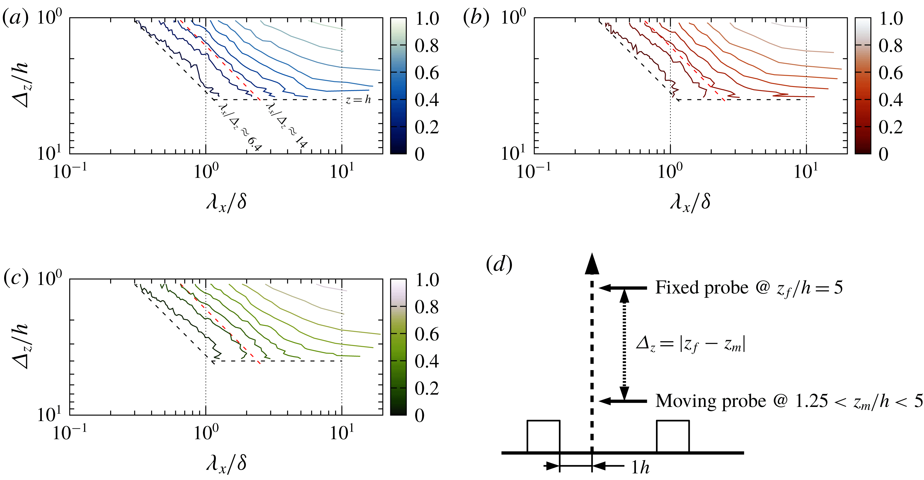
Coherence spectrograms obtained for the three different canopies are presented in figure 8. As for the smooth-wall configurations investigated by Baars et al. (Reference Baars, Hutchins and Marusic2017), they clearly display two distinct regions in
 $(\unicode[STIX]{x1D706}_{x},\unicode[STIX]{x1D6E5}_{z})$
-space. At large
 $\unicode[STIX]{x1D706}_{x}$
, isocontours of
 $\unicode[STIX]{x1D6FE}^{2}$
show a scale-independent behaviour with
 $\unicode[STIX]{x1D6FE}^{2}$
reaching an asymptotic value depending only on the considered separation
 $\unicode[STIX]{x1D6E5}_{z}$
. This confirms the existence of VLSMs whose size scales with outer variables, ranging deep into the RSL and primarily superimposed onto smaller-scale structures. A second region in which
 $\unicode[STIX]{x1D6FE}^{2}$
isocontours follow parallel straight lines is clearly visible at lower
 $\unicode[STIX]{x1D706}_{x}$
, in good agreement with the existence of the triangular region in the coherence spectrograms reported by Baars et al. (Reference Baars, Hutchins and Marusic2017). Existence of such a behaviour of the isocontours of
 $\unicode[STIX]{x1D6FE}^{2}$
evidences the presence of self-similar eddies in the logarithmic region of the investigated flows. In the present case, however, this region shows a trapezoidal shape rather than triangular. This difference is attributed to the choice of the reference location above the moving probe, a configuration in which the presence of the wall imposes an upper limit to the range of the wall-normal extent
 $\unicode[STIX]{x1D6E5}_{z}$
of the eddies. Another distinctive feature is the departure of the isocontours from the straight line behaviour for the lowest levels of coherence at large wall-normal separation
 $\unicode[STIX]{x1D6E5}_{z}$
for
 $1\lesssim \unicode[STIX]{x1D706}_{x}/\unicode[STIX]{x1D6FF}\lesssim 2$
, particularly for the
 $\unicode[STIX]{x1D706}_{p}=25$
and 44.4 % canopies (figure 8
b,c). Several hypotheses can be made to explain this discrepancy. Firstly, the adequacy of Taylor’s hypothesis in the near-canopy region might be questionable, which would result in an alteration of the shape of the isocontours. In the present study, the streamwise wavelength
 $\unicode[STIX]{x1D706}_{x}$
is computed from the temporal frequency using the local streamwise velocity component magnitude as an estimate for the convection velocity. However, several studies have shown the dependence of the convection velocity on the considered scale (Dennis & Nickels Reference Dennis and Nickels2008; Atkinson, Buchmann & Soria Reference Atkinson, Buchmann and Soria2015) and therefore the limitation of applicability of Taylor’s approximation. This could be an explanation for the above-mentioned departure. However, the fact that in the case of 6.25 % density, the contour shape is not altered tends not to favour this hypothesis. Secondly, the considered range of scale
 $\unicode[STIX]{x1D706}_{x}$
might not correspond to self-similar eddies but to a different type of structures of rather large wall-normal extent (at least
 $4h$
, the maximum probe separation), leaving a weak imprint onto the flow. However, these structures cannot be further investigated given the present two-point set-up. The use of a fixed probe close to the canopy and a moving probe above would be better suited.
Coherence spectra
 $\unicode[STIX]{x1D6FE}^{2}(\unicode[STIX]{x1D6E5}_{z},\unicode[STIX]{x1D706}_{x})$
for
 $\unicode[STIX]{x1D706}_{p}$
 $=$
(a) 6.25 %, (b) 25 % and (c) 44.4 %. The solid straight line corresponds to (3.5) with the same slope
 $C_{1}=0.302$
as Baars et al. (Reference Baars, Hutchins and Marusic2017) and an intercept of
 $C_{2}=-0.56$
. (d) Compensated coherence spectra
 $\tilde{\unicode[STIX]{x1D6FE}}^{2}(\unicode[STIX]{x1D6E5}_{z},\unicode[STIX]{x1D706}_{x})=\unicode[STIX]{x1D6FE}^{2}(\unicode[STIX]{x1D6E5}_{z},\unicode[STIX]{x1D706}_{x})-(C_{1}\ln (\unicode[STIX]{x1D706}_{x}/\unicode[STIX]{x1D6E5}_{z})+C_{2})$
for the three flow configurations (vertically shifted with increments of 0.3 for clarity). The vertical dashed line marks
 $\unicode[STIX]{x1D706}_{x}/\unicode[STIX]{x1D6E5}_{z}=\exp (-C_{2}/C_{1})$
at which (3.5) is zero. Line width corresponds to the 95 % confidence interval estimated as
 $\pm$
twice the standard deviation of
 $\unicode[STIX]{x1D6FE}^{2}(\unicode[STIX]{x1D6E5}_{z},\unicode[STIX]{x1D706}_{x})$
(Bendat & Piersol Reference Bendat and Piersol2010).

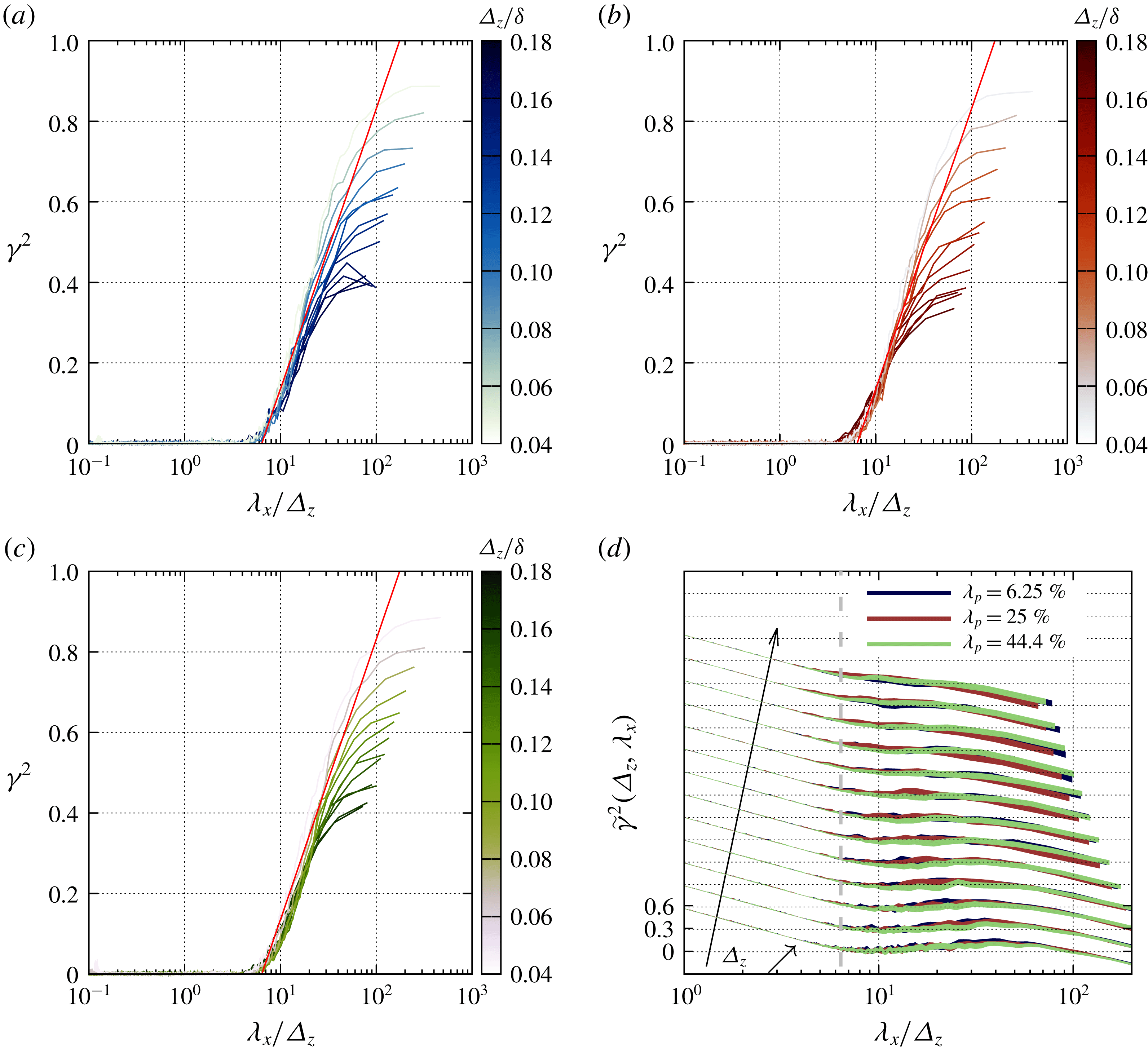
The presence of self-similar eddies is further confirmed for the three flow configurations by investigating the evolution of
 $\unicode[STIX]{x1D6FE}^{2}$
as a function of
 $\unicode[STIX]{x1D706}_{x}/\unicode[STIX]{x1D6E5}_{z}$
, which should correspond to (3.5) (in which the wall-normal distance
 $z$
must be replaced by the probe separation
 $\unicode[STIX]{x1D6E5}_{z}$
in the present case) (figures 9
a–c). The line following (3.5) is also displayed (solid red line) with its slope
 $C_{1}$
corresponding to that proposed by Baars et al. (Reference Baars, Hutchins and Marusic2017) while the intersect has been empirically adjusted to provide the best fit (
 $C_{2}=-0.56$
). While the slope
 $C_{1}=0.302$
leads to a remarkably good concordance, the change in
 $C_{2}$
implies a smaller streamwise/wall-normal aspect ratio of 6.4 compared to the value of 14 reported in smooth-wall configurations. Less elongated large-scale structures are indeed frequently reported in boundary layers over large roughness (Shaw et al.
Reference Shaw, Brunet, Finnigan and Raupach1995; Wu & Christensen Reference Wu and Christensen2010; Lee et al.
Reference Lee, Sung and Krogstad2011; Placidi & Ganapathisubramani Reference Placidi and Ganapathisubramani2017). To further investigate the presence of self-similar structures, the compensated spectral coherence
 $\tilde{\unicode[STIX]{x1D6FE}}^{2}(\unicode[STIX]{x1D6E5}_{z},\unicode[STIX]{x1D706}_{x})=\unicode[STIX]{x1D6FE}^{2}(\unicode[STIX]{x1D6E5}_{z},\unicode[STIX]{x1D706}_{x})-(C_{1}\ln (\unicode[STIX]{x1D706}_{x}/\unicode[STIX]{x1D6E5}_{z})+C_{2})$
is plotted in figure 9(d) as a function of
 $\unicode[STIX]{x1D706}_{x}/\unicode[STIX]{x1D6E5}_{z}$
. Any departure from the horizontal therefore corresponds to a discrepancy between the data and (3.5). Departure from the horizontal is visible for the three canopy densities, for the smallest and largest values of
 $\unicode[STIX]{x1D6E5}_{z}$
, with a larger and a smaller slope (even with the disappearance of a clear straight portion of the
 $\unicode[STIX]{x1D6FE}^{2}$
curve in semi-logarithmic plot) than
 $C_{1}$
, respectively. Intermediate values of wall-normal probe separation show coherence distribution in agreement with the fact that the logarithmic region is populated by self-similar eddies. The lack of concordance for moving points located closer to the canopy confirms the departure from the evolution of coherence isocontours in
 $(\unicode[STIX]{x1D706}_{x},\unicode[STIX]{x1D6E5}_{z})$
-space corresponding to the presence of self-similar eddies (figure 8). In the
 $\unicode[STIX]{x1D706}_{p}=44.4\,\%$
configuration, only the point closest to the canopy is affected by this departure whereas in the 6.25 % and 25 % flow configurations, a larger fraction of the near-canopy region seems to be altered. While the change of slope in the evolution of
 $\unicode[STIX]{x1D6FE}^{2}$
as a function of
 $\unicode[STIX]{x1D706}_{x}/\unicode[STIX]{x1D6E5}_{z}$
does not contradict the possible presence of self-similar eddies, it is worth noting that it implies a change of intersect and therefore of the streamwise/wall-normal aspect ratio of the eddies, the smaller the slope, the smaller the aspect ratio. Lines corresponding to aspect ratio of
 $\unicode[STIX]{x1D706}_{x}/\unicode[STIX]{x1D6E5}_{z}=6.4$
and 14 (inclined black and red dashed lines, respectively) are shown in figure 8. The smallest aspect ratio corresponds to the lowest level of coherence (0.05) and streamwise wavelength
 $\unicode[STIX]{x1D706}_{x}/\unicode[STIX]{x1D6FF}\approx 1$
at the location closest to the canopy (i.e. largest
 $\unicode[STIX]{x1D6E5}_{z}$
). This wavelength corresponds to that of the most energetics structures close to the canopy (see figure 11
a and Perret et al.
Reference Perret, Basley, Mathis and Piquet2019). The aspect ratio of 14 corresponds to higher levels of coherence and to
 $\unicode[STIX]{x1D706}_{x}/\unicode[STIX]{x1D6FF}\approx 3$
for the largest
 $\unicode[STIX]{x1D6E5}_{z}$
. This streamwise wavelength corresponds to that of the most energetic structures of the outer layer that have a strong imprint on the RSL (see figure 10
a and Perret et al.
Reference Perret, Basley, Mathis and Piquet2019). Again, the coexistence of various type of coherent structures of different streamwise extent is evidenced, which can be self-similar (i.e. of constant aspect ratio
 $\unicode[STIX]{x1D706}_{x}/\unicode[STIX]{x1D6E5}_{z}$
) or not as shown by the departure from the straight lines in figures 8 corresponding to a linear relationships between
 $\unicode[STIX]{x1D706}_{x}$
and
 $\unicode[STIX]{x1D6E5}_{z}$
. This confirms the greater complexity of flows developing over highly roughened surfaces, in which, in the range of scale-dependent spectral coherence, eddies of different nature may coexist in the near-wall region and the logarithmic region. Given the variety of the possible sources of discrepancy mentioned above and the limited amount of information available from the present two-point HWA database, the exact characterisation of the different structures present in the near-canopy region remains an open question.
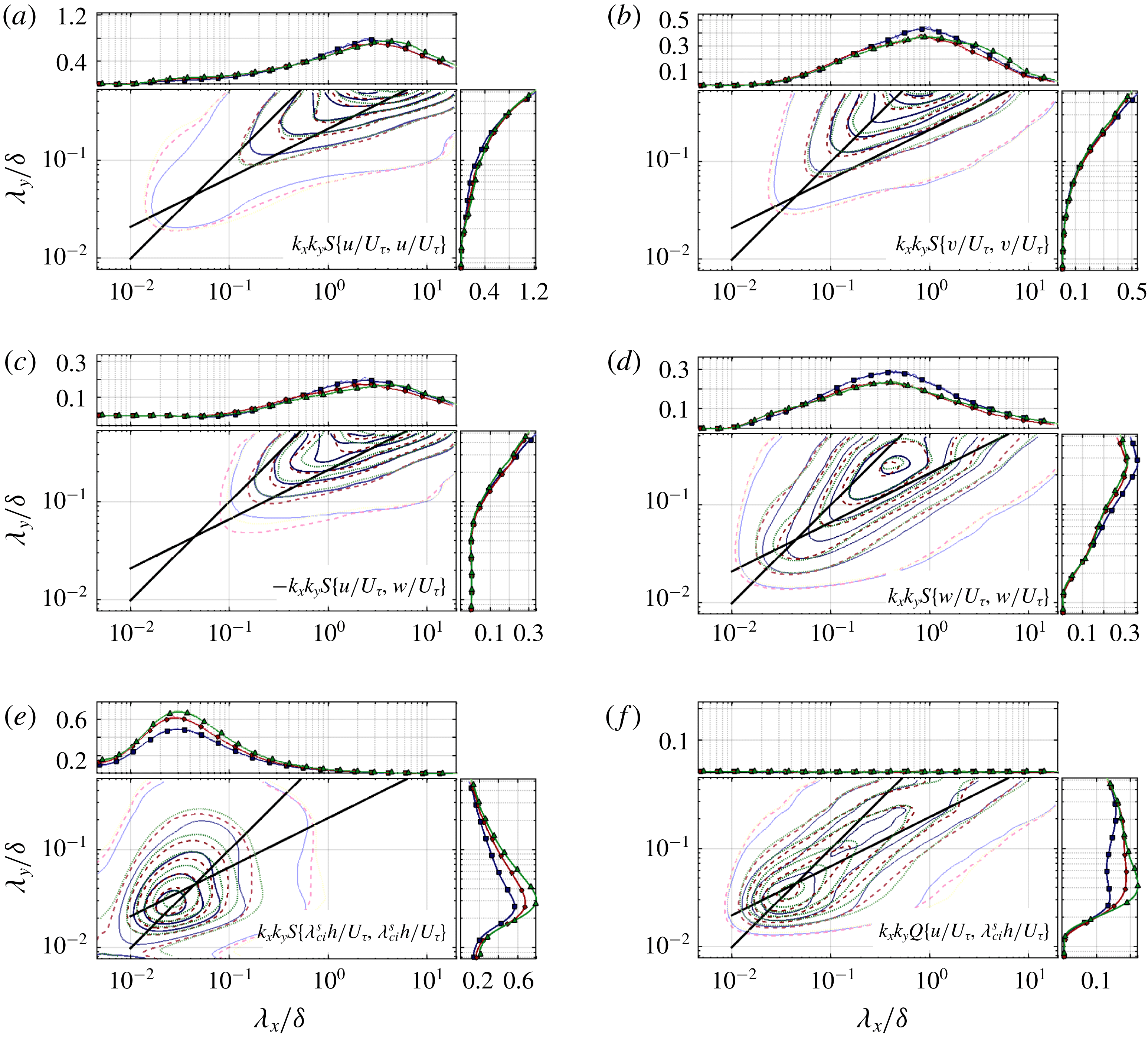
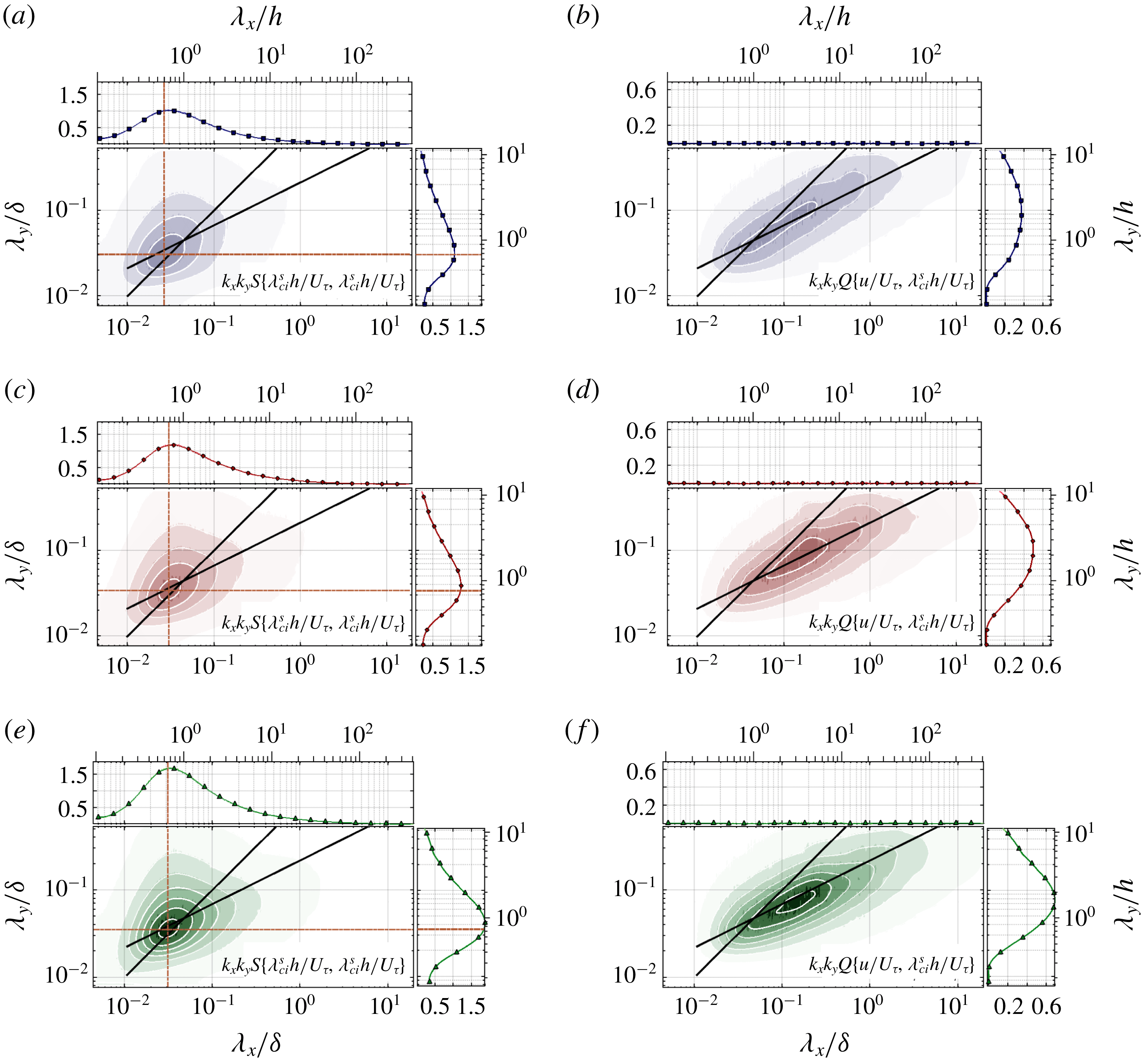
Pre-multiplied spectra in streamwise–spanwise plane
 $z_{2}=4.0\,h$
for (blue solid)
 $\unicode[STIX]{x1D706}_{p}=6.25\,\%$
, (red dashed)
 $\unicode[STIX]{x1D706}_{p}=25\,\%$
and (green dotted)
 $\unicode[STIX]{x1D706}_{p}=44.4\,\%$
are shown together with one-dimensional pre-multiplied spectra (same symbols as for previous figures). From top to bottom, (a,b)
 $k_{x}k_{y}S(u,u)$
and
 $k_{x}k_{y}S(v,v)$
; (c,d)
 $-k_{x}k_{y}S(u,w)$
and
 $k_{x}k_{y}S(w,w)$
; (e,f)
 $k_{x}k_{y}S(\unicode[STIX]{x1D706}_{ci}^{s},\unicode[STIX]{x1D706}_{ci}^{s})$
and
 $k_{x}k_{y}Q(u,\unicode[STIX]{x1D706}_{ci}^{s})$
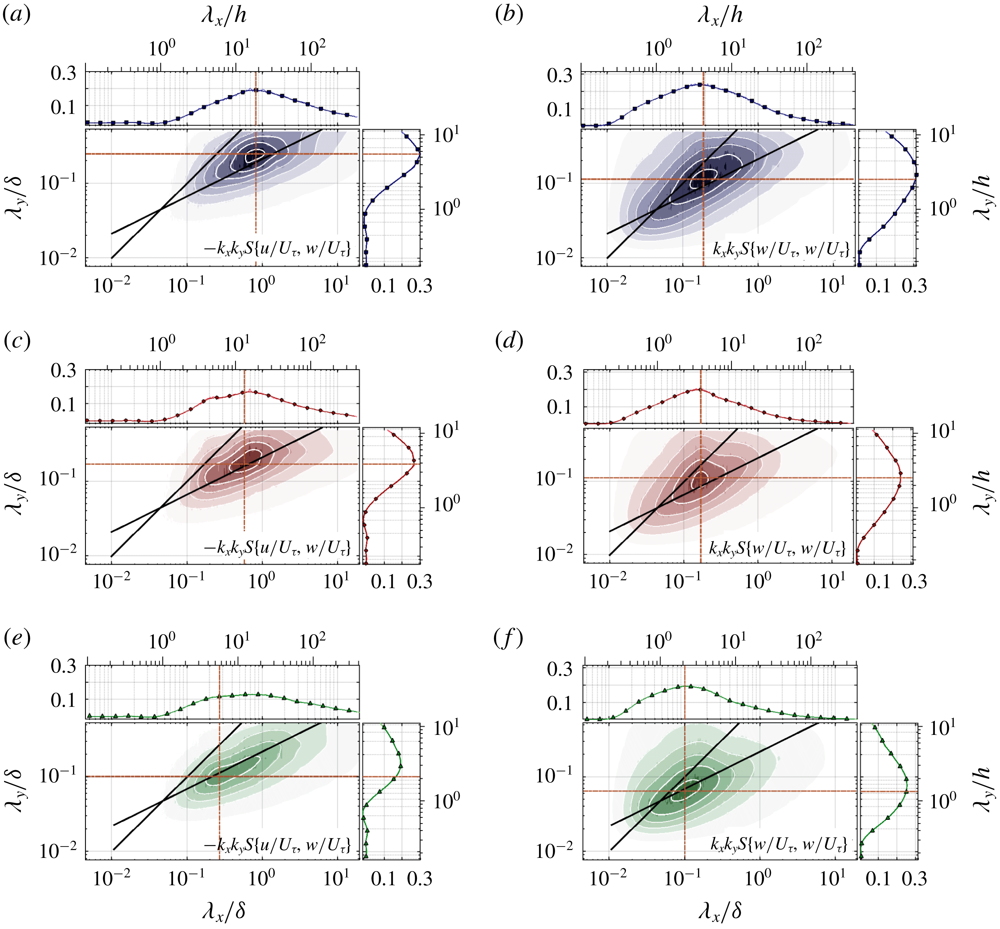
. Iso-levels are shown from 5 % to 95 % of the maximum with increments of 15 %. Solid black slopes mark
 $\unicode[STIX]{x1D706}_{x}=\unicode[STIX]{x1D706}_{y}$
and
 $\unicode[STIX]{x1D706}_{x}\propto \unicode[STIX]{x1D706}_{y}^{2}$
.

3.4 Spatial structure of the flow in the
$x{-}y$
plane

Having demonstrated evidence of the presence of self-similar eddies in the logarithmic layer for all roughness configurations, this section aims to identify the structuring length scales of the flow, resulting from the roughness-induced dynamics to the large-scale motions (LSMs) of the boundary layer. To that end, the Taylor-extended fluctuating velocity fields in both streamwise–spanwise planes
 $z_{1,2}=\{1.5h,4h\}$
were investigated through energy spectra, notably with respect to the influence of canopy coverage.
Power spectral densities are computed and averaged over windows of dimensions
 $(L_{x}^{\prime },L_{y})\simeq (20\unicode[STIX]{x1D6FF},0.5\unicode[STIX]{x1D6FF})$
with a 50 % overlap (Welch Reference Welch1967). The cross-spectrum between two fields
 $a$
and
 $b$
can be decomposed as
 $$\begin{eqnarray}P(a,b)=S(a,b)+\text{i}Q(a,b)=\langle \hat{a}\,\hat{b}^{\ast }\rangle ,\end{eqnarray}$$
where the co-spectrum
 $S$
is associated with in-phase correlated scales while the quadrature spectrum
 $Q$
represents correlated dynamics with a phase shift (Bendat & Piersol Reference Bendat and Piersol2010). In the following, one-dimensional spectra are identified with a subscript, e.g.
 $S_{x}$
for a co-spectrum along
 $\boldsymbol{e}_{x}$
, whereas their two-dimensional counterparts are simply referred to as
 $S$
and
 $Q$
. All spectra presented in figures 10 to 14 are pre-multiplied by wavenumbers
 $k_{x,y}=2\unicode[STIX]{x03C0}/\unicode[STIX]{x1D706}_{x,y}$
.
Spectra in the plane
 $z_{2}=4.0\,h$
are displayed in figure 10, showing a similar spectral signature for all cases, implying that the influence of the canopy remains strictly within the RSL and vanishes once above it. For the plane
 $z_{1}=1.5\,h$
, streamwise and spanwise velocities are featured in figure 11 and streamwise large scales are discussed with respect to temporal frequency scalings in figure 12. Wall-normal velocity spectra are shown in figure 13 and those of swirling strength in figure 14. The following sections discuss in depth the influence of the canopy on large-scale motions, sweeps, ejections and eddies within the inertial layer and the RSL.
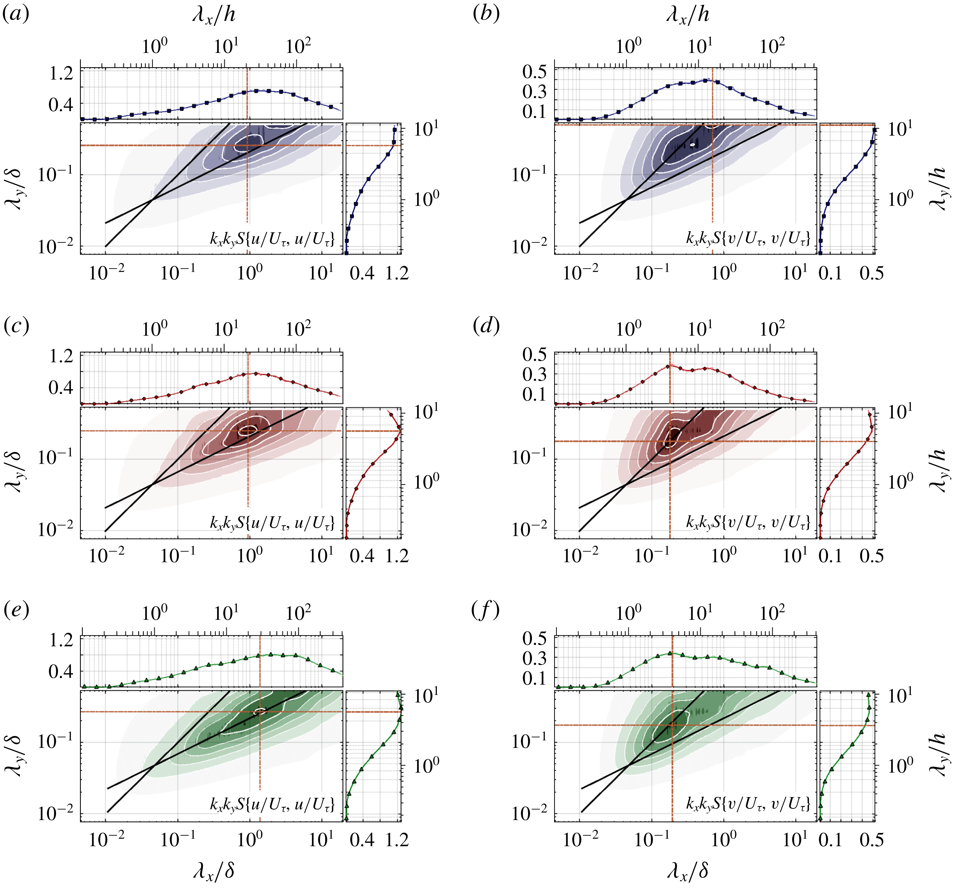
Pre-multiplied spectra in streamwise–spanwise plane
 $z_{1}=1.5\,h$
for (a,b)
 $\unicode[STIX]{x1D706}_{p}=6.25\,\%$
, (c,d)
 $\unicode[STIX]{x1D706}_{p}=25\,\%$
and (e,f)
 $\unicode[STIX]{x1D706}_{p}=44.4\,\%$
. From left to right, (a,c,e) auto-spectra
 $k_{x}k_{y}S(u,u)$
, and (b,d,f) auto-spectra
 $k_{x}k_{y}S(v,v)$
. Iso-levels are shown from 5 to 95 % of the maximum with steps of 15 %. Solid black slopes mark
 $\unicode[STIX]{x1D706}_{x}=\unicode[STIX]{x1D706}_{y}$
and
 $\unicode[STIX]{x1D706}_{x}\propto \unicode[STIX]{x1D706}_{y}^{2}$
. Raw spectra (colour maps) are smoothed (contour lines) for more clarity. Orange dash-dotted straight lines intersect at the maximum in the two-dimensional spectra.

3.4.1 Structures in the logarithmic layer
The spectral content of the logarithmic layer (i.e.
 $z_{2}=4.0\,h$
) and its relationship to the coherent structures already identified in the literature are first discussed here. The structures found in the RSL are the focus of subsequent sections. The first striking feature of the spectral characteristics in the logarithmic layer is their independence with regards to the canopy configuration (figure 10). Therefore, every comment that follows is valid for the three flow configurations. In agreement with previous works, the spectral signature of LSMs and VLSMs is mainly carried by the streamwise velocity and consists of a broad-band peak scaling with
 $\unicode[STIX]{x1D6FF}$
, centred around
 $\unicode[STIX]{x1D706}_{x}\sim 4\unicode[STIX]{x1D6FF}$
in the logarithmic layer (figure 10
a). Analysis of the two-dimensional spectrum of
 $u$
also shows the increasing anisotropy of the structures associated with scales up to
 $\unicode[STIX]{x1D706}_{x}/\unicode[STIX]{x1D6FF}<3$
, the ridge of maximum energy following a scaling law
 $\unicode[STIX]{x1D706}_{x}\propto \unicode[STIX]{x1D706}_{y}^{2}$
. Low- and high-momentum regions are therefore increasingly elongated structures as they get wider. This scaling law is consistent with the findings of Del Álamo et al. (Reference Del Álamo, Jiménez, Zandonade and Moser2004) in their DNS of turbulent channel flows. They attributed this characteristic to the long-term dispersion by background turbulence, in particular that associated with the spanwise fluctuations. These structures leave their imprint on the co-spectrum
 $S(u,w)$
which exhibits a shape very similar to that of the auto-spectrum
 $S(u,u)$
of
 $u$
. At larger scales (i.e.
 $\unicode[STIX]{x1D706}_{x}/\unicode[STIX]{x1D6FF}>3$
), there seems to be a departure of the ridge of
 $k_{x}k_{y}S(u,u)$
from the law
 $\unicode[STIX]{x1D706}_{x}\propto \unicode[STIX]{x1D706}_{y}^{2}$
but the limited spanwise extent of the present SPIV measurements does not permit to confirm this trend. In high Reynolds number boundary layers over smooth walls, Chandran et al. (Reference Chandran, Baidya, Monty and Marusic2017) have recently shown that a
 $\unicode[STIX]{x1D706}_{x}\propto \unicode[STIX]{x1D706}_{y}^{2}$
relationship could exist at small scales while a
 $\unicode[STIX]{x1D706}_{x}\propto \unicode[STIX]{x1D706}_{y}$
relationship holds at larger scales, consistent with the presence of energetic self-similar eddies. At small Reynolds numbers only the
 $\unicode[STIX]{x1D706}_{x}\propto \unicode[STIX]{x1D706}_{y}^{2}$
behaviour was observed. In the present case, the transposition of the results of Chandran et al. (Reference Chandran, Baidya, Monty and Marusic2017) to flows over large roughness elements still needs further investigation. The two other components
 $v$
and
 $w$
show a less anisotropic behaviour in the logarithmic region, as their spectra have an energy ridge almost following the line
 $\unicode[STIX]{x1D706}_{x}=\unicode[STIX]{x1D706}_{y}$
, again accordingly to the results of Del Álamo et al. (Reference Del Álamo, Jiménez, Zandonade and Moser2004) (see figure 10
b,d, respectively). The spanwise component spectrum shows a peak of energy for
 $\unicode[STIX]{x1D706}_{x}\sim \unicode[STIX]{x1D6FF}$
, a wavelength shorter than that of the streamwise component. This likely corresponds to the meandering motions of the VLSMs. Wall-normal velocity is associated with significantly more compact events as a peak is observed at
 $(\unicode[STIX]{x1D706}_{x},\unicode[STIX]{x1D706}_{y})\sim (0.4\unicode[STIX]{x1D6FF},0.25\unicode[STIX]{x1D6FF})$
. Finally, spectral quantities based on the swirling strength
 $\unicode[STIX]{x1D706}_{ci}^{s}$
identify the wall-normal axis vortical motions as small-scale isotropic structures compared to the above-mentioned coherent structures (peak of energy at
 $\unicode[STIX]{x1D706}_{x}=\unicode[STIX]{x1D706}_{y}\sim 0.03\unicode[STIX]{x1D6FF}$
in
 $S(\unicode[STIX]{x1D706}_{ci}^{s},\unicode[STIX]{x1D706}_{ci}^{s})$
, figure 10).
The present analysis demonstrates that, irrespective of the canopy configuration, the logarithmic layer is populated with coherent structures in perfect agreement with the currently accepted view of the structure of high Reynolds number boundary layer flows (Marusic et al.
Reference Marusic, McKeon, Monkewitz, Nagib, Smits and Sreenivasan2010b
, Reference Marusic, Monty, Hultmark and Smits2013; Takimoto et al.
Reference Takimoto, Inagaki, Kanda, Sato and Michioka2013). Elongated low- and high-momentum regions, with streamwise–spanwise aspect ratio
 $\unicode[STIX]{x1D706}_{x}$
–
 $\unicode[STIX]{x1D706}_{y}$
bearing the characteristics of self-similar structures educed in turbulent wall-bounded flows, coexist with more compact isotropic structures contributing to the Reynolds shear stresses. The later smaller scales correspond to the well-known ejections or sweeps, and finer vortical structures that could be linked to the hairpin-vortex model.
Streamwise wavelengths
 $\unicode[STIX]{x1D706}_{x}^{max}(u)$
corresponding to the maximum of energy extracted from auto-spectra
 $k_{x}k_{y}S(u,u)$
are plotted (filled symbols) against wall distance
 $(z-d)/\unicode[STIX]{x1D6FF}$
. Open symbols correspond to secondary peaks in the RSL. Using Taylor’s approximation (
 $f^{max}\sim U_{a}/\unicode[STIX]{x1D706}_{x}^{max}$
), they are compared to inner scaling
 $f^{max}(z-d)/U_{\unicode[STIX]{x1D70F}}=0.28$
(dashed lines) and outer scaling
 $f^{max}\unicode[STIX]{x1D6FF}/\langle U\rangle =0.3$
(black solid line), fitted from hot-wire data – shown by small light symbols – (Perret et al.
Reference Perret, Basley, Mathis and Piquet2019).

Pre-multiplied spectra in streamwise–spanwise plane
 $z_{1}=1.5\,h$
for (a,b)
 $\unicode[STIX]{x1D706}_{p}=6.25\,\%$
, (c,d)
 $\unicode[STIX]{x1D706}_{p}=25\,\%$
and (e,f)
 $\unicode[STIX]{x1D706}_{p}=44.4\,\%$
(see figure 11 for details). From left to right, (a,c,e) co-spectra
 $-k_{x}k_{y}S(u,w)$
, and (b,d,f) auto-spectra
 $k_{x}k_{y}S(w,w)$
.

3.4.2 Large-scale motions in the RSL
In the RSL (
 $z_{1}=1.5\,h$
), most of the above conclusions regarding the anisotropic character, the differences between the velocity components and the link between the Reynolds shear stress and
 $v$
or
 $w$
are still valid with the main difference that all the characteristic scales are shifted toward smaller wavelengths. For the three canopies, the main peak in
 $S(u,u)$
is found at
 $\unicode[STIX]{x1D706}_{x}\sim \unicode[STIX]{x1D6FF}$
(figure 11
a,c,e) while the primary peak in
 $S(v,v)$
is shifted to
 $(\unicode[STIX]{x1D706}_{x},\unicode[STIX]{x1D706}_{y})\sim (0.2\unicode[STIX]{x1D6FF},0.2\unicode[STIX]{x1D6FF})$
(figures 11
d,f). In other words instantaneous wall-parallel shearing events are primarily associated with
 $4h<\unicode[STIX]{x1D706}_{x}<5h$
and
 $2.5h<\unicode[STIX]{x1D706}_{y}<3h$
. These high-energy peaks displayed by
 $S(u,u)$
and, at shorter wavelengths, by
 $S(v,v)$
all result from the same meandering elongated high- or low-momentum regions, characteristic of high Reynolds number boundary layers. The quasi-invariance of the spectral signature when changing the plan density suggests there is no direct impact of the canopy geometry on these LSMs, even in the roughness sublayer.
Another feature of the spectra at
 $z_{1}=1.5\,h$
is the emergence of a second peak at larger wavelength, visible both in
 $S(v,v)$
and
 $S(u,u)$
. The exact location of this peak (in the same range as the one detected in the logarithmic layer) cannot be completely ascertained as it seems to correspond to spanwise wavelengths at the limit of the present measurement capability. However this secondary signature is unambiguously observed in the streamwise spectra
 $k_{x}S_{x}(v,v)$
(figure 11
b,d,f). These findings suggest that the large-scale structures existing in the logarithmic layer leave a strong imprint on the flow in the RSL and coexist with structures of similar characteristics and energy yet at smaller scales. This is consistent with the observation of a ‘two-scale’ behaviour of the two-point correlations of the streamwise velocity component near the top of the canopy by Reynolds & Castro (Reference Reynolds and Castro2008) in a similar configuration (
 $\unicode[STIX]{x1D706}_{p}=25\,\%$
). They attributed this trend (which disappears with the wall-normal distance) to the dominance of canopy-produced turbulence superimposed onto larger-scale structures existing in the boundary layer. To investigate that superimposition, the streamwise wavelengths
 $\unicode[STIX]{x1D706}_{max}$
corresponding to the peak of highest energy in
 $S(u,u)$
(filled symbols) and to the secondary peak at larger scales (open symbols), when visible, are reported in figure 12, where they are compared to scaling laws proposed by Perret et al. (Reference Perret, Basley, Mathis and Piquet2019). From their analysis of hot-wire profiles obtained across boundary layers developing over the same three canopies for two Reynolds numbers the authors proposed the outer scaling
 $f^{max}\unicode[STIX]{x1D6FF}/\langle U\rangle =0.3$
(or
 $\unicode[STIX]{x1D706}_{max}/\unicode[STIX]{x1D6FF}=3.3$
) for the most salient frequency in the outer region, which matches the values reported by Mathis, Hutchins & Marusic (Reference Mathis, Hutchins and Marusic2009) at their highest Reynolds number. The inner scaling
 $f^{max}(z-d)/U_{\unicode[STIX]{x1D70F}}=0.28$
provided a good collapse for the three configurations, in the lowest part of the boundary layer, just above the canopy top. Employing a two-point approach to perform scale separation on the streamwise velocity component in the lower part of the boundary layer, Perret et al. (Reference Perret, Basley, Mathis and Piquet2019) subsequently showed that the outer scaling
 $\unicode[STIX]{x1D706}_{max}/\unicode[STIX]{x1D6FF}=3.3$
remained valid for the large-scale component of
 $u$
. Taylor’s approximation is used here to compare the present streamwise wavelengths to their temporal frequencies. It can be seen that the streamwise extension of the LSMs is fairly proportional to
 $(z-d)/\unicode[STIX]{x1D6FF}$
, consistently with the behaviour of self-similar eddies. Taking into account the differences between the sets of data and their associated uncertainties, a good match is obtained between the proposed scaling relationships and the characteristic wavelengths obtained from the present two-dimensional spectra. In particular, the extracted secondary peaks (open symbols in figure 12) exhibit a remarkably good collapse with the outer-scaling law, confirming that structures from the outer layer penetrate the RSL and are superimposed onto the smaller scales present near the top of the roughness elements. It also demonstrates that the present two-dimensional analysis performed in the
 $x{-}y$
plane enables a clear separation of structures that appear otherwise to be aliased in a classical one-dimensional approach.
Furthermore, for all cases, the evolution of
 $\unicode[STIX]{x1D706}_{x}^{max}$
with wall distance
 $(z-d)/\unicode[STIX]{x1D6FF}$
suggests the large-scale streaky patterns stretch following the acceleration of the flow to attain their maximal extension just above the RSL and then remain unchanged across the inertial layer with an almost constant advection velocity. The stretching of LSMs is also observed through the scaling law
 $\unicode[STIX]{x1D706}_{x}\propto \unicode[STIX]{x1D706}_{y}^{2}$
followed by the energy ridge in
 $S(u,u)$
(figure 11
a,c,e): the wider LSMs are, the more elongated they become. Nevertheless, the same trend as observed at
 $z_{2}=4.0\,h$
toward a scaling law
 $\unicode[STIX]{x1D706}_{x}\propto \unicode[STIX]{x1D706}_{y}$
at large scales is visible here, closer to the canopy. It therefore suggests the coexistence of non-self-similar and self-similar eddies, as in Chandran et al. (Reference Chandran, Baidya, Monty and Marusic2017) even if the smaller-scale non-self-similar structures are obviously of different origin in the present case.
3.4.3 Sweeps and ejections in the RSL
Wall-normal exchanges are primarily organised in low-velocity upward streams (ejections) and higher-velocity downward structures (sweeps), corresponding to quadrants Q2 and Q4 of the plane
 $(u,w)$
. Co-spectra
 $-k_{x}k_{y}S(u,w)$
in plane
 $z_{1}=1.5\,h$
are plotted in figures 13(a,c,e) to account for the anti-correlation between
 $w$
and
 $u$
fluctuations. They depict large-scale interactions with the streaky LSMs, following the same law
 $\unicode[STIX]{x1D706}_{x}\propto \unicode[STIX]{x1D706}_{y}^{2}$
. It should also be noted that in the case of
 $\unicode[STIX]{x1D706}_{p}=25\,\%$
and 44.4 %, the co-spectra
 $S(u,w)$
show the same feature as that mentioned for
 $S(u,u)$
, namely a large energy maximum resulting in a flatter or even a double-peaked (when
 $\unicode[STIX]{x1D706}_{p}=25\,\%$
) one-dimensional co-spectra. This confirms the expectation that ejections and sweeps are attached to streaky LSMs.
Overall, the energy spike associated with interactions between
 $u$
and
 $w$
velocity components occurs at decreasing scales when the canopy becomes denser. Since the spectra associated with
 $u$
velocity were essentially identical for the three canopy densities, such a trend points to smaller and narrower wall-normal motions (
 $w$
component) exchanging with the LSMs when inside the roughness sublayer. This behaviour can be related to the observations of (Lee et al.
Reference Lee, Sung and Krogstad2011) when changing from 2-D to 3-D roughness obstacle geometry (Lee et al.
Reference Lee, Sung and Krogstad2011).
Auto-spectra
 $S(w,w)$
– featured in figure 13(b,d,f) – identify the scales closely related to ejections and sweeps and wall-normal transport of momentum, which reveal small scales of the order of a few canopy heights
 $h$
. Such scales pertain to the dynamics associated with canopy interactions, as has been reported both over urban (Christen, van Gorsel & Vogt Reference Christen, van Gorsel and Vogt2007) and vegetation canopies (Brunet, Finnigan & Raupach Reference Brunet, Finnigan and Raupach1994). More precisely, one observes a decrease of the wavelengths of maximal energy of
 $w$
as the canopy spaces become tighter, ranging from
 $(\unicode[STIX]{x1D706}_{x},\unicode[STIX]{x1D706}_{y})\approx (4.5h,2.5h)$
for
 $\unicode[STIX]{x1D706}_{p}=6.25\,\%$
, to
 $(3.5h,2.5h)$
for 25 %, and
 $(2h,1.5h)$
for
 $\unicode[STIX]{x1D706}_{p}=44.4\,\%$
. It should be noted here that for
 $\unicode[STIX]{x1D706}_{p}=6.25\,\%$
and 25 % the most energetic spanwise scale
 $\unicode[STIX]{x1D706}_{y}$
in
 $S_{w,w}$
corresponds well to that educed from
 $S(v,v)$
, which has been attributed to the presence of LSMs. While no clear trend or direct relationships exist between
 $\unicode[STIX]{x1D706}_{p}$
and these scales, these observations suggest that the cube spacing of the canopy imposes some confinement onto sweeps and ejections, and therefore might play a key role in wall-normal exchanges in the RSL. As opposed to flow over vegetation canopies which are usually considered as a homogeneous porous medium mainly characterised by a force drag acting on the flow (Finnigan Reference Finnigan2000), urban-like obstacles impose scales not only by their dimensions but also by their spacing within the canopy. Furthermore, it is hypothesised that the lower concordance between the wavelengths of maximal energy and
 $\unicode[STIX]{x1D706}_{p}$
or any characteristic length of the canopy pattern observed for the sparsest canopy (
 $\unicode[STIX]{x1D706}_{p}=6.25\,\%$
) is due to the fact that the flow structures are not constrained by the canopy geometry and can develop naturally. This point, in agreement with the change of flow regime, remains to be fully investigated but might constitute a major difference between the rather well documented flows over vegetation canopies and the more complex case of urban-like terrains.
3.4.4 Vortical structures in the RSL
Vortical structures of wall-normal axis are investigated using the spectra of vorticity-signed swirling strength
 $\unicode[STIX]{x1D706}_{ci}^{s}$
. Results for plane
 $z_{1}=1.5\,h$
are plotted in figure 14. Contrary to what was observed in
 $w$
-related quantities, spectra
 $k_{x}k_{y}S(\unicode[STIX]{x1D706}_{ci}^{s},\unicode[STIX]{x1D706}_{ci}^{s})$
in the RSL do not exhibit any significant change with the canopy coverage
 $\unicode[STIX]{x1D706}_{p}$
. The peak of energy is located around
 $(\unicode[STIX]{x1D706}_{x},\unicode[STIX]{x1D706}_{y})=(0.6h,0.7h)$
for the three canopies, and matches the peak observed in the logarithmic layer (figure 10). This typical eddy size, its independence with regards to canopy coverage and its evolution with wall distance are all consistent with wake dynamics generated by the roughness elements. Furthermore, the spectrum associated with
 $\unicode[STIX]{x1D706}_{p}=6.25\,\%$
being less energetic than the other two cases confirms canopy-induced structures: a lower density of cubes corresponds to fewer wakes but does not change the characteristic length scale associated with shed eddies. These findings are in agreement with the results obtained by Volino et al. (Reference Volino, Schultz and Flack2011) in a boundary layer over staggered cubes and 2-D bar configurations.
Eddies originating from canopy-induced dynamics have been advected and stretched by the surrounding structures of the surface layer when they cross the plane at
 $z_{1}=1.5\,h$
. The correlation between eddies and the streaky large-scale motions is characterised in cross-spectra between streamwise velocity and swirling strength. Indeed, all quadrature spectra
 $k_{x}k_{y}Q(u,\unicode[STIX]{x1D706}_{ci}^{s})$
consist of an energy ridge
 $\unicode[STIX]{x1D706}_{x}\propto \unicode[STIX]{x1D706}_{y}^{2}$
spanning a broad range of scales, exclusively carried by the spanwise projection
 $k_{y}Q_{y}(u,\unicode[STIX]{x1D706}_{ci}^{s})$
. This spectral signature implies an increased density of eddies shifted spanwise relatively to streamwise velocity fluctuations, regardless of their length scales. In other words, positive eddies, respectively negative, are more likely to be found in regions of negative shear
 $\unicode[STIX]{x2202}u/\unicode[STIX]{x2202}y<0$
, respectively positive
 $\unicode[STIX]{x2202}u/\unicode[STIX]{x2202}y>0$
(see snapshots in figure 5
c). These results support the generally admitted organisation describing large elongated regions of low and high momentum around which wrap smaller three-dimensional up or downward vortices enhanced by the strong shear
 $\unicode[STIX]{x2202}u/\unicode[STIX]{x2202}y$
between these LSMs (McNaughton & Brunet Reference McNaughton and Brunet2002; Coceal et al.
Reference Coceal, Dobre, Thomas and Belcher2007; Inagaki & Kanda Reference Inagaki and Kanda2010; Marusic, Mathis & Hutchins Reference Marusic, Mathis and Hutchins2010a
, among others). It is also noticeable that the energy of cross-spectra
 $k_{x}k_{y}Q(u,\unicode[STIX]{x1D706}_{ci}^{s})$
observed in the plane
 $z_{1}=1.5\,h$
is at least twice that encountered at
 $z_{2}=4.0\,h$
, implying much more correlation between LSMs and intense small-scale dynamics. Again this finding is consistent with the intense amplitude modulation levels observed in the roughness sublayer by Anderson (Reference Anderson2016), Blackman & Perret (Reference Blackman and Perret2016) and Basley et al. (Reference Basley, Perret and Mathis2018).
Pre-multiplied spectra in streamwise–spanwise plane
 $z_{1}=1.5\,h$
for (a,b)
 $\unicode[STIX]{x1D706}_{p}=6.25\,\%$
, (c,d)
 $\unicode[STIX]{x1D706}_{p}=25\,\%$
and (e,f)
 $\unicode[STIX]{x1D706}_{p}=44.4\,\%$
(see figure 11 for details). From left to right, (a,c,e) auto-spectra
 $k_{x}k_{y}S(\unicode[STIX]{x1D706}_{ci}^{s},\unicode[STIX]{x1D706}_{ci}^{s})$
, and (b,d,f) quadrature-spectra
 $k_{x}k_{y}Q(u,\unicode[STIX]{x1D706}_{ci}^{s})$
.

Finally, although the spectral signature is globally similar for the three canopies, the quadrature spectrum
 $k_{x}k_{y}Q(u,\unicode[STIX]{x1D706}_{ci}^{s})$
changes slightly with the canopy coverage. It is particularly intense for the denser canopy – figure 14
 $(f)$
– and concentrates around scales coinciding with the canopy pattern pitch
 $(\unicode[STIX]{x1D706}_{x},\unicode[STIX]{x1D706}_{y})=(3h,1.5h)$
. On the other hand, the sparser canopies – figures 14(b,d) – show increasing diffuse correlation, with scales ranging over almost an order of magnitude. This is consistent with the conclusions regarding the wall-normal exchanges in the previous section: a denser canopy induces confinement to the roughness sublayer and hereby constrains the scales at which interactions occurs within the dynamics of the flow.
4 Summary and concluding remarks
The spatial organisation of high Reynolds number turbulent boundary layers developing over three rough surfaces representative of urban canopies of different plan densities was investigated using stereoscopic PIV in wall-parallel planes together with hot-wire measurements. The two-dimensional analysis performed in this study has confirmed current knowledge and brought new insights into the properties and nature of the coherent structures more often observed through wall-normal profiles.
The presence of VLSMs was demonstrated consistently with the current general understanding of the structure of high Reynolds number wall-bounded flows (Placidi & Ganapathisubramani Reference Placidi and Ganapathisubramani2017). High- and low-momentum regions were shown to span the whole boundary layer depth with a streamwise extent of the order of 3 to
 $4\unicode[STIX]{x1D6FF}$
and leave their imprint onto the near-canopy region at large spanwise wavelengths
 $\unicode[STIX]{x1D706}_{y}$
. LSMs were found to have, as least qualitatively, the same characteristics as the self-similar eddies identified in smooth- and rough-wall-bounded flows (Volino, Schultz & Flack Reference Volino, Schultz and Flack2007). Namely they grow linearly with the wall distance
 $z$
, their signature in the two-dimensional spectra of the spanwise velocity component correspond to a ridge along
 $\unicode[STIX]{x1D706}_{x}\propto \unicode[STIX]{x1D706}_{y}$
, while their bi-dimensional spectra associated with streamwise velocity component
 $u$
exhibit a
 $\unicode[STIX]{x1D706}_{x}\propto \unicode[STIX]{x1D706}_{y}^{2}$
scaling law up to scales
 $\unicode[STIX]{x1D706}_{x}<3\unicode[STIX]{x1D6FF}$
, consistently with the findings of Del Álamo et al. (Reference Del Álamo, Jiménez, Zandonade and Moser2004). These self-similar LSMs that populate the logarithmic layer were also detected in the RSL via their characteristic two-dimensional spectral footprint. This is consistent with the ‘two-scale’ behaviour observed by Reynolds & Castro (Reference Reynolds and Castro2008) near the top of the canopy with a coverage
 $\unicode[STIX]{x1D706}_{p}=25\,\%$
.
Regarding the influence of the roughness spatial arrangement, the signature of the canopy structure in the flow dynamics imprints only in the roughness sublayer, mostly in relation to wall-normal exchanges and generation of vortical structures. Wall-normal dynamics carried by
 $w$
-velocity fluctuations, notably in Reynolds shear stress
 $uw$
, shows a dependency on the canopy pattern, as in Lee et al. (Reference Lee, Sung and Krogstad2011). That implies that sweeps and ejections directly above the canopy, whose scale appears to be of the order of the canopy pattern, are constrained by the arrangement of the cubes. However, no controlling parameter linking the canopy morphology and the relevant scales in the wall-normal dynamics has been yet identified. This would suggest a more complex organisation in which a more or less sparse canopy arrangement enables or constrains the development of the shear layers emanating from the roughness obstacles and the penetration of the boundary layer LSMs closer to the wall.
Vortical structures remain of the same characteristic size, around a fraction of
 $h$
, regardless of the canopy density, in accordance with the results obtained by Volino et al. (Reference Volino, Schultz and Flack2011). Their spatial organisation appears correlated with the LSMs of the boundary layer, consistently with the generally accepted model of hairpin vortices organised in packets around large structures meandering in the horizontal plane (Tomkins & Adrian Reference Tomkins and Adrian2003; Lee et al.
Reference Lee, Sung and Krogstad2011; Inagaki et al.
Reference Inagaki, Castillo, Yamashita, Kanda and Takimoto2012). On the other hand the denser canopy also shows more intense correlations matching the characteristics scales of the canopy pattern, which also points to a confinement of the inter-scale exchanges by the morphology of the cubic canopy. This constitutes a major difference with the flow developing over homogeneous vegetation canopies, for which no particular pattern is imposed on the flow by the roughness elements. Above the roughness sublayer, all spectral signatures collapse into an outer scaling (
 $\unicode[STIX]{x1D6FF}$
), independent of the canopy geometry.
A route towards modelling inter-scale exchanges within the roughness sublayer might be found with the amplitude modulation mechanism (Mathis et al. Reference Mathis, Hutchins and Marusic2009), which describes the influence of the LSMs and VLSMs onto the near-wall turbulence. Amplitude modulation by large-scale motions has been evidenced above high roughness obstacles, at variable degrees (Nadeem et al. Reference Nadeem, Lee, Lee and Sung2015; Anderson Reference Anderson2016; Blackman & Perret Reference Blackman and Perret2016; Basley et al. Reference Basley, Perret and Mathis2018). Further investigation of the small-scale dynamics would now be valuable to ascertain the influence of the roughness geometry on inter-scale exchanges.
Acknowledgements
The authors are grateful to Mr T. Piquet for his technical support and to R. Harbison for providing valuable comments on the manuscript. This work was funded by the research grant URBANTURB no. ANR-14-CE22-0012-01 from the Agence Nationale pour la Recherche.
Appendix A. Estimating the advection velocity
Taylor’s approximation of frozen turbulence was applied to postulate the existence of a constant scale-independent advection velocity
 $U_{a}(z)$
verifying (2.3) and concatenate velocity fields (§ 2.4). Advection velocity can be estimated from space–time cross-correlation of the streamwise velocity component, as seen for instance in Atkinson et al. (Reference Atkinson, Buchmann and Soria2015) thanks to high-repetition rate PIV. In the present study the SPIV fields were cross-correlated with synchronised HWA time series to estimate
 $U_{a}(z_{1,2})$
at both wall distances.
It is worth noting that
 $U_{a}(z)$
is not strictly scale independent. Experimental studies in turbulent boundary layers (Krogstad, Kaspersen & Rimestad Reference Krogstad, Kaspersen and Rimestad1998; Atkinson et al.
Reference Atkinson, Buchmann and Soria2015, notably) have shown that, above the inner layer, advection velocity increases significantly when considering increasingly large streamwise length scales. Furthermore, the streamwise range over which Taylor’s hypothesis is applicable depends on the considered scale, making the cross-correlation between SPIV and HWA data much lower for small scales. In this study our aim was to reconstruct the advected large scales through combining successive SPIV snapshots (
 $\unicode[STIX]{x1D706}_{x}>L_{x}\simeq 0.55\unicode[STIX]{x1D6FF}$
, with
 $L_{x}$
the streamwise dimension of the SPIV field). Consequently, HWA time series
 $u_{hw}$
were low-pass filtered prior to cross-correlation with a gate function of cutoff frequency
 $f_{co}=2/T_{u}$
, resulting in time series
 $u_{hw}^{L}$
. At a given wall distance, space–time cross-correlation coefficients write
 $$\begin{eqnarray}R_{u,u_{hw}^{L}}(\unicode[STIX]{x0394}x,y_{hw},z,\unicode[STIX]{x1D70F})=\frac{\displaystyle \mathop{\sum }_{k=1}^{N_{s}}u_{k}(\unicode[STIX]{x0394}x,y_{hw},z,t_{k})u_{hw}^{L}(x_{hw},y_{hw},z,t_{k}+\unicode[STIX]{x1D70F})}{\unicode[STIX]{x1D70E}_{u}\,\unicode[STIX]{x1D70E}_{u_{hw}^{L}}},\end{eqnarray}$$
where
 $u_{k}(\unicode[STIX]{x0394}x,y_{hw},z)$
denotes the streamwise velocity fluctuations in the
 $k\text{th}$
of
 $N_{s}$
snapshots at the distance
 $\unicode[STIX]{x0394}x=x_{spiv}-x_{hw}$
of the hot-wire probe,
 $t_{k}$
is the synchronised time in the HWA time series
 $u_{hw}^{L}$
,
 $\unicode[STIX]{x1D70F}$
is the time delay and
 $\unicode[STIX]{x1D70E}_{q}$
is the standard deviation of the quantity
 $q$
. The peak of correlation gives access to the statistically most relevant time delay
 $\unicode[STIX]{x1D70F}_{max}(\unicode[STIX]{x0394}x)=\unicode[STIX]{x1D70F}|\text{max}(R_{u,u_{hw}^{L}})$
within the velocity field and then, estimating
 $U_{a}(z)$
along the streamwise line
 $(\unicode[STIX]{x1D6FF}_{x},y_{hw})$
is given by
 $$\begin{eqnarray}U_{a}(\unicode[STIX]{x1D6E5}_{x},z)=\frac{\unicode[STIX]{x0394}x}{\unicode[STIX]{x1D70F}_{max}(\unicode[STIX]{x0394}x,z)}.\end{eqnarray}$$
For each canopy, this procedure results in a distribution of
 $U_{a}(z)$
estimations at both wall distances
 $z_{1}=1.5\,h$
and
 $z_{2}=4.0\,h$
. Assuming both streamwise and spanwise invariance, the average
 $\langle U_{a}(z)\rangle$
is selected as the unique scale-independent advection velocity, depending only on wall distance and canopy geometry. The resulting values are plotted against dimensionless wall distance
 $(z-d)/\unicode[STIX]{x1D6FF}$
along with data from Castro et al. (Reference Castro, Cheng and Reynolds2006) in figure 15. There is a good collapse of all cases in terms of ratio
 $\langle U_{a}(z)\rangle /\langle U\rangle (z)$
as a function of
 $(z-d)/\unicode[STIX]{x1D6FF}$
and an empirical law can be fitted
 $$\begin{eqnarray}\frac{\langle U_{a}(z)\rangle }{\langle U\rangle (z)}=0.74\left(\frac{z-d}{\unicode[STIX]{x1D6FF}}\right)^{-0.15}.\end{eqnarray}$$
When normalised by
 $U_{\unicode[STIX]{x1D70F}}$
, there is some discrepancies with Castro et al.’s (Reference Castro, Cheng and Reynolds2006) data likely caused by the thinner boundary layer in their case, as
 $\langle U_{a}(z)\rangle /U_{\unicode[STIX]{x1D70F}}$
decreases with increasing
 $z_{0}/\unicode[STIX]{x1D6FF}$
.
Wall-normal profile of advection velocities normalised by
 $\langle U\rangle (z)$
(left) or
 $U_{\unicode[STIX]{x1D70F}}$
(right), compiling present study and data from Castro et al. (Reference Castro, Cheng and Reynolds2006). Advection velocity
 $U_{a}(z)$
is fitted with an empirical power law (A 3) and error bars represent
 $\pm 2$
standard deviations of the probability density functions of estimated advection velocity for each configuration.