
1. Introduction
Dewetting refers to liquid film retraction from a solid surface previously covered by the liquid. It is a ubiquitous phenomenon that can be observed on a daily basis and is involved in a myriad of industrial applications (de Gennes, Brochard-Wyart & Quéré Reference de Gennes, Brochard-Wyart and Quéré2004; Snoeijer & Andreotti Reference Snoeijer and Andreotti2013). Understanding the dynamics of the contact line (CL) that separates the wetted and dry areas is fundamental to the dewetting dynamics.
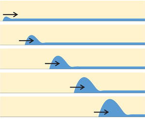
We begin with the classical example of dewetting under adiabatic conditions (in the absence of any overall heat and mass transfer between liquid, solid and ambient gas). Consider a smooth solid substrate initially covered by a thick (at least micrometric) liquid film of viscous fluid. Such a film is metastable under partial wetting conditions because once a dry hole is created in the film (i.e. the CL appears), the dry area will grow spontaneously. The motion is driven by the capillary forces. As the CL expands outwards, the film collects the liquid situated previously on the dried area. Due to the high viscous friction in the thin film, this liquid cannot flow inside the film. It thus forms a growing ridge that situates along the CL. One can take the vertical cross-section that passes through the centre of a dry hole. The problem is then described in two dimensions, as shown in figure 1. Experimental studies have shown that the CL recedes at a constant speed (Brochard-Wyart et al. Reference Brochard-Wyart, Di Meglio, Quere and de Gennes1991; de Gennes et al. Reference de Gennes, Brochard-Wyart and Quéré2004; Edwards et al. Reference Edwards, Ledesma-Aguilar, Newton, Brown and McHale2016). Conversely, the theoretical analysis by Snoeijer & Eggers (Reference Snoeijer and Eggers2010) has shown that the receding speed  $U_{cl}$ should decline very slowly (logarithmically) with time (or with the ridge size
 $w$ that grows with time).
Dewetting ridge receding over a liquid film while the dry area expands.

Previous dewetting studies concern mainly the adiabatic conditions. However, thin film flows are used extensively in industrial applications where the film evaporation/condensation is employed as a highly efficient mean of heat transfer. Applications include such classical cooling devices as falling film chillers or heat pipes. More recently, dewetting was studied in the context of pulsating heat pipes (Nikolayev Reference Nikolayev2021) and bubble growth in boiling (Urbano et al. Reference Urbano, Tanguy, Huber and Colin2018; Bureš & Sato Reference Bureš and Sato2021).
In all these applications, the phase change occurs simultaneously with dewetting; the liquid film is surrounded by the pure vapour of the same fluid. In this work, we continue the line of thought put forward in our previous paper (Zhang & Nikolayev Reference Zhang and Nikolayev2021), where the lubrication approximation was used to describe the thin film flow. The objectives of this work are threefold. The primary aim is to find the numerical solution to the dewetting problem in the presence of liquid film evaporation created by the heated substrate. For this, one needs to discuss first (§ 2.2) the nanoscale effects relevant to the description of CL vicinity, where the evaporation is extreme. As the slope of the liquid–vapour interface increases in the presence of evaporation, the conventional lubrication approach becomes insufficient. We thus develop the generalised lubrication theory suitable for larger interface slopes. Another objective of this paper is to generalise to the case of evaporation the multiscale theory proposed initially by Snoeijer & Eggers (Reference Snoeijer and Eggers2010) for adiabatic dewetting (§ 2.3). The main parameters of the multiscale theory are discussed, and its results are compared to the numerical solution. The dependence of CL receding speed on the heating rate is discussed. Finally, the numerical results are compared to the experiment in § 3.5.
2. Problem formulation
We start with the conventional lubrication equations and then progressively add extra terms to them that lead to the formulation used for the computations.
2.1. Conventional lubrication equations
Consider the dewetting problem shown in figure 1, where the liquid film of thickness  $h_\infty$ is surrounded by the pure vapour of the same substance. Since the vapour density
 $\rho _v$, viscosity and thermal conductivity are all small compared to the liquid, one can apply the ‘one-sided’ formulation where both the vapour-side hydrodynamic stress and the heat flux into the vapour at the interface are neglected in comparison with values on the liquid side. Therefore, the vapour pressure
 $p_v$ is assumed to be spatially homogeneous. The substrate is assumed to be highly conductive and thus isothermal. The wall temperature
 $T_w=T_{sat}+\Delta T$ can differ from
 $T_{sat}=T_{sat}(p_v)$, thus causing the film evaporation or condensation for positive or negative
 $\Delta T$, respectively.
To begin with, one formulates the dewetting problem by using the conventional lubrication theory in two dimensions  $(x,y)$, where the interface is described as
 $y=h(x,t)$. In the frame of reference of the CL that recedes with the speed
 $U_{cl}$, the governing equation reads (Zhang & Nikolayev Reference Zhang and Nikolayev2021)
 \begin{equation} \frac{\partial h}{\partial t} + \frac{\partial}{\partial x} \left( \frac{h^3}{3\mu}\,\frac{\partial \Delta p}{\partial x} - U_{cl} h \right)={-} \frac{J}{\rho_l}, \end{equation}
where  $J$ (assumed positive for evaporation) is the mass flux at the interface, and
 $\mu$ and
 $\rho _l$ are the liquid shear viscosity and density, respectively. In this frame of reference, the transient term
 $\partial h/\partial t$ describes a slow dewetting ridge growth.
A quasi-stationary linear temperature profile is assumed along the  $y$ axis. The interfacial energy balance results in
 \begin{equation} J = \frac{k(T_w-T^i)}{h{\mathcal{L}}}, \end{equation}
where  $T^i$ is the temperature of the vapour–liquid interface,
 $k$ is the liquid heat conductivity, and
 $\mathcal {L}$ is the latent heat.
The pressure jump  $\Delta p\equiv p_v-p_l$ across the vapour–liquid interface satisfies the Laplace equation
 \begin{equation} \Delta p = \sigma K, \end{equation}
where  $\sigma$ is the surface tension, and the interface curvature is
 \begin{equation} K\simeq \frac{\partial^2h}{\partial x^2} \end{equation}
in the small-slope approximation.
2.2. Relaxing the singularity at the contact line
Even for the adiabatic case (i.e. for  $\Delta T = 0$), the conventional hydrodynamic description of the moving CL leads to the viscous dissipation divergence at the CL where
 $h\to 0$ (de Gennes Reference de Gennes1985). Wayner (Reference Wayner1993) was the first to hypothesise that this singularity can be relaxed for volatile fluids through evaporation/condensation when it matches CL displacement. Rather than sliding over the solid, the CL recedes because liquid on it evaporates, or advances by liquid condensation. It turns out to be possible thanks to the Kelvin effect. The Kelvin effect provides the variation of
 $T^i$ along a curved interface:
 \begin{equation} T^i = T_{sat}\left( 1 + \frac{\Delta p}{{\mathcal{L}}\rho_l} \right). \end{equation}
The interface is strongly curved near the CL to agree with the phase change rate, which, in turn, is regulated by CL motion. Within such a description, Janeček & Nikolayev (Reference Janeček and Nikolayev2012) have shown that the liquid pressure remains finite at the CL, thus the singularity is relaxed. Janeček et al. (Reference Janeček, Andreotti, Pražák, Bárta and Nikolayev2013) and Rednikov & Colinet (Reference Rednikov and Colinet2013) have used asymptotic matching to show that the Kelvin effect is sufficient to describe CL motion in case of volatile fluids.
In the diabatic case ( $\Delta T \neq 0$), an additional singularity related to the mass change term
 $J$ appears in (2.1). Indeed, if the Kelvin effect was neglected, then
 $T_w-T^i$ would be constant (
 $=\Delta T$), and the mass flux (2.2) would diverge as
 $h\to 0$. The Kelvin effect relaxes the singularity in this case too. One notes that the singularity relaxation can be achieved even without accounting for the Kelvin effect. The moving CL singularity can be regularised by introducing the hydrodynamic slip at the liquid–solid interface (Hocking Reference Hocking1983). However, accounting for an additional nanoscale effect, the interfacial resistance is necessary to regularise the mass flux (Hocking Reference Hocking1995; Saxton et al. Reference Saxton, Vella, Whiteley and Oliver2017) in the case where it exists – note the correction (Anderson & Janeček Reference Anderson and Janeček2018) of the Hocking formula.
2.2.1. Hydrodynamic slip and interfacial thermal resistance
The no-slip boundary condition at the liquid–solid interface can be violated when the hydrodynamic stress is very strong. The slip length  $l_s$ is introduced to quantify the slip of liquid molecules over the solid;
 $l_s$ is defined as a distance from the liquid–solid boundary where the linear extrapolation of the tangential component of the liquid velocity
 $u_x(y)$ vanishes. Using
 $l_s$, the Navier slip boundary condition is written as
 \begin{equation} u_x = l_s\,\frac{\partial u_x}{\partial y}. \end{equation}
The value of  $l_s$ is usually several nanometres but can be one order of value larger for non-wettable surfaces (Lauga, Brenner & Stone Reference Lauga, Brenner and Stone2007). In all our calculations, we assume
 $l_s=10\,{\rm nm}$, which is the value coherent with the previous works accounting for it (Delon et al. Reference Delon, Fermigier, Snoeijer and Andreotti2008; Nikolayev Reference Nikolayev2010; Janeček & Nikolayev Reference Janeček and Nikolayev2012; Fourgeaud et al. Reference Fourgeaud, Ercolani, Duplat, Gully and Nikolayev2016; Chan et al. Reference Chan, Kamal, Snoeijer, Sprittles and Eggers2020). With the account of the slip, the governing equation (2.1) becomes
 \begin{equation} \frac{\partial h}{\partial t} + \frac{\partial}{\partial x} \left[ \frac{h^2}{3\mu}\,(h +3l_s)\, \frac{\partial \Delta p}{\partial x} - U_{cl} h \right]={-} \frac{J}{\rho_l}. \end{equation}
The interfacial thermal resistance  $R^i$ is of importance when the interfacial mass flux
 $J$ is strong, so the corresponding vapour escape speed is comparable with the thermal velocity of molecules (Nikolayev Reference Nikolayev2022). It is true at the CL where
 $J$ is high. The interfacial thermal resistance reads
 \begin{equation} R^i = \frac{T_{sat} \sqrt{2{\rm \pi} R T_{sat}/M} (\rho_l-\rho_v) }{2 {\mathcal{L}}^2 \rho_l \rho_v }, \end{equation}
where  $R$ is the universal gas constant, and
 $M$ is the molar mass. Here,
 $R^i$ provides an extra term to (2.5):
 \begin{equation} T^i = T_{sat}\left( 1 + \frac{\Delta p}{{\mathcal{L}}\rho_l} \right) + R^i J {\mathcal{L}}, \end{equation}
and (2.2) modified by  $R^i$ and the Kelvin effect reads
 \begin{equation} J=\frac{\Delta T- \Delta p\,T_{sat}/(\rho_l {\mathcal{L}})}{{\mathcal{L}}(R^i +h/k)}. \end{equation}
Without the Kelvin effect, the account of both  $R^i$ and
 $l_s$ provides a finite
 $J$ and a logarithmically divergent
 $p_l$ at the CL. This divergence is integrable, which means that the measurable hydrodynamic stress is finite, so the singularity is relaxed. The introduction of the Kelvin effect leads to a finite pressure at the CL, which is more reasonable from the physical point of view and much more convenient for numerical calculations where a pressure boundary condition can be imposed (see § 2.6) instead of using the numerical matching to asymptotic solutions at
 $x\to 0$ required in the absence of the Kelvin effect.
In order to obtain results comparable to experimental data, one needs to account for two more effects known to considerably affect the free interface shape in the CL vicinity (see § 2.4): the Marangoni effect and vapour recoil.
2.2.2. The Marangoni effect
Since the temperature (2.9) varies along the interface, the corresponding variation of surface tension can be important:
 \begin{equation} \frac{\partial \sigma }{\partial x} \simeq{-} \gamma\,\frac{\partial T^i}{\partial x}, \end{equation}
where  $\gamma =-\partial \sigma /\partial T$ is generally positive for pure fluids. Such a variation contributes to the tangential interface stress component (which is referred to as the Marangoni effect). An extra term should be added to (2.7), which becomes (Nikolayev Reference Nikolayev2010)
 \begin{equation} \frac{\partial h}{\partial t} + \frac{\partial}{\partial x} \left\{\frac{1}{\mu}\left[ \frac{h}{2}\,(h+2l_s )\,\frac{\partial \sigma}{\partial x} +\frac{h^2}{3}\,( h +3l_s )\,\frac{\partial \Delta p}{\partial x}\right] - U_{cl} h \right\}={-} \frac{J}{\rho_l}. \end{equation}
Note that the temperature variation occurs only at the nanoscale; at a larger scale, the interfacial temperature is constant.
2.2.3. Vapour recoil
The recoil pressure  $p_r$ (Nikolayev & Beysens Reference Nikolayev and Beysens1999) is created at the liquid–vapour interface by the fluid molecules escaping the interface towards the vapour. This effect modifies the pressure jump (2.3):
 \begin{equation} \Delta p = \sigma K - p_r, \end{equation}
where
 \begin{equation} p_r = {J^2}\left( \frac{1}{\rho_v} - \frac{1}{\rho_l} \right). \end{equation}
The vapour recoil also affects the interfacial temperature by providing an additional term to (2.9) (Anderson et al. Reference Anderson, Cermelli, Fried, Gurtin and McFadden2007):
 \begin{equation} T^i = T_{sat}\left[ 1 + \frac{\Delta p}{{\mathcal{L}}\rho_l} + \frac{J^2}{2{\mathcal{L}}}\left( \frac{1}{\rho_v^2} - \frac{1}{\rho_l^2} \right) \right] + R^i J {\mathcal{L}} . \end{equation}
Together with (2.2), (2.13) and (2.15), (2.12) governs the interface evolution.
2.3. Multiscale analysis
Equation (2.12) is complex because it involves several very different length scales. Since these scales generally differ by several orders of magnitude, one can apply the multiscale asymptotic analysis. The governing physical effects at one scale can be neglected at another. For the problem of a moving CL with phase change (Janeček et al. Reference Janeček, Andreotti, Pražák, Bárta and Nikolayev2013), three scales (and the corresponding regions) can be identified (figure 2).
Length scale hierarchy in the case of a moving contact line: (a) microscopic region, (b) intermediate region, (c) macroscopic region.

The smallest scale is traditionally referred to as the microregion. Its characteristic size  $\ell _V \sim 100\,{\rm nm}$ is called hereafter the Voinov length. Its rigorous definition will be given below. In figure 2(a), the microregion is illustrated for the partial wetting case with the microscopic contact angle
 $\theta _{micro}$, which is the actual contact angle at the CL. Within this region, phase change is the dominant phenomenon; the nanoscale effects discussed in § 2.2 are all significant. The flow caused by evaporation is so strong that the impact of CL motion is negligible, so both transient and
 $U_{cl}$ terms can be neglected in (2.12). At the right-hand boundary of the microregion (far from the CL), the interface slope saturates to a value that we call hereafter the Voinov angle
 $\theta _V$, which depends on
 $\theta _{micro}$ and
 $\Delta T$ (Janeček & Nikolayev Reference Janeček and Nikolayev2012). Intensive evaporation near the CL induces a strong liquid flow towards it, which, together with the vapour recoil (Nikolayev Reference Nikolayev2022), leads to a strongly curved interface. As a consequence,
 $\theta _V>\theta _{micro}$. The opposite tendency occurs at condensation. In the adiabatic case (
 $\Delta T=0$),
 $\theta _V=\theta _{micro}$.
The intermediate region (typically between  $100\,{\rm nm}$ and
 $100\,{\mathrm {\mu } {\rm m}}$ from the CL) is dominated by the flow induced by CL motion, so the terms responsible for the evaporation-induced flow (and discussed above nanoscale effects) can all be neglected together with the transient term. The interfacial shape is a result of a balance of the surface tension and viscous forces. Such a problem has been investigated by many researchers. Voinov (Reference Voinov1976) has derived an asymptotic law that predicts the interface slope
 $\phi$ as a function of CL velocity:
 \begin{equation} \phi^3 = \theta^3-9\,Ca\ln \frac{x}{\ell_V}, \end{equation}
where the dimensionless dewetting speed (the capillary number) is  $Ca=\mu U_{cl}/\sigma$. It is positive for the CL receding and negative for advancing over the dry area. By considering the corresponding Stokes problem, Cox (Reference Cox1986) showed that its solution can be approximated with (2.16). The approximation remains accurate until a slope as high as
 $150^\circ$ (Snoeijer & Andreotti Reference Snoeijer and Andreotti2013). Two parameters,
 $\ell _V$ and
 $\theta$, should be determined from the asymptotic matching to the microregion solution. As we will see in § 3.2,
 $\theta =\theta _V$.
One of the main objectives of problems involving the CL is to calculate the apparent contact angle  $\theta _{app}$, i.e. the contact angle obtained at the macroscopic scale corresponding to the dewetting ridge size (Snoeijer & Andreotti Reference Snoeijer and Andreotti2013; Nikolayev Reference Nikolayev2022). The corresponding region is often called the macroregion. Such a problem is defined by the balance of the transient and surface tension terms in (2.12). Snoeijer & Eggers (Reference Snoeijer and Eggers2010) considered the adiabatic dewetting problem. They have shown that after initial transients, the macroscopic ridge shape is defined mainly by the surface tension. This means that
 $\theta _{app}$ can be obtained by fitting the ridge shape to a circle (figure 1). With the slip used for the singularity relaxation, Snoeijer & Eggers (Reference Snoeijer and Eggers2010) have performed the asymptotic matching between the CL region, the macroscopic liquid ridge and the flat film of thickness
 $h_\infty$ in the adiabatic case. One of their central results is
 \begin{equation} \theta^3_{app} =\theta^3_V-9\,Ca\ln \frac{2w}{e\ell_V}, \end{equation}
where  $w$ is the ridge half-width (figure 1), and
 $e\simeq 2.71$ is the Euler number. The problem solved by Snoeijer & Eggers (Reference Snoeijer and Eggers2010) is adiabatic; their
 $\ell _V$ is thus equal to
 \begin{equation} \ell_{Vsa}=\frac{3l_s}{e\theta_{micro}}. \end{equation}
The main result of Snoeijer & Eggers (Reference Snoeijer and Eggers2010) is the asymptotic expression for the dewetting speed,
 \begin{equation} Ca=\frac{\theta^3_V}{9}\left[ \ln \left( \frac{4a}{e^2}\,Ca^{1/3}\,\frac{w^2}{\ell_V h_\infty} \right) \right] ^{{-}1}, \end{equation}
where  $a\simeq 1.094$. As argued by Fourgeaud et al. (Reference Fourgeaud, Ercolani, Duplat, Gully and Nikolayev2016), both expressions above should hold for any microregion model (including that accounting for the evaporation) because of the scale separation. However, one needs to determine the key parameters
 $\ell _V$ and
 $\theta _V$, and verify if (2.17) and (2.19) are indeed valid under the conditions of evaporation. To explain their experimental results, Fourgeaud et al. (Reference Fourgeaud, Ercolani, Duplat, Gully and Nikolayev2016) hypothesised that the liquid mass loss caused by strong evaporation at the CL can accelerate the CL receding, in addition to the capillary effect described by (2.19). This issue needs to be clarified.
2.4. Relative contributions of different nanoscale effects
Two main effects that can relax the hydrodynamic CL singularity are the Kelvin effect and the hydrodynamic slip, which together determine  $\ell _V$. The other effects considered above are generally secondary for
 $\ell _V$ but impact
 $\theta _V$ more or less strongly. A contribution of an effect to the overall system dynamics can be evaluated by defining the corresponding characteristic length scales. They are defined as a distance from the CL along the
 $x$ axis at which the effect is still important. An effect overcomes another if its characteristic length is larger. The definitions of these scales presented in table 1 are discussed in Appendix B.
Characteristic length scales of different nanoscale effects.

For estimation purposes, one assumes that the liquid forms a straight wedge with the opening angle  $\theta$. The above analysis shows, however, that the interface slope grows from
 $\theta _{micro}$ to
 $\theta _V$ in the microregion. Therefore, one can define the bounds for the characteristic lengths only by using these two values for
 $\theta$.
For all the fluids, the Kelvin length  $\ell _K$ is smaller than the slip characteristic length scale
 $\ell _s$, which means that the slip controls
 $\ell _V$. As the value of
 $\ell _R$ is comparable to
 $\ell _s$, the interfacial thermal resistance strongly impacts the Voinov angle. This is valid for all the fluids. The vapour recoil is generally weak, which is not surprising accounting for the low
 $\Delta T=5\,{{\rm K}}$ considered in table 1. As its corresponding scale is
 $\ell _r\sim \Delta T^2$, it exercises a much stronger influence at a higher
 $\Delta T$. However, this effect is less important for water than for the other two fluids.
One can see that  $\ell _{MR}$ computed at the CL (i.e. with
 $\theta _{micro}$) can be very large. These large values are, however, only the upper bounds. The impact of the Marangoni effect is extremely strong in the close CL vicinity, but drops very quickly as the slope in the microregion increases towards
 $\theta _V$ at the border of the microregion. This analysis shows that, generally, all of the above nanoscale effects impact CL dynamics, and none of them should be neglected.
2.5. Generalised lubrication theory
As the strongest hydrodynamic stresses occur in the CL vicinity, we consider an example of the curved wedge geometry shown in figure 3(a). Nevertheless, the approach presented hereafter does not lose its generality for any liquid film geometry.
Sketch of (a) the curved interface and (b) the straight liquid wedge, corresponding to the point A.

High interface slopes can occur in the dewetting problem at evaporation that causes  $\theta _V>\theta _{micro}$. When the interface slope
 $\phi$ is larger than
 $\sim 30^{\circ }$, the conventional lubrication equation (2.12), valid for small slopes, is hardly applicable. In this case, one can take advantage of a more accurate approach suggested initially by Boender, Chesters & van der Zanden (Reference Boender, Chesters and van der Zanden1991) and rediscovered more recently by Snoeijer (Reference Snoeijer2006). Instead of operating with the coordinate
 $x$, it uses the parametric interface description in terms of the curvilinear coordinate
 $s$ that runs along it, with
 $s=0$ at the CL. Therefore, the following geometrical relations hold:
 $$\begin{gather} \frac{\partial h}{\partial s}=\sin \phi, \end{gather}$$
 $$\begin{gather}\frac{\partial x}{\partial s}=\cos \phi, \end{gather}$$
where  $\phi$ is the local interface slope. The major convenience of such a parametrisation is that instead of the approximation (2.4), one uses the rigorous geometrical curvature definition
 \begin{equation} K=\frac{\partial\phi}{\partial s}. \end{equation}
Consider an interfacial point A with coordinate  $s$. The approach consists in approximating the tangential pressure gradient
 $\partial p_l/\partial s$ at A (figure 3a) by that created by the flow in a straight liquid wedge, the opening angle of which is
 $\phi$; cf. figure 3(b). In other words, if one introduces the polar radius
 $r$ of the point A defined within the corresponding straight wedge, then this hypothesis reads
 \begin{equation} \frac{\partial p_l}{\partial s}\simeq\frac{\partial p_l}{\partial r}. \end{equation}
Here, the right-hand side is calculated within the straight wedge problem; the upper ray of the straight wedge (to which A belongs) is tangential to the curved interface, meaning  $\partial s=\partial r$.
2.5.1. Generalised moving contact line description
This theory was developed initially to describe the adiabatic moving CL problem (at  $J=0$); it was used in many works – see e.g. Delon et al. (Reference Delon, Fermigier, Snoeijer and Andreotti2008) and Chan et al. (Reference Chan, Srivastava, Marchand, Andreotti, Biferale, Toschi and Snoeijer2013, Reference Chan, Kamal, Snoeijer, Sprittles and Eggers2020). In this case, the pressure gradient is induced by the interface motion (in the reference frame where the wedge is immobile). The Stokes problem (see Appendix A) results in
 \begin{equation} \frac{\partial\Delta p}{\partial s}=\frac{3\mu U_{cl}}{h^2}\,\bar F(\phi), \end{equation}
where the spatial homogeneity of  $p_v$ is assumed and
 \begin{equation} \bar F(\phi)=\frac{2}{3}\,\frac{\sin^3\phi}{\phi-\sin\phi\cos\phi}. \end{equation}
One mentions that  $\bar F(\phi \to 0)=1$, so the generalised theory reduces to the conventional lubrication approach for small slopes as expected.
Another generalisation is required to include the hydrodynamic slip in the model. The analytical solution to the Stokes problem is not known for this case. In previous works (Delon et al. Reference Delon, Fermigier, Snoeijer and Andreotti2008; Chan et al. Reference Chan, Srivastava, Marchand, Andreotti, Biferale, Toschi and Snoeijer2013), the slip length was introduced as in the conventional lubrication equation
 \begin{equation} \frac{\partial\Delta p}{\partial s}=\frac{3\mu U_{cl}}{h(h+cl_s)}\,\bar F(\phi) \end{equation}
with the hypothesis  $c=3$. In a subsequent work (Chan et al. Reference Chan, Kamal, Snoeijer, Sprittles and Eggers2020), the
 $c$ coefficient has been found for the specific problem of adiabatic CL dynamics as a function of
 $\theta _{micro}$:
 $c=3-(9/10)\theta _{micro}^2+o(\theta _{micro}^2)$. However, in general,
 $c$ should depend not on the boundary conditions (
 $\theta _{micro}$ is one of them) but on the local interface slope, so the result of Chan et al. (Reference Chan, Kamal, Snoeijer, Sprittles and Eggers2020) cannot be used here directly. We propose the following phenomenological argument that leads to a similar result. In the conventional lubrication equation, the velocity gradient varies linearly along the vertical axis. However, in a wedge geometry, where the flow lines are usually convergent (or divergent), one can reasonably assume that the velocity gradient varies linearly along an arc (which is actually the case in the straight wedge Stokes problem of Appendix A). The arc centre can be defined locally for each interface point A as an intersection of the tangent to the interface with the wall. The arc radius
 $r$ is the distance from A to the centre (figure 3a), with
 $r$ related to
 $h$ via
 \begin{equation} h=r\sin\phi. \end{equation}
The arc length is  $\zeta =\phi r$ or
 \begin{equation} \zeta=h\phi/\sin\phi. \end{equation}
Instead of (2.25), one can thus write
 \begin{equation} \frac{\partial\Delta p}{\partial s}=\frac{3\mu U_{cl}}{\zeta(\zeta+3l_s)}\,F(\phi), \end{equation}
where
 \begin{equation} F(\phi)=\frac{2\phi^2}{3}\,\frac{\sin{\phi}}{\phi-\sin\phi\cos\phi} \end{equation}
satisfies  $F(\phi \to 0)=1$.
Note that (2.28) is equivalent to (2.25) with  $c=3\sin \phi /\phi =3-(1/2)\phi ^2+o(\phi ^2)$. Since
 $\phi \to \theta _{micro}$ near the CL, this expression is quite close to the above result of Chan et al. (Reference Chan, Kamal, Snoeijer, Sprittles and Eggers2020) but has the advantage of being usable universally. On the basis of the above argument, such a ‘
 $\zeta$-formulation’ will be used hereafter for all other terms.
2.5.2. Generalised description including the phase exchange
Mathieu (Reference Mathieu2003) proposed the generalised description of the phase exchange. His approach is based on its strong localisation near the CL. The Stokes problem (§ A.2) assumes that the mass exchange is modelled by a point source  $\varPhi$ localised at the CL. Here,
 $\varPhi$ is defined as a flux through the arc of the length
 $\zeta$ (figure 3):
 \begin{equation} \varPhi=\int_0^{\phi}r\, u_r \,\mathrm{d}\varphi, \end{equation}
where  $u_r$ is the component of the liquid velocity
 $\boldsymbol u$ assumed to be normal to the arc.
For the  $\partial p_l/\partial s$ definition, this model assumes that the flow along the interface at a point with the coordinate
 $s$ (figure 3a) is provided by a source located at a smaller
 $s$ (i.e. closer to the CL) (Janeček & Nikolayev Reference Janeček and Nikolayev2014). Evidently, when the phase exchange is distributed over the interface,
 $\varPhi =\varPhi (s)$. This assumption results in
 \begin{equation} \frac{\partial\Delta p}{\partial s}=\frac{3\mu \varPhi}{\zeta^2(\zeta+3l_s)}\,G(\phi), \end{equation}
where
 \begin{equation} G(\phi)=\frac{\phi^3}{3}\,\frac{4}{\sin\phi\cos\phi-\phi\cos2\phi} \end{equation}
is the correction factor to the conventional lubrication theory (2.12),  $G(\phi \to 0)=1$. The slip length is introduced here similarly to (2.28).
To include both sources of the liquid flow along the wedge, i.e. CL motion and the phase exchange, one can take advantage of the linearity of the Stokes equations. The total pressure drop is thus a sum
 \begin{equation} \frac{\partial\Delta p}{\partial s}=\frac{3\mu [\varPhi\,G(\phi)+\zeta U_{cl}\,F(\phi)]}{\zeta^2(\zeta+3l_s)} \end{equation}
of the contributions (2.28) and (2.31).
One more assumption concerns the Marangoni term. By using the ‘ $\zeta$-formulation’ for it, one can write in an analogy with (2.12):
 \begin{equation} \mu[\varPhi\,G(\phi)+\zeta U_{cl}\,F(\phi)]=\frac{\zeta}{2}\,( \zeta + 2 l_s )\,\frac{\partial \sigma }{\partial s}+\frac{\zeta^2}{3}\,(\zeta+3l_s)\,\frac{\partial\Delta p}{\partial s}. \end{equation}
Such an ansatz can be justified by the diverging flow in a wedge and by the fact that the Marangoni term is important only in the close vicinity of the CL where the slope remains generally small (of the order of  $\theta _{micro}$) in most cases.
By using the liquid volume conservation,  $\varPhi$ can be expressed via the component
 $u_n=\boldsymbol {u}\boldsymbol {\cdot }\boldsymbol {n}$ of the liquid velocity
 $\boldsymbol u$, which is normal to the vapour–liquid interface (with the vector
 $\boldsymbol n$ directed towards the liquid; see figure 3a):
 \begin{equation} \varPhi=\int_0^s u_n(s)\,\mathrm{d}s. \end{equation}
One can rewrite this expression as
 \begin{equation} u_n=\frac{\partial \varPhi}{\partial s} \end{equation}
and make use of the liquid mass conservation at the interface (Nikolayev Reference Nikolayev2010):
 \begin{equation} J=(u^i-u_n)\rho_l. \end{equation}
Here, the interface velocity projection to  $\boldsymbol n$ is
 \begin{equation} u^i={-}\frac{\partial h}{\partial t}\cos\phi. \end{equation}
By eliminating  $\varPhi$ in (2.36) with (2.34) and injecting it into (2.37) together with (2.38), one finally obtains the generalised counterpart of (2.12):
 \begin{align} \frac{{\partial h }}{{\partial t}}\cos\phi + \frac{\partial }{{\partial s}}\left\{ {\frac{1}{{\mu\, G(\phi )}}\left[ \frac{\zeta}{2}\,( \zeta + 2 l_s )\,\frac{\partial \sigma }{\partial s}+\frac{\zeta^2}{3}\,(\zeta+3l_s)\,\frac{\partial\Delta p}{\partial s} \right] - {U_{cl}}\zeta\, \frac{{F(\phi )}}{{G(\phi )}}} \right\} ={-} \frac{J}{{{\rho_l}}}. \end{align}
Two more equations need to be written to define  $\Delta p$ and
 $J$ that appear in (2.39). The temperature distribution is assumed to be linear along the arc length
 $\zeta$ (figure 3a), as suggested by the rigorous thermal analysis of the straight wedge (Anderson & Davis Reference Anderson and Davis1994). Instead of (2.2), one then obtains
 \begin{equation} J = \frac{k(T_w-T^i)}{\zeta {\mathcal{L}}}, \end{equation}
where the interface temperature is expressed with (2.15). The pressure jump equation
 \begin{equation} \frac{\sigma}{\cos\phi}\,\frac{\partial^2h}{\partial s^2} -\Delta p = {J^2}\left( \frac{1}{\rho_v} - \frac{1}{\rho_l} \right) \end{equation}
2.6. Boundary conditions and contact line receding speed
The problem is solved for  $s\in [0, s_f]$, with
 $s_f$ a point far from the ridge, where the film can be assumed flat. The film flatness condition (zero spatial derivatives and
 $\phi =0$) used in (2.39) results in
 \begin{equation} h_\infty=h_0\sqrt{1-\frac{t}{t_d}}, \end{equation}
where  $h_0$ is the initial (
 $t=0$) film thickness, and
 \begin{equation} t_d=\frac{{\mathcal{L}}\rho_l h_0^2}{2k\,\Delta T} \end{equation}
is the film drying time. For the adiabatic problem ( $\Delta T=0$), the thickness
 $h_\infty =h_0$ remains constant.
At the CL ( $s=0$), the geometry implies
 \begin{equation} \left. \begin{aligned} h & = 0, \\ \frac{{\partial h }}{\partial s} & = \sin\theta_{micro}. \end{aligned} \right\} \end{equation}
The set of lubrication equations (2.39) and (2.41) is of fourth order, so one more boundary condition is required. It should express the regularity of all physical quantities at the CL (their finiteness and continuity). To derive this condition for the generalised lubrication approach, one can proceed similarly to Janeček & Nikolayev (Reference Janeček and Nikolayev2012), who obtained it for the conventional case. The temperature continuity implies that the interface temperature  $T^i$ at the CL should be equal to the temperature of the solid,
 $T_w=T_{sat}+\Delta T$. From (2.15), one obtains the condition
 \begin{equation} \Delta p=\frac{{\mathcal{L}}\rho_l}{T_{sat}}\,(\Delta T-R^iJ{\mathcal{L}})-\frac{J^2\rho_l}{2}\left(\frac{1}{\rho_v^2}-\frac{1}{\rho_l^2}\right), \end{equation}
valid asymptotically as  $s\to 0$. To obtain
 $J(s\to 0)$, (2.39) is integrated from 0 to
 $s$, where
 $s$ is infinitesimally small, so
 $\zeta =s\theta _{micro}$. The regularity of all physical quantities results in
 \begin{equation} -\gamma\,\frac{\partial T^i}{\partial s}+\theta_{micro} s\,\frac{\partial\Delta p}{\partial s}=\frac{\mu}{l_s\theta_{micro}} \left[\theta_{micro} U_{cl}\,F(\theta_{micro})-\frac{J\,G(\theta_{micro})}{\rho_l}\right]. \end{equation}
The  $T^i$ derivative can be obtained from (2.40) by developing
 $T^i$ into the Taylor series around
 $s=0$:
 \begin{equation} \frac{\partial T^i}{\partial s}={-}\frac{{\mathcal{L}}\theta_{micro}}{k}\,J. \end{equation}
Its substitution into (2.46) results in the expression
 \begin{equation} s\,\frac{\partial \Delta p}{\partial s}=\frac{\mu}{l_s\theta_{micro}} \left[U_{cl}\,F(\theta_{micro})-J\left(\frac{G(\theta_{micro})}{\theta_{micro} \rho_l}+\frac{l_s{\mathcal{L}}\theta_{micro}}{\mu k}\,\gamma\right)\right]. \end{equation}
By combining (2.45) and (2.48), one obtains a differential equation for  $\Delta p$ that is valid asymptotically. Its solution (Janeček & Nikolayev Reference Janeček and Nikolayev2012) shows that both
 $\Delta p$ and
 $J$ remain finite at the CL. The left-hand side of (2.48) thus tends to zero as
 $s\to 0$, which results in
 \begin{equation} J(s\to 0)=\frac{U_{cl}\,F(\theta_{micro})}{\dfrac{G(\theta_{micro})}{\theta_{micro}\rho_l}+\dfrac{l_s{\mathcal{L}}\theta_{micro}}{\mu k}\,\gamma}. \end{equation}
The pressure value at the CL is obtained easily by substituting (2.49) into (2.45). One can see that the pressure and mass flux are finite at the CL. However, a weaker form of the fourth boundary condition
 \begin{equation} \left. \frac{{\partial \Delta p}}{\partial s} \right|_{s \to 0}= 0 \end{equation}
is more convenient (Zhang & Nikolayev Reference Zhang and Nikolayev2021) to provide a better numerical stability.
Another equation is needed to determine the CL speed (which is a part of the problem); (2.49) can be used for this purpose.
3. Results and discussion
The problem is solved numerically using the finite volume method (in this one-dimensional case, a finite volume is simply a line segment), which provides a better numerical stability than the conventional finite difference method. The numerical algorithm is similar to that used by Nikolayev (Reference Nikolayev2010) and Zhang & Nikolayev (Reference Zhang and Nikolayev2021). The variables and their even-order derivatives are defined at the mesh nodes (the centres of segments), while the odd-order derivatives are defined at the segment boundaries. In order to capture the nanoscale effects without increasing significantly the total number of nodes, the meshing is exponentially refined near the CL. The nonlinear terms are managed with iterations.
The numerical approach is first tested for the adiabatic case against the asymptotic theory of Snoeijer & Eggers (Reference Snoeijer and Eggers2010). We then analyse the dewetting dynamics in the presence of liquid film evaporation. The numerical results are finally compared with the experimental data of Fourgeaud et al. (Reference Fourgeaud, Ercolani, Duplat, Gully and Nikolayev2016).
3.1. Adiabatic dewetting
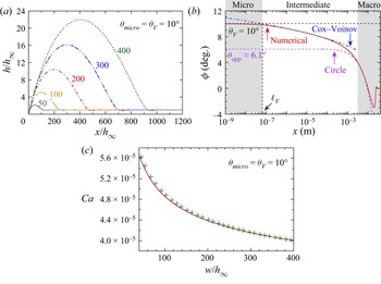
A typical numerical result demonstrating the growth of the dewetting ridge under classical adiabatic conditions ( $\Delta T=0$) is shown in figure 4(a) for
 $\theta _{micro}=10^{\circ }$ and for FC72 (more precisely, n-perfluorohexane) fluid, whose properties are listed in table 2. The flat part of the liquid film has constant thickness
 $h_\infty =50\,{\mathrm {\mu } \textrm {m}}$, which is a typical film thickness in the pulsating heat pipes (Nikolayev Reference Nikolayev2021). The moving CL has been chosen as the frame of reference. Therefore, the CL stays at the origin. The ridge half-width
 $w$ grows with time (see the supplementary movie available at https://doi.org/10.1017/jfm.2022.725), so the evolution is discussed in terms of
 $w$ rather than time to enable a comparison with the multiscale theory.
Numerical results concerning the adiabatic dewetting ( $\Delta T=0$) for
 $\theta _{micro}=10^{\circ }$ and
 $h_\infty =50\,{\mathrm {\mu } \textrm {m}}$. (a) Growth of the liquid ridge (see the supplementary movie). The curve parameter is
 $w/h_\infty$. (b) Interface slope for
 $w/h_\infty =200$. (c) Contact line receding speed
 $Ca$ as a function of the ridge width. Line indicates numerical result; crosses come from (2.19).

Liquid properties at the selected saturation points.

The numerically obtained spatial variation of the interface slope  $\phi$ is shown in figure 4(b) for the time moment at which
 $w/h_\infty =200$ and
 $Ca=4.39\times 10^{-5}$ (red solid line). All three scales discussed in § 2.3 can be recognised.
The intermediate region obeys the governing equation (2.23). Its solution is known to be well approximated by the Cox–Voinov law (2.16). Since the (2.23) is of second order with respect to  $\phi$, its solution contains two integration constants:
 $\theta$ and
 $\ell _V$. Obviously, in the absence of CL motion, the interface is straight, so
 $\phi (Ca=0)=\theta _{micro}$, which results in
 $\theta =\theta _{micro}$. From the definition of the Voinov angle,
 $\theta _V=\theta _{micro}$ for the adiabatic case, and it remains nearly constant in a region that can be identified with the microregion.
The value  $\ell _V\simeq 64\,\textrm {nm}$ is determined from fitting (2.16) to the numerical curve as an abscissa of the intersection of the fitting curve with the horizontal line
 $\phi =\theta _{micro}$. In agreement with the hypothesis of Fourgeaud et al. (Reference Fourgeaud, Ercolani, Duplat, Gully and Nikolayev2016), the
 $\ell _V$ value coincides with that given by the hydrodynamic slip: (2.18) results in
 $\ell _{Vsa}\simeq 63\,\textrm {nm}$. This is not surprising as it exceeds the value provided by the Kelvin effect:
 $\ell _{VK}\simeq 38\,\textrm {nm}$ according to (3.2). This conclusion conforms to the discussion in § 2.4. One needs to note that during the ridge evolution,
 $\ell _V$ grows slightly with
 $w/h_\infty$ (i.e. decreases with
 $Ca$), but the variation is below 3 %. This means that the Cox–Voinov formula is fairly accurate and is thus suitable for multiscale modelling.
As mentioned above, the liquid ridge is of circular shape in the macroregion. The corresponding fit is also plotted in figure 4(b) (violet dashed line). The angle at which this circle intersects the solid surface (i.e. the intersection of the fitting curve with the ordinate axis) defines the apparent contact angle  $\theta _{app}\simeq 6.1^\circ$. The half-width
 $w$ of the ridge can be obtained easily from the fit as a distance between the apparent CL and the ridge summit (figure 1).
The CL receding speed is not rigorously constant but decreases slowly. By using  $w$ and
 $\ell _V$, both obtained from the numerical curve as discussed above, one can compare the numerical
 $Ca$ to the asymptotic result (2.19) (figure 4c). The agreement is excellent, which shows the validity of the approach that we use.
3.2. Dewetting at evaporation
This subsection considers the liquid film evaporation caused by substrate heating. Three different fluids common for heat transfer applications are used in the calculations, whose properties are summarised in table 2. Initially, the liquid film has the thickness  $h_0=50\,{\mathrm {\mu } \textrm {m}}$ typical for the pulsating heat pipe used by Fourgeaud et al. (Reference Fourgeaud, Ercolani, Duplat, Gully and Nikolayev2016) in their experiments.
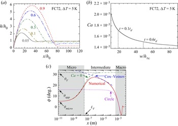
Similarly to the adiabatic case, figure 5(a) demonstrates the dewetting ridge evolution at evaporation. The fluid is FC72 with  $\theta _{micro}=5^{\circ }$, and the substrate superheating is
 $\Delta T=5$ K. Because of evaporation, liquid film thinning occurs, which is clearly visible in the flat film portion. The receding speed
 $Ca$ decreases with time. It is shown in figure 5(b) as a function of the ridge half-width
 $w$ (that increases with time similarly to the adiabatic case).
Numerical results showing the formation of a dewetting ridge for FC72;  $\Delta T=5$ K,
 $\theta _{micro}=5^{\circ }$ and
 $h_0=50\,{\mathrm {\mu } \textrm {m}}$. (a) Growth of the liquid ridge. The curve parameter is
 $t/ t_d$. (b) Evolution of the contact line receding speed
 $Ca$. (c) Interface slope variation for
 $Ca=1.614\times 10^{-3}$.

The central question of the dewetting theory concerns CL dynamics, i.e.  $Ca$ as a function of
 $\Delta T$. However, during the film evolution,
 $Ca$ decreases with time as shown in figure 5(b). For applications (e.g. in pulsating heat pipe modelling), one usually needs only an average speed. As the time evolution is slow,
 $Ca$ can be averaged over a time interval; such an averaging is denoted hereafter with angle brackets. A practical averaging time interval needs to be chosen. Evidently, the averaging makes little sense for times close to
 $t_d$, near which the film evaporates completely. We choose the upper averaging limit to be
 $0.6 t_d$. The averaging needs to be started at a time moment where the influence of initial conditions fades out;
 $0.1 t_d$ is selected as the lower averaging limit. For the case of figure 5(b),
 $\langle Ca\rangle \simeq 1.60\times 10^{-3}$. Repeating the process for different
 $\Delta T$ ranging from 0 to 20 K, we plot
 $\langle Ca\rangle$ as a function of
 $\Delta T$ in figure 6 (as characters with error bars) for several typical
 $\theta _{micro}$ values and for selected fluids. The upper and lower bounds of the error bars correspond to the numerical
 $Ca$ at
 $t=0.1 t_d$ and
 $0.6 t_d$, respectively. The error bars are narrower for small
 $\theta _{micro}$ and
 $\Delta T$, because the speed variation is less drastic.
Comparison of numerical (characters with error bars) and theoretical (lines) results for  $Ca(\Delta T)$ for several
 $\theta _{micro}$ and different fluids.

Note that the dewetting is not only accelerated by the evaporation; it can also be induced by evaporation (Fourgeaud et al. Reference Fourgeaud, Ercolani, Duplat, Gully and Nikolayev2016). This is seen clearly in figure 6. For small  $\theta _{micro}$ (i.e. for conditions of almost complete wetting), the adiabatic dewetting speed is extremely low, which means no dewetting in practice. However, it grows considerably with superheating.
3.3. Comparison to multiscale theory
A full numerical solution of the dewetting problem is, however, time- and resource-consuming because of the necessity to resolve several very different length scales on the one hand, and to iterate to find CL speed at each time moment, on the other. For this reason, the multiscale approach to this problem can be a viable alternative. Let us compare the numerical result and the solutions computed in each of the regions within the multiscale approach to determine if it holds.
Figure 5(c) shows the spatial variation of the interface slope at the time moment  $t=0.33 t_d$. Note the extent of the solution over multiple decades, which it was possible to compute thanks to the mesh refinement near the CL. Similarly to the adiabatic case, three regions can be identified clearly. First, we perform the numerical matching of the microscopic and intermediate regions.
As discussed in § 2.3, the microregion-governing equation can be obtained by neglecting both the transient and the  $U_{cl}$-containing terms in (2.39), which thus reduces to (Janeček & Nikolayev Reference Janeček and Nikolayev2014)
 \begin{equation} \frac{\partial }{{\partial s}}\left\{ \frac{1}{{\mu\,G(\phi )}}\left[ \frac{\zeta}{2}\,( \zeta + 2 l_s )\,\frac{\partial \sigma }{\partial s}+\frac{\zeta^2}{3}\,(\zeta+3l_s)\,\frac{\partial\Delta p}{\partial s} \right]\right\} ={-} \frac{J}{{{\rho_l}}}. \end{equation}
This corresponds to the problem of an evaporating immobile liquid wedge sketched in figure 2(a). The boundary condition  $K=0$ is applied at the right-hand end of the integration interval (which corresponds to the constant slope at infinity) instead of (2.42). The other three boundary conditions (see (2.44) and (2.50)) are defined at the CL and thus remain valid.
The slope variation corresponding to the microregion solution is shown in figure 5(c) (green dash-dotted line). It exhibits the  $\phi$ saturation at large
 $x$ to the value
 $\theta _V\simeq 31.65^{\circ }$. The abscissa axis is extended to non-physically small values to show the
 $x\to 0$ convergence to
 $\theta _{micro}$.
The treatment of the intermediate and macroscopic regions is similar to the adiabatic case considered in § 3.1. The fit (blue dashed line in figure 5c) to the Cox–Voinov law (2.16) with  $\theta =\theta _V$ results in
 $\ell _V\simeq 20\,\textrm {nm}$ for this particular case. The fit to a circle in the macroregion (violet dotted line in figure 5c) gives
 $\theta _{app}\simeq 15.7^\circ$.
By repeating the fitting for different  $\Delta T$ ranging from 0 to 20 K and for three selected fluids, one obtains figure 7, which demonstrates
 $\theta _V$ and
 $\langle \theta _{app}\rangle$ as functions of
 $\Delta T$ for different fluids. As
 $\theta _{app}$ increases slowly with time as the ridge grows, an average value
 $\langle \theta _{app}\rangle$ is taken over the course
 $(0.1t_d,0.6t_d)$. Here,
 $\theta _V$ increases monotonically with
 $\Delta T$ as discussed in numerous works on the microregion (see Nikolayev (Reference Nikolayev2022) for a review);
 $\theta _V(\Delta T=0)=\theta _{micro}$.
Values of  $\theta _V$ (red diamonds) and
 $\langle \theta _{app}\rangle$ (blue crosses) as functions of
 $\Delta T$ for different fluids. The numerical data are shown with characters, while the blue dotted line corresponds to the multiscale theory result for
 $\langle \theta _{app}\rangle$.

The Voinov length  $\ell _V$ obtained from the Cox–Voinov fit depends on time but its variation is extremely weak, of the order of the fitting error (less than 2 %). We plot
 $\ell _V$ as a function of
 $\Delta T$ in figure 8 for different fluids. As expected for the microregion scale,
 $\ell _V$ is of the order of 10–100 nm. It shrinks monotonically with
 $\Delta T$.
Numerically obtained variation of  $\ell _V$ with
 $\Delta T$ (lines) for different fluids. The variations of
 $\ell _{VK}$ (diamonds) and
 $\ell _{Vs}$ (crosses) are also shown. The value of
 $\ell _{Vsa}$ from (2.18) corresponds to
 $\ell _{Vs}(\Delta T=0)$.

One can now use the multiscale theoretical prediction (2.17) to compare with the numerical data. The averaged values of all parameters obtained from the numerical calculation (such as  $\langle w\rangle$ and
 $\langle Ca\rangle$) can be used on the right-hand side of (2.17). The resulting
 $\langle \theta _{app}\rangle$ is plotted as a function of
 $\Delta T$ as blue dotted lines for different fluids in figure 7. A good agreement with the numerical data for all the fluids indicates the success of the multiscale theory.
More importantly, it is possible to compare the numerics to the asymptotic theoretical result (2.19) for  $\langle Ca\rangle$. The averaged values of all the parameters
 $\langle w\rangle$,
 $\langle h\rangle$,
 $\theta _V$ and
 $\ell _V$ obtained from the numerical calculation can be used in the right-hand side of (2.19). In figure 6, the lines show the theoretical results while the characters are the numerical data. Again, the agreement is excellent. One concludes that the multiscale theory is valid for the evaporation case.
3.4. Voinov length approximation
Two key parameters engendering from the microregion enter (2.19):  $\theta _V$ and
 $\ell _V$. While the first parameter
 $\theta _V$ of the multiscale theory is relatively easy to obtain as it requires solving only the microregion problem, the second parameter
 $\ell _V$ is a more delicate issue. To avoid the laborious numerical calculation of
 $\ell _V$ for a particular fluid and
 $\Delta T$, a simpler approach is desirable.
In the case of phase change, if only the Kelvin effect is included, then one finds a general expression for the Voinov length (Janeček et al. Reference Janeček, Andreotti, Pražák, Bárta and Nikolayev2013)
 \begin{equation} \ell_{VK}\simeq f(\epsilon)\,\frac{\sqrt{3\mu k T_{sat}}}{\theta_V^2 \rho_l \mathcal{L}}, \end{equation}
where
 \begin{equation} \epsilon=\frac{\sqrt{3 \mu k T_{sat}}}{\sigma \theta_V^3}\,\frac{\Delta T}{T_{sat}}, \end{equation}
and  $f(\epsilon )$ is an increasing function shown in figure 3(b) of Janeček et al. (Reference Janeček, Andreotti, Pražák, Bárta and Nikolayev2013); for positive
 $\Delta T$, it varies between
 $f(0)\simeq 1.31$ and
 $f(\epsilon _c)\simeq 3.02$. Note that for large
 $\Delta T$,
 $\epsilon$ tends to a critical value
 $\epsilon _c\simeq 0.3$, which results in
 $\theta _V\sim \Delta T^{1/3}$.
However, because other nanoscale effects have been accounted for in the calculation, figure 8 shows that, at least for conventional fluids, this value  $\ell _{VK}$ remains much smaller than the numerical result and is thus hardly suitable in practice.
The slip-controlled value  $\ell _{Vsa}$ (2.18) that was used by Fourgeaud et al. (Reference Fourgeaud, Ercolani, Duplat, Gully and Nikolayev2016) for
 $\ell _{V}$ is known only for
 $\Delta T=0$. Its value can be somewhat larger than the numerical
 $\ell _V$ for
 $\Delta T\neq 0$ (figure 8), so one needs a better general expression. On the basis of the scaling discussed in § 2.4, the slip should have a major impact on
 $\ell _V$. Therefore, we propose to use for
 $\ell _V$ the expression
 \begin{equation} \ell_{Vs}=\frac{3l_s}{e\theta_V}. \end{equation}
Figure 8 shows that the quality of this approximation is satisfactory, especially accounting for the fact that  $\ell _V$ always appears under the logarithm in (2.17) and (2.19).
3.5. Comparison with experiment
The only experiment on the dewetting at evaporation, which comprises the data on both  $\theta _{app}$ and
 $Ca$, and with which we can thus compare our modelling, was conducted by Fourgeaud et al. (Reference Fourgeaud, Ercolani, Duplat, Gully and Nikolayev2016). They have observed the dewetting of an ethanol film on a heated sapphire substrate, in an airtight chamber filled with the saturated ethanol vapour. Initially, an ethanol film of thickness
 $\sim 60\,{\mathrm {\mu } \textrm {m}}$ was deposited on the solid surface, whose temperature was above the saturation temperature of the vapour. Both substrate dewetting and liquid film thinning were observed. The time evolution of the interface profile (including CL position,
 $w$ and
 $h_\infty$) and the vapour pressure were recorded. Hence CL speed could be derived. Here,
 $T_{sat}$ was found with the vapour pressure. The value of
 $\theta _{app}$ was obtained by fitting the liquid ridge profile to a circle, whose intersection with the solid surface gave
 $\theta _{app}$, similarly to our numerical procedure. The substrate temperature
 $T_w$ could not be measured, but it was clear that it remained nearly constant because of the large thermal inertia of the substrate. The superheating
 $\Delta T=T_w-T_{sat}$ varied because of strong
 $T_{sat}$ variation. According to the assumption of Fourgeaud et al. (Reference Fourgeaud, Ercolani, Duplat, Gully and Nikolayev2016),
 $T_w=48^\circ$C. In the present work, we propose another approach. Instead of assuming a
 $T_w$ value, we calculate
 $\Delta T$ for each data point from the experimental
 $Ca$ by using the numerical
 $Ca(\Delta T)$ curve for ethanol (figure 6c). The calculation is done for
 $\theta _{micro}=5^{\circ }$, which is the value found originally by Fourgeaud et al. (Reference Fourgeaud, Ercolani, Duplat, Gully and Nikolayev2016).
Figure 9(a) plots the experimental data for  $Ca(t)$ (green squares) and the numerical curve
 $Ca(\Delta T)$ (blue solid line, the same as in figure 6c). By placing the experimental
 $Ca$ value to the numerical curve, one recovers
 $\Delta T$ for each experimental point. For instance, for the first data point at
 $t=0.375\,{\textrm {s}}$, given
 $Ca\simeq 1.57\times 10^{-3}$, one recovers
 $\Delta T\simeq 8.9\,\textrm {K}$.
(a) Experimental data of Fourgeaud et al. (Reference Fourgeaud, Ercolani, Duplat, Gully and Nikolayev2016) for  $Ca(t)$ (green squares plotted with respect to the lower abscissa axis) and numerical curve
 $Ca(\Delta T)$ (blue line plotted with respect to the upper abscissa axis). (b) Comparison of
 $\theta _V(\Delta T)$ functions obtained with the experimental data (Fourgeaud et al. Reference Fourgeaud, Ercolani, Duplat, Gully and Nikolayev2016) (red diamonds) and the numerical calculation (line).

In the next step,  $\ell _V$ can be computed from the numerical curve
 $\ell _V(\Delta T)$ (figure 8c). Finally, one can calculate
 $\theta _V$ with (2.17) by using the experimental data for
 $\theta _{app}$ and
 $w$ and the
 $\ell _V$ found before. We note that the latter has only a small impact on the result as it enters under the logarithm. The points
 $(\Delta T,\theta _V)$ obtained in this way are plotted in figure 9(b) as red diamonds. As demonstrated in figure 7,
 $\theta _V$ can also be obtained numerically as a function of
 $\Delta T$. The corresponding dependence is plotted as the red curve in figure 9(b), the same as the diamonds in figure 7(c). The numerical line agrees with the experimental estimations, which shows the validity of our numerical approach.
We should also verify that  $T_w=T_{sat}+\Delta T$ remains nearly constant for all data points. From our
 $\Delta T$ evaluation,
 $T_w=42.7\pm 0.4\,^\circ$C. Such a value is a plausible estimation of
 $T_w$. In their original work, Fourgeaud et al. (Reference Fourgeaud, Ercolani, Duplat, Gully and Nikolayev2016) obtained a difference of
 $\simeq 14$% between the theoretical and experimental
 $Ca$ values. We can see now that this difference can be attributed to their overestimation of
 $T_w$.
4. Conclusions
The dewetting dynamics in the presence of the liquid film evaporation is analysed for the case where the liquid film is in contact with the pure vapour of the same fluid. To increase the precision of numerical results at an interface slope higher than the conventional lubrication theory can handle, we develop the generalised lubrication theory (which uses, however, phenomenological arguments yet to be verified). Several nanoscale effects are included to produce realistic results: hydrodynamic slip, interfacial thermal resistance, Kelvin and Marangoni effects, and the vapour recoil. The relative importance of all these effects is analysed. Our scaling analysis shows that, in general, none of the above nanoscale effects should be neglected while evaluating the evaporation impact. The Kelvin effect, while being less important in terms of its magnitude, is needed to provide the finiteness of liquid pressure at the contact line. Our theoretical description leads to the contact line receding phenomenon accompanied by the spontaneous liquid evaporation in its close vicinity. The evaporation rate at the contact line conforms to its speed. In the presence of the forced evaporation caused by substrate heating, the dewetting accelerates. The results show that the dewetting phenomenon is not only accelerated at evaporation; the dewetting can also be induced by evaporation. The dependence of the dewetting speed on the substrate superheating has been computed for three fluids (FC72, ethanol and water) for different wetting conditions. Unfortunately, it is difficult at this stage to introduce an analytical theory showing the importance of the boosting effect of evaporation because of a large number of effects that contribute to it.
The model has been validated against the asymptotic multiscale theory of dewetting developed by Snoeijer & Eggers (Reference Snoeijer and Eggers2010) for adiabatic conditions. The multiscale theory has been generalised to the evaporation case. It results in a simple analytical expression for the dewetting speed. The main parameters of this expression are the Voinov length and the Voinov angle (the interface slope formed in the microregion), through which the nanoscale effects impact the macroscale physics. While the Voinov angle is relatively easy to compute (it requires only a solution of a stationary microregion model mastered by many research groups), the Voinov length requires a more sophisticated calculation. An approximate analytical formula for the Voinov length is proposed. The results of the generalised multiscale model agree with the numerical calculations. It is shown that the evaporative mass loss at the contact line (hypothesised by Fourgeaud et al. Reference Fourgeaud, Ercolani, Duplat, Gully and Nikolayev2016) does not lead to any additional acceleration of its motion controlled entirely by capillarity and by the evaporation-driven modification of the Voinov angle.
The numerical results have been compared to the experiment of Fourgeaud et al. (Reference Fourgeaud, Ercolani, Duplat, Gully and Nikolayev2016). For this, their experimental data were reanalysed, and good agreement with our numerics was achieved.
This study's results are of importance for many applications such as bubble growth in boiling (in particular, the microlayer dynamics; Tecchio et al. Reference Tecchio, Zhang, Cariteau, Zalczer, Roca i Cabarrocas, Bulkin, Charliac, Vassant and Nikolayev2022) and pulsating heat pipes, where the liquid film dynamics crucially affects the overall heat exchange.
Supplementary movie
A supplementary movie is available at https://doi.org/10.1017/jfm.2022.725.
Funding
The present work is supported by the project TOPDESS, financed through the Microgravity Application Programme by the European Space Agency. This paper is also a part of the PhD thesis of X.Z. co-financed by the CNES and the CEA NUMERICS programme, which has received funding from the European Union Horizon 2020 research and innovation programme under the Marie Skłodowska-Curie grant agreement no. 800945. Additional financial support of CNES awarded through GdR MFA is acknowledged.
Declaration of interests
The authors report no conflict of interest.
Appendix A. Stokes problems in the straight wedge
In the polar reference  $(r,\varphi )$ (figure 3b), the components of the liquid velocity
 $\boldsymbol u=(u_r, u_\varphi )$ can be expressed as
 \begin{equation} \left. \begin{aligned} u_r & =\frac{1}{r}\,\frac{\partial\varPsi}{\partial\varphi}, \\ u_\varphi & ={-}\frac{\partial\varPsi}{\partial r}. \end{aligned} \right\} \end{equation}
with the stream function  $\varPsi$ that satisfies the equation
 \begin{equation} \nabla^4\varPsi=0. \end{equation}
Because of the mass conservation along the wedge in both problems considered below, the liquid flux  $\varPhi$ defined by (2.30) is independent of
 $r$.
A.1. Liquid flow created by contact line motion
Consider the substrate moving with speed  $U_{cl}$ to the left in figure 3(b), which is equivalent to the CL receding. The boundary conditions to (A2) are
 \begin{equation} \left. \begin{aligned} \frac{\partial\varPsi}{\partial\varphi} & ={-}r U_{cl} \quad \textrm{and}\quad \frac{\partial\varPsi}{\partial r}=0\quad \textrm{at } \varphi=0,\\ \frac{\partial\varPsi}{\partial r} & =0\quad \textrm{and}\quad \frac{\partial^2\varPsi}{\partial\varphi^2}=0\quad \textrm{at }\varphi=\phi. \end{aligned} \right\} \end{equation}
The solution to this problem is (Moffatt Reference Moffatt1964)
 \begin{equation} \varPsi(r,\varphi)={-}r U_{cl}\,\frac{(2\phi-\varphi) \sin\varphi-\varphi\sin(2\phi-\varphi)}{2\phi-\sin(2\phi)}, \end{equation}
and the pressure gradient at the interface reads
 \begin{equation} \frac{\partial p_l}{\partial r}=U_{cl}\,\frac{\mu}{r^2}\,\frac{4\sin\phi}{\sin(2\phi)-2\phi}, \end{equation}
which is equivalent to (2.23) accounting for (2.26).
Note that  $\varPhi =0$ for this case as it is zero in the apex. Many authors pointed out the non-integrable pressure divergence
 $p\sim r^{-2}$. This means the infinite viscous dissipation, so such a problem statement is in fact non-physical, and other microscale phenomena like the hydrodynamic slip and/or the Kelvin effect need to be accounted for to relax the singularity.
A.2. Liquid flow created by localised evaporation
Consider the flow induced by a the localised evaporation modelled by a point source  $\varPhi$ placed at the wedge apex (figure 3b). The boundary conditions to (A2) are
 \begin{equation} \left. \begin{aligned} \frac{\partial\varPsi}{\partial\varphi} & =0 \quad \textrm{and}\quad \frac{\partial\varPsi}{\partial r}=0\quad \mathrm{at}\ \varphi=0,\\ \frac{\partial\varPsi}{\partial r} & =0\quad \textrm{and}\quad \frac{\partial^2\varPsi}{\partial\varphi^2}=0\quad\textrm{at }\varphi=\phi. \end{aligned} \right\} \end{equation}
They signify (i) the impermeability and no-slip conditions at the solid surface  $\varphi =0$, and (ii) the impermeability and zero tangential stress at the liquid–vapour interface
 $\varphi =\phi$. The velocity should satisfy (2.30), where
 $\varPhi$ is constant. One mentions that for this,
 $\varPsi (r,\varphi )$ should be independent of
 $r$.
The solution found by Mathieu (Reference Mathieu2003) is
 \begin{equation} \varPsi(r,\varphi)=\varPhi\,\frac{\sin(2\phi-2\varphi)+2\varphi\cos(2\phi)}{2\phi \cos(2\phi)-\sin(2\phi)}. \end{equation}
The corresponding pressure field is
 \begin{equation} p_l(r,\varphi)=\varPhi\,\frac{\mu}{r^2}\,\frac{4\cos(2\phi-2\varphi)}{\sin(2\phi)-2\phi \cos(2\phi)}, \end{equation}
and the pressure gradient at the interface  $\varphi =\phi$ reads
 \begin{equation} \frac{\partial p_l}{\partial r}=\varPhi\,\frac{\mu}{r^3}\,\frac{4}{\phi \cos(2\phi)-\cos{\phi}\sin{\phi}}, \end{equation}
which is equivalent to (2.31) with  $l_s=0$.
Appendix B. Characteristic length scales in the microregion
The characteristic lengths shown in table 1 can be obtained from (2.13)–(2.15) and (3.1) describing the microregion. For these estimations, small slopes are assumed, so  $G\simeq 1$ and
 $\zeta \simeq h$. One assumes for the estimation the wedge liquid shape with the opening angle
 $\theta$. Therefore, if one denotes the
 $x$ scale as
 $\ell$ (to be defined for each effect), then the
 $h$ scale is
 $\theta \ell$. One finds from (2.4) that
 $K\sim \theta /\ell$, so
 $\Delta p\sim \sigma K\sim \sigma \theta /\ell$. The mass flux scales as
 $J\sim k\,\Delta T/({\mathcal {L}}\theta \ell )$. From (2.10), one finds the interfacial resistance scale
 $\ell _R=R^ik/\theta$. From (2.13), one finds the vapour recoil scale
 $\ell _r$. It reflects the vapour recoil on the Voinov angle. The slip length scale
 $\ell _s$ is easily found from (3.1). The Kelvin length scale
 $\ell _K$ is derived by Janeček et al. (Reference Janeček, Andreotti, Pražák, Bárta and Nikolayev2013).
The Marangoni effect is more delicate because the  $T^i$ spatial variation does not appear without either Kelvin or interface resistance terms; cf. (2.9). After having left aside the slip, (3.1) reduces to
 \begin{equation} \frac{1}{\mu}\,\frac{\partial}{\partial x}\left[-\frac{\gamma h^2}{2}\,R^i{\mathcal{L}}\,\frac{\partial J}{\partial x} + \left(\frac{h^3}{3} - \frac{\gamma h^2}{2}\,\frac{T_{sat}}{{\mathcal{L}}\rho_l} \right)\frac{\partial\Delta p}{\partial x}\right] ={-} \frac{J}{\rho_l}. \end{equation}
By comparing the two terms in the round brackets (the second of which comes from the Kelvin effect), one obtains the Marangoni–Kelvin scale
 \begin{equation} \ell_{MK}=\dfrac{3\gamma T_{sat}}{2\theta{\mathcal{L}}\rho_l}. \end{equation}
It appears to be below  $1\,\textrm {nm}$ for all the cases under consideration, so the corresponding effect is negligible. Conversely, the Marangoni effect appearing due to the interfacial thermal resistance with respect to the capillary action is characterised by the balance of the terms
 \begin{equation} \frac{\gamma h^2}{2}\,R^i{\mathcal{L}}\,\frac{\partial J}{\partial x}\quad \textrm{and}\quad \frac{h^3}{3}\, \frac{\partial\Delta p}{\partial x}, \end{equation}
which results in the characteristic scale
 \begin{equation} \ell_{MR}=\dfrac{3\gamma\,\Delta T\,R^ik}{2\theta^3\sigma}=\dfrac{3\gamma\,\Delta T }{2\theta^2\sigma}\ell_{R} \end{equation}
displayed in table 1.
Since the interfacial resistance should be present to provide the Marangoni effect, one should check if a range of  $x$ exists such that
 $\ell _{R}< x<\ell _{MR}$ (i.e. where the Marangoni effect created by the interfacial resistance is more important than the effect of the interfacial resistance alone). This interval exists if
 \begin{equation} \ell_{R}<\ell_{MR}, \end{equation}
equivalent to
 \begin{equation} \gamma\,\Delta T>\tfrac{2}{3}\,\theta^2\sigma. \end{equation}
This means that  $\ell _{MR}$ is relevant if the product
 $\gamma \,\Delta T$ is large enough.