1. Introduction
Meandering constitutes one very common channel form found in both sedimentary and non-sedimentary environments. Meanders develop in alluvial rivers wandering through floodplains, in incised bedrock rivers, in glacial meltwater systems and even in submarine systems, where turbidity currents form gigantic meandering channels on submarine fans (e.g. Leopold & Wolman Reference Leopold and Wolman1960; Hack Reference Hack1965; Imran, Parker & Pirmez Reference Imran, Parker and Pirmez1999; Seminara Reference Seminara2006; Karlstrom, Gajjar & Manga Reference Karlstrom, Gajjar and Manga2013; Konsoer, Zinger & Parker Reference Konsoer, Zinger and Parker2013). Understanding the morphology and evolution of meandering rivers in nature has attracted the attention of the scientific community, in the fields of fluvial geomorphology (e.g. Hooke Reference Hooke2007, Reference Hooke2008), fluid mechanics (e.g. Seminara Reference Seminara2006) and hydraulic engineering (e.g. Duan & Julien Reference Duan and Julien2010).
The last three decades have seen the development of a mechanistic framework for the quantitative understanding of meander dynamics. The mechanistic ‘bend theory’ describing meandering rivers as products of bend instability has led to the quantitative determination of many key parameters in meander development, and has also led to the development of models that establish the intrinsic ability of meander trains to evolve from incipient meander formation to and beyond neck cutoff. The basis for the bend formulation is the groundbreaking work on the role of secondary flow in bends due to Rozovskii (Reference Rozovskii1957), Engelund (Reference Engelund1974) and Ikeda, Hino & Kikkawa (Reference Ikeda, Hino and Kikkawa1976), who describe the morphodynamics of alluvial bends and meandering rivers. Hasegawa (Reference Hasegawa1977), Ikeda, Parker & Sawai (Reference Ikeda, Parker and Sawai1981), Parker, Sawai & Ikeda (Reference Parker, Sawai and Ikeda1982) and Howard & Knutson (Reference Howard and Knutson1984) showed how the application of a simple relation between the transverse variation of streamwise velocity and channel centreline migration rate (HIPS relation below) allows the description of channel migration. Further contributions to the mechanics of meander migration, as well as the description of flow and morphodynamics of meandering rivers needed to understand this mechanics, including (among many) Howard & Knutson (Reference Howard and Knutson1984), Kitanidis & Kennedy (Reference Kitanidis and Kennedy1984), Smith & McLean (Reference Smith and McLean1984), Blondeaux & Seminara (Reference Blondeaux and Seminara1985), Struiksma et al. (Reference Struiksma, Olesen, Flokstra and de Vriend1985), Parker & Andrews (Reference Parker and Andrews1985, Reference Parker and Andrews1986), Colombini, Seminara & Tubino (Reference Colombini, Seminara and Tubino1987), Johannesson & Parker (Reference Johannesson, Parker, Ikeda and Parker1989), Nelson & Smith (Reference Nelson, Smith, Ikeda and Parker1989), Howard (Reference Howard, Anderson, Walling and Bates1992, Reference Howard, Carling and Petts1996), Sun et al. (Reference Sun, Meaking, Jossang and Schwarz1996), Zolezzi & Seminara (Reference Zolezzi and Seminara2001), Camporeale et al. (Reference Camporeale, Perona, Porporato and Ridolfi2007), Camporeale, Perucca & Ridolfi (Reference Camporeale, Perucca and Ridolfi2008), Blanckaert (Reference Blanckaert2009), Frascati & Lanzoni (Reference Frascati and Lanzoni2009), Blanckaert & de Vriend (Reference Blanckaert and de vriend2010) and Luchi, Bolla Pittaluga & Seminara (Reference Luchi, Bolla Pittaluga and Seminara2012), have brought us to the present, relatively advanced state of understanding of the morphodynamics of migrating meandering rivers.
A major gap nevertheless exists in our understanding of how rivers determine their own widths, and how sinuosity and width variation coevolve. This issue can be best highlighted by considering the most commonly used relation describing channel migration, i.e. the Hasegawa–Ikeda–Parker–Sawai (HIPS) formulation (Hasegawa Reference Hasegawa1977; Ikeda et al. Reference Ikeda, Parker and Sawai1981).
The HIPS formulation for bank migration has been summarized by Parker et al. (Reference Parker, Shimizu, Wilkerson, Eke, Abad, Lauer, Paola, Dietrich and Voller2011), where the river is prescribed to have a constant width, here taken to be
 $2\tilde{b}$
, where
 $\tilde{b}$
is channel half-width, and the tilde denotes a parameter with dimensions. The local normal rate of shift
 $\tilde{{\it\zeta}}$
of the channel centreline is taken to be linearly proportional to the difference in the near-bank, depth-averaged streamwise velocity
 ${\tilde{U}}$
between the two banks, so that where
 ${\tilde{n}}$
is normal distance from the channel centreline,
 $$\begin{eqnarray}\tilde{{\it\zeta}}=E{\rm\Delta}{\tilde{U}}=E({\tilde{U}}|_{{\tilde{n}}=\tilde{b}}-{\tilde{U}}|_{{\tilde{n}}=-\tilde{b}}).\end{eqnarray}$$
In the above relation, the streamwise velocities are interpreted not to be evaluated at
 $\pm \tilde{b}$
(where they would be vanishing), but rather just outside the associated near-bank boundary layer. In the above relation,
 $E$
is a prescribed dimensionless migration coefficient.
The HIPS formulation for channel migration has been applied to the problem of meander migration using a wide variety of fluid dynamic and in-channel morphodynamic formulations, the sophistication of which has gradually increased in time. In addition, the cases studied have varied from the evolution of single bends to the evolution of entire floodplains characterized by many bend cutoffs. Examples of such applications include Beck, Harrington & Andres (Reference Beck, Harrington and Andres1983), Parker, Diplas & Akiyama (Reference Parker, Diplas and Akiyama1983), Howard & Knutson (Reference Howard and Knutson1984), Blondeaux & Seminara (Reference Blondeaux and Seminara1985), Parker & Andrews (Reference Parker and Andrews1986), Beck (Reference Beck1988), Crosato (Reference Crosato1990), Howard (Reference Howard, Anderson, Walling and Bates1992), Stolum (Reference Stolum1996), Sun et al. (Reference Sun, Meaking, Jossang and Schwarz1996), Seminara et al. (Reference Seminara, Zolezzi, Tubino and Zardi2001), Lanzoni & Seminara (Reference Lanzoni and Seminara2006), Camporeale et al. (Reference Camporeale, Perona, Porporato and Ridolfi2007, Reference Camporeale, Perucca and Ridolfi2008) and Frascati & Lanzoni (Reference Frascati and Lanzoni2009, Reference Frascati and Lanzoni2010). In all of these examples, both half-width
 $\tilde{b}$
and migration coefficient
 $E$
are prescribed constants.
In several recent examples, e.g. Güneralp & Rhoads (Reference Güneralp and Rhoads2011) and Motta et al. (Reference Motta, Abad, Langendoen and Garcia2012b
), the effect of either a prescribed variation in migration coefficient
 $E$
or a prescribed rule for variation has been used to study, for example, the effect of floodplain heterogeneity on patterns of meander migration. These studies, however, retain the assumption of prescribed, constant width. Neither these nor the previously quoted contributions address the issue as to how a river establishes its own width. In addition, the migration coefficient
 $E$
has remained an empirically useful parameter with no clear physical basis.
The physics behind the problem of bank erosion has been studied by a number of authors including Darby & Thorne (Reference Darby and Thorne1996), Darby, Rinaldi & Dapporto (Reference Darby, Rinaldi and Dapporto2007) and Langendoen & Simon (Reference Langendoen and Simon2008). Nagata, Hosoda & Muramoto (Reference Nagata, Hosoda and Muramoto2000), Rüther & Olsen (Reference Rüther and Olsen2007) and Duan & Julien (Reference Duan and Julien2010), for example, present models for meander migration with a physically based formulation for bank erosion, but channel width monotonically increases over time due to the lack of a description of bank deposition. Motta et al. (Reference Motta, Abad, Langendoen and Garcia2012a ) also include a more physically based formulation for bank erosion, but the channel migrates while maintaining constant width under the constraints of the HIPS formulation.
The assumption of a temporally constant width in a meandering river is partly justified by field observations over geomorphic time, which suggest that many rivers tend to maintain a fairly constant mean channel width as they migrate (e.g. Lagasse et al. Reference Lagasse, Spitz, Zevenbergen and Zachmann2004). However, many other field observations have clearly shown that natural rivers routinely undergo time periods of width adjustment as the river responds to changes in flow regime and other environmental factors (e.g. Pizzuto Reference Pizzuto1994; ASCE 1998). Spatially constant width is thus only a first crude approximation. Indeed, systematic spatial width variation patterns have been documented in many meandering rivers by, e.g., Brice (Reference Brice1982) and Lagasse et al. (Reference Lagasse, Spitz, Zevenbergen and Zachmann2004).
In recent years, the in-channel morphodynamics of channels with prescribed variation in width has been the subject of considerable research. The case of a straight channel with varying width has been studied by Bittner (Reference Bittner1994), Repetto, Tubino & Paola (Reference Repetto, Tubino and Paola2002), Wu & Yeh (Reference Wu and Yeh2005) and Wu, Shao & Chen (Reference Wu, Shao and Chen2011). Meandering rivers with prescribed variation of width have been studied by Luchi, Zolezzi & Tubino (Reference Luchi, Zolezzi and Tubino2010, Reference Luchi, Zolezzi and Tubino2011), Zolezzi, Luchi & Tubino (Reference Zolezzi, Luchi and Tubino2012) and Frascati & Lanzoni (Reference Frascati and Lanzoni2013). None of these analyses include, however, physically based descriptions of the processes of bank erosion and deposition necessary to establish channel width itself, much less width variation.
The work of Solari & Seminara (Reference Solari and Seminara2005) and Luchi et al. (Reference Luchi, Bolla Pittaluga and Seminara2012) offer a physical basis for patterns width variation. They hypothesized that, were the banks to be free to adjust, a pattern of width variation would prevail, according to which the centreline streamwise free surface slope would become constant. The analysis does not, however, describe the processes of bank erosion and deposition that might lead to such an adjustment of water surface slope.
An understanding of the coevolution of meander planform and width variation must then be predicated on a deeper understanding of the processes of both bank erosion and deposition. Mosselman (Reference Mosselman1998) pointed out that it is not possible to accurately capture channel migration in a model that allows bank erosion alone. Mosselman, Shishikura & Klaassen (Reference Mosselman, Shishikura and Klaassen2000) made the important step of incorporating both erosional and depositional processes into a model of channel shift, albeit in the context of anabranches of the braided Brahmaputra–Jamuna River, Bangladesh.
Here we study the coevolution of planform and width in the context of the recent framework of Parker et al. (Reference Parker, Shimizu, Wilkerson, Eke, Abad, Lauer, Paola, Dietrich and Voller2011), which allows channel banks to migrate independently. In this formulation: bank erosion is modeled as erosion of purely non-cohesive bank material damped by natural armouring due to basal slump blocks; and channel deposition is modelled as a function of vegetal encroachment damped by flood flow. Since the banks are allowed to move independently, channel width is allowed to vary locally as a result of differential bank migration. Eke, Parker & Shimizu (Reference Eke, Parker and Shimizu2014) describe closures for a full implementation of this model formulation, which links the processes of bank erosion and deposition to a reach-averaged channel-formative Shields number
 ${\it\tau}_{form}^{\ast }$
. This parameter acts as a threshold below which bank deposition occurs, and above which bank erosion occurs. A brief review of the model closures is presented in the following sections.
Eke et al. (Reference Eke, Parker and Shimizu2014) has applied this formulation to the case of the evolution of a spatially constant-curvature channel. They showed that for such migrating bend flows, the river converges to an asymptotic state where both erosion and deposition are roughly equal, and where channel width is slowly reducing in time as streamwise slope reduces and curvature decreases in time. The paper delineates four regimes of bank interaction, i.e. both banks eroding, both banks depositing, bar push (faster migration on the inside of bend) and bank pull (faster migration on the outside of a bend). The analysis shows how a river bend can transition from one regime to another as it evolves towards the asymptotic state.
This work goes beyond Eke et al. (Reference Eke, Parker and Shimizu2014) by extending the implementation of the model to the case of a freely meandering river rather than a bend of spatially constant curvature. The outline for the rest of this paper is as follows. In § 2 we document observable trends of width variation from a few river reaches. Section 3 is an overview of bankfull geometry as it relates to the formative Shields number. Section 4 details the model formulation for flow and bed morphodynamics with varying width, along with the formulation for bank morphodynamics outlined in Eke et al. (Reference Eke, Parker and Shimizu2014). To show how channel curvature, width and bed topography coevolve, § 5 details numerical experiments on the growth and development of an idealized sequence of periodic meander bends up to near cut-off conditions. Discussion and conclusions are presented in §§ 6 and 7 respectively.
2. Observed patterns of width variation in meandering rivers
Brice (Reference Brice1982) and Lagasse et al. (Reference Lagasse, Spitz, Zevenbergen and Zachmann2004) observe that while nearly constant-width channels do exist, the majority of actively migrating channels exhibit spatial width variation. Channels that are systematically wider at bends apexes (where curvature is highest) tend to exhibit the highest migration rates. They also identify another class of rivers for which width variation is uncorrelated with curvature, and migration rates are low.
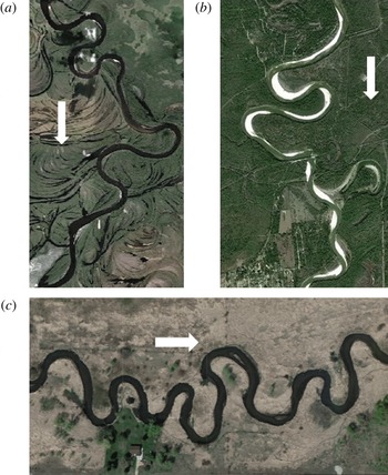
Most of the observations of Brice (Reference Brice1982) and Lagasse et al. (Reference Lagasse, Spitz, Zevenbergen and Zachmann2004) were based on channel width defined from vegetation line to vegetation line. Figure 1 shows three reaches: the Ob River, Russia, the Trinity River, Texas, USA, and the Vermillion River, Minnesota, USA. All three reaches display a pattern of width variation that correlates with centreline curvature. In terms of vegetation line, the first two reaches tend to be wider at bend apexes (maximum curvature) relative to crossings (vanishing curvature). In the third reach, however, this pattern is reversed: the channel tends to be narrower at apexes. Channel width can also be defined, however, in terms of water margin to water margin. In the case of the Trinity River, figure 1(b) shows that the channel defined by vegetation lines is wider at apexes, but that the channel defined by water margins is narrower at apexes. The former may reflect bankfull flow conditions, whereas the latter reflects below-bankfull stage. This stage dependence has been pointed out by Luchi et al. (Reference Luchi, Zolezzi and Tubino2011).
Meandering river reaches showing width variation: (a) Ob River, Russia; (b) Trinity River, Texas, USA; (c) Vermillion River, Minnesota, USA. Arrows indicate direction of flow. For scale, typical river widths are 150, 190 and 15 m for cases (a), (b) and (c), respectively. The images are from Google Earth.

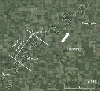
In order to analyse width-curvature relations, we used reaches of the Vermillion River near Empire, MN and the Trinity River downstream of Livingston Dam in Eastern Texas (figure 1). We also studied the reach of the Pembina River near Rossington in Alberta, Canada (figure 2). Table 1 gives the characteristics of each reach. The data sources are as follows: Vermillion River, Lauer & Parker (Reference Lauer and Parker2008); Trinity River, Smith (Reference Smith2012); Pembina River, Beck et al. (Reference Beck, Harrington and Andres1983). All three reaches are highly sinuous and actively migrating (Beck et al. Reference Beck, Harrington and Andres1983; Lauer & Parker Reference Lauer and Parker2008; Smith Reference Smith2012).
Study reach of the Pembina River Reach in Alberta, Canada. The arrow indicates direction of flow.

Characteristics of study reaches.

The channel banklines were digitized from aerial photographs using visible vegetation lines, and the channel centreline was obtained from digitized banklines in a way similar to Lauer & Parker (Reference Lauer and Parker2008). Local half-widths were obtained during the iterative procedure as the tangential distance from the centreline to the bank line at each node.
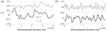
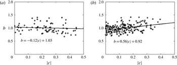
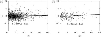
Figure 3 shows the downstream variation in curvature and width for the Vermillion and the Trinity River reaches. Figure 4 shows linear regressions of half-width against curvature for each reach. Here dimensionless curvature
 $c$
and half-width
 $b$
are
 $$\begin{eqnarray}c=\frac{\tilde{b}_{o}}{\tilde{R}_{c}};\quad b=\frac{\tilde{b}}{\tilde{b}_{o}}\end{eqnarray}$$
where
 $\tilde{b}$
and
 $\tilde{R}_{c}$
denote local half-width and centreline radius of curvature, respectively, and
 $\tilde{b}_{o}$
denotes the reach-averaged channel half-width. Again, tildes denote dimensioned parameters.
Downchannel variation of dimensionless centreline curvature and dimensionless channel half-width: (a) Vermillion River; (b) Trinity River.

Linear regressions of dimensionless channel half-width and dimensionless centreline curvature correlation: (a) Vermillion River; (b) Trinity River. The stars indicate the data.

The cases of the Vermillion and Trinity River reaches of figures 3 and 4 highlight the range of tendencies in width variation in meandering rivers. In the Vermillion River, points near the crossings (
 $c\sim 0$
) tend to be wider than points near the apexes (
 $c\sim 0.3$
), but the variation is weak (fractional width variation of
 $-$
0.04 as
 $c$
varies from 0 to 0.35). In the Trinity River, points near apexes tend to be wider than those near crossings, and the variation is notably stronger (fractional variation of 0.19 as
 $c$
varies from 0 to 0.35).
The pattern observed for the Trinity River is in general agreement with the trends reported in Brice (Reference Brice1982) and Lagasse et al. (Reference Lagasse, Spitz, Zevenbergen and Zachmann2004). Field data on more than 1500 meander bends reported by Lagasse et al. (Reference Lagasse, Spitz, Zevenbergen and Zachmann2004) indicate that maximum values of channel width tend to be close to bend apexes and minimum width values tend to be near inflections. Within a subset having significant width variations (type C of the Brice (Reference Brice1975) classification), width tended to be 14 % larger at apexes than at inflections.
The reach of the Pembina River in figure 2 is of particular interest, because the relevant parameters are used below in implementations of our model. Here we study the entire reach shown in figure 2, along with the Manola subreach which has shown rapid migration in recent geomorphic time (Beck et al.
Reference Beck, Harrington and Andres1983). Figure 5(a,b) show the correlations between
 $b$
and
 $c$
for the entire reach and the Manola subreach. Over the entire reach, the fractional variation in width is 0.03 as
 $c$
increases from 0 to 0.35; in the Manola subreach it is 0.09.
Linear regression of dimensionless channel half-width and dimensionless centreline curvature correlation for the Pembina River. (a) The entire Pembina reach near Rossington. (b) Manola subreach. The ‘
 $\times$
’ indicate the data and the lines are linear fits to the data.

The observations presented here for the Vermillion, Trinity and Pembina Rivers, combined with the earlier analyses of Lagasse et al. (Reference Lagasse, Spitz, Zevenbergen and Zachmann2004) suggest the following: meandering rivers may evolve so as to (a) have little systematic width variation, (b) show apexes that are slightly narrower than crossings or (c) show apexes that are slightly to significantly wider than crossings. Case (c) appears to be most common in rivers that show significant rates of migration.
The above picture is supported by results on the Lower Trinity River, TX, reported by Peyret (Reference Peyret2011) and Smith (Reference Smith2012). The Trinity River reach shown in figure 1 is part of the Lower Trinity River, TX and is sandwiched between two low migration reaches: an upstream incising reach influenced by the presence of the Livingston Dam and a downstream backwater reach that feeds into the Trinity Bay. Peyret (Reference Peyret2011) has shown that width is weakly and negatively correlated with centreline curvature in zones of low migration rate, whereas it is more strongly and positively correlated to curvature in zones where the river shows higher migration rates.
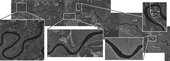
Plots of the type of figures 4 and 5 are intended to illustrate trends, rather than to illustrate predictive relations. They do not give a complete picture of width variation, because they do not specify the locations of minimum and maximum width relative to bend apexes. We address this with planform data from reaches of two rivers in Florida, USA: the Apalachicola and Suwannee Rivers. These rivers have dense bank vegetation, which makes quantification of width variation straightforward. The segment of the Suwannee River shown in figure 6 starts just north of Wannee in Gilchrist County, Florida, and ends at Fowler Bluff in Levee County, Florida. The segment of the Apalachicola River extends from New Hope, south of the Blountstown Gage, to the intersection between the Gulf County border to the north and the Liberty County border to the west.
View of the study reach of the Suwannee River. Flow is from left to right. The bend in the leftmost insert has a minimum width of 68 m and a maximum width of 104 m.

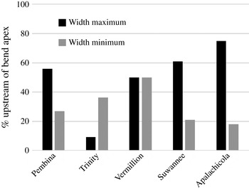
An analysis 33 bends of the Suwannee River indicates that the point of maximum width is located upstream of the bend apex, i.e. between the apex and the nearest crossing upstream, in 61 % of cases; in the other cases, maximum width was located between the apex and the next crossing downstream. A corresponding analysis of the Apalachicola River showed that the point of maximum width is reached upstream of the apex in 75 % of 44 bends. Evidently, these rivers have a strong bias for maximum width to occur between the apex and the nearest crossing upstream.
That this behaviour is not universal is illustrated in figure 7. The Pembina River is similar to the Apalachicola and Suwannee Rivers, with width maximums preferentially located upstream of bend apexes. In the case of the Vermillion, the position of width maximum is equally split between upstream and downstream, and in the case of the Trinity River, width maximum is located preferentially downstream of bend apex.
Percentage of bends in which the location of the width maximum and width minimum are upstream of the bend apex for five river reaches: the Pembina River, the Trinity River, the Vermillion River, the Suwannee River and the Apalachicola River.

Also shown in figure 7 is the percentage of bends for which the width minimum is located upstream of the bend apex. It is seen that in all cases but the Vermillion River, the point of width minimum tends to be located downstream of the bend apex. In the case of the Vermillion River, there is an equal likelihood for the width minimum to be located upstream or downstream of the apex.
Whether or not a migrating, meandering river shows correlation between the spatial variations of width and curvature, where maximum width is attained relative to bend apex, are determined by the internal dynamics of river itself. This dynamical picture cannot be understood without a model for width evolution itself. An attempt at developing such a model has been presented in Parker et al. (Reference Parker, Shimizu, Wilkerson, Eke, Abad, Lauer, Paola, Dietrich and Voller2011) and Eke (Reference Eke2013). The analysis below applies this model in order to investigate the relation between width and curvature.
3. Width of an equivalent straight channel: bankfull geometry
Before exploring how meander planform and width variation coevolve, it is necessary to specify a closure model for width that is applicable to an equivalent straight channel. More generally, we pursue a model for bankfull channel geometry. We consider a channel with characteristic bed material size
 $\tilde{D}_{s}$
, and for which the dominant model of bed material transport is bedload. Let
 $\tilde{Q}_{o}$
and
 $\tilde{Q}_{so}$
be the bankfull water discharge and volume bedload transport rate at bankfull flow, respectively, and
 $S_{o}$
denote the reach-averaged bed slope of a meandering reach. The bankfull half-width and bankfull depth of an equivalent straight reach at this slope are
 $\tilde{b}_{o}$
and
 $\tilde{H}_{o}$
. Bankfull flow velocity
 ${\tilde{U}}_{o}$
is given according to the relation
 $$\begin{eqnarray}\tilde{Q}_{o}=2\tilde{b}_{o}\tilde{H}_{o}{\tilde{U}}_{o}.\end{eqnarray}$$
In addition,
 $\tilde{Q}_{so}$
is related to the volume bedload transport rate per unit width
 $\tilde{q}_{so}$
according to the relation
 $$\begin{eqnarray}\tilde{Q}_{so}=2\tilde{b}_{o}\tilde{q}_{so}.\end{eqnarray}$$
Bankfull streamwise bed shear stress
 $\tilde{{\it\tau}}_{sbf}$
is related to bankfull flow velocity
 ${\tilde{U}}_{o}$
as
 $$\begin{eqnarray}\tilde{{\it\tau}}_{sbf}={\it\rho}C_{f}{\tilde{U}}_{o}^{2}\end{eqnarray}$$
where
 $C_{f}$
is a dimensionless bed friction coefficient and
 ${\it\rho}$
is (dimensioned) water density. The dimensionless parameter corresponding to channel-forming (i.e. bankfull) Shields number
 ${\it\tau}_{form}^{\ast }$
can be defined as
 $$\begin{eqnarray}{\it\tau}_{form}^{\ast }=\frac{\tilde{{\it\tau}}_{sbf}}{{\it\rho}Rg\tilde{D}_{s}}\end{eqnarray}$$
where
 $R$
is the (dimensionless) submerged specific gravity of the sediment (1.65 for quartz) and
 $g$
is (dimensioned) gravitational acceleration.
As outlined in Eke et al. (Reference Eke, Parker and Shimizu2014), the constraints of (a) normal flow momentum balance, (b) a bedload transport relation, (c) a specified channel-formative (bankfull) Shields number
 ${\it\tau}_{form}^{\ast }$
and (d) specified grain size
 $\tilde{D}_{s}$
result in four constraints on the five parameters
 $\tilde{Q}_{o}$
,
 $\tilde{Q}_{so}$
,
 $\tilde{b}_{o}$
,
 $\tilde{H}_{o}$
and
 $S_{o}$
. Normal flow momentum balance takes the form
 $$\begin{eqnarray}\tilde{{\it\tau}}_{sbf}={\it\rho}g\tilde{H}_{o}S_{o}\end{eqnarray}$$
Here we use the Parker (Reference Parker1979) approximation of the Einstein (Reference Einstein1950) relation for bedload transport applied to bankfull flow:
 $$\begin{eqnarray}\tilde{q}_{so}=11.2\sqrt{Rg\tilde{D}_{s}}\,\tilde{D}_{s}\left({\it\tau}_{form}^{\ast }\right)^{1.5}\left[1-\frac{{\it\tau}_{c}^{\ast }}{{\it\tau}_{form}^{\ast }}\right]^{4.5}\end{eqnarray}$$
where
 ${\it\tau}_{c}^{\ast }$
takes the value 0.03. Reduction of the above relations yields the three constraints:
 $$\begin{eqnarray}\displaystyle & S_{o}=\frac{R}{11.2C_{f}^{1/2}\left[\displaystyle 1-\frac{{\it\tau}_{c}^{\ast }}{{\it\tau}_{form}^{\ast }}\right]^{4.5}}\left(\displaystyle \frac{\tilde{Q}_{so}}{\tilde{Q}_{0}}\right) & \displaystyle\end{eqnarray}$$
 $$\begin{eqnarray}\displaystyle & 2\tilde{b}_{0}=\displaystyle \frac{\tilde{Q}_{s0}}{\displaystyle 11.2\left({\it\tau}_{form}^{\ast }\right)^{1.5}\left[1-\displaystyle \frac{{\it\tau}_{c}^{\ast }}{{\it\tau}_{form}^{\ast }}\right]^{4.5}\sqrt{Rg\tilde{D}_{s}}\tilde{D}_{s}} & \displaystyle\end{eqnarray}$$
 $$\begin{eqnarray}\displaystyle & \tilde{H}_{o}=11.2{\it\tau}_{form}^{\ast }\left[1-\displaystyle \frac{{\it\tau}_{c}^{\ast }}{{\it\tau}_{form}^{\ast }}\right]^{4.5}C_{f}^{1/2}\tilde{D}_{s}\left(\displaystyle \frac{\tilde{Q}_{o}}{\tilde{Q}_{so}}\right). & \displaystyle\end{eqnarray}$$
 $\tilde{D}_{s}$
and channel-forming Shields number are specified, the slope, width and depth of the channel can be computed from (3.7)–(3.9).
In the context of the present model, the specified parameters are bankfull discharge
 $\tilde{Q}_{o}$
, grain size
 $\tilde{D}_{s}$
and reach-averaged bed slope
 $S_{o}$
corresponding to a sinuous channel at a given time. In earlier implementations of the above formulation (as summarized by Li et al.
Reference Li, Czapiga, Eke, Viparelli and Parker2014),
 ${\it\tau}_{form}^{\ast }$
was taken to be a specified parameter, taking one value for sand-bed rivers and another value for gravel-bed rivers. As shown therein, this assumption imposes an unrealistic constraint on meandering rivers.
MacDonald, Parker & Leuthe (Reference MacDonald, Parker and Leuthe1991) provide a compendium of data for 16 reaches of migrating, meandering rivers in Minnesota, USA. The sinuosity of these reaches varies from 1.21 to 2.61. Now consider a river reach that is initially nearly straight with bed slope
 $S_{oi}$
, but that evolves toward a tortuous state over time. According to (3.7) and (3.8) and the constraints of constant
 $C_{f}$
and
 ${\it\tau}_{form}^{\ast }$
, as
 $S_{o}$
drops from the straight-channel value
 $S_{oi}$
to one corresponding to a sinuosity of 2.5, i.e. 0.4
 $S_{oi}$
, width should correspondingly drop to 40 % of its value at the nearly straight state. No such sharp drop in width with increasing sinuosity is observed in general, and in particular in the data set of MacDonald et al. (Reference MacDonald, Parker and Leuthe1991).
The resolution to this conundrum is contained in Li et al. (Reference Li, Czapiga, Eke, Viparelli and Parker2014). They use empirical data to demonstrate the following relation for channel-forming (bankfull) Shields number, across the range from silt-bed to cobble-bed rivers:
 $$\begin{eqnarray}{\it\tau}_{form}^{\ast }=1220\,(D^{\ast })^{-1}\,S^{0.53}\end{eqnarray}$$
where
 $D^{\ast }$
is a dimensionless grain size defined as
 $$\begin{eqnarray}D^{\ast }=\frac{\left(Rg\right)^{1/3}}{{\it\nu}^{2/3}}D_{s}\end{eqnarray}$$
and
 ${\it\nu}$
denotes (dimensioned) kinematic viscosity of water. According to (3.10), as the sinuosity of a reach increases, and thus as the reach-averaged bed slope
 $S_{o}$
drops,
 ${\it\tau}_{form}^{\ast }$
drops accordingly. This effect, when embedded in (3.7) and (3.8), results in modest, rather than extreme channel narrowing as sinuosity increases, as illustrated subsequently in this paper.
The formulation for width-planform coevolution pursued herein is based on deviation from the channel-forming Shields number. The flow under consideration is bankfull, but bed shear stress now varies spatially because of a meandering planform. The flow field, including bed shear stress, is computed in a submodel for in-channel morphodynamics. Adjacent to a bank, the streamwise bed shear stress may be above or below the value corresponding to channel-forming flow. In the former case, the bank is eroded according to a submodel capturing sediment removal mitigated by armouring due to slump blocks. In the latter case, the bank accretes according to a submodel capturing vegetal encroachment mitigated by increasing strength of near-bank flow.
4. Model formulation for a meandering channel
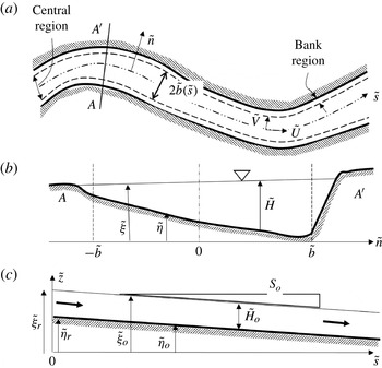
Our model formulation follows the framework of Parker et al. (Reference Parker, Shimizu, Wilkerson, Eke, Abad, Lauer, Paola, Dietrich and Voller2011). We define three distinct regions as shown in figure 8: a central channel of width
 $2\tilde{b}(\tilde{s})$
and two bank regions, where
 $\tilde{b}(\tilde{s})$
is the local channel half-width and
 $\tilde{s}$
denotes a streamwise centreline coordinate (the tildes denote dimensioned parameters). Within the central region, a steady-state nonlinear flow and bed morphodynamics model is applied to determine in-channel characteristics. The bank region characteristics (e.g. bank height and bank slope) are specified input parameters and bank migration is modelled via shock conditions that determine the migration rate of the bank toe.
Definition sketch of channel (a) planform, (b) cross-section and (c) reference straight channel. Modified from Beck et al. (Reference Beck, Harrington and Andres1983).

The model uses an assumption that is akin to the standard quasi-steady assumption of river bed morphodynamics (de Vries Reference de Vries1965). It is assumed that the planform processes associated with bankline migration are sufficiently slow compared to both hydraulic and in-channel bed morphodynamic processes that at the time scale of planform evolution, the flow and bed can be approximated as steady state. This assumption, which is commonly used in other models of meander planform evolution as well (e.g. Frascati & Lanzoni Reference Frascati and Lanzoni2009) significantly reduces computation time, and allows for the model to be run at larger spatial and temporal scales. The drawback of this assumption is that the model cannot incorporate the formation of free bars migrating through a train of bends. Thus, we do not describe in detail the mechanism of bank collapse and the subsequent process of sediment removal followed by sediment redistribution downstream. Rather, we assume that this redistribution occurs at bed morphodynamic time scale, but adjust the mean bed accordingly at the longer scale of bankline migration.
4.1. In-channel morphodynamic submodel for channel of varying width
As shown in figure 8, the model uses an intrinsic curvilinear coordinate system to describe the channel planform. In this coordinate system, the streamwise coordinate
 $\tilde{s}$
corresponds to the channel centreline and the local transverse coordinate
 ${\tilde{n}}$
is defined to be orthogonal to the channel centreline, and is always taken as increasing toward the left bank of the river looking downstream. This transverse coordinate varies from
 $-\tilde{b}(\tilde{s},\tilde{t})$
to
 $\tilde{b}(\tilde{s},\tilde{t})$
as shown in figure 8(b).
The equations governing channel hydrodynamics/morphodynamics are presented below. Unless otherwise specified, dimensioned parameters introduced below are denoted so with a tilde superscript; the corresponding parameters without a tilde are dimensionless. Relevant scales for the non-dimensionalization are the previously introduced dimensioned depth-averaged streamwise flow velocity
 ${\tilde{U}}_{o}$
, flow depth
 $\tilde{H}_{o}$
and mean channel half-width
 $\tilde{b}_{o}$
, all in a reference straight channel as defined in figure 8(c). These reference quantities, as well as the reference sediment transport rate
 $\tilde{Q}_{so}$
are time-dependent, so as to account for changes in reach-average characteristics as meanders migrate, as indicated in (4.38) below. The Froude number
 $F_{o}$
and ratio of half-width to depth
 ${\it\gamma}_{o}$
of the base flow are given as
 $$\begin{eqnarray}F_{o}=\frac{{\tilde{U}}_{o}}{\sqrt{g\tilde{H}_{o}}};\quad {\it\gamma}_{o}=\frac{\tilde{b}_{o}}{\tilde{H}_{o}}.\end{eqnarray}$$
We introduce the following dimensionless parameters:
 $s$
and
 $n$
denote dimensionless streamwise and transverse coordinates, respectively,
 $U$
and
 $V$
denote dimensionless, depth-averaged streamwise and transverse flow velocities, respectively,
 $H$
denotes dimensionless depth,
 $c$
denotes dimensionless channel centreline curvature and
 ${\it\xi}$
denotes dimensionless water surface elevation, defined as
 $$\begin{eqnarray}s=\frac{\tilde{s}}{\tilde{b}_{o}};\quad n=\frac{{\tilde{n}}}{\tilde{b}};\quad b=\frac{\tilde{b}}{\tilde{b}_{o}};\quad (U,V)=\frac{\left({\tilde{U}},\tilde{V}\right)}{{\tilde{U}}_{o}};\quad \left(H,{\it\xi}\right)=\frac{\left(\tilde{H},\tilde{{\it\xi}}\right)}{\tilde{H}_{o}};\quad c=\frac{\tilde{b}_{o}}{\tilde{R}_{c}}\end{eqnarray}$$
where
 $\tilde{R}_{c}$
is the local centreline radius of curvature. Note here that the transverse coordinate
 $n$
defined above has been rescaled with the local channel width
 $\tilde{b}(s)$
for geometric simplicity so that the dimensionless coordinate
 $n$
always ranges from
 $-$
1 to 1. The parameters (
 ${\it\tau}_{s}$
,
 ${\it\tau}_{n}$
) denote dimensionless streamwise and transverse bed shear stresses, respectively, and (
 $q_{s},q_{n}$
) denote dimensionless streamwise and transverse volume sediment transport rates per unit width, respectively: they are defined in terms of their corresponding dimensioned variables as
 $$\begin{eqnarray}\left({\it\tau}_{s},{\it\tau}_{n}\right)=\frac{\left(\tilde{{\it\tau}}_{s},\tilde{{\it\tau}}_{n}\right)}{{\it\rho}{\tilde{U}}_{o}^{2}};\quad \left(q_{s},q_{n}\right)=\frac{\left(\tilde{q}_{s},\tilde{q}_{n}\right)}{\sqrt{Rg\tilde{D}_{s}}\tilde{D}_{s}}.\end{eqnarray}$$
The dimensionless steady-state depth-averaged equations of motion for a general fluid flow with variable width can thus be written in intrinsic curvilinear coordinates as follows:
 $$\begin{eqnarray}\displaystyle & \displaystyle \frac{\partial HV}{\partial n}+NbcVH+bL_{sn}\left(UH\right)=0 & \displaystyle\end{eqnarray}$$
 $$\begin{eqnarray}\displaystyle & \displaystyle V\frac{\partial U}{\partial n}+UbL_{sn}\left(U\right)+bNcU\left(V+2{\it\varphi}\right)+\frac{1}{H}\frac{\partial HU{\it\varphi}}{\partial n}=-\frac{1}{F_{o}^{2}}bL_{sn}\left({\it\xi}\right)-b\frac{{\it\gamma}_{o}{\it\tau}_{s}}{H} & \displaystyle\end{eqnarray}$$
 $$\begin{eqnarray}\displaystyle & & \displaystyle \displaystyle V\frac{\partial V}{\partial n}+UbL_{sn}\left(V\right)+Nbc\left(2V{\it\varphi}+{\it\psi}-U^{2}\right)+2\frac{1}{H}\frac{\partial HV{\it\varphi}}{\partial n}+\frac{1}{H}\frac{\partial H{\it\psi}}{\partial n}+\frac{1}{H}bL_{sn}\left(UH{\it\varphi}\right)\nonumber\\ \displaystyle & & \displaystyle \displaystyle \quad =-F_{o}^{-2}\frac{\partial {\it\xi}}{\partial n}-b\frac{{\it\gamma}_{o}{\it\tau}_{n}}{H}\end{eqnarray}$$
 $L_{sn}$
is a differential operator given as
 $$\begin{eqnarray}L_{sn}=N\left(\frac{\partial }{\partial s}-\frac{n}{b}\frac{\text{d}b}{\text{d}s}\frac{\partial }{\partial n}\right).\end{eqnarray}$$
Here,
 $N$
is the longitudinal metric coefficient of the coordinate system, i.e.
 $$\begin{eqnarray}N=\left(1+nbc\right)^{-1}\end{eqnarray}$$
and the parameters
 ${\it\varphi}$
and
 ${\it\psi}$
in (4.4) and (4.6) are secondary flow redistribution terms defined in Eke et al. (Reference Eke, Parker and Shimizu2014).
The Exner equation of bed sediment conservation is given as
 $$\begin{eqnarray}bL_{sn}\left(q_{s}\right)+\frac{\partial q_{n}}{\partial n}+q_{n}Nbc=0.\end{eqnarray}$$
Closures for the components of bed shear stress and bedload transport are as given in Eke et al. (Reference Eke, Parker and Shimizu2014), i.e.
 $$\begin{eqnarray}\displaystyle \left({\it\tau}_{s},{\it\tau}_{n}\right)=C_{f}\sqrt{U^{2}+V^{2}}\left(U,V+\frac{{\it\nu}_{s}(0)}{T(0)}\right) & & \displaystyle\end{eqnarray}$$
 $$\begin{eqnarray}\displaystyle \left(q_{s},q_{n}\right)={\it\Phi}\left(\cos {\it\vartheta},\sin {\it\vartheta}\right)\cong {\it\Phi}\left(1,\frac{{\it\tau}_{n}^{\ast }}{{\it\tau}_{s}^{\ast }}-\frac{r}{{\it\gamma}_{o}\sqrt{{\it\tau}_{o}^{\ast }}}\frac{\partial {\it\eta}}{\partial n}\right) & & \displaystyle\end{eqnarray}$$
 ${\it\nu}_{s}$
denotes dimensionless secondary flow (made dimensionless by the streamwise velocity
 ${\tilde{U}}_{o}$
,
 $C_{f}$
is the bed friction coefficient (here assumed to be a constant),
 $T$
is a primary flow structure function (Johannesson & Parker Reference Johannesson, Parker, Ikeda and Parker1989),
 ${\it\vartheta}$
indicates the angle of direction of sediment transport relative to the channel centreline,
 $r$
is a coefficient ranging from 0.3 to 1 (see also Johannesson & Parker Reference Johannesson, Parker, Ikeda and Parker1989). Here
 ${\it\tau}_{s}^{\ast }$
and
 ${\it\tau}_{n}^{\ast }$
are the dimensionless Shields stresses given as
 $$\begin{eqnarray}\left({\it\tau}_{s}^{\ast },{\it\tau}_{n}^{\ast }\right)=\frac{{\tilde{U}}_{o}^{2}}{gR\tilde{D}_{s}}\left({\it\tau}_{s},{\it\tau}_{n}\right)\end{eqnarray}$$
and
 ${\it\Phi}$
is the bedload transport intensity, here estimated using the relation of Parker (Reference Parker1979):
 $$\begin{eqnarray}{\it\Phi}=11.2\left({\it\tau}_{s}^{\ast }\right)^{1.5}\left[1-\frac{0.03}{{\it\tau}_{s}^{\ast }}\right]^{4.5}.\end{eqnarray}$$
The approximation for secondary flow adopted here is derived from the case of steady, uniform bend flow; and has been generalized to a channel of arbitrary curvature:
 $$\begin{eqnarray}{\it\nu}_{s}=\frac{UH}{{\it\chi}_{1}{\it\gamma}_{o}C_{f}}cG\end{eqnarray}$$
where
 $G$
is the normalized secondary flow structure function defined in Johannesson & Parker (Reference Johannesson, Parker, Ikeda and Parker1989) and
 ${\it\chi}_{1}=C_{f}^{-1/2}/13$
(see also Seminara & Solari Reference Seminara and Solari1998; Bolla Pittaluga, Nobile & Seminara Reference Bolla Pittaluga, Nobile and Seminara2009). More advanced nonlinear, approaches to secondary flow, e.g. Ottevanger, Blanckaert & Uijttewaal (Reference Ottevanger, Blanckaert and Uijttewaal2012) are available, but a linear approach is more suitable for a first model of meandering channels with self-formed width.
The lateral boundary conditions associated with (4.4)–(4.6) and (4.9) are no-penetration conditions for the flow and sediment transport, respectively. Thus,
 $\boldsymbol{U}\boldsymbol{\cdot }\hat{\boldsymbol{n}}_{b}=\boldsymbol{q}\boldsymbol{\cdot }\hat{\boldsymbol{n}}_{b}=0$
, where
 $\boldsymbol{U}$
and
 $\boldsymbol{q}$
are the velocity and bedload transport vectors respectively and
 $\hat{\boldsymbol{n}}_{b}$
is the unit vector normal to the banks. This translates to
 $$\begin{eqnarray}\displaystyle -\frac{U}{\left(1\pm bC\right)}\frac{\text{d}b}{\text{d}s}\pm V=0\quad \text{at}\ n=\pm 1 & & \displaystyle\end{eqnarray}$$
 $$\begin{eqnarray}\displaystyle -\frac{q_{s}}{\left(1\pm bC\right)}\frac{\text{d}b}{\text{d}s}\pm q_{n}=0\quad \text{at}\ n=\pm 1. & & \displaystyle\end{eqnarray}$$
Finally, the imposed integral conditions for the conservation of water and sediment discharge within the channel are as follows:
 $$\begin{eqnarray}\displaystyle b\int _{-1}^{1}UH\,\text{d}n=2 & & \displaystyle\end{eqnarray}$$
 $$\begin{eqnarray}\displaystyle b\int _{-1}^{1}q_{s}\,\text{d}n=2q_{so} & & \displaystyle\end{eqnarray}$$
 $q_{so}$
is the streamwise bedload transport rate for the reference straight channel. The integral conditions (4.17) and (4.18) specify that the water discharge and sediment discharge in the channel respectively remain the same as for a reference straight channel, regardless of sinuosity. As a result, the average channel slope
 $S$
becomes a free variable represented by the deviation
 $s_{do}$
from the reference channel slope
 $S_{o}$
, such that
 $$\begin{eqnarray}S=S_{o}(1+s_{do}).\end{eqnarray}$$
Nonlinear effects assure that in the case of a bend with the same average width, the same sediment transport rate is realized at a lower average bed slope than the case of a straight channel (e.g. Luchi et al.
Reference Luchi, Bolla Pittaluga and Seminara2012). In keeping with (4.19), constant deviatoric velocity and depth parameters,
 $u_{do}$
and
 $h_{do}$
respectively, arise which in the presence of sinuosity allow total reach-averaged velocity and flow depth to differ from the values corresponding to the reference straight channel. Thus,
 $$\begin{eqnarray}\tilde{H}_{mean}=\tilde{H}_{o}(1+h_{do});\quad {\tilde{U}}_{mean}={\tilde{U}}_{o}(1+u_{do}).\end{eqnarray}$$
At the linear level, however, the reach-averaged values of velocity, bed slope and depth are found to be identical to the reference values (e.g. Imran et al. Reference Imran, Parker and Pirmez1999).
The method to arrive at an iterative solution of the nonlinear system of equations is as outlined in Imran et al. (Reference Imran, Parker and Pirmez1999) and Camporeale et al. (Reference Camporeale, Perona, Porporato and Ridolfi2007). Herein we go a step further to include the added complexity of width variation to the solution outlined in Camporeale et al. (Reference Camporeale, Perona, Porporato and Ridolfi2007). Our method involves expressing each morphodynamic variable as the sum of that for a reference straight channel and a deviation due to the combined effect of channel curvature and width variation. Thus, local variables are expressed as follows:
 $$\begin{eqnarray}\displaystyle \left(U,V,H,{\it\eta},{\it\xi},c,b\right) & = & \displaystyle \left[1,0,1,{\it\eta}_{r}-S_{o}s,{\it\xi}_{r}+1-S_{o}s,0,1\right]+\left(u_{do}+u_{d},v_{d},h_{do}+h_{d},\right.\nonumber\\ \displaystyle & & \displaystyle \left.-S_{o}s_{do}s+{\it\eta}_{d},h_{do}-S_{o}s_{do}s+{\it\xi}_{d},c,b_{d}\right)\end{eqnarray}$$
where
 $h_{d}={\it\xi}_{d}-{\it\eta}_{d}$
, the subscript ‘
 $d$
’ denotes the deviation and
 ${\it\xi}_{r},{\it\eta}_{r}$
are the reference water and bed elevation as shown in figure 6(c). In the above equations,
 $u_{do},\ s_{do}$
and
 $h_{do}$
denote the constant deviatoric streamwise velocity, slope and water depth, respectively, which correspond to reach-averaged conditions and are independent of
 $s$
and
 $n$
.
Meanwhile,
 $q_{s}$
is taken to be a nonlinear function of
 $U$
such that
 $q_{s}=1$
where
 $U=1$
. As defined in (4.11) and (4.13),
 $q_{s}$
is evaluated from the relation of Parker (Reference Parker1979) and can be expressed in the form of a Taylor expansion, i.e.
 $$\begin{eqnarray}q_{s}=11.2\left({\it\tau}_{s}^{\ast }\right)^{1.5}\left[1-\frac{0.03}{{\it\tau}_{s}^{\ast }}\right]^{4.5}=q_{so}\left(1+M\left(U-1\right)+R_{q}\left(U\right)\right)\end{eqnarray}$$
where
 $M=2({\it\tau}_{o}^{\ast }/q_{so})(\partial q_{s}/\partial {\it\tau}^{\ast })|_{{\it\tau}={\it\tau}_{o}}$
. The above equation illustrates the approach to the nonlinear problem presented here;
 $R_{q}$
represents the difference between the full sediment transport relation and its linear form, or thus the nonlinear residual.
The deviations
 $u_{d},{\it\eta}_{d}$
and
 ${\it\xi}_{d}$
can be further decomposed as follows:
 $$\begin{eqnarray}\displaystyle \left.\begin{array}{@{}l@{}}u_{d}=u_{dd}(s,n)+u_{dc}(s)\\ {\it\eta}_{d}={\it\eta}_{dd}(s,n)+{\it\eta}_{dc}(s)\\ {\it\xi}_{d}={\it\xi}_{dd}(s,n)+{\it\xi}_{dc}(s).\end{array}\right\} & & \displaystyle\end{eqnarray}$$
Here
 $u_{dc}$
,
 ${\it\xi}_{dc}$
and
 ${\it\eta}_{dc}$
denote the cross-sectionally averaged deviations of streamwise velocity
 $u_{d}$
, water surface elevation
 ${\it\xi}_{d}$
, and bed elevation
 ${\it\eta}_{d}$
, respectively. As such, they are functions of streamwise coordinate
 $s$
only. In addition, the parameters
 $u_{dd}$
,
 ${\it\xi}_{dd}$
and
 ${\it\eta}_{dd}$
represent functional forms for the corresponding differences
 $u_{d}-u_{dc}$
,
 ${\it\xi}_{d}-{\it\xi}_{dc}$
and
 ${\it\eta}_{d}-{\it\eta}_{dc}$
; they depend on
 $s$
and
 $n$
, and characterize the transverse variations of streamwise velocity, water surface elevation and bed elevation. By definition, the parameters
 $u_{dd},{\it\xi}_{dd}$
and
 ${\it\eta}_{dd}$
must satisfy the conditions
 $$\begin{eqnarray}\int _{-1}^{1}u_{dd}\,\text{d}n=0,\quad \int _{-1}^{1}{\it\xi}_{dd}\,\text{d}n=0,\quad \int _{-1}^{1}{\it\eta}_{dd}\,\text{d}n=0.\end{eqnarray}$$
In addition,
 $u_{dc},{\it\xi}_{dc}$
and
 ${\it\eta}_{dc}$
are assumed to be periodic with wavelength
 ${\it\lambda}$
, and must satisfy the following conditions:
 $$\begin{eqnarray}\int _{0}^{{\it\lambda}}u_{dc}\,\text{d}s=0,\quad \int _{0}^{{\it\lambda}}{\it\eta}_{dc}\,\text{d}s=0,\quad \int _{0}^{{\it\lambda}}{\it\xi}_{dc}\,\text{d}s=0.\end{eqnarray}$$
At this point, it is seen that 10 unknowns,
 $u_{do},S_{do},h_{do},u_{dc},{\it\xi}_{dc},{\it\eta}_{dc},u_{dd},{\it\xi}_{dd},{\it\eta}_{dd}$
and
 $v_{d}$
appear in the above equations. According to these variables, three types of problems are defined: the ‘O’ problem with unknowns
 $u_{do}$
,
 $S_{do}$
and
 $h_{do}$
independent of
 $s$
and
 $n$
; the ‘C’ problem with unknowns
 $u_{dc},{\it\xi}_{dc}$
and
 ${\it\eta}_{dc}$
which are function of
 $s$
only; and the ‘D’ problem with unknowns
 $u_{dd},{\it\xi}_{dd},{\it\eta}_{dd}$
and
 $v_{d}$
which are functions of
 $s$
and
 $n$
. The methods of solution of each of these problems, which start from a linear formulation and use successive approximation so as to incorporate nonlinear residuals, are given in appendix A (‘D’ problem) and appendix B (‘O’ and ‘C’ problems).
4.2. Bank submodels
As stated previously, in order to generate width oscillations by channel migration, the standard channel centreline migration model proposed by Hasegawa (Reference Hasegawa1977) and Ikeda et al. (Reference Ikeda, Parker and Sawai1981) must be abandoned in favour of a model that allows each bank to migrate independently. The bank migration model formation proposed by Parker et al. (Reference Parker, Shimizu, Wilkerson, Eke, Abad, Lauer, Paola, Dietrich and Voller2011) and modified by Eke et al. (Reference Eke, Parker and Shimizu2014) quantifies this migration rate through a shock condition, which can be applied to either an eroding or depositing bank. For the sake of brevity, only a summary is given here; details can be found in Eke et al. (Reference Eke, Parker and Shimizu2014).
For any bank
 $j$
, which could be the left bank (LB) or right bank (RB), the lateral migration rate
 $\dot{{\tilde{n}}}_{j}$
is computed as
 $$\begin{eqnarray}\dot{{\tilde{n}}}_{j}=\tilde{{\it\zeta}}_{E}+\frac{1}{S_{s,j}}\frac{\partial \tilde{{\it\eta}}_{j}}{\partial \tilde{t}}\end{eqnarray}$$
for an eroding bank and
 $$\begin{eqnarray}\dot{{\tilde{n}}}_{j}=\tilde{{\it\zeta}}_{D}+\frac{1}{S_{s,j}}\frac{\partial \tilde{{\it\eta}}_{j}}{\partial \tilde{t}}\end{eqnarray}$$
for a depositing bank.
The terms
 $\tilde{{\it\zeta}}_{E}$
and
 $\tilde{{\it\zeta}}_{D}$
represent erosion and lateral accretion rates due to sediment transport away from and toward the banks, respectively. The second term on the right-hand side of (4.26) and (4.27) represent lateral migration due to bed elevation changes near the banks, where
 $\tilde{{\it\eta}}$
is the channel bed elevation and
 $\tilde{{\it\eta}}_{j}$
is the bed elevation at bank
 $j$
corresponding to the elevation at
 ${\tilde{n}}=\tilde{b}(\tilde{t})$
and
 ${\tilde{n}}=-\tilde{b}(\tilde{t})$
for the left and right bank, respectively, where
 ${\tilde{n}}$
is the transverse coordinate, defined so as to increase toward the left bank looking downstream, and
 $\tilde{b}$
is the half channel width. For simplicity, each bank
 $j$
here has been assumed to have a constant side slope
 $S_{s,j}$
.
Eke et al. (Reference Eke, Parker and Shimizu2014) details the process of deriving closures to quantify the erosion and deposition rates
 $\tilde{{\it\zeta}}_{E}$
and
 $\tilde{{\it\zeta}}_{D}$
in (4.26) and (4.27) above. These simple closures are expressed in terms of parameters of a fairly intuitive nature namely, an armouring coefficient
 $K_{armour}$
associated with slump block armouring of an eroding bank, a flood intermittency factor
 $I_{f}$
, a default rate of transverse migration
 ${\it\zeta}_{veg}$
in the absence of a near-bank shear stress that acts to suppress vegetation, and the erosional bank migration rate for a purely non-cohesive bank in the absence of slump block armouring
 ${\it\zeta}_{non,E}$
. Specifically, the closure relation specifying the erosion rate
 $\tilde{{\it\zeta}}_{E}$
is given as
 $$\begin{eqnarray}\tilde{{\it\zeta}}_{E}=K_{armour}I_{f}\tilde{{\it\zeta}}_{non,E}.\end{eqnarray}$$
That is to say, the erosion rate of a migrating channel corresponds to the erosion rate of the non-cohesive part of the bank for a channel with no bank armouring (for which
 $K_{armour}=1$
) during the fraction of time
 $I_{f}$
the river is in flood. This erosion rate reduces linearly with increased armouring (i.e. for
 $K_{armour}<1$
). Armouring in this model is considered to be through the presence of slump blocks of an upper cohesive, root-dense material, which form by e.g. undermining as a lower, non-cohesive part of the bank erodes. In the derivation of a functional form for this armouring coefficient, we have assumed that it is primarily a function of the erosion rate
 $\tilde{{\it\zeta}}_{E}$
(as more erosion produces more slump blocks), and slump block and cohesive layer properties. These properties include the height of the cohesive layer, the characteristic size of the slump blocks and the residence time of the blocks, which is assumed to be a function of the near-bank stresses. Thus,
 $$\begin{eqnarray}K_{armour}=K_{armour}\left(\tilde{{\it\zeta}}_{E},{\it\tau}_{E}^{\ast },\tilde{{\it\zeta}}_{Eref},{\it\tau}_{form}^{\ast }\right)\end{eqnarray}$$
where
 ${\it\tau}_{E}^{\ast }$
is the flow Shields number near the eroding bank,
 $\tilde{{\it\zeta}}_{Eref}$
is a reference erosion rate based purely on slump block characteristics and
 ${\it\tau}_{form}^{\ast }$
is a formative/threshold Shields number. The precise form of (4.29) is given by Eke et al. (Reference Eke, Parker and Shimizu2014). Substituting into (4.28), and rearranging, we get a simplified closure relation for
 $\tilde{{\it\zeta}}_{E}$
, namely
 $$\begin{eqnarray}\tilde{{\it\zeta}}_{E}=\frac{1}{\left(\displaystyle 1+\left(\frac{{\it\tau}_{E}^{\ast }}{{\it\tau}_{form}^{\ast }}-1\right)^{-1}I_{f,ref}\frac{|\tilde{{\it\zeta}}_{non,E}|}{\tilde{{\it\zeta}}_{Eref}}\right)}I_{f}\tilde{{\it\zeta}}_{non,E}.\end{eqnarray}$$
In (4.30), the parameter
 $I_{f,ref}$
is a reference intermittency corresponding to the reference erosion rate
 $\tilde{{\it\zeta}}_{Eref}$
. The relation in (4.30) is appreciated better if we assume the second term in the denominator is
 $\gg 1$
, in which case the form for the erosion rate simplifies to
 $$\begin{eqnarray}\tilde{{\it\zeta}}_{E}=\tilde{{\it\zeta}}_{Eref}\frac{I_{f}}{I_{f,ref}}\left(\frac{{\it\tau}_{E}^{\ast }}{{\it\tau}_{form}^{\ast }}-1\right).\end{eqnarray}$$
The formative Shields number here is the threshold value above which bank erosion occurs. As seen above, it also corresponds to the formative Shields number for a straight channel. The relation in (4.31) is very similar to the form of erosion rules that have been generally applied in previous work, with the difference being that terms have specifically defined closures based on measurable field parameters.
For a depositing/accreting bank, the model specifies a default rate of transverse migration
 $\tilde{{\it\zeta}}_{veg}$
of the inner accretional bank toward the channel centre associated with flows that are insufficient to suppress vegetation growth, i.e. during the fraction of time
 $1-I_{f}$
. The model then assumes a linear suppression of this encroachment rate as the near-bank bed shear stress increases, so that
 $$\begin{eqnarray}\tilde{{\it\zeta}}_{D}=\tilde{{\it\zeta}}_{veg}\left(1-I_{f}\right)\left(1-\frac{{\it\tau}_{D}^{\ast }}{{\it\tau}_{form}^{\ast }}\right)\end{eqnarray}$$
where
 $\tilde{{\it\zeta}}_{D}$
is a rate of transverse migration of the inner accretionary bank toward the channel centre and
 ${\it\tau}_{D}^{\ast }$
is the Shields number based on the streamwise shear stress acting on the bed immediately adjacent to the depositing bank. Again here we have assumed the formative Shields number to be a threshold above which lateral accretion is no longer possible.
The closures as presented in (4.30) and (4.32) allow a smooth transition from one process to the other, i.e. erosion occurs when
 ${\it\tau}_{j}^{\ast }\equiv {\it\tau}_{E}^{\ast }>{\it\tau}_{form}^{\ast }$
and accretion occurs where
 ${\it\tau}_{j}^{\ast }\equiv {\it\tau}_{D}^{\ast }<{\it\tau}_{form}^{\ast }$
where
 ${\it\tau}_{j}^{\ast }$
is the Shields number based on the streamwise bed shear stress immediately adjacent to a bank
 $j$
. Model bank input parameters thus include a specification of a relation for the formative Shields number
 ${\it\tau}_{form}^{\ast }$
, an estimation of the lumped reference migration rate due to erosion
 $\tilde{{\it\zeta}}_{Eref}$
and an estimation of the default vegetal encroachment rate
 $\tilde{{\it\zeta}}_{veg}$
.
4.3. Kinematic model for channel shift
The channel axis is discretized through a sequence of equally spaced nodes (
 $xc$
,
 $yc$
), each representing a cross-section of the river identified by the streamwise coordinate
 $\tilde{s}$
. The spatial distribution of the angle
 ${\it\theta}(\tilde{s})$
, formed by the local tangent to the channel axis and the direction of a generic Cartesian axis of reference, is obtained by the following relationship:
 $$\begin{eqnarray}{\it\theta}^{(i)}=\arctan \left(\frac{yc^{(i+1)}-yc^{(i-1)}}{xc^{(i+1)}-xc^{(i-1)}}\right)\end{eqnarray}$$
where the subscript
 $i$
denotes the location along the streamwise coordinate. The centreline curvature distribution can thus be computed easily as
 $$\begin{eqnarray}\tilde{c}(\tilde{s})=-\frac{\text{d}{\it\theta}}{\text{d}\tilde{s}}.\end{eqnarray}$$
Central differences are used to calculate the derivative of
 ${\it\theta}$
and periodic boundary conditions are applied at the reach boundaries.
Planimetric evolution of the channel centreline is calculated by displacing each centreline node orthogonally by an amount
 $$\begin{eqnarray}{\it\Delta}_{c}^{(i)}={\textstyle \frac{1}{2}}\left[\dot{{\tilde{n}}}_{LB}^{(i)}+\dot{{\tilde{n}}}_{RB}^{(i)}\right]{\rm\Delta}\tilde{t}\end{eqnarray}$$
such that the new centreline coordinates are
 $$\begin{eqnarray}\displaystyle \left.\begin{array}{@{}l@{}}xc^{(i)}(t+{\rm\Delta}t)=xc^{(i)}(t)-{\rm\Delta}_{c}^{(i)}\sin {\it\theta}^{(i)}\\ yc^{(i)}(t+{\rm\Delta}t)=yc^{(i)}(t)+{\rm\Delta}_{c}^{(i)}\cos {\it\theta}^{(i)}.\end{array}\right\} & & \displaystyle\end{eqnarray}$$
The corresponding channel half-width evolution is computed accordingly:
 $$\begin{eqnarray}\tilde{b}^{(i)}\left(t+{\rm\Delta}t\right)=\tilde{b}^{(i)}\left(t\right)+{\textstyle \frac{1}{2}}\left(\dot{{\tilde{n}}}_{LB}^{(i)}-\dot{{\tilde{n}}}_{RB}^{(i)}\right){\rm\Delta}\tilde{t}.\end{eqnarray}$$
At each time step, once the centreline has been displaced according to (6.1), the new centreline is regridded such that each node is equally spaced at an interval
 ${\rm\Delta}\tilde{s}$
set to be of the order of the mean channel half-width
 $\tilde{b}_{o}(\tilde{t})$
. Thus, as the channel migrates, to maintain the specified grid spacing, the number of nodes in the channel grid may increase or decrease. The channel half-width distribution corresponding to the regridded centreline is obtained by cubic spline interpolation.
Insofar as the mean width, length and reach-averaged slope of the channel is changing in time, the parameters
 ${\tilde{U}}_{o}$
and
 $\tilde{H}_{o}$
corresponding to the reference straight channel solution also evolve in time, according to the following relations obtained from (3.1), (3.3) and (3.5):
 $$\begin{eqnarray}\tilde{H}_{o}=\left(\frac{C_{f}\tilde{Q}_{o}^{2}}{4\tilde{b}_{o}^{2}\tilde{g}S_{o}}\right)^{1/3};\quad {\tilde{U}}_{o}=\left(\frac{\tilde{g}\tilde{Q}_{o}S_{o}}{C_{f}2\tilde{b}_{o}}\right)^{1/3};\quad \tilde{Q}_{so}=q_{so}\left(Rg\tilde{D}_{s}^{3}\right)^{1/2}2\tilde{b}_{o}.\end{eqnarray}$$
These parameters, which are embedded into the non-dimensionalization of (4.2), must be recomputed at every time step. The reference channel slope is varied under the constraint of a constant elevation drop
 ${\rm\Delta}\tilde{z}$
as
 $$\begin{eqnarray}S_{o}\left(\tilde{t}\right)=\frac{{\rm\Delta}\tilde{z}}{\tilde{{\it\lambda}}}\end{eqnarray}$$
where
 $\tilde{{\it\lambda}}$
is the channel centreline wavelength.
The step size
 ${\rm\Delta}\tilde{t}$
is controlled as suggested by Frascati & Lanzoni (Reference Frascati and Lanzoni2009), by requiring that
 $$\begin{eqnarray}{\rm\Delta}\tilde{t}\leqslant 0.01\frac{{\rm\Delta}\tilde{s}}{\left(\dot{{\tilde{n}}}_{j}\right)_{max}}.\end{eqnarray}$$
The form of (4.40) is similar to the relation used by Courant, Isaacson & Rees (Reference Courant, Isaacson and Rees1952) for the stability of explicit numerical schemes for computation of riverbed deformation. In this particular case, the celerity of propagation of an infinitesimal bed perturbation is replaced by the celerity of river migration.
5. Numerical simulations
5.1. Set-up
Starting from a constant width, low-amplitude meander, we apply the above formulation to an initial sine-generated meander waveform, and run until incipient cut-off conditions. The sine-generated meander waveform is defined according to
 $$\begin{eqnarray}{\it\theta}={\it\theta}_{0}\sin \left({\it\kappa}s\right)\end{eqnarray}$$
where
 ${\it\theta}$
specifies the angle orientation of the
 $s$
coordinate,
 ${\it\theta}_{o}$
is the angular amplitude and
 ${\it\kappa}$
is the downstream channel wavenumber. Channel curvature distribution is thus evaluated as
 $$\begin{eqnarray}c=-\frac{\text{d}{\it\theta}(s)}{\text{d}s}={\it\upsilon}\cos \left({\it\kappa}s\right).\end{eqnarray}$$
The test-case river channel for the calculations is based on a reach of the Pembina River (§ 2, figure 2) which represents a fairly typical actively meandering sand bed stream (Beck et al.
Reference Beck, Harrington and Andres1983; Beck Reference Beck1988; Imran et al.
Reference Imran, Parker and Pirmez1999). According to Beck et al. (Reference Beck, Harrington and Andres1983), this reach has shown peak bank erosion rates ranging between 2 and
 $5\ \text{m}\ \text{yr}^{-1}$
, an estimated bankfull discharge that range 250–
 $440\ \text{m}^{3}\ \text{s}^{-1}$
, a mean bankfull width of 91 m, a mean bankfull depth of 3.75 m, a water surface slope of 0.00026, a sinuosity of 1.9 and an estimated friction coefficient
 $C_{f}=0.0068$
.
A representative bankfull discharge of
 $405\ \text{m}^{3}\ \text{s}^{-1}$
is chosen which has a flood intermittency of approximately 0.2 (Beck et al.
Reference Beck, Harrington and Andres1983). Characteristic grain size
 $\tilde{D}_{s}$
is known to be in the sand range for the reach in question; here it is set equal to 2.0 mm, i.e. the upper end of sand. This modification is made so that sediment transport can be computed solely from a bedload transport relation, here chosen to be Parker (Reference Parker1979). In the case of medium sand, the sediment transport rate would have to be decomposed into bedload and suspended load parts, and the gravitational term in (4.12) would have to be applied only to bedload transport.
In order to specify an appropriate initial state, the river bankfull parameters have been adjusted to correspond to a nearly straight channel with a water surface slope equal to the channel downvalley slope
 $S_{v}\ (=0.00026\times 1.9=0.00049)$
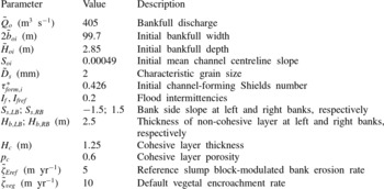
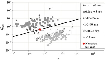
. The formative Shields number is estimated using the regression fit of Li et al. (Reference Li, Czapiga, Eke, Viparelli and Parker2014) which is as expressed in (3.10), and the corresponding bankfull channel characteristics are obtained from (3.7) to (3.9). Table 2 shows the adopted model input parameters corresponding to a nearly straight reach of the Pembina River. Comparing with the dataset of Parker et al. (Reference Parker, Wilcock, Paola, Dietrich and Pitlick2007) and Wilkerson & Parker (Reference Wilkerson and Parker2011) for river reaches covering a broad range of grain size classes, we see, as shown in figure 9, that the channel-forming Shields number
 ${\it\tau}_{form}^{\ast }$
corresponding to the model input parameters fits within the range for rivers of similar grain sizes. This value is used here as an initial value
 ${\it\tau}_{form,i}^{\ast }$
corresponding to a nearly straight or low-sinuosity channel.
Summary of input parameters for base run based on the Pembina River in Alberta, Canada. The subscript
 $i$
indicates initial values of parameters that change over time.

Channel forming (bankfull) Shields number versus channel slope
 $S$
. The datasets for bankfull geometry are from Parker et al. (Reference Parker, Wilcock, Paola, Dietrich and Pitlick2007) and Wilkerson & Parker (Reference Wilkerson and Parker2011). A point for the numerical test reach considered here, for which
 $\tilde{D}_{s}=2\ \text{mm}$
, has been added to the figure. Also shown is the line corresponding to (3.10) for
 $D=2\ \text{mm}$
.

The estimated reference erosional migration rate
 $\tilde{{\it\zeta}}_{Eref}=5\ \text{m}\ \text{yr}^{-1}$
is based on the following assumptions: an average cut bank 3.75 m high with a third of the bank height consisting of cohesive/rooted soil, a characteristic slump block size equal to the cohesive layer thickness, a reference slump block decay time
 $\tilde{T}_{cref}$
of 1.5 years, and a cohesive layer porosity
 $p_{c}=0.6$
. A default vegetal encroachment rate
 $\tilde{{\it\zeta}}_{veg}$
corresponding to approximately 10 % of initial bankfull width per year, or thus
 $10\ \text{m}\ \text{yr}^{-1}$
has been adopted. Here these numbers have been chosen in part by means of numerical experiments, so as to produce results that correspond to observations. In principle, all of these parameters are physically measurable, but measurement of
 $\tilde{T}_{cref}$
and
 $\tilde{{\it\zeta}}_{veg}$
in particular would require an extensive field campaign that is beyond the scope of this work.
For the initial low-amplitude channel, we assume an along-channel centreline wavelength
 $\tilde{{\it\lambda}}$
of 2 km and an initial maximum curvature value
 $c_{apex}={\it\upsilon}=0.025$
.
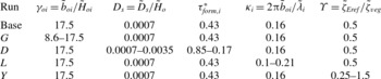
The input parameters shown in table 2 are for the base run. In addition to the base case, numerical experiments were carried out to determine model sensitivity to selected non-dimensional parameters. The input parameters for the various runs (Runs
 $G,D,L$
and
 $Y$
, as explained below) expressed in terms of dimensionless numbers are shown in table 3.
Input conditions for different numerical runs to find the effect of non-dimensional parameters on width curvature correlation. The subscript
 $i$
indicates initial values of parameters that change over time.

Going from left to right, the dimensionless parameters shown in each column are the half-width to depth ratio or aspect ratio
 ${\it\gamma}_{o}$
, the dimensionless grain size
 $D_{s}$
, the channel forming Shields number
 ${\it\tau}_{form}^{\ast }$
, the dimensionless channel wavenumber
 ${\it\kappa}$
and the ratio of reference erosion rate to reference deposition rate,
 ${\it\Upsilon}$
. The first four parameters are considered to be key governing parameters in river morphodynamics. The last parameter,
 ${\it\Upsilon}$
, specifically defined as
 $$\begin{eqnarray}{\it\Upsilon}=\frac{\tilde{{\it\zeta}}_{Eref}}{\tilde{{\it\zeta}}_{veg}}\end{eqnarray}$$
is here shown to be critical in determining the correlation between channel width and curvature. By varying discharge within the range of estimated bankfull discharge, i.e. from 200 to
 $405\ \text{m}^{3}\ \text{s}^{-1}$
, we vary the initial value of the aspect ratio from 8.6 to 17.5 in the
 $G$
runs. We vary both the grain size and formative Shields number in the
 $D$
runs by increasing the grain size from coarse sand to medium gravel, i.e. from 2 to 10 mm. Finally, we vary the reference migration parameter in runs
 $Y$
by fixing the reference erosion parameter
 $\tilde{{\it\zeta}}_{Eref}=5\ \text{m}\ \text{yr}^{-1}$
and varying the deposition parameter accordingly so that
 ${\it\Upsilon}$
varies from 0.25 to 1.5. As a check, the
 $Y$
runs were repeated for different values of
 $\tilde{{\it\zeta}}_{Eref}$
.
5.2. Constant versus slope-dependent channel-forming Shields number
We indicated in § 3 that the adoption of a constant value of channel-forming Shields number
 ${\it\tau}_{form}^{\ast }$
equal to the initial value
 ${\it\tau}_{form,i}^{\ast }$
leads to a channel that becomes unacceptably narrow as sinuosity increases. This point is illustrated in more detail in Eke (Reference Eke2013) and Eke et al. (Reference Eke, Parker and Shimizu2014). Here we illustrate this process, and also illustrate how the slope-dependent form (3.10) for channel-forming Shields number resolves this problem.
The calculation is first performed for the base case values under the assumption of constant
 ${\it\tau}_{form}^{\ast }=0.426$
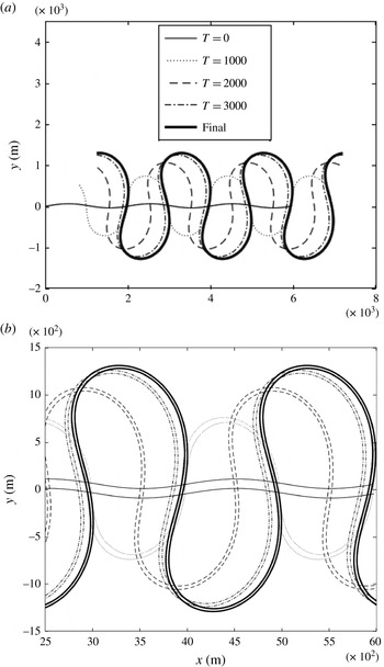
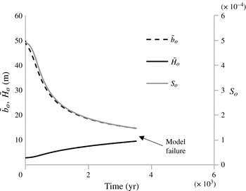
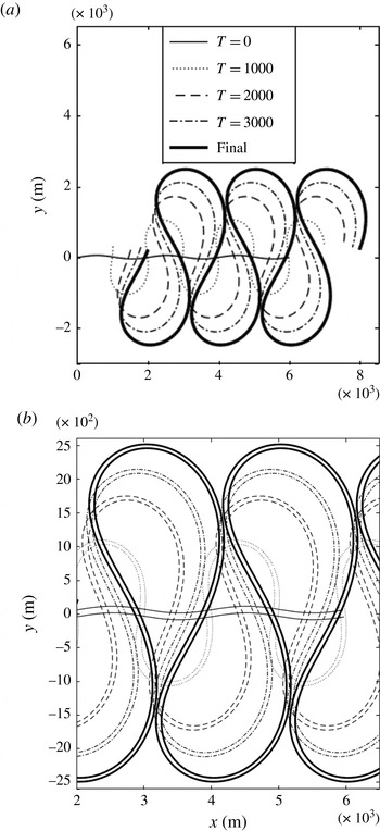
(table 2). Figure 10(a) shows the planimetric evolution of the channel centreline over time in terms of five snapshots from time
 $t=0$
, each at 1000-year intervals, and figure 10(b) plots the two banklines over the same time interval. In figure 10(a) we see that the channel undergoes an initial rapid downstream and lateral channel migration rate which reduces as the sinuosity increases. The figure also shows the development of an upstream skewing bias as the channel elongates (e.g. Parker et al., Reference Parker, Diplas and Akiyama1983). The simulation does not reach incipient cut-off, as the numerical model fails not long after the last snapshot at
 $t=3400\ \text{yr}$
. Figures 10(b) and 12 illustrates the cause of failure.
An example model simulation of an idealized periodic channel from an initial low amplitude to high amplitude, with constant channel-forming Shields number. (a) Centerline migration over time. (b) Planform showing evolution of channel width over time. Time indicated is in years.

The continuous variation of the downchannel slope triggered by planimetric evolution results in a variation of reach-averaged/reference channel characteristics. As shown in figures 10(b) and 11, with increasing sinuosity, channel width and depth adjust as expected. Mean bankfull width reduces and mean bankfull depth increases with the progressive decline in channel slope. The result is a channel that becomes progressively deeper and narrower as it approaches cut-off. This narrowing yields a width–depth ratio that is not only unrealistically small from a physical point of view, but also causes failure of the numerical model, as shown in figure 11.
Reference channel adjustment over time in response to increasing channel sinuosity. As slope
 $S_{o}$
reduces, the channel half-width
 $\tilde{b}_{o}$
reduces and flow depth
 $\tilde{H}_{o}$
increases. Model results assume a constant channel-forming Shields number.

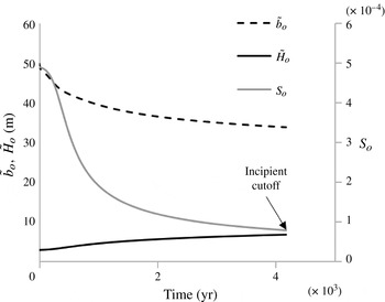
Figures 12 and 13 show the corresponding calculations for the case of a slope-dependent channel-forming Shields number varying according to (3.10). Although channel narrowing is observed, the channel continues to develop sinuosity until incipient neck cutoff. This result highlights the significance of the work of Li et al. (Reference Li, Czapiga, Eke, Viparelli and Parker2014), who demonstrate that bankfull Shields number increases to about the half power of channel slope. The model results show that the inclusion of this effect is important in the analysis of meandering channels with self-formed width.
An example model simulation of an idealized periodic channel from an initial low amplitude to high amplitude, with slope-dependent channel-forming Shields number. (a) Centerline migration over time. (b) Planform showing evolution of channel width over time. Time indicated is in years.

Reference channel adjustment over time in response to increasing channel sinuosity. As slope
 $S_{o}$
reduces, the channel half-width
 $\tilde{b}_{o}$
reduces and flow depth
 $\tilde{H}_{o}$
increases. Model results assume a slope-dependent channel-forming Shields number.

In all cases below, the channel-forming Shields number is assumed to be slope-dependent according to (3.10).
5.3. Base case
The planimetric evolution of the base simulation is as shown in figure 12. In addition to a migration rate and a mean channel width that declines, it can be discerned that the channel develops and maintains a spatial width variation pattern which becomes less prominent over time as the channel elongates. The nature of this variation is illustrated more clearly below.
Let
 $c_{apex}$
denote the dimensionless curvature at the bend apex,
 $\dot{{\tilde{n}}}_{max}$
denote the (dimensioned) magnitude of the maximum centreline lateral migration rate of the channel bend, and
 ${\it\delta}$
denote the (dimensionless) strength of the width variation deviation, here defined as
 $$\begin{eqnarray}{\it\delta}=\frac{\tilde{B}_{max}-\tilde{B}_{min}}{4\tilde{b}_{o}}\end{eqnarray}$$
where
 $\tilde{B}_{max}$
and
 $\tilde{B}_{min}$
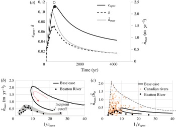
are the maximum and minimum widths for the reach at a given time. Over the course of channel evolution, we observe, as shown in figure 14(a), that
 $c_{apex}$
,
 ${\it\delta}$
and
 $\dot{{\tilde{n}}}_{max}$
rapidly increase, reach a peak value at 498, 450 and 425 years, respectively, and then decline more slowly. The peak values obtained for the migration rates and width variation are within the range of observed values for the reach of the Pembina River in question.
Channel evolution characteristics for the base run. (a) Variation of peak curvature
 $c_{apex}$
, centreline migration rate
 $\dot{{\tilde{n}}}_{max}$
and width variation amplitude
 ${\it\delta}$
over time (b) computed hysteresis loop for centreline migration rate. The arrow indicates direction of trajectory from low-amplitude meander to incipient cut-off. Also shown are data from the Beatton River, Canada (c) relation between migration rate and bend curvature, as well as 21 other Canadian rivers reaches (Hickin & Nanson Reference Hickin and Nanson1984).

In figure 14(b), the loop curve mapping the computed relationship between maximum migration rate
 $\dot{{\tilde{n}}}_{max}$
and dimensionless radius of curvature
 $1/c_{apex}$
up to incipient cutoff for the base case is shown. The peak migration rate shown on the loop falls toward the lower end of the observed range of peak values, i.e.
 $2{-}5\ \text{m}\ \text{yr}^{-1}$
reported by Beck et al. (Reference Beck, Harrington and Andres1983). Beck et al.’s values are for the relatively rapidly migrating Manola subreach rather than the entire reach of figure 2.
Also shown in figure 14(b) are data of Hickin & Nanson (Reference Hickin and Nanson1984) for the Beatton River, Canada. These are included only to illustrate a similar trend for sufficiently large radius of curvature; evidently the Beatton River has a peak migration rate that is substantially lower than the reach of the Pembina River studied here.
In figure 14(c), the computed loop curve in the form of
 $\dot{{\tilde{n}}}_{max}/\tilde{b}_{o}$
versus
 $1/c_{apex}$
is plotted against data for the Beatton River, as well as 21 other river reaches in Canada, including the Pembina River. Also shown in figure 14(c) is an envelope curve bounding the data from above. Figure 14(b,c) suggest model performance that is in the expected range for meandering rivers. The model does not capture a zone within which migration rate decreases with increasing curvature (decreasing radius of curvature
 $1/c_{max}$
). This may be due to (
 $a$
) limitations of the model at high curvature, or (
 $b$
) behaviour observed in the field associated with the development of bend complexity and cut-off (Hickin & Nanson Reference Hickin and Nanson1984; Hooke Reference Hooke2003). The observed behaviour at very high curvature is not captured in the simple implementation shown in figure 12, corresponding to a periodic bend developing only as far as cutoff, but can be partially captured in an implementation that includes non-periodicity and goes beyond cutoff (Eke Reference Eke2013).
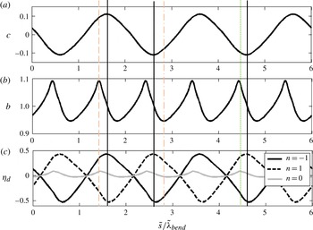
Figure 15 shows the downstream variation in dimensionless curvature
 $c$
, half-width
 $b$
and relative bed elevation
 ${\it\eta}_{d}$
at channel right, left and centre (i.e.
 $n=-1,1$
and 0, respectively) for the time
 $t=500\ \text{years}$
. This time is when the bends reach peak curvature, i.e. point O in figure 14(a). The downstream coordinate
 $\tilde{s}$
has been scaled by the bend length
 $\tilde{{\it\lambda}}_{bend}=\tilde{{\it\lambda}}/2$
.
Downstream variation in dimensionless curvature
 $c$
, half-width
 $b$
and relative bed elevation
 ${\it\eta}_{d}$
at time
 $t=498\ \text{yr}$
corresponding to peak bend amplitude (point O in figure 14
a). Continuous vertical lines indicate bend apex location, thin (red online) dashed lines indicate maximum width, thin (red online) dash-dotted lines indicate location of minimum width, and thin (green online) dotted lines indication location of maximum centreline bed elevation.

The width is shown to spatially oscillate at twice the wavelength of curvature. The bed elevation at the left and right banks shows a primary oscillation at the wavelength of curvature, but hidden in the variation is a second harmonic. This second harmonic, which appears only when nonlinear effects are included in the numerical model (§ 4.1), is readily seen in terms of centreline bed elevation, which, like width, oscillates at twice the wavelength of curvature. This prominent second harmonic at the channel centreline is present even for the case of a constant-width channel. It has been considered to be an indication of a tendency for central bars to emerge (Luchi et al. Reference Luchi, Zolezzi and Tubino2010) and has been used as a basis for the ‘curvature-forced’ mechanism for mid-channel bar development proposed by Luchi et al. (Reference Luchi, Zolezzi and Tubino2010).
Figure 15 shows that for the base run, the width maximum falls just upstream of the bend apex, and the minimum somewhat farther downstream of it. The bends of the Pembina do indeed show this behaviour, as can be seen in figure 7. The centreline bed elevation responds in kind with its peak located just upstream of the bend apex.
At this point it is useful to recall the analysis of field data in § 2, in which local dimensionless width
 $b$
is plotted against the absolute value of local dimensionless curvature
 $|c|$
(figures 4 and 5). In the field data, the width–curvature correlation over multiple bends appears as a series of scatter points to which we have fitted a regression line. Along one wavelength of a single bend, however, the correlation appears as a loop, with width varying with curvature along the bend. For the simplified case of a periodic channel, the result is a closed loop. Figure 16 shows this loop for the base case, at time
 $t=498\ \text{yr}$
. Also shown is the corresponding loop for deviatoric bed elevation along the centreline, denoted as
 ${\it\eta}_{C}$
, to distinguish it from the cross-sectionally averaged deviatoric bed elevation
 ${\it\eta}_{dc}$
. The arrows denote the path from the inflection point (where
 $c=0$
) downstream to the point of maximum curvature magnitude
 $|c|$
, and then farther downstream to the next inflection point.
Loop curves along a meander bend at
 $t=498\ \text{yr}$
for width
 $b$
and deviatoric centreline bed elevation
 ${\it\eta}_{C}$
as functions of the absolute value of curvature. The locations A, B, C and D correspond respectively to the inflection point, point of maximum width, point of maximum curvature and point of minimum width along the loop for
 $b$
. The points
 $\text{A}^{\prime },\text{B}^{\prime },\text{C}^{\prime }$
and
 $\text{D}^{\prime }$
correspond respectively to the inflection point, point of maximum deviatoric bed elevation, point of maximum curvature and point of minimum deviatoric bed elevation along the loop for
 ${\it\eta}_{C}$
. Arrows indicate direction of trajectory.

It is seen in the figure that width increases with increasing curvature downstream of the inflection point A, and reaches a maximum at point B, somewhat upstream of point C corresponding to the bend apex (maximum
 $|c|$
). Downstream of point B, width then decreases. At the bend apex, width differs little from the value at the inflection point. Farther downstream, width reaches a minimum at point D, located well downstream of the apex C. Width then increases from point D to point A, which now corresponds to the next inflection point downstream. Over time, this loop expands outwards during the growth phase of the planimetric evolution envelope and subsequently shrinks inward as incipient cutoff is reached.
The corresponding loop for deviatoric centreline bed elevation
 ${\it\eta}_{C}$
in figure 16 also shows an increase in bed elevation downstream of the inflection point
 $\text{A}^{\prime }$
to a maximum at
 $\text{B}^{\prime }$
, which is just downstream of the maximum in curvature B. Deviatoric centreline bed elevation then declines farther downstream, but is still well above zero at the bend apex
 $\text{C}^{\prime }$
. Minimum deviatoric centreline bed elevation continues to decline to point
 $\text{D}^{\prime }$
, located somewhat downstream of the point of minimum width D, and then increases back to point
 $\text{A}^{\prime }$
corresponding to the next inflection point downstream. The width at the apex is shown to be nearly the same as that at the crossing. Having said this, the point of width maximum is upstream of the apex, and closer to the apex than the nearest crossing, which is in line with the general trends observed in figure 7.
To show how correlation trends change over time as the bend develops toward incipient cutoff, let
 ${\it\phi}_{apex},{\it\phi}_{Bmax},{\it\phi}_{Bmin},{\it\phi}_{{\it\eta}cmax}$
denote the respective dimensionless phase distances, from an upstream inflection point to the location of the curvature maximum, width maximum, width minimum and centreline bed elevation maximum, respectively. The phase distance represents an arc length that has been rescaled by the channel bend length
 $\tilde{{\it\lambda}}_{bend}$
such that it ranges from 0 at the upstream inflection point to 1 at the downstream inflection point. The time variation of
 ${\it\phi}_{apex},{\it\phi}_{Bmax},{\it\phi}_{Bmin},{\it\phi}_{{\it\eta}cmax}$
is shown in figure 17(a). The figure also shows the phase distance to the location of maximum centreline migration rate
 ${\it\phi}_{M}$
.
Plots of time variation of normalized along-channel location of width maximum (
 ${\it\phi}_{Bmax}$
on the left,
 ${\it\omega}_{Bmax}$
on the right), maximum deviatoric centreline bed elevation (
 ${\it\phi}_{{\it\eta}cmax}$
on the left,
 ${\it\omega}_{{\it\eta}cmax}$
on the right), width minimum (
 ${\it\phi}_{Bmin}$
on the left,
 ${\it\omega}_{Bmin}$
on the right), maximum migration rate (
 ${\it\phi}_{M}$
on the left,
 ${\it\omega}_{M}$
on the right) and maximum curvature (bend apex:
 ${\it\phi}_{apex}$
on the left). (a) Variation of
 ${\it\phi}_{Bmax}$
,
 ${\it\phi}_{{\it\eta}cmax}\ {\it\phi}_{Bmin}$
,
 ${\it\phi}_{M}$
and
 ${\it\phi}_{apex}$
, representing phase position downstream of the inflection point. The (red online) dotted line indicates the bend geometric midpoint. (b) Variation of phase distances
 ${\it\omega}_{Bmax}$
,
 ${\it\omega}_{{\it\eta}cmax}\ {\it\omega}_{Bmin}$
and
 ${\it\omega}_{M}$
, normalized relative to the bend apex.

In figure 17(a), the point
 ${\it\phi}=0.5$
corresponds to half the distance from inflection point to the next inflection point downstream. Thus,
 $0<{\it\phi}<0.5$
corresponds to the upstream half of the bend, and
 $0.5<{\it\phi}<1$
corresponds to the downstream half. It is seen from the curve of
 ${\it\phi}_{apex}$
in the figure that the bend apex quickly moves into the upstream half of the bend, and stays there until incipient cutoff. This corresponds to bends that are skewed upstream (e.g. Parker et al.
Reference Parker, Diplas and Akiyama1983).
The curves of
 ${\it\phi}_{Bmax}$
and
 ${\it\phi}_{Bmin}$
in figure 18(a) indicate that maximum width is always attained upstream of the apex, and minimum width is always attained downstream of the apex. The bend apex always falls downstream of the point of maximum width and upstream of the point of minimum width, but is closer to the point of maximum width. The point of maximum width is always in the upstream half of the bend; this trajectory is also tracked by the phase location
 ${\it\phi}_{{\it\eta}cmax}$
corresponding to maximum deviatoric centreline bed elevation. The location of minimum width
 ${\it\phi}_{Bmin}$
shifts from the upstream half to the downstream half of the bend as the meander train evolves. The location of maximum migration rate
 ${\it\phi}_{M}$
tracks the location of minimum width.
Sensitivity of time trajectories of width variation intensity
 ${\it\delta}$
versus downchannel wavenumber
 ${\it\kappa}$
to variation in input parameters. (a) Sensitivity to aspect ratio
 ${\it\gamma}_{oi}$
. (b) Sensitivity to dimensionless grain size
 $D_{s}$
. (c) Sensitivity to initial wavenumber
 ${\it\kappa}_{i}$
. The thick lines indicate the base run and the straight arrows indicate the direction of increase. Temporal evolution along each curve is from right to left as indicated by the curved arrow in (a).

Another way to measure width–curvature–bed elevation phasing is to define the phase distance relative to the bend apex,
 ${\it\omega}$
, as
 $$\begin{eqnarray}{\it\omega}_{q}=\left\{\begin{array}{@{}ll@{}}\displaystyle \frac{{\it\phi}_{q}-{\it\phi}_{apex}}{{\it\phi}_{u}}\quad & {\it\phi}_{q}-{\it\phi}_{apex}<0\\ \displaystyle \frac{{\it\phi}_{q}-{\it\phi}_{apex}}{{\it\phi}_{d}}\quad & {\it\phi}_{q}-{\it\phi}_{apex}>0\end{array}\right.\end{eqnarray}$$
where
 $q$
is a given variable (e.g.
 $q={\it\eta}_{dc}$
for deviatoric centreline bed elevation) and
 ${\it\phi}_{u}$
and
 ${\it\phi}_{d}$
denote the upstream and downstream phase distance relative to the bend apex as defined in figure 17(a), so that the two sum to unity. The parameter
 ${\it\omega}_{q}$
is thus defined such that it varies from
 $-$
1 to 1 with 0 corresponding to the bend apex and
 $-$
1 and 1 corresponding to the upstream and downstream inflection points, respectively. The variations over time of location of the width maximum
 ${\it\omega}_{Bmax}$
, width minimum
 ${\it\omega}_{Bmin}$
, maximum deviatoric centreline bed elevation
 ${\it\omega}_{{\it\eta}cmax}$
and maximum migration rate
 ${\it\omega}_{M}$
are shown in figure 17(b). In the figure we see that over time, the normalized locations of the width maximum and deviatoric central bed elevation maximum remain fairly constant at approximately
 ${\it\omega}=-0.3$
. The locations of the width minimum and maximum migration rate, on the other hand, shows significant change during bend development, but eventually approach an asymptote of
 ${\it\omega}=0.25$
up to incipient cutoff.
5.4. Model sensitivity to channel parameters
Changes to the aspect ratio, grain size and initial wavelength were found to alter the lateral migration rates predicted by the model. For example, a reduction in the initial aspect ratio
 ${\it\gamma}_{oi}$
from the base value was found to result in lower curvature peaks as well as reduced channel migration rates. Increased sediment size also resulted in a decrease in migration rates. Increasing the initial channel wavenumber
 ${\it\kappa}$
(i.e. decreasing the wavelength) from the base value, however, was found to increase the migration rate and yield a higher curvature peak. These tendencies were computed by performing the
 $G$
runs (variation in
 ${\it\gamma}_{oi}$
),
 $D$
runs (variation in
 $D_{s}$
) and
 $L$
runs (variation in
 ${\it\kappa}$
) of table 3. The results are summarized in figure 18.
Figure 18(a–c) all show time trajectories of width variation intensity
 ${\it\delta}$
versus down-channel meander wavenumber
 ${\it\kappa}$
. In all cases temporal variation is from right to left, as indicated by the curved arrow in figure 18(a). The sensitivity of this trajectory to variation in initial aspect ratio
 ${\it\gamma}_{oi}$
is shown in figure 18(a); the sensitivity to varied dimensionless grain size
 $D_{s}$
is shown in figure 18(b), and the sensitivity for varied initial wavenumber
 ${\it\kappa}_{i}$
is shown in figure 18(c). The base case is shown as the thick black line for each figure. The straight arrow denotes the direction of increase of the parameter in question.
For each case, as the channel evolves over time, the channel wavenumber steadily drops, corresponding to increasing sinuosity. As time passes and wavenumber drops, the intensity of width variation increases, reaches a peak, and then declines. The magnitude of this peak evidently increases with increasing initial aspect ratio
 ${\it\gamma}_{oi}$
and initial wavenumber
 ${\it\kappa}_{i}$
. Although the behaviour is less consistent in terms of grain size, a grain size that is five times the base value results in a near-doubling of width variation intensity.
The phasing of width oscillation with respect to curvature is also impacted by changes to the parameters
 ${\it\gamma}_{oi},D_{s}$
and
 ${\it\kappa}_{i}$
. This sensitivity is illustrated in terms of the time trajectories of
 ${\it\omega}_{Bmax}$
and
 ${\it\omega}_{Bmin}$
versus
 ${\it\kappa}$
given in figure 19(a–c). In all cases temporal evolution is from right to left, i.e. the direction of increasing wavenumber
 ${\it\kappa}$
. The general trend is for the location of the width minimum to be shifted upstream toward the bend apex as sinuosity increases over time. This is seen in all cases shown in figure 19. The width minimum shifts upstream for increasing
 ${\it\gamma}_{oi}$
and downstream for increasing grain size. The location of the width maximum is largely unaffected by
 ${\it\gamma}_{oi}$
, but shows a significant downstream shift toward the bend apex for larger grain sizes.
Sensitivity of time trajectories of normalized phase relative to bend apex
 ${\it\omega}_{Bmax}\ {\it\omega}_{Bmin}$
, corresponding to maximum and minimum width versus downchannel wavenumber
 ${\it\kappa}$
, to variation in input parameters. (a) Sensitivity to aspect ratio
 ${\it\gamma}_{oi}$
. (b) Sensitivity to dimensionless grain size
 $D_{s}$
. (c) Sensitivity to initial wavenumber
 ${\it\kappa}_{i}$
. The thick lines indicate the base run and the straight arrows indicate the direction of increase. Temporal evolution along each curve is from right to left. The values of
 ${\it\gamma}_{oi},D_{s}$
and
 ${\it\kappa}_{I}$
are the same as in figure 18.

In all of the above simulations shown, while the width–curvature trajectory is seen to change with changing input parameters, the general tendency is for the width maximum to be located just upstream of the bend apex and for the minimum to be located slightly to significantly downstream. In the next section, however, we show that this pattern is a strong function of the reference erosion and deposition rates. We study this by varying their ratio (
 $Y$
runs of table 3).
5.5. Model sensitivity to bank parameters
Figure 20 shows results for bed topography and bank lines obtained from model simulations from the
 $Y$
runs of table 3, where the ratio of the reference erosion rate to reference deposition rate
 ${\it\Upsilon}=\tilde{{\it\zeta}}_{Eref}/\tilde{{\it\zeta}}_{veg}$
is varied by holding the erosion rate
 $\tilde{{\it\zeta}}_{Eref}$
constant and varying the deposition rate
 $\tilde{{\it\zeta}}_{veg}$
accordingly. More specifically in addition to the base value
 ${\it\Upsilon}=0.5$
, the values 0.25, 0.75, 1.0, 1.25 and 1.5 are also considered. Again each snapshot shown here represents the time at which curvature reaches the peak of its envelope curve (e.g. figure 15
a). The values of the peak curvature and migration rates for each of the snapshots are indicated in the figure.
Plots of bed topography contours and bank lines illustrating sensitivity variation in the coefficient
 ${\it\Upsilon}=\tilde{{\it\zeta}}_{Eref}/\tilde{{\it\zeta}}_{veg}$
. In the plots,
 $\tilde{{\it\zeta}}_{Eref}$
is held constant at
 $5\ \text{m}\ \text{yr}^{-1}$
while
 $\tilde{{\it\zeta}}_{veg}$
is reduced from (a)–(f), so yielding the increasing values of
 ${\it\Upsilon}$
. The bank lines correspond to the bounds of the bank region of figure 8. Each plots correspond to the time at which peak bend amplitude was reached. Direction of flow is from left to right in all cases. The filled and white arrows correspond to the location of maximum and minimum width for
 ${\it\Upsilon}=0.25$
, respectively. Width deviation has been magnified by 5 for visualization.

In the figures, the bank lines correspond to the bounds of the central region of figure 8. The contour lines shown indicate dimensionless relative bed elevation. The near-zero contour of 0.05 has been highlighted to better visualize the point bar configuration in each plot. Here we define the point bar in terms of the portion of the channel between the 0.05 contour and the lower bank in the plot.
Figure 20(a–f) show a steady progression in pattern as
 ${\it\Upsilon}$
increases. This is most readily seen in terms of the two points, A and B, in figure 20(a). Point A, marked with a solid arrow, shows the position of maximum width for
 ${\it\Upsilon}=0.25$
, and point B, marked with an open arrow, shows the position of minimum width for the same value of
 ${\it\Upsilon}$
. These same positions are marked with corresponding solid and open arrows for the cases
 ${\it\Upsilon}=0.50$
, 0.75, 1.0, 1.25 and 1.5 in figure 20(b–f), respectively. The width at the point of the solid arrow monotonically decreases with increasing
 ${\it\Upsilon}$
, so that the point becomes very nearly the narrowest point on the bend for
 ${\it\Upsilon}=1.50$
. The width at the point of the open arrow monotonically increases with increasing
 ${\it\Upsilon}$
, so that this point is not too far from the width maximum at
 ${\it\Upsilon}=1.5$
. The systematic variation of width at the points of the solid and open arrows is illustrated in figure 20.
It can also be seen that as
 ${\it\Upsilon}$
increases from 0.25 to 1.50, the intensity of width variation first decreases, and then increases. A corresponding pattern can be seen somewhat downstream of the bend apex at point ‘B’, with monotonically increasing width as
 ${\it\Upsilon}$
increases from 0.25 to 1.50. The value of the dimensionless width at point A and B for each of the cases shown in figure 20 are plotted as a function of
 ${\it\Upsilon}$
in figure 21.
Dimensionless half-width at a fixed point A upstream of the bend apex and a fixed point B downstream of the bend apex as a function of
 ${\it\Upsilon}$
. The positions of these points are depicted in figure 21. The values for
 ${\it\Upsilon}=0.25$
correspond to maximum width (A) and minimum width (B).

The case
 ${\it\Upsilon}=0.5$
shown in figure 20(b) is of particular interest because it corresponds to the base case. It is seen from the figure that the model predicts a point of maximum width that lies upstream of the bend apex just as seen in the field.
The teardrop shape of the point bar delineated by the 0.05 bed elevation contour line also undergoes a systematic transition as
 ${\it\Upsilon}$
increases, with the locus of maximum bar width moving from upstream of the bend apex to downstream of it.
This systematic change in the pattern of width variation with increasing
 ${\it\Upsilon}$
may be one reason why each of the four field cases shown in figures 4 and 5 shows a different relation for
 $b$
versus
 $|c|$
.
Bend migration patterns can be characterized in terms of ‘bank pull’ and ‘bar push’. Based on Stillwater Science (2007), Eke et al. (Reference Eke, Parker and Shimizu2014) defined these as follows: a cross-section is undergoing bank pull when the eroding bank is migrating faster than the depositing bank, and it undergoes bar push when the depositing bank is migrating faster than the eroding bank. Stillwater Science (2007) relates these modes of migration to the effect of topographic steering of the flow by the point bar.
It might be thought that an increase in
 ${\it\Upsilon}=\tilde{{\it\zeta}}_{Eref}/\tilde{{\it\zeta}}_{veg}$
would engender an across-the-board increase in erosion-dominated migration (bank pull) over deposition-dominated migration (bar push). The behaviour predicted by the model is at variance with this. In the present model, the overall migration pattern tends to be predominantly deposition-dominated, due to the net reduction in channel width over time documented in figure 13. However, within the channel itself, it has been observed that there is a spatial distribution of patterns of bank pull and bar push. These have been documented through field and experimental observation to correlate with the location of the point bar (Stillwater Science 2007).
Figure 22 shows the centreline curvature distribution for cases corresponding to
 ${\it\Upsilon}=0.25$
, 0.5, 1.25 and 1.5 in figure 20. The shaded regions indicates zones where bank pull is the dominant channel migration mechanism. Regions without shading are dominated by bar push.
Plots showing centreline curvature versus normalized streamwise distance for the values
 ${\it\Upsilon}=0.25$
, 0.5, 1.25 and 1.50 (a–d). The run conditions correspond to those of figure 20. Zones of bank pull are marked with shaded regions; the absence of which implies bar push.

As shown in figure 22, bank-pull zones are found just downstream of the bend apex, for lower values of
 ${\it\Upsilon}$
. As
 ${\it\Upsilon}$
increases, these zones migrate upstream, even as the location of the width maximum, as documented in figure 20, migrates downstream. Figures 20 and 22 present a consistent picture of the effect of topographic steering in meander bends. The presence of significant width variation and the accompanying enlarged point bar upstream of the bend apex steers flow toward the outer bank upstream, causing an elevated erosion rate at or downstream of the bend apex. Thus, as the width maximum shifts downstream towards the infection point, the zone of elevated erosion rates shifts accordingly.
In figure 23, width
 $b$
, centreline bed elevation,
 ${\it\eta}_{C}$
and centreline water surface elevation
 ${\it\xi}_{C}$
are plotted against curvature magnitude
 $|c|$
for the cases
 ${\it\Upsilon}=0.25$
, 0.75 and 1.5 of the
 ${\it\Upsilon}$
runs of table 3. This figure documents a transition from a generally positive correlation between width and curvature for
 ${\it\Upsilon}=0.25$
to a generally negative one for
 ${\it\Upsilon}=1.25$
, similar to the transition observed in the field data comparison between the Vermillion River and Trinity River Reaches in § 2. This suggests that the present model can encompass the full range of trends documented in figures 4 and 5, including the positively correlated case of the Trinity River and the negatively correlated case of the Vermillion River.
Loop curves along a meander bend at the time of maximum apex curvature for width
 $b$
, deviatoric centreline bed elevation
 ${\it\eta}_{C}$
and deviatoric centreline water surface elevation
 ${\it\xi}_{C}$
as functions of the absolute value of curvature. Results for the four cases (a–d)
 ${\it\Upsilon}=$
0.25, 0.5, 0.75 and 1.5 are shown; the base case corresponds to
 ${\it\Upsilon}=0.5$
. Straight lines indicate the linear regression fit for width and absolute curvature. Arrows indicate direction of trajectory.

The case of figure 23(b) is of particular interest, because it corresponds to the base case
 ${\it\Upsilon}=0.5$
for the Pembina River. The predicted trend is for width to be positively correlated with the magnitude of curvature, as is indeed the case for the Trinity River in figure 4.
Figure 23 also shows that the magnitude of the deviatoric centreline bed oscillation
 ${\it\eta}_{C}$
varies with the intensity of width variation. For the cases
 ${\it\Upsilon}=0.25$
and
 ${\it\Upsilon}=1.5$
, corresponding to significant width variation, the values of
 ${\it\eta}_{C}$
are significantly greater than for the
 ${\it\Upsilon}=0.75$
, corresponding to very little width variation.
The above result (figures 16 and 23) is significant in the light of the recent work of Luchi et al. (Reference Luchi, Bolla Pittaluga and Seminara2012) where an analytical model was developed to predict channel width variation for the equilibrium river. They hypothesized that the width variation observed in an equilibrium channel should correspond to the one that yields the least streamwise variation in centreline water surface elevation
 ${\it\xi}_{C}$
, and thus the most nearly streamwise-constant water surface slope. They furthermore showed that this constraint results in a pattern of width variation such that width is maximum close to the crossings. Here, however, we find that the predicted pattern of width oscillation is not necessarily associated with, nor does it require, any tendency toward constant centreline water surface slope. Rather, the patterns of spatial variation of width, centreline bed elevation and centreline water surface elevation are functions of (among other things) the dimensionless parameter
 ${\it\Upsilon}$
corresponding to the reference erosion rate divided by the reference deposition rate.
6. Discussion
The model presented above has at least three limitations. First, it is applicable only to bedload-dominated rivers. In order to extend it to suspension-dominated rivers, the sediment transport needs to be reformulated so as to (a) divide bed material load into bedload and suspended load, (b) apply separate transport equations and (c) calculate transverse load under the influence of gravity solely from bedload.
Second, the model cannot capture the formation and migration of free bars (e.g. Seminara Reference Seminara2006). This is because it uses a specific variant of quasi-steady assumption; the characteristic time for planform adjustment is assumed to be sufficiently long compared with bed adjustment so as to allow a steady-state solution for bed morphology. The model of Asahi et al. (Reference Asahi, Shimizu, Nelson and Parker2013) discussed below is not subject to this constraint.
Third, the model captures only one type of natural armouring, i.e. slump blocks. In some cases, induration of otherwise non-cohesive floodplain sediment may act to throttle bank erosion below its default non-cohesive value. In relatively large streams, fallen trees and tree stumps may be more effective units of natural armouring than slump blocks (Konsoer et al. Reference Konsoer, Rhoads, Langendoen, Johnson and Ursic2012; Konsoer Reference Konsoer2014).
Having said this, the parameters entering into the submodels for bank erosion and deposition are all physically measurable quantities. More specifically,
 $\tilde{{\it\zeta}}_{veg}$
is the default rate of vegetal encroachment in the absence of near-bank shear stress long enough to limit it,
 $\tilde{H}_{c}$
is the characteristic thickness of the cut bank cohesive layer,
 $\tilde{D}_{c}$
is the characteristic size of the slump blocks and
 $\tilde{T}_{c}$
is the characteristic residence time of slump blocks are all measurable in the field. The model assumes fairly simple relations for the way in which deposition rate
 $\tilde{{\it\zeta}}_{D}$
decreases, and erosion rate
 $\tilde{{\it\zeta}}_{E}$
increases, with increasing near-bank Shields number. These relations can be refined as more field data become available.
The model presented here merits comparison with that of Asahi et al. (Reference Asahi, Shimizu, Nelson and Parker2013). An advantage of the model of Asahi et al. (Reference Asahi, Shimizu, Nelson and Parker2013) compared with the present one is that it encompasses free bars, and thus leads to a rather more complex pattern than that observed here. A disadvantage is that their model cannot yet be applied at field scale, whereas the present model has been applied using input values from the meandering Pembina River, Alberta, Canada. In addition, the model of Asahi et al. cannot be applied to width evolution in straight reaches, and thus is not yet able to fully describe how average width is maintained in meandering rivers. All of these limitations could be overcome by means of a future amalgamation of the two models.
The treatment of Asahi et al. (Reference Asahi, Shimizu, Nelson and Parker2013) for bank erosion is similar to that used here. The treatment of bank deposition, however, is different. The present analysis assumes a default rate of deposition associated with unrestricted vegetal encroachment, which is then reduced as near-bank bed shear stress during floods is increased. Asahi et al. (a) assume a two-step hydrograph, and (b) assign a characteristic time
 $T_{land}$
for exposed point bar to become stabilized by vegetation. Once a zone of the bed has been exposed for this time, it is stabilized, and is no longer a part of the riverbed. The only way the material can be removed is the river later erodes into it. For the same flood return period, larger values of
 $T_{land}$
result in wider channels, due the decreasing effectiveness of vegetal stabilization.
In the present analysis, flow hydrograph is not explicitly modelled. Instead, it is implicitly modelled via the forms (4.37) and (5.2) for the bank erosion rate and deposition rate, respectively. The former is proportional to flood intermittency
 $I_{f}$
, so that longer flood flows yield higher erosion rates. The latter is proportional to the fraction of time
 $(1-I_{f})$
corresponding to low flow, but decreases with increasing near-bank bed shear stress during floods, when vegetation can be partially or completely uprooted.
One way to bring the models into closer accord is the addition of a time lag effect in (5.2), so that
 $$\begin{eqnarray}\tilde{{\it\zeta}}_{D}=\tilde{{\it\zeta}}_{veg}\left[\left(1-I_{f}\right)-I_{lag}\right]\left(1-\frac{{\it\tau}_{D}^{\ast }}{{\it\tau}_{form}^{\ast }}\right).\end{eqnarray}$$
Here
 $I_{lag}$
corresponds to a fraction of the low-flow period necessary for the vegetation to take root. Larger values of
 $I_{lag}$
might correspond to vegetation types that take longer to become established, or coarser point bar sediment which inhibits establishment.
One more limitation of both this model and that of Asahi et al. (Reference Asahi, Shimizu, Nelson and Parker2013) is that while they can erode floodplain, they cannot build floodplain above the top of the point bar. The formulation of morphodynamic models of meandering rivers will not be complete until the floodplain, as well as the channel is self-formed. A basis for the formulation of a model that accounts for both the channel sediment material gained from channel erosion and that lost as the channel deposits and builds its floodplain can be found in Lauer & Parker (Reference Lauer and Parker2008).
The present model does not predict an ideal equilibrium for meandering channels. Instead, meanders develop to cutoff. In the present model, the cross-sectionally averaged sediment transport rate decreases in time as sinuosity increases, and thus mean slope decreases. In a long-term implementation of our model, the equilibrium state would be statistical, with a local increase of the sediment transport rate due to cutoffs. Frascati & Lanzoni (Reference Frascati and Lanzoni2009) offer a model that can capture this statistical equilibrium, albeit not with a self-formed width.
7. Conclusions
A large body of research on the theoretical and numerical simulation of the migration of meandering rivers is based on the HIPS model (Hasegawa Reference Hasegawa1977; Ikeda et al. Reference Ikeda, Parker and Sawai1981). This formulation assumes that the river maintains a constant, prescribed width as it migrates. Since the time of that research, however, it has been shown that meandering rivers show systematic spatial patterns of width variation (Brice Reference Brice1982; Lagasse et al. Reference Lagasse, Spitz, Zevenbergen and Zachmann2004).
We have used field data from five river reaches to demonstrate the existence of a range of patterns of spatial variation of width in meandering rivers. One end member is the case of the Trinity River, Texas, USA, where width shows strong positive correlation with the absolute value of centreline curvature. In this case, points near apexes tend to be wider than points near crossings. The other end member is the case of the Vermillion River, Minnesota, USA, where width shows weak negative correlation with curvature. In the case of the Suwannee and Apalachicola Rivers, Florida, USA and the Pembina River, Alberta, Canada, maximum width tends to occur upstream of the bend apex, whereas in Trinity River, maximum width tends to occur downstream of the bend apex, and in the case of the Vermillion River, both cases are equally likely.
We have invoked a physically based numerical model for self-formed, coevolving channel planform and width variation to study the underlying causes for these patterns. Our model uses the framework of Parker et al. (Reference Parker, Shimizu, Wilkerson, Eke, Abad, Lauer, Paola, Dietrich and Voller2011), applied to a stream for which bedload is the dominant mode of sediment transport. More specifically, it uses the submodels given in Eke et al. (Reference Eke, Parker and Shimizu2014) for bank erosion and deposition. In the case of an eroding bank, slump block armouring acts to hold the bank erosion rate well below the value that would prevail in the case of purely non-cohesive material. In the case of a depositing bank, vegetal encroachment stabilizes otherwise loose point bar sediment, causing the bankline to advance. As opposed to the earlier HIPS model of meander migration (Hasegawa Reference Hasegawa1977; Ikeda et al. Reference Ikeda, Parker and Sawai1981), all of the input parameters pertain to physical quantities in the two submodels are at least potentially measurable in the field.
A model that predicts width variation must also be capable of predicting overall mean width as well. This is accomplished in terms of three relations: a relation for momentum balance, a relation for bedload transport and a relation for channel-forming (bankfull) Shields number. In previous implementations of this formulation (e.g. Parker et al. Reference Parker, Paola, Whipple and Mohrig1998), channel-forming Shields number has been taken to be a prescribed constant. The resulting relations predict a bankfull width that varies inversely with bed slope. Here we have shown that as sinuosity increases, and thus mean down-channel bed slope decreases, such a relation applied to meandering streams predicts a drastic decrease in bankfull width. Li et al. (Reference Li, Czapiga, Eke, Viparelli and Parker2014) have shown, however, that bankfull Shields number is an increasing function of slope. We show here that this formulation overcomes the problem of over-narrowing; bankfull width decreases only mildly as sinuosity increases.
The following two parameters play key roles; the default rate of migration of a depositing bank,
 $\tilde{{\it\zeta}}_{veg}$
due to vegetal encroachment in the absence of flood flow, and a reference rate of migration of an eroding bank
 $\tilde{{\it\zeta}}_{Eref}$
that corresponds to a near-bank bed shear stress that is twice the bankfull value. In applying our model to a reach of the Pembina River we find that the dimensionless parameter
 ${\it\Upsilon}=\tilde{{\it\zeta}}_{Eref}/\tilde{{\it\zeta}}_{veg}$
controls the mode of spatial width variation. As
 ${\it\Upsilon}$
increases from 0.25 to 1.5, (a) the point of maximum width shifts from a position upstream of the apex to a position downstream of it, (b) the correlation between width and the magnitude of curvature shifts from positive to negative and (c) the locus of bank pull migrates from downstream of the apex to upstream of it. The case of least width variation is seen when
 ${\it\Upsilon}$
is near the intermediate value 0.75.
The predictions thus span the patterns of variation observed across the five field examples. It is not possible to compare the results directly to each of the five field examples, because the applicable input parameters are likely to be different from reach to reach. The predictions for the base case
 ${\it\Upsilon}=0.5$
of the Pembina River are, however, in agreement with the trends in the observations: width correlates positively with the absolute value of curvature, and the position of the width maximum is located upstream of the bend apex. A more detailed comparison awaits a more complete set of field data.
It should be borne in mind that the results presented here apply only to periodic trains of meanders. These trains begin as sine-generated curves, but evolve to periodic forms that deviate from the sine generated form. The case of bends evolving from randomly varying curvature is presented by Eke (Reference Eke2013).
The model for meander evolution presented here does not necessarily render the HIPS formulation obsolete. In the case
 ${\it\Upsilon}=0.75$
, for example, width variation is predicted to be modest. There may be a range of conditions for which the results of the present model for planform evolution do not differ too much from a parallel HIPS implementation with appropriately chosen input parameters. Such a parallel implementation and comparison should be a goal of future research.
Acknowledgements
This research represents a contribution of the National Center for Earth-surface Dynamics, a Science and Technology Center funded by the US National Science Foundation (agreement EAR-0120914). We thank R. Luchi for valuable advice on the research and the text.
Appendix A. ‘D’ solutions
Integrating the continuity equation (4.4) from the left bank
 $n=-1$
to
 $n$
subject to the boundary conditions in (4.15), we get the following solution for the transverse velocity in integral form, i.e.
 $$\begin{eqnarray}v_{d}=-\frac{\partial b_{d}}{\partial s}-\left(n+1\right)\left(\frac{\partial u_{dc}}{\partial s}+\frac{\partial {\it\xi}_{dc}}{\partial s}-\frac{\partial {\it\eta}_{dc}}{\partial s}\right)-\frac{\partial }{\partial s}\int _{-1}^{n}\left(u_{dd}+h_{dd}\right)\,\text{d}n^{\prime }+R_{1}\end{eqnarray}$$
where
 $$\begin{eqnarray}\displaystyle R_{1} & = & \displaystyle -\frac{\partial }{\partial s}\int _{-1}^{n}\left(h_{do}+{\it\xi}_{d}-{\it\eta}_{d}\right)\left(u_{do}+u_{d}\right)\text{d}n^{\prime }-v_{d}\left[h_{do}+{\it\xi}_{d}-{\it\eta}_{d}+nbcH\right]\nonumber\\ \displaystyle & & \displaystyle -\,\frac{\partial }{\partial s}b_{d}\int _{-1}^{n}\left(\left(u_{do}+u_{d}\right)H+h_{do}+{\it\xi}_{d}-{\it\eta}_{d}\right)\text{d}n^{\prime }\nonumber\\ \displaystyle & & \displaystyle +\,n\left(\left(u_{do}+u_{d}\right)H+h_{do}+{\it\xi}_{d}-{\it\eta}_{d}\right)\frac{\text{d}b_{d}}{\text{d}s}.\end{eqnarray}$$
The streamwise momentum equation (4.4) can be rewritten as follows:
 $$\begin{eqnarray}\displaystyle & & \displaystyle \frac{\partial \left(u_{dd}+u_{dc}\right)}{\partial s}+2{\it\varepsilon}\left(u_{do}+u_{dd}+u_{dc}\right)-{\it\varepsilon}\left(h_{do}+{\it\xi}_{dc}+{\it\xi}_{dd}-{\it\eta}_{dc}-{\it\eta}_{dd}\right)\nonumber\\ \displaystyle & & \displaystyle \qquad -\,{\it\varepsilon}S_{do}+F_{o}^{-2}\frac{\partial \left({\it\xi}_{dd}+{\it\xi}_{dc}\right)}{\partial s}+{\it\varepsilon}nC=R_{2}\end{eqnarray}$$
where
 ${\it\varepsilon}={\it\gamma}_{o}C_{f}$
and
 $$\begin{eqnarray}\displaystyle R_{2} & = & \displaystyle {\it\varepsilon}\left(1+b_{d}S_{do}\right)-\frac{v_{d}}{N}\frac{\partial u_{dd}}{\partial n}-U\left(b_{d}\frac{\partial \left(u_{dc}+u_{dd}\right)}{\partial s}-n\frac{\text{d}b_{d}}{\text{d}s}\frac{\partial u_{dd}}{\partial n}\right)\nonumber\\ \displaystyle & & \displaystyle -\,\left(u_{do}+u_{dc}+u_{dd}\right)\frac{\partial \left(u_{dc}+u_{dd}\right)}{\partial s}-bcU\left(v_{d}+2{\it\varphi}\right)\nonumber\\ \displaystyle & & \displaystyle -\,\frac{1}{HN}\frac{\partial HU{\it\varphi}}{\partial n}-F_{o}^{-2}\left(b_{d}\frac{\partial \left({\it\xi}_{dd}+{\it\xi}_{dc}\right)}{\partial s}-n\frac{\partial b_{d}}{\partial s}\frac{\partial {\it\xi}_{dd}}{\partial n}\right)-b{\it\gamma}_{o}\frac{{\it\tau}_{n}}{HN}\nonumber\\ \displaystyle & & \displaystyle +\,{\it\varepsilon}\left[2\left(u_{do}+u_{dc}+u_{dd}\right)-\left(h_{do}+{\it\xi}_{dc}+{\it\xi}_{dd}-{\it\eta}_{dc}+{\it\eta}_{dd}\right)+nc+b_{d}\right].\end{eqnarray}$$
Integrating (A 3) from the left bank to the right bank, we get
 $$\begin{eqnarray}\frac{\partial u_{dc}}{\partial s}-{\it\varepsilon}S_{do}+2{\it\varepsilon}\left(u_{do}+u_{dc}\right)-{\it\varepsilon}\left(h_{do}+{\it\xi}_{dc}-{\it\eta}_{dc}\right)+F_{o}^{-2}\frac{\partial {\it\xi}_{dc}}{\partial s}=R_{21}\end{eqnarray}$$
where
 $$\begin{eqnarray}R_{21}=\frac{1}{2}\int _{-1}^{1}R_{2}\text{d}n.\end{eqnarray}$$
Further integrating (A 5) in the streamwise direction from 0 to
 $L$
, we get
 $$\begin{eqnarray}-S_{do}+2u_{do}-h_{do}=R_{22}\end{eqnarray}$$
where
 $$\begin{eqnarray}R_{22}=\frac{1}{{\it\varepsilon}L}\int _{o}^{L}R_{21}\text{d}s.\end{eqnarray}$$
Thus, the solution to the ‘D’ components of the streamwise velocity is obtained in integral form by subtracting (A 5) from (A 3), i.e.
 $$\begin{eqnarray}u_{dd}=u_{dd}(0,n)\text{e}^{-2{\it\varepsilon}s}+\text{e}^{-2{\it\varepsilon}s}\int _{o}^{s}\text{e}^{2{\it\varepsilon}s}\left[{\it\varepsilon}{\it\xi}_{dd}-{\it\eta}_{dd}-F_{o}^{-2}\frac{\partial {\it\xi}_{dd}}{\partial s}-{\it\varepsilon}nc+R_{23}\right]\text{d}s^{\prime }\end{eqnarray}$$
where the periodic upstream boundary condition in (A 9) is given as
 $$\begin{eqnarray}u_{dd}(0,n)=\frac{1}{\left(\text{e}^{2{\it\varepsilon}L}-1\right)}\int _{o}^{L}\text{e}^{2{\it\varepsilon}s}\left[{\it\xi}_{dd}-{\it\eta}_{dd}-nc-F_{o}^{-2}\frac{\partial {\it\xi}_{dd}}{\partial s}+R_{23}\right]\text{d}s^{\prime }.\end{eqnarray}$$
In the above relation,
 $$\begin{eqnarray}R_{23}=R_{2}-\frac{1}{2}\int _{-1}^{1}R_{2}\text{d}n.\end{eqnarray}$$
From (4.6) we get the solution for the ‘D’ component of the water surface elevation, i.e.
 $$\begin{eqnarray}{\it\xi}_{dd}=F_{o}^{2}cn-F_{o}^{2}\int _{-1}^{n}R_{3}\text{d}n^{\prime }+F_{o}^{2}\frac{1}{2}\int _{-1}^{1}\int _{-1}^{n}R_{3}\text{d}n^{\prime }\text{d}n^{\prime \prime }\end{eqnarray}$$
where
 $$\begin{eqnarray}\displaystyle R_{3} & = & \displaystyle -v_{d}\frac{\partial v_{d}}{\partial n}-UbL_{sn}\left(V\right)-\frac{1}{H}bL_{sn}\left(UH{\it\varphi}\right)-cNb\left(2v_{d}{\it\varphi}+{\it\psi}-U^{2}\right)+c\nonumber\\ \displaystyle & & \displaystyle -\,2\frac{1}{H}\frac{\partial HV{\it\varphi}}{\partial n}-\frac{1}{H}\frac{\partial H{\it\psi}}{\partial n}-b\frac{{\it\gamma}_{o}{\it\tau}_{n}}{H}.\end{eqnarray}$$
Finally, the ‘D’ solution for the bed elevation perturbation is obtained from (4.9), i.e.
 $$\begin{eqnarray}\displaystyle {\it\eta}_{dd} & = & \displaystyle \frac{{\it\gamma}_{o}\sqrt{{\it\tau}_{so}^{\ast }}}{r}\left[\left(\frac{\partial b_{d}}{\partial s}+\frac{G(0)}{{\it\chi}{\it\varepsilon}}c\right)n+\int _{-1}^{n}{\it\Lambda}\text{d}n^{\prime }-\frac{1}{2}\int _{-1}^{1}\int _{-1}^{n}{\it\Lambda}\text{d}n^{\prime }\text{d}n^{\prime \prime }\right.\nonumber\\ \displaystyle & & \displaystyle \left.+\,\int _{-1}^{n}R_{4}\text{d}n^{\prime }-\frac{1}{2}\int _{-1}^{1}\int _{-1}^{n}R_{4}\text{d}n^{\prime }\text{d}n^{\prime \prime }\right]\end{eqnarray}$$
where
 $$\begin{eqnarray}{\it\Lambda}=M\frac{\displaystyle \partial \int _{-1}^{n}\left(u_{dd}+u_{dc}\right)\text{d}n^{\prime }}{\partial s}+v_{d}\end{eqnarray}$$
and
 $$\begin{eqnarray}\displaystyle R_{4} & = & \displaystyle \frac{\partial }{\partial s}\left(b_{d}\int _{-1}^{n}\left(M\left(U-1\right)+R_{q}\right)\text{d}n\right)+\frac{\partial }{\partial s}\int _{-1}^{n}{R_{q}\text{d}n}^{\prime }-n\frac{\text{d}b_{d}}{\text{d}s}\left(M\left(U-1\right)+R_{q}\right)\nonumber\\ \displaystyle & & \displaystyle +\,q_{n}\left(1+nbc\right)-v_{d}-\frac{G(0)}{{\it\chi}{\it\varepsilon}}c+\frac{r}{{\it\gamma}_{o}\sqrt{{\it\tau}_{o}^{\ast }}}\frac{\partial {\it\eta}_{dd}}{\partial n}.\end{eqnarray}$$
Appendix B. ‘O’ and ‘C’ solutions
Substituting the decompositions (4.21) and (4.22) into the constant discharge and sediment transport conditions of (4.17) and (4.18), we get, respectively,
 $$\begin{eqnarray}\left.\begin{array}{@{}l@{}}u_{do}+u_{dc}+h_{do}+{\it\xi}_{dc}-{\it\eta}_{dc}+b_{d}=R_{5}\\ \displaystyle u_{do}+u_{dc}+\frac{b_{d}}{M}=R_{6}\end{array}\right\}\end{eqnarray}$$
where
 $$\begin{eqnarray}\displaystyle R_{5} & = & \displaystyle -(1+b_{d})(u_{do}+u_{dc})(h_{do}+h_{dc})-b_{d}\left[h_{do}+h_{dc}+u_{do}+u_{dc}\right]\nonumber\\ \displaystyle & & \displaystyle -\,\left(1+b_{d}\right)\frac{1}{2}\int _{-1}^{1}{u_{dd}h_{dd}\text{d}n}^{\prime }\end{eqnarray}$$
 $$\begin{eqnarray}\displaystyle R_{6} & = & \displaystyle -(u_{do}+u_{dc})b_{d}-\left(1+b_{d}\right)\frac{1}{2M}\int _{-1}^{1}R_{q}\text{d}n.\end{eqnarray}$$
 $L$
, and considering (A 7) we get the ‘O’ solutions:
 $$\begin{eqnarray}\left.\begin{array}{@{}l@{}}\displaystyle u_{do}=-\frac{1}{ML}\int _{0}^{L}b_{d}\text{d}s+R_{61}\\ \displaystyle h_{do}=\left(\frac{1-M}{M}\right)\frac{1}{L}\int _{0}^{L}b_{d}\text{d}s+R_{51}-R_{61}\\ \displaystyle S_{do}=-\!\left(\frac{3-M}{M}\right)\frac{1}{L}\int _{0}^{L}b_{d}\text{d}s-R_{51}+3R_{61}-R_{22}.\end{array}\right\}\end{eqnarray}$$
The ‘C’ solutions are obtained from (B 1) and considering (A 5), we find that
 $$\begin{eqnarray}\left.\begin{array}{@{}l@{}}\displaystyle u_{dc}=-\frac{1}{M}\left(b_{d}-\frac{1}{L}\int _{0}^{L}b_{d}\text{d}s\right)+R_{62}\\ \displaystyle {\it\xi}_{dc}={\it\xi}_{dc}(0)+F_{o}^{2}\int _{0}^{s}\left[\frac{1}{M}\frac{\partial b_{d}}{\partial s}-{\it\varepsilon}\left(\frac{1+M}{M}\right)\left(b_{d}-\frac{1}{L}\int _{0}^{L}b_{d}\text{d}s\right)\right.\\ \qquad \quad \left.\displaystyle -\,{\it\varepsilon}\left(3R_{62}-R_{52}\right)+R_{24}-\frac{\partial R_{62}}{\partial s}\right]\text{d}s^{\prime }\\ \displaystyle {\it\eta}_{dc}={\it\xi}_{dc}+\left(\frac{M-1}{M}\right)\left(b_{d}-\frac{1}{L}\int _{0}^{L}b_{d}\text{d}s\right)+R_{62}-R_{52}\end{array}\right\}\end{eqnarray}$$
where
 $$\begin{eqnarray}\left.\begin{array}{@{}l@{}}\displaystyle R_{51}=\frac{1}{L}\int _{0}^{L}R_{5}\text{d}s^{\prime };\quad R_{61}=\frac{1}{L}\int _{o}^{L}R_{6}\text{d}s^{\prime }\\ R_{24}=R_{21}-R_{22};\quad R_{52}=R_{5}-R_{51};\quad R_{62}=R_{6}-R_{61}.\end{array}\right\}\end{eqnarray}$$
The upstream boundary condition in (4.22) is obtained using the condition defined in (4.7) so that
 $$\begin{eqnarray}\displaystyle {\it\xi}_{dc}(0) & = & \displaystyle -F_{o}^{2}\frac{1}{L}\int _{o}^{L}\int _{o}^{s}\left[\frac{1}{M}\frac{\partial b_{d}}{\partial s}-{\it\varepsilon}\left(\frac{1+M}{M}\right)\left(b_{d}-\frac{1}{L}\int _{0}^{L}b_{d}\text{d}s\right)\right.\nonumber\\ \displaystyle & & \displaystyle \left.+\,R_{24}-3{\it\varepsilon}R_{62}+{\it\varepsilon}R_{52}-\frac{\partial R_{62}}{\partial s}\right]\text{d}s^{\prime }\text{d}s^{\prime \prime }.\end{eqnarray}$$
It should be noted here that the character of the ‘C’ problem has changed completely compared to that described by Imran et al. (Reference Imran, Parker and Pirmez1999) for the case of flow over a fixed bed. The computation of
 ${\it\xi}_{dc}$
in the case of a fixed bed is dependent on whether the flow is Froude supercritical or Froude subcritical. The integration must be performed from upstream when the Froude number is greater than one, but from downstream when the Froude number less than one. Now by relaxing the fixed-bed condition, with this new formulation there is no need to consider the direction of integration in accordance with the Froude number for the ‘C’ problem.
Substituting the above decomposition into the governing equations and applying the relevant closures, boundary and integral conditions, the solution of the governing equations are as expressed below and in order of iteration
 ${\it\nu}$
.
O-solutions
 $$\begin{eqnarray}\displaystyle & \displaystyle u_{do}^{{\it\nu}+1}=-\frac{1}{M}\frac{1}{{\it\lambda}}\int _{0}^{{\it\lambda}}b_{d}\text{d}s+R_{61}^{v} & \displaystyle\end{eqnarray}$$
 $$\begin{eqnarray}\displaystyle & \displaystyle h_{do}^{{\it\nu}+1}=-\frac{\left(M-1\right)}{M}\frac{1}{{\it\lambda}}\int _{0}^{{\it\lambda}}b_{d}\text{d}s+R_{51}^{v}-R_{61}^{v} & \displaystyle\end{eqnarray}$$
 $$\begin{eqnarray}\displaystyle & \displaystyle s_{do}^{{\it\nu}+1}=-\left(\frac{3-M}{M}\right)\frac{1}{{\it\lambda}}\int _{0}^{{\it\lambda}}b_{d}\text{d}s-R_{51}^{v}+3R_{61}^{v}-R_{22}^{v}. & \displaystyle\end{eqnarray}$$
 $$\begin{eqnarray}\displaystyle {\it\eta}_{dc}^{v+1} & = & \displaystyle {\it\xi}_{dc}^{v+1}+\left(\frac{M-1}{M}\right)\left(b_{d}-\frac{1}{{\it\lambda}}\int _{0}^{{\it\lambda}}b_{d}\text{d}s\right)+R_{62}^{v}-R_{52}^{v}\end{eqnarray}$$
 $$\begin{eqnarray}\displaystyle u_{dc}^{{\it\nu}+1} & = & \displaystyle -\frac{1}{M}\left(b_{d}-\frac{1}{{\it\lambda}}\int _{0}^{{\it\lambda}}b_{d}\text{d}s\right)+R_{62}^{v}\end{eqnarray}$$
 $$\begin{eqnarray}\displaystyle {\it\xi}_{dc}^{{\it\nu}+1} & = & \displaystyle {\it\xi}_{dc}^{{\it\nu}+1}(0)+F_{o}^{2}\int _{0}^{s}\left[\frac{1}{M}\frac{\partial b_{d}}{\partial s}-{\it\varepsilon}\left(\frac{1+M}{M}\right)\left(b_{d}-\frac{1}{{\it\lambda}}\int _{0}^{{\it\lambda}}b_{d}\text{d}s\right)\right.\nonumber\\ \displaystyle & & \displaystyle \left.-\,{\it\varepsilon}\left(3R_{62}^{v}+R_{52}^{v}\right)+R_{24}^{v}-\frac{\partial R_{62}^{v}}{\partial s}\right]\text{d}s^{\prime }.\end{eqnarray}$$
 $$\begin{eqnarray}\displaystyle u_{dd}^{{\it\nu}+1} & = & \displaystyle u_{dd}^{{\it\nu}+1}(0,n)\text{e}^{-2{\it\varepsilon}s}\nonumber\\ \displaystyle & & \displaystyle +\,\text{e}^{-2{\it\varepsilon}s}\int _{o}^{s}\text{e}^{2{\it\varepsilon}s}\left[{\it\varepsilon}{\it\xi}_{dd}^{{\it\nu}}-{\it\varepsilon}{\it\eta}_{dd}^{v}-F_{o}^{-2}\frac{\partial {\it\xi}_{dd}^{{\it\nu}}}{\partial s}-{\it\varepsilon}nc+R_{23}^{v}\right]\text{d}s^{\prime }\end{eqnarray}$$
 $$\begin{eqnarray}\displaystyle {\it\xi}_{dd}^{v+1} & = & \displaystyle F_{o}^{2}cn+F_{o}^{2}\int _{-1}^{n}R_{3}^{{\it\nu}}\,\text{d}n^{\prime }-F_{o}^{2}\frac{1}{2}\int _{-1}^{1}\int _{-1}^{n}R_{3}^{{\it\nu}}\text{d}n^{\prime }\text{d}n^{\prime \prime }\end{eqnarray}$$
 $$\begin{eqnarray}\displaystyle v_{d}^{{\it\nu}+1} & = & \displaystyle -\frac{\partial b_{d}}{\partial s}-\left(n+1\right)\left(\frac{\partial u_{dc}^{{\it\nu}+1}}{\partial s}+\frac{\partial {\it\xi}_{dc}^{{\it\nu}+1}}{\partial s}-\frac{\partial {\it\eta}_{dc}^{{\it\nu}+1}}{\partial s}\right)\nonumber\\ \displaystyle & & \displaystyle -\,\frac{\partial }{\partial s}\int _{-1}^{n}\left(u_{dd}^{{\it\nu}+1}+{\it\xi}_{dd}^{{\it\nu}+1}-{\it\eta}_{dd}^{v+1}\right)\text{d}n+R_{1}^{{\it\nu}}\end{eqnarray}$$
 $$\begin{eqnarray}\displaystyle {\it\eta}_{dd}^{{\it\nu}+1} & = & \displaystyle \frac{{\it\gamma}_{o}\sqrt{{\it\tau}_{so}^{\ast }}}{r}\left[\left(\frac{\partial b_{d}}{\partial s}+\frac{G(0)}{{\it\chi}{\it\varepsilon}}c\right)n+\int _{-1}^{n}{\it\Lambda}^{{\it\nu}+1}\text{d}n^{\prime }\right.\nonumber\\ \displaystyle & & \displaystyle \left.-\,\frac{1}{2}\int _{-1}^{1}\int _{-1}^{n}{\it\Lambda}^{{\it\nu}+1}\text{d}n^{\prime }\text{d}n^{\prime \prime }+\int _{-1}^{n}R_{4}^{{\it\nu}}\text{d}n^{\prime }-\frac{1}{2}\int _{-1}^{1}\int _{-1}^{n}R_{4}^{{\it\nu}}\text{d}n^{\prime }\text{d}n^{\prime \prime }\right]\end{eqnarray}$$
where the terms
 $R_{1}$
–
 $R_{62}$
in the above equations are nonlinear residuals. These, along with the solution procedure, are presented in appendix A. The solution is obtained iteratively starting with a linear solution obtained by setting all nonlinear residuals to zero.