











1. Introduction
Despite decades of effort, quaternionic Kähler manifolds remain arguably the most elusive manifolds of special holonomy. In particular, for a long time, only a small number of constructions of complete examples beyond locally symmetric spaces was known [Reference Alekseevsky1, Reference LeBrun22]. Though it is conjectured that no such examples are forthcoming in the case of positive scalar curvature [Reference Buczyński, Wiśniewski and Weber7, Reference LeBrun and Salamon23], much progress has been made in recent years in the case of negative scalar curvature. The main driving force behind these developments has been a construction known as the (supergravity) c-map, and its (one-loop) deformation (see, for instance, [Reference Alekseevsky, Cortés, Dyckmanns and Mohaupt3] and references therein), which gives rise to many explicit examples of complete quaternionic Kähler manifolds of negative scalar curvature.
The input for the c-map is what is known as a projective special Kähler (PSK) manifold or equivalently a conical affine special (pseudo-)Kähler (CASK) manifold M. CASK manifolds have the interesting property that their cotangent bundle  $N=T^*M$ naturally admits the structure of a pseudo-hyper-Kähler manifold and moreover comes equipped with a nowhere-vanishing rotating Killing field Z, which means that it fixes one of the complex structures defining the pseudo-hyper-Kähler structure but rotates the remaining two.
In order to obtain a quaternionic Kähler manifold, one applies what is called the HK/QK correspondence to N [Reference Alekseevsky, Cortés, Dyckmanns and Mohaupt3, Reference Alekseevsky, Cortés and Mohaupt4, Reference Haydys19]. This construction, which applies to any pseudo-hyper-Kähler manifold with rotating Killing field Z along with a choice of Hamiltonian for Z with respect to the invariant complex structure, produces a pseudo-quaternionic Kähler manifold endowed with a Killing field X. The conditions for the resulting metric to be positive-definite are known in general [Reference Alekseevsky, Cortés and Mohaupt4] and are satisfied in the case of the cotangent bundles of CASK manifolds.
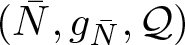
Since the Killing field X, present on any quaternionic Kähler manifold  $(\bar N,g_{\bar N},\mathcal{Q})$ in the image of the HK/QK correspondence, has nowhere-vanishing quaternionic moment map [Reference Dyckmanns15],
 $\bar N$ always carries an integrable almost complex structure [Reference Salamon28, § 7]. This complex structure, which we call J 1, is compatible with the quaternionic structure
 $\mathcal{Q}$. Changing the sign of J 1 on the two-dimensional (2D) distribution spanned by X and
 $J_1 X$ yields another natural almost complex structure, which we call
 $\tilde J_1$. Note that
 $\tilde J_1$ is never compatible with
 $\mathcal{Q}$ since it induces the opposite orientation.
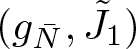
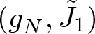
In this article, we study the properties of the almost Hermitian structure  $(\tilde J_1,g_{\bar N})$. In particular, we are interested to know when
 $\tilde J_1$ is also integrable, in which case we refer to the quaternionic Kähler manifold as a doubly integrable HK/QK manifold. Accordingly, our first main result, theorem 3.2, is a necessary and sufficient condition for the integrability of
 $\tilde J_1$:
Theorem 1.
Let  $(\bar N,g_{\bar N},\mathcal{Q})$ be a (pseudo-)quaternionic Kähler manifold that arises from the HK/QK correspondence applied to a pseudo-hyper-Kähler manifold
 $(N,g_N,I_1,I_2,I_3)$ endowed with rotating Killing field Z. Then the almost complex structure
 $\tilde J_1$ on
 $\bar N$ is integrable if and only if there exists a smooth function ψ on the dual pseudo-hyper-Kähler manifold N such that the identity
 $\nabla_Z Z=\psi I_1 Z$ holds.
In the case where  $\bar N$ arises from the c-map, the equation
 $\nabla_Z Z=\psi I_1 Z$ is satisfied with
 $\psi\equiv -1$ (see [Reference Alekseevsky, Cortés and Mohaupt4, Prop. 2]) and therefore the class of doubly integrable HK/QK manifolds includes the (one-loop deformed) c-map spaces. This extends earlier results from [Reference Cortés, Dempster, Mohaupt and Vaughan8].
Given a doubly integrable HK/QK manifold, one may inquire as to further properties of the Hermitian structure  $(\tilde J_1,g_{\bar N})$. On the one hand, it is known that no quaternionic Kähler manifold, with exception of manifolds locally isometric to the Grassmannian of complex two planes or to its non-compact dual, is Kähler. On the other hand, based on the study of Einstein metrics conformal to Kähler metrics, see [Reference Derdzinski and Maschler14] and references therein, one may suspect that, at least in some cases, the quaternionic Kähler metric could be conformal to a Kähler metric. We prove that this is indeed the case in dimension 4 (cf. theorem 5.6), but never so in higher dimensions (cf. theorem 5.7):
Theorem 2.
Let  $(\bar N,g_{\bar N},\mathcal{Q})$ be a doubly integrable HK/QK manifold. Then
 $g_{\bar N}$ is conformal to a Kähler metric compatible with the complex structure
 $\tilde J_1$ and invariant under the canonical Killing field X if and only if
 $\bar N$ is a fourfold.
While (deformed) c-map spaces are doubly integrable HK/QK manifolds, with  $(\tilde J_1,g_{\bar N})$ moreover being conformally Kähler in dimension 4 by virtue of the above result, they do not exhaust the class of doubly integrable HK/QK manifolds. To prove this, we show in theorem 6.1 that every fourfold in this class is locally isometric to a member of a three-dimensional (3D) family
 $g^{a,b,c}$ of metrics. Since there is only a single c-map space in dimension 4 (carrying a one-parameter family of metrics), this gives us non-trivial examples beyond the c-map, which we analyse in some detail. In particular, we prove that they are either locally symmetric or are of cohomogeneity 1. In the latter case, we give an explicit action generated by a Lie algebra of Killing fields isomorphic to either
 $\mathfrak{o}(2) \lt imes\mathfrak{heis}_3(\mathbb R)$,
 $\mathfrak{u}(2)$, or
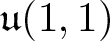
 $\mathfrak{u}(1,1)$ (cf. proposition 6.4).
The article is organized as follows. We recall some preliminaries regarding the HK/QK correspondence and c-map in §2, after which we prove theorem 1 in §3. In §4, we study a distinguished family of examples  $(\bar N_n,g^c_n)$,
 $n\in \mathbb{N}$,
 $c\geq 0$, for which we have a third integrable almost complex structure. The metrics
 $g^c_n$ are a one-parameter deformation of the non-compact symmetric space
 $\frac{\mathrm{SU}(n,2)}{\mathrm{S}(\mathrm U(n)\times \mathrm U(2))}$ (which corresponds to c = 0) through complete quaternionic Kähler metrics. They have been extensively studied, see, e.g., [Reference Cortés, Röser and Thung11, Reference Cortés, Saha and Thung13]. We take up the question of finding a Kähler metric in the same conformal class as the quaternionic Kähler metric in §5, proving theorem 2. Finally, §6 is dedicated to an in-depth analysis of the four-dimensional (4D) case, for which we give a local classification. We conclude with a detailed examination of the local models.
2. Quaternionic Kähler manifolds from the HK/QK correspondence
In this preparatory section, we recall the HK/QK correspondence in some detail as well as the properties of the resulting quaternionic Kähler manifolds that we will need later on. For more details, see [Reference Alekseevsky, Cortés, Dyckmanns and Mohaupt3, Reference Cortés, Saha and Thung12, Reference Macia and Swann25] and references therein.
2.1. Twists and the HK/QK correspondence
The starting point for the HK/QK correspondence is a pseudo-hyper-Kähler manifold  $(N,g_N,I_k)$,
 $k=1,2,3$, endowed with a distinguished vector field.
Definition 2.1. A vector field Z on a pseudo-hyper-Kähler manifold  $(N,g_N,I_k)$ such that
 $g_N(Z,Z)$ is nowhere-vanishing is called a rotating Killing field if it satisfies
 $L_Zg_N=0$,
 $L_ZI_1=0$, and
 $L_ZI_2=I_3$.
In order to apply the HK/QK correspondence, we ask that  $(N,g_N,I_k)$ comes equipped with a rotating Killing field Z which is Hamiltonian with respect to the two-form
 $\omega_\mathrm{H}=\omega_1+\mathrm{d}(g_N(Z,-))$, where ω 1 is the Kähler form associated with I 1. Furthermore, we will require that the Hamiltonian function, which we denote by
 $f_\mathrm{H}$, is nowhere-vanishing. We remark that, under these assumptions, Z is automatically Hamiltonian with respect to ω 1, with Hamiltonian function
 $f_Z:= f_\mathrm{H}-g_N(Z,Z)$. We will also assume that fZ is nowhere-vanishing.
Under the assumption that ω 1 is an integral form, the triple  $(Z,\omega_\mathrm{H},f_\mathrm{H})$ forms twist data on N in the sense of A. Swann [Reference Swann29]. In particular, there exists a principal circle bundle
 $\pi_N\colon P\to N$ with connection η whose curvature is
 $\omega_\mathrm{H}$, and Z lifts to a vector field ZP on P that preserves η. Explicitly, we have
 \begin{equation}
Z_P=\tilde Z+\pi_N^*f_\mathrm{H} X_P
\end{equation}
where XP generates the principal circle action on P and  $\tilde Z$ is the η-horizontal lift of Z. The quotient space
 $\bar N:= P/\langle Z_P\rangle$ is then called the twist of N with respect to the twist data
 $(Z,\omega_\mathrm{H},f_\mathrm{H})$. Under the assumption that Z and ZP act freely and properly, it is a smooth manifold. Note that
 $\bar N$ comes equipped with a distinguished vector field X, obtained by pushing down XP.
The power of the twist construction lies in the fact that Z-invariant structures on N can be carried over to  $\bar N$. For instance, if φ is an invariant function on N, then
 $\pi^*_N\varphi\in C^\infty(P)$ is invariant under ZP and therefore induces a well-defined function ψ on
 $\bar N$, which we will call the twist of φ. Similarly, we can push down the η-horizontal lift
 $\tilde U$ of an invariant vector field U on N to obtain its twist
 $V=d \pi_{\bar N}(\tilde U)$ on
 $\bar N$. Twists of arbitrary tensor fields are then defined by demanding compatibility of twisting with tensor products and contractions. By comparing lifts to P, one can work out explicit formulas for the twist of a tensor field without much effort.
The following Lemmata, whose proofs can be found in [Reference Swann29], follow from such computations:
Lemma 2.2. If α is an invariant p-form on N and β denotes its twist with respect to the twist data  $(Z,\omega_\mathrm{H},f_\mathrm{H})$, then
 $\mathrm{d} \beta$ is the twist of
 $\mathrm{d} \alpha-f_\mathrm{H}^{-1}\omega_\mathrm{H}\wedge\iota_Z\alpha$.
Lemma 2.3. The twist of an invariant complex structure I on N with respect to the twist data  $(Z,\omega_\mathrm{H},f_\mathrm{H})$ is integrable if and only if
 $\omega_\mathrm{H}$ is of type
 $(1,1)$ with respect to I.
Returning to the setting of the HK/QK correspondence, let  $(N,g_N,I_k,Z)$,
 $k=1,2,3$, be a pseudo-hyper-Kähler manifold endowed with a rotating Killing field Z, and consider the twist data
 $(Z,\omega_\mathrm{H},f_\mathrm{H})$ as above.
Proposition 2.4. [Reference Cortés, Saha and Thung13, § 2.3]
Let  $\nabla$ denote the Levi-Civita connection of
 $(N,g_N)$. Then the endomorphism field
 $I_\mathrm{H}=I_1+2\nabla Z$ satisfies the relation
 $g_N(I_\mathrm{H}-,-)=\omega_\mathrm{H}$, is skew-symmetric with respect to gN, and commutes with each Ik. In particular, the two-form
 $\omega_\mathrm{H}$ is of type
 $(1,1)$ with respect to each Ik.
The quaternionic structure bundle  $\langle I_1,I_2,I_3\rangle\subset \operatorname{End}(TN)$ is invariant under Z and therefore induces an almost quaternionic structure
 $\mathcal{Q}$ on the resulting twist manifold
 $\bar N$ (with respect to the twist data
 $(Z,\omega_\mathrm{H},f_\mathrm{H})$ as above). In fact, it is known [Reference Alekseevsky, Cortés, Dyckmanns and Mohaupt3, Reference Macia and Swann25] that
 $(\bar N,\mathcal{Q})$ carries a compatible quaternionic Kähler metric
 $g_{\bar N}$. This metric, however, is not the twist of the pseudo-hyper-Kähler metric gN, but rather of its so-called elementary deformation
 $g_\mathrm{H}$ [Reference Macia and Swann25]. The elementary deformation
 $g_\mathrm{H}$ is related to gN by the formula
 \begin{equation}
g_\mathrm{H}= \frac{1}{f_Z}g_N|_{(\mathbb{H} Z)^\perp}+\frac{f_\mathrm{H}}{f_Z^2}g_N|_{\mathbb{H} Z}
\end{equation}
where  $\mathbb{H} Z=\langle Z,I_1 Z,I_2Z,I_3Z\rangle$ denotes the quaternionic span of Z. We say that the quaternionic Kähler manifold
 $(\bar N,g_{\bar N},\mathcal{Q})$ arises from the HK/QK correspondence applied to N. Since the signature of a metric is preserved by twisting, the quaternionic Kähler metric
 $g_{\bar N}$ is positive definite if and only if
 $g_\mathrm{H}$ is. From (2), we see that this may happen even if gN has signature
 $(4k,4)$, as long as
 $f_Z \gt 0$ and
 $f_\mathrm{H} \lt 0$. This observation is crucial in applying the HK/QK correspondence to the c-map [Reference Alekseevsky, Cortés and Mohaupt4]. Since we are interested primarily in positive-definite quaternionic Kähler metrics, we will from now on assume that
 $g_\mathrm{H}$ is Riemannian (though our results remain valid, mutatis mutandis, in the indefinite case).
Note that the above construction depends on our choice of Hamiltonian function  $f_\mathrm{H}$, which appears explicitly in the expression for the elementary deformation
 $g_\mathrm{H}$, whose twist is the quaternionic Kähler metric
 $g_{\bar N}$. Since there is always a one-parameter freedom in choosing a Hamiltonian function, the HK/QK correspondence in fact yields a one-parameter family of quaternionic Kähler metrics on
 $\bar N$.
We note the following property of quaternionic Kähler manifolds resulting from the HK/QK correspondence:
Proposition 2.5. Every quaternionic Kähler manifold that arises from the HK/QK correspondence admits an integrable complex structure compatible with the metric and quaternionic structure.
Proof. This follows immediately from applying lemma 2.3 to the invariant complex structure I 1 on the hyper-Kähler manifold, using proposition 2.4, and noting that I 1 is compatible with the elementary deformation and quaternionic structure on the hyper-Kähler side of the correspondence.
2.2. The c-map
In order to put the HK/QK correspondence to use, we need a way to construct pseudo-hyper-Kähler manifolds endowed with a rotating Killing field. The theory of special Kähler manifolds provides a plentiful source of examples.
Definition 2.6. An affine special Kähler manifold is a pseudo-Kähler manifold  $(M,g_M,J_M)$ endowed with a flat, torsion-free and symplectic connection
 $\nabla^{\mathrm{SK}}$ such that
 $\nabla^{\mathrm{SK}} J_M$ is symmetric. An affine special Kähler manifold is called conical (or a CASK manifold) if it admits a vector field ξ such that
 $\nabla^{\mathrm{SK}} \xi=\nabla^{g_M}\xi=\operatorname{id}_{TM}$, where
 $\nabla^{g_M}$ denotes the Levi-Civita connection of gM. Moreover, we require that
 $\{\xi,J_M\xi\}$ generate a principal
 $\mathbb{C}^*$-action, and that
 $g_M(\xi,\xi) \lt 0$ while gM is positive-definite on
 $\langle \xi,J_M\xi\rangle^\perp$.
We recall how to construct a pseudo-hyper-Kähler manifold N with rotating Killing field from a CASK manifold  $(M,g_M,J_M,\nabla^{\mathrm{SK}},\xi)$ of real dimension
 $2n+2$. The smooth manifold underlying N is
 $T^*M$. Now note that the special Kähler connection
 $\nabla^{\mathrm{SK}}$ induces a splitting
 $T(T^*M)\cong \pi^*T^*M\oplus \pi^*TM$. With respect to this splitting, we define the tensor fields
 \begin{equation}
g_N=
\begin{pmatrix}
g_M & 0 \\ 0 & g^{-1}_M
\end{pmatrix}
\qquad
I_1=
\begin{pmatrix}
J_M & 0 \\ 0 & J_M^*
\end{pmatrix}
\qquad
I_2=
\begin{pmatrix}
0 & -\omega_M^{-1} \\ \omega_M & 0
\end{pmatrix}
\qquad
I_3=I_1I_2
\end{equation}
where we have omitted pullbacks throughout to simplify notation. It is well-known (see, e.g., [Reference Alekseevsky, Cortés and Devchand2] and references therein) that these tensor fields define a pseudo-hyper-Kähler structure on  $N=T^*M$ of quaternionic signature
 $(n,1)$. This construction is known as the rigid c-map. Moreover, the
 $\nabla^{\mathrm{SK}}$-horizontal lift of
 $-J_M\xi$ to N endows it with a canonical rotating Killing field Z [Reference Alekseevsky, Cortés and Mohaupt4].
This construction gives rise to many examples, since there is an abundance of CASK manifolds. Indeed, if  $U\subset \mathbb{C}^n$ is any
 $\mathbb{C}^*$-invariant domain, there is a CASK manifold associated with any generic holomorphic function on U which is homogeneous of degree 2 under the
 $\mathbb{C}^*$-action, see [Reference Alekseevsky, Cortés and Devchand2] for more detailed statements.
It follows easily from the definitions that the vector field  $-J_M\xi$ on a CASK manifold M is Killing and Hamiltonian with negative Hamiltonian function
 $\frac{1}{2}g_M(\xi,\xi)$, so we may consider the Kähler quotient
 $M\ \unicode{x2AFD}\ S^1=\mu^{-1}\big(-\frac{1}{2}\big)/S^1$ with respect to the circle action it generates.
Definition 2.7. Let  $(M,g_M,J_M,\nabla^{\mathrm{SK}},\xi)$ be a CASK manifold. Then the Kähler quotient
 $\bar M =M\ \unicode{x2AFD}\ S^1$ with respect to the Hamiltonian circle action generated by
 $-J_M\xi$ is called a PSK manifold.
Note that the induced Kähler metric on a PSK manifold is always positive-definite.
By this (extrinsic) definition, giving a PSK structure on a manifold is equivalent to giving the corresponding CASK manifold, and the two manifolds can be used interchangeably for our purposes. Thus, we may say that, starting from a PSK manifold, we may pass to the associated CASK manifold and apply the rigid c-map construction and the HK/QK correspondence to obtain a quaternionic Kähler manifold. Thus, we have obtained a method to associate quaternionic Kähler manifolds to PSK manifolds (cf. [Reference Alekseevsky, Cortés, Dyckmanns and Mohaupt3]). This construction recovers what is known as the (supergravity) c-map [Reference Ferrara and Sabharwal16].
Recall that we obtain not just one, but an entire one-parameter family of quaternionic Kähler metrics from a single hyper-Kähler manifold with rotating Killing vector field by varying the corresponding Hamiltonian function. In the case of the c-map, there is a distinguished choice of Hamiltonian. We call the corresponding quaternionic Kähler metric the undeformed c-map metric and denote it by  $g_{\bar N}^0$. The quaternionic Kähler metrics that arise from different choices of Hamiltonian function obtained by shifting the distinguished one by a constant
 $c\in \mathbb{R}$ are known as (one-loop) deformed c-map metrics [Reference Llana, Saueressig and Vandoren24] and denoted by
 $g_{\bar N}^c$. It turns out that these metrics have good completeness properties only if we restrict to
 $c\geq 0$ [Reference Cortés, Dyckmanns and Suhr9], which we will do from now on.
3. A Hermitian structure inducing the opposite orientation
Let  $(\bar{N},g_{\bar{N}},\mathcal{Q})$ be a quaternionic Kähler manifold obtained by the HK/QK correspondence from a pseudo-hyper-Kähler manifold
 $(N,g_N,I_1,I_2,I_3)$ endowed with rotating Killing field Z, as described in §2. Recall that it inherits a distinguished vector field X from the generator of the principal circle action on
 $\pi_N\colon P\to N$. This vector field, which we can also view as the twist of the vector field
 $-f_\mathrm{H}^{-1}Z$ on N (cf. Eq. (1)), is Killing with respect to
 $g_{\bar N}$. Its quaternionic moment map µ X is nowhere-vanishing and therefore defines an integrable complex structure
 \begin{equation}
J_1 := -\frac{\mu^X}{\| \mu^X\|} \in \Gamma (\mathcal{Q}),
\end{equation}
see [Reference Dyckmanns15, Rem. 4.1.6]. This is, in fact, just another way of describing the complex structure whose existence is guaranteed by proposition 2.5. We shall refer to the vector field X as the canonical Killing field on  $\bar N$.
Now let  $\mathcal{D}$ be the rank-2 distribution spanned by X and
 $J_1X$. We define a new skew-symmetric almost complex structure
 $\tilde{J}_1$ by
 \begin{equation*}
\tilde{J}_1|_\mathcal{D} := -J_1|_\mathcal{D},\quad
\tilde{J}_1|_{\mathcal{D}^\perp} := J_1|_{\mathcal{D}^\perp}.
\end{equation*}
The orientation defined by  $\tilde{J}_1$ is opposite to the one defined by
 $\mathcal{Q}$.
Definition 3.1. A quaternionic Kähler manifold  $(\bar{N},g_{\bar{N}},\mathcal{Q})$ obtained by the HK/QK correspondence is said to be a doubly integrable HK/QK manifold if the almost complex structure
 $\tilde{J}_1$ defined above is integrable.
Theorem 3.2. Let  $\bar{N}$ be obtained from N by the HK/QK correspondence as summarized above. Then it is a doubly integrable HK/QK manifold if and only if the vector field
 $\nabla_Z Z$ on N is a section of the vector bundle
 $\langle Z,I_1 Z\rangle$. In this case, we have a Hermitian structure
 $(g_{\bar{N}},\tilde{J}_1)$ compatible with the opposite orientation.
Since Z is Killing and  $g_N(Z,Z)$ is nowhere-vanishing, the above condition is equivalent to requiring that
 $\nabla_Z Z=\psi I_1 Z$ for some smooth function ψ on N. Contracting with gN and again using that Z is Killing, this becomes
 $\frac{1}{2}\mathrm{d} (g_N(Z,Z)) = -\psi\, \mathrm{d} f_Z$.
It is known that this holds when the pseudo-hyper-Kähler manifold N with rotating Killing field Z arises by applying the rigid c-map to a CASK manifold M. Indeed, in [Reference Alekseevsky, Cortés and Mohaupt4, Prop. 2], it is shown that, in this case, the identity  $\nabla_Z Z=-I_1 Z$ holds (with our conventions). Let
 $\bar M$ denote the PSK manifold associated with M. Then the corresponding one-parameter family of quaternionic Kähler manifolds
 $(\bar N,g_{\bar N}^c)$ arise from the (deformed) c-map applied to
 $\bar M$. Therefore, the following result is a corollary of the previous theorem.
Theorem 3.3. Any quaternionic Kähler manifold  $(\bar{N},g_{\bar{N}})$ obtained from the (deformed) c-map construction admits a Hermitian structure
 $(g_{\bar{N}},\tilde{J}_1)$ compatible with the opposite orientation.
In order to prove theorem 3.2, we will need a lemma.
Lemma 3.4. The condition  $\nabla_Z Z\in \Gamma(\langle Z,I_1 Z\rangle)$ is equivalent to
 $\mathrm{d}(g_{\bar{N}}(X,X))|_{(J_1X)^\perp} =0$.
Proof. Since  $g_N(\nabla_Z Z,Z)=0$ by the Killing equation, the condition
 $\nabla_Z Z\in\Gamma(\langle Z,I_1 Z\rangle)$ is equivalent to
 $\mathrm{d}(g_N(Z,Z))|_{(I_1Z)^\perp} =0$. To see that the latter is, in turn, equivalent to
 $\mathrm{d}(g_{\bar{N}}(X,X))|_{(J_1X)^\perp}=0$ it suffices to go through the HK/QK correspondence.
It follows from (1) that X is the twist of the vector field  $-f_\mathrm{H}^{-1}Z$ on N. Since
 $g_{\bar N}$ is the twist of
 $g_\mathrm{H}$, it follows that the function
 $g_{\bar{N}}(X,X)$ is the twist of
 $\frac{1}{f_\mathrm{H}^2}g_\mathrm{H}(Z,Z)$. Recall that
 $g_\mathrm{H}$ differs from gN by a rescaling on
 $\mathbb{H} Z$ and on
 $(\mathbb{H} Z)^\perp$, with factors involving only the Z-invariant functions fZ and
 $f_\mathrm{H}$ (cf. Eq. (2)). Since
 $\mathrm{d} f_Z=-\iota_Z\omega_1$ and
 $\mathrm{d} (g_N(Z,Z))$ vanish on
 $(I_1Z)^\perp$, the same holds for
 $\mathrm{d}\big(\frac{1}{f_\mathrm{H}^2}g_\mathrm{H}(Z,Z)\big)$. Now, the fact that the complex structure J 1 is the twist of I 1 implies that the twist
 $g_{\bar{N}}(X,X)$ of the function
 $\frac{1}{f_\mathrm{H}^2} g_\mathrm{H}(Z,Z)$ satisfies
 $\mathrm{d} (g_{\bar{N}}(X,X))|_{(J_1X)^\perp}=0$ as well.
Proof. Proof of theorem 3.2
We denote by  $\mathcal{D}^{1,0}$ and
 $(\mathcal{D}^\perp)^{1,0}$ the i-eigenbundles of
 $\tilde{J}_1$ on
 $\mathcal{D}_{\mathbb{C}}$ and
 $\mathcal{D}^\perp_{\mathbb{C}}$, respectively.
 $\mathcal{D}^{0,1}$ and
 $(\mathcal{D}^\perp)^{0,1}$ signify the corresponding −i-eigenbundles. The distribution
 $\mathcal{D}^{1,0}= \langle X+iJ_1X\rangle$ is involutive for dimensional reasons. We first prove that
 $(\mathcal{D}^\perp)^{1,0}$ is also involutive.
Let  $Y, Z\in \Gamma(\mathcal{D}^\perp)$. Then
 $[Y-iJ_1Y,Z-iJ_1Z]$ is of type
 $(1,0)$ with respect to J 1 by integrability of J 1. To prove that it is also of type
 $(1,0)$ with respect to
 $\tilde{J}_1$ it suffices to check that its projection onto
 $\mathcal{D}^{0,1}$ vanishes, which in turn follows from
 \begin{equation*}
g_{\bar{N}}(X+iJ_1X,[Y-iJ_1Y,Z-iJ_1Z])=0
\end{equation*}
or, equivalently,
 \begin{equation*}
[Y,Z]-[J_1Y,J_1Z] -J_1([J_1Y,Z]+[Y,J_1Z]) \perp \mathcal{D}.
\end{equation*}
Defining the one-forms  $\alpha=g_{\bar N}(X,-)$ and
 $\beta=g_{\bar N}(J_1 X,-)$, this amounts to showing that
 $\mathrm{d}\alpha|_{{\bigwedge}^2 \mathcal{D}}$ and
 $\mathrm{d}\beta|_{{\bigwedge}^2 \mathcal{D}}$ are of type
 $(1,1)$ with respect to J 1. For α, this follows by combining the fact that µ X is proportional to
 $(\nabla X)^{\mathfrak{sp}_1}$ and the definition of J 1 (see (4)) to deduce that
 $\nabla X$ commutes with J 1. To show it for β, we remark that the vanishing of the Nijenhuis tensor of J 1 implies
 \begin{equation*}
J_1([X,Y]-[J_1X,J_1Y]) = [X,J_1Y]+[J_1X,Y].
\end{equation*}
Therefore
 \begin{equation*}
\beta ([Y,Z]-[J_1Y,J_1Z]) = -\alpha ([Y,J_1Z]+[J_1Y,Z]).
\end{equation*}
So the claimed property for β follows from that for α.
To establish the integrability of  $\tilde J_1$ it now suffices to prove that
 $X+iJ_1X$ preserves
 $(\mathcal{D}^\perp)^{1,0}$. Note that X and
 $J_1X$ are real holomorphic vector fields with respect to both J 1 and
 $\tilde{J}_1$. In addition, X is Killing and therefore preserves not only
 $\mathcal{D}$ but also
 $\mathcal{D}^\perp$. As a consequence, X preserves the complex distribution
 $(\mathcal{D}^\perp)^{1,0}$. To show that this distribution is also
 $J_1X$-invariant it suffices to show that
 $J_1X$ preserves
 $\mathcal{D}^\perp$. This means that we have to verify that
 $\alpha([J_1X,Y])=\beta([J_1 X,Y])=0$ for all
 $Y\perp \mathcal{D}$. Using that
 $J_1X$ is J 1-holomorphic, one can easily see that the second condition actually follows from the first.
Decomposing  $\nabla X$ into its part
 $(\nabla X)^{\mathfrak{sp}_1}=\mu^X$ in
 $\mathcal{Q}$, which is proportional to J 1, and the part
 $(\nabla X)^{\mathfrak{sp}_n}$ (n being the quaternionic dimension of
 $\bar N$) in the centralizer of
 $\mathcal{Q}$ we see that (for all
 $Y\perp \mathcal{D}$)
 \begin{equation*}
\alpha ([J_1X,Y])= -\mathrm{d}\alpha (J_1X,Y)= -2g_{\bar{N}}((\nabla X)^{\mathfrak{sp}_n}J_1X,Y)
=2g_{\bar{N}}((\nabla X)^{\mathfrak{sp}_n}X,J_1Y).
\end{equation*}
Thus,  $\tilde J_1$ is integrable if and only if
 $(\nabla X)^{\mathfrak{sp}_n}X$ is a section of
 $\mathcal{D}$ or, equivalently, if
 $\nabla_XX$ is. Since
 $Xg_{\bar{N}}(X,X)=0$, the latter is equivalent to
 $\mathrm{d}(g_{\bar{N}}(X,X))|_{(J_1X)^\perp} =0$, which, in turn, is equivalent to the condition
 $\nabla_Z Z\in \Gamma(\langle Z,I_1 Z\rangle)$, by lemma 3.4.
It was already known that  $\tilde J_1$ is integrable if the quaternionic Kähler manifold
 $(\bar N,g_{\bar N})$ arises from the undeformed c-map [Reference Cortés, Dempster, Mohaupt and Vaughan8, Thm. 1 (a)], so we may think of theorem 3.3 as an extension of this result to the one-loop deformed c-map. Theorem 3.2 and its proof put it in the natural, broader context of the HK/QK correspondence.
There are a number of reformulations of the integrability condition, some of which will be of use later on:
Lemma 3.5. The following conditions are equivalent:
(a)
 $\nabla_Z Z$ is a section of the rank-2 distribution $\langle Z,I_1 Z\rangle$.
(b)
$\mathrm{d} (g_N(Z,Z))\wedge \mathrm{d} f_Z=0$.(c)
$\mathrm{d} f_\mathrm{H}\wedge \mathrm{d} f_Z=0$.(d) There exists a smooth function ψ such that one of the following equivalent identities holds:
(i)
$\nabla_Z Z=\psi I_1Z$.(ii)
$I_\mathrm{H} Z=(1+2\psi) I_1 Z$.(iii)
$\mathrm{d} (g_N(Z,Z))=2\psi \mathrm{d} f_Z$.(iv)
$\mathrm{d} f_\mathrm{H}=(1+2\psi)\mathrm{d} f_Z$.


Proof. First, let us check the equivalence of the conditions listed in (d). That (i) and (ii) are equivalent follows from  $I_\mathrm{H}=I_1+2\nabla Z$. For an arbitrary vector field Y, the following identity holds:
 \begin{equation*}
g_N(\nabla_Z Z,Y)=-g_N(\nabla_Y Z,Z)=-\tfrac{1}{2}\mathrm{d} (g_N(Z,Z))(Y).
\end{equation*}
Now (i) holds if and only if  $g_N(\nabla_Z Z,Y)=-\psi\,\mathrm{d} f_Z(Y)$, which is to say
 $\mathrm{d} (g_N(Z,Z))=2\psi\,\mathrm{d} f_Z$, i.e., condition (iii) holds. Moreover, (iii)
 $\Longleftrightarrow$ (iv) since
 $f_\mathrm{H}=f_Z+g_N(Z,Z)$.
It is obvious that (b) and (c) are equivalent to (d), (iii) and (d), (iv), respectively. Finally, the equivalence of (a) and (d), (i) follows directly from the Killing equation.
4. Examples carrying a third Hermitian structure
Among the simplest examples of PSK manifolds are the complex hyperbolic spaces  $\mathbb{C} H^n$. The corresponding CASK manifolds are
 \begin{equation*}
M_{n+1}:= \bigg\{(z_0,\dots,z_n)\in \mathbb{C}^{n+1}\bigg|\, \lvert z_0 \rvert^2 \gt \sum_{j=1}^n \lvert z_j \rvert^2\bigg\}
\end{equation*}
equipped with the flat Kähler structure defined by the Hermitian form
 \begin{equation*}
h=-\mathrm{d} z_0\otimes \mathrm{d} \bar z_0+\sum_{j=1}^n \mathrm{d} z_j\otimes\mathrm{d} \bar z_j.
\end{equation*}
The conical structure is induced by the standard  $\mathbb{C}^*$-action by complex multiplication. In particular, we have
 \begin{equation*}
-J\xi =-i \sum_{j=0}^n \bigg(z_j \frac{\partial }{\partial z_j}-\bar z_j \frac{\partial }{\partial \bar z_j}\bigg).
\end{equation*}
Applying the c-map to  $\mathbb{C} H^n$, we obtain a one-parameter family of complete quaternionic Kähler manifolds
 $(\bar N_{n+1},g_{n+1}^c)$,
 $c\geq 0$, of dimension
 $4n+4$. The undeformed c-map metric yields a quaternionic Kähler symmetric space, while the deformed c-map metrics are of cohomogeneity 1 [Reference Cortés, Saha and Thung12, Reference Cortés, Saha and Thung13]. We denote the corresponding hyper-Kähler manifold by
 $N_{n+1}$.
Proposition 4.1. The endomorphism field  $I_\mathrm{H}$ (defined in proposition 2.4) on Nn is an integrable almost complex structure inducing the same orientation as
 $\mathcal{Q}$ if n is even and the opposite orientation if n is odd.
Proof. Observe that  $N_n\cong M_n\times \mathbb{C}^n$ is nothing but an open subset of a quaternionic vector space, endowed with the standard hyper-Kähler structure of quaternionic signature
 $(n-1,1)$. In particular, Nn is a product of complex manifolds and I 1 is the induced complex structure corresponding to this product structure. Using coordinates
 $(z_0,\dots,z_{n-1},w_0,\dots,w_{n-1})$ adapted to the product structure, we see that the rotating Killing field on Nn is given by
 \begin{equation*}
Z=-i \sum_{j=0}^{n-1} \bigg(z_j\frac{\partial }{\partial z_j}-\bar z_j \frac{\partial }{\partial \bar z_h}\bigg).
\end{equation*}
Decomposing  $TN_n\cong TM_n\oplus T\mathbb{C}^n$, one now easily sees that
 \begin{equation*}
\nabla Z=
\begin{pmatrix}
-I_1|_{TM_n} & 0 \\ 0 & 0
\end{pmatrix}
\end{equation*}
and correspondingly
 \begin{equation*}
I_\mathrm{H} = I_1+2\nabla Z=
\begin{pmatrix}
- I_1|_{TM_n} & 0 \\ 0 & I_1|_{T\mathbb{C}^n}
\end{pmatrix}.
\end{equation*}
In summary,  $I_\mathrm{H}$ the natural induced complex structure on the product
 $\overline{M_n}\times \mathbb{C}^n$ of complex manifolds, where
 $\overline{M_n}$ denotes the conjugate of the complex manifold Mn. In particular,
 $I_\mathrm{H}$ is integrable.
The claim regarding the orientation follows immediately from the fact that  $TM_n\subset TN_n$ is a distribution of real dimension 2n.
Theorem 4.2. For any  $n\geq 2$, the quaternionic Kähler manifolds
 $(\bar N_n,g_n^c)$,
 $c\geq 0$, that arise from the c-map applied to
 $\mathbb{C} H^{n-1}$ admit a third complex structure
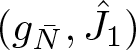
 $\hat J$. The associated Hermitian structure
 $(g_n^c,\hat J)$ induces the same orientation as
 $\mathcal{Q}$ if and only if n is even.
Proof. It should not be surprising that we define  $\hat J$ as the twist of the integrable complex structure
 $I_\mathrm{H}$. Since
 $I_\mathrm{H}$ is skew with respect to
 $g_{N_n}$ by proposition 2.4, the twisting two-form
 $\omega_\mathrm{H}$ is of type
 $(1,1)$ with respect to
 $I_\mathrm{H}$. By lemma 2.3,
 $\hat J$ is then integrable. Furthermore,
 $I_\mathrm{H}$ is compatible with
 $g_\mathrm{H}$, so
 $\hat J$ is compatible with its twist
 $g_n^c$. The claim regarding the induced orientation follows immediately from the corresponding statement for
 $I_\mathrm{H}$, since twisting preserves algebraic properties.
Remark 4.3. In the case n = 1, where one applies the c-map to a single point, the complex structures  $\hat J$ and
 $\tilde J_1$ coincide. In higher dimensions they do not, since
 $\hat J$ differs from J 1 by a sign on a half-dimensional distribution while
 $\tilde J_1$ differs from J 1 on a 2D distribution.
Again, in the case of the undeformed c-map, the existence of the Hermitian structure defined by  $\hat J$ had already been established in [Reference Cortés, Dempster, Mohaupt and Vaughan8, Thm. 2 (a)]. Theorem 4.2 generalizes it to the deformed c-map and provides an interpretation in terms of the HK/QK correspondence.
5. The conformal Kähler property
Proposition 5.1. The members of the one-parameter family  $g_1^c$,
 $c\geq 0$, of quaternionic Kähler metrics on the self-dual Einstein four-manifold
 $\bar N_1$ are all conformal to a Kähler metric compatible with the complex structure
 $\tilde J_1$. In other words, the Hermitian structures
 $(g_1^c,\tilde J_1)$,
 $c\geq 0$, are conformally Kähler.
Proof. We start by considering the hyper-Kähler manifold N 1. Because we are in the 4D case, we have  $TN_1=\mathbb{H} Z$, so that in particular the elementary deformation consists only of a conformal rescaling:
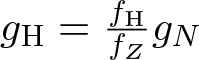 $g_\mathrm{H}=\frac{f_\mathrm{H}}{f_Z}g_N$. Correspondingly, the quaternionic Kähler metric
 $g_1^c$, with
 $c\geq 0$ arbitrary, is a conformal rescaling of the twist of
 $g_{N_1}$, which we will denote by hc.
Recall that a Hermitian structure is conformally Kähler if and only if the associated fundamental two-form σ satisfies  $\mathrm{d} \sigma=\theta\wedge\sigma$ for an exact one-form θ. We will now show that this is the case for the structure
 $(h^c,\tilde J_1)$. It follows from remark 4.3 that
 $\tilde J_1$ is the twist of
 $I_\mathrm{H}$, which satisfies
 $g_{N_1}(I_\mathrm{H}-,-)=\omega_\mathrm{H}$. This shows that the fundamental two-form σ associated with the Hermitian structure
 $(h^c,\tilde J_1)$ is nothing but the twist of
 $\omega_\mathrm{H}$.
We now use lemma 2.2 and conclude that the exterior derivative of σ is the twist of the form
 \begin{equation*}
\mathrm{d} \omega_\mathrm{H}-\frac{1}{f_\mathrm{H}}\iota_Z\omega_\mathrm{H} \wedge \omega_\mathrm{H}
=\mathrm{d}(\log f_\mathrm{H})\wedge\omega_\mathrm{H}.
\end{equation*}
Now write ψ for the twist of the Z-invariant function  $\log f_\mathrm{H}$. Then, again by lemma 2.2,
 $\mathrm{d} \psi$ is the twist of
 $\mathrm{d} \log f_\mathrm{H}$ and we conclude that
 \begin{equation*}
\mathrm{d}\sigma=\mathrm{d}\psi\wedge\sigma.
\end{equation*}
Since hc and g c1 are conformally equivalent, this proves that the Hermitian structure  $(g^c_1,\tilde J_1)$ is conformally Kähler.
Remark 5.2. In dimensions 4n,  $n\geq 2$, the hyper-Kähler metric
 $g_{N_n}$ is indefinite of signature
 $(4n-4,4)$ and therefore so is its twist hc. The above proof still shows that hc is conformal to a pseudo-Kähler metric, but we can no longer use this to draw the same conclusion about
 $g_n^c$ since the relationship between
 $g_{N_n}$ and
 $g_\mathrm{H}$ is more complicated for n > 1 (cf. Eq. (2)).
The quaternionic Kähler four-manifolds  $(\bar N_1,g^c_1)$,
 $c\geq 0$, are examples of half conformally flat Einstein four-manifolds that admit a principal isometric action of a 3D Heisenberg group. These have recently been classified in arbitrary signature [Reference Cortés and Murcia10]. It turns out that such manifolds are always conformally Kähler or conformally para-Kähler, in accordance with proposition 5.1.
In light of the above, it is natural to ask whether every doubly integrable HK/QK metric is conformal to a Kähler metric compatible with the integrable almost complex structure  $\tilde J_1$. In the rest of this section, we shall show that this is indeed true in dimension 4 but false in higher dimensions.
As earlier, our main tool is the twist interpretation of the HK/QK correspondence and our first task is to interpret the conformal Kähler condition on the doubly integrable HK/QK manifold in terms of data on the dual pseudo-hyper-Kähler manifold  $(N,g_N,I_1,I_2,I_3)$ endowed with a rotating Killing field Z, which we know satisfies
 $\nabla_Z Z=\psi I_1Z$ for some
 $\psi\in C^\infty(N)$, thanks to theorem 3.2.
Denoting the fundamental two-form associated with the Hermitian structure  $(g_{\bar N},\tilde J_1)$ by
 $\tilde\tau$, the condition that
 $(g_{\bar N},\tilde J_1)$ is conformally Kähler means that there exists a smooth function
 $\varphi\in C^\infty(\bar N)$ such that
 $\mathrm{d}\tilde\tau=-\mathrm{d}\varphi\wedge\tilde\tau$. Since
 $\tilde\tau$ is non-degenerate, the fact that
 $\tilde\tau$ is invariant under the canonical Killing field X implies that the same holds for
 $\mathrm{d}\varphi$.
This does not, in full generality, imply that φ itself is invariant, but it is true under the weak assumption that the action generated by X has at least one closed orbit. Indeed, since  $L_X\mathrm{d}\varphi=\mathrm{d} (L_X\varphi)=0$, we know that
 $L_X\varphi$ is a constant (assuming that M is connected) and therefore the restriction of φ to any orbit is an affine function of the parameter along this orbit. In case of a closed orbit, this forces φ to be constant, so
 $L_X\varphi=0$ on this orbit and thus everywhere. Since in our setting the canonical vector field X on
 $\bar N$ is induced by the fundamental vector field XP of the principal S 1-bundle P → N, all of its orbits are closed. Therefore φ (and not only
 $\mathrm{d}\varphi$) is invariant under X.
Using the invariant function φ, we can pass to its twist ϕ on the dual pseudo-hyper-Kähler manifold N. It follows from lemma 2.2 that  $\mathrm{d}\phi$ is the twist of
 $\mathrm{d}\varphi$; denoting the twist of
 $\tilde\tau$ by
 $\tilde\sigma$, lemma 2.2 moreover shows that the conformal Kähler condition on
 $\bar N$ is equivalent to the equation
 \begin{equation}
\mathrm{d}\phi\wedge \tilde\sigma+\mathrm{d}\tilde\sigma=\frac{1}{f_\mathrm{H}}\omega_\mathrm{H}\wedge\iota_Z\tilde\sigma
\end{equation}
on N. To make further progress, it will be helpful to have explicit expressions at hand for  $\tilde\sigma$ and its exterior derivative. We introduce some convenient notation for this purpose.
Notation 5.3. Set  $I_0=\operatorname{id}_{TN}$ and
 $\omega_0=g_N$, and define
 $\alpha_\mu=\omega_\mu(Z,-)$, where
 $\mu=0,1,2,3$. Introducing the orthogonal projection operator
 \begin{equation*}
\mathcal{P}_{\mathbb{H} Z}=\frac{1}{g_N(Z,Z)}\sum_{\mu=0}^3\alpha_\mu\otimes I_\mu Z\colon \mathfrak{X}(N)\to \Gamma(\mathbb{H} Z)
\end{equation*}
and  $\mathcal{P}_{(\mathbb{H} Z)^\perp}=1-\mathcal{P}_{\mathbb{H} Z}$, we define
 \begin{gather*}
(\omega_1)_{\mathbb{H} Z}=\omega_1(\mathcal{P}_{\mathbb{H} Z}-,\mathcal{P}_{\mathbb{H} Z}-),\\
(\omega_1)_{(\mathbb{H} Z)^\perp}=\omega_1(\mathcal{P}_{(\mathbb{H} Z)^\perp} -,\mathcal{P}_{(\mathbb{H} Z)^\perp}-).
\end{gather*}
Note that, since I 1 preserves  $\mathbb{H} Z$,
 $\omega_1=(\omega_1)_{\mathbb{H} Z}+(\omega_1)_{(\mathbb{H} Z)^\perp}$.
Lemma 5.4. The two-form  $\tilde\sigma$ and its exterior derivative are given by the following expressions:
 \begin{equation*}
\tilde\sigma=\frac{f_\mathrm{H}}{f_Z^2g_N(Z,Z)}\big(-\alpha_0\wedge\alpha_1+\alpha_2\wedge\alpha_3\big)
+\frac{1}{f_Z}(\omega_1)_{(\mathbb{H} Z)^\perp}
\end{equation*}
where  $\omega_0=g$ and
 $\alpha_\mu=\omega_\mu(Z,-)$ for
 $j=0,1,2,3$, and
 \begin{align*}\mathrm{d} \tilde\sigma&=\frac{f_\mathrm{H}}{f_Z^2g_N(Z,Z)}
\Bigg(\bigg(-\frac{1+2\psi}{f_\mathrm{H}} +\frac{2}{f_Z} +\frac{2\psi}{f_\mathrm{H}-f_Z}\bigg)\alpha_2\wedge\alpha_3
-\mathrm{d}\alpha_0\Bigg)\wedge\alpha_1\\&\quad +\frac{f_\mathrm{H}}{f_Z^2g_N(Z,Z)}(\alpha_2\wedge\omega_2+\alpha_3\wedge\omega_3)
+\frac{1}{f_Z^2}\alpha_1\wedge (\omega_1)_{(\mathbb{H} Z)^\perp}+\frac{1}{f_Z}\mathrm{d}(\omega_1)_{(\mathbb{H} Z)^\perp}
\end{align*}
where  $\nabla_Z Z=\psi I_1 Z$.
Proof. We start from
 \begin{equation*}
\omega_1=(\omega_1)_{\mathbb{H} Z}+(\omega_1)_{(\mathbb{H} Z)^\perp} =\frac{1}{g_N(Z,Z)}\big(\alpha_0\wedge\alpha_1+\alpha_2\wedge\alpha_3\big)
+(\omega_1)_{(\mathbb{H} Z)^\perp}.
\end{equation*}
From here, we can obtain  $\tilde\sigma=g_\mathrm{H}(\tilde I_1-,-)$ by elementary deformation and subsequently flipping the sign on the term that evaluates non-trivially on the distribution
 $\langle Z,I_1Z\rangle$. This immediately yields the claimed expression for
 $\tilde\sigma$.
Now we compute its exterior derivative
 \begin{align*}\mathrm{d} \tilde\sigma&=\frac{f_\mathrm{H}}{f_Z^2g_N(Z,Z)}\bigg(\frac{\mathrm{d} f_\mathrm{H}}{f_\mathrm{H}}\!-\!\frac{2}{f_Z}\mathrm{d} f_Z
-\frac{1}{g_N(Z,Z)}\mathrm{d}(g_N(Z,Z))\bigg)\!\wedge\! (-\alpha_0\wedge\alpha_1+\alpha_2\wedge\alpha_3)\\
&\quad +\frac{f_\mathrm{H}}{f_Z^2g_N(Z,Z)}\big(-\mathrm{d}(\alpha_0\wedge\alpha_1)+\mathrm{d}(\alpha_2\wedge\alpha_3)\big)
-\frac{1}{f_Z^2}\mathrm{d} f_Z\wedge (\omega_1)_{(\mathbb{H} Z)^\perp}\\
&\quad +\frac{1}{f_Z}\mathrm{d}(\omega_1)_{(\mathbb{H} Z)^\perp}.
\end{align*}
From  $\mathrm{d} f_Z=-\alpha_1$ and lemma 3.5, we know that
 $\mathrm{d} f_Z\wedge \alpha_1$ and
 $\mathrm{d}\alpha_1$ vanish while
 $\mathrm{d} f_\mathrm{H}=(1+2\psi)\mathrm{d} f_Z$ and
 $\mathrm{d}(g_N(Z,Z))=2\psi \mathrm{d} f_Z$. This yields
 \begin{align*}
\mathrm{d} \tilde\sigma&=\frac{f_\mathrm{H}}{f_Z^2g_N(Z,Z)}
\Bigg(\bigg(-\frac{1+2\psi}{f_\mathrm{H}} +\frac{2}{f_Z} +\frac{2\psi}{f_\mathrm{H}-f_Z}\bigg)\alpha_2\wedge\alpha_3
-\mathrm{d}\alpha_0\Bigg)\wedge\alpha_1\\
&\quad +\frac{f_\mathrm{H}}{f_Z^2g_N(Z,Z)}\mathrm{d}(\alpha_2\wedge\alpha_3)
+\frac{1}{f_Z^2}\alpha_1\wedge (\omega_1)_{(\mathbb{H} Z)^\perp}+\frac{1}{f_Z}\mathrm{d}(\omega_1)_{(\mathbb{H} Z)^\perp}.
\end{align*}
The fact that Z is a rotating Killing field furthermore implies  $\mathrm{d}\alpha_2=\omega_3$ and
 $\mathrm{d}\alpha_3=-\omega_2$. The claimed expression for
 $\mathrm{d}\tilde\sigma$ is directly obtained from these substitutions.
Lemma 5.5. Assume there exists a smooth function  $\varphi\in C^\infty(\bar N)$, invariant under the canonical Killing field on
 $\bar N$, such that
 $(e^\varphi g_{\bar N},\tilde J_1)$ is a Kähler structure. Then, if ϕ denotes the twist of φ, there exists a smooth function ξ on N such that
 $\mathrm{d} \phi=\xi\, \mathrm{d} f_Z$.
Proof. Recall (5), which shows that the conformal Kähler condition is equivalent to the equation
 \begin{equation}
\mathrm{d}\phi\wedge \tilde\sigma+\mathrm{d} \tilde\sigma=f_Z^{-2}\omega_\mathrm{H}\wedge\mathrm{d} f_Z
\end{equation}
where we used that  $\iota_Z\tilde\sigma=\frac{f_\mathrm{H}}{f_Z^2}\mathrm{d} f_Z$ by lemma 5.4.
Contracting with Z, making use of the Z-invariance of ϕ and recalling that  $\iota_Z\omega_\mathrm{H}=-\mathrm{d} f_\mathrm{H}$, we obtain
 \begin{equation*}
\mathrm{d}\iota_Z\tilde\sigma=\mathrm{d}\bigg(\frac{f_\mathrm{H}}{f_Z^2}\bigg)\wedge \mathrm{d} f_Z=\frac{1}{f_Z^2}\big(\mathrm{d} f_\mathrm{H}-f_\mathrm{H}\mathrm{d} \phi\big)\wedge\mathrm{d} f_Z.
\end{equation*}
Since  $\mathrm{d} f_\mathrm{H}\wedge \mathrm{d} f_Z=0$ (by the integrability of
 $\tilde J_1$, cf. lemma 3.5) and
 $f_\mathrm{H}$ is nowhere-vanishing, this is equivalent to
 $\mathrm{d} \phi\wedge \mathrm{d} f_Z=0$ or in other words
 $\mathrm{d} \phi=\xi\,\mathrm{d} f_Z$ for some function ξ.
Theorem 5.6 Let  $(\bar N,g_{\bar N},\mathcal{Q})$ be a doubly integrable HK/QK fourfold. Then
 $g_{\bar{N}}$ is conformal to a Kähler metric which is compatible with
 $\tilde J_1$ and invariant under the canonical Killing field on
 $\bar N$.
Proof. In the 4D case,  $TN=\mathbb{H} Z$. The assumption
 $\nabla_Z Z=\psi I_1 Z$, together with the fact that
 $I_\mathrm{H}$ commutes with the complex structures Ik,
 $k=1,2,3$, then implies that
 $I_\mathrm{H}=-(1+2\psi)\tilde I_1$ (this generalizes remark 4.3, which corresponds to the case
 $\psi=-1$). Contracting with gN, which in the 4D case equals
 $\frac{f_Z^2}{f_\mathrm{H}}g_\mathrm{H}$, we see that this is equivalent to
 \begin{equation}
g_N(I_\mathrm{H}-,-)=\omega_\mathrm{H}=-\frac{f_Z^2}{f_\mathrm{H}}(1+2\psi)\tilde \sigma.
\end{equation}
Now substituting (7) into (6), writing  $\mathrm{d} \phi=\xi\, \mathrm{d} f_Z$ (cf. lemma 5.5) and using the above observation, we get
 \begin{equation*}
\mathrm{d} \tilde\sigma=-\big(\xi+f_\mathrm{H}^{-1}(1+2\psi)\big)\mathrm{d} f_Z\wedge \tilde\sigma.
\end{equation*}
We can obtain another expression for  $\mathrm{d} \tilde\sigma$ by either restricting the result of lemma 5.4 to dimension 4 or by realizing that, in dimension 4, we have
 \begin{equation*}
\tilde\sigma=\frac{f_\mathrm{H}}{f_Z^2}\omega_1-2\frac{f_\mathrm{H}}{f_Z^2}\frac{\mathrm{d} f_Z\wedge\alpha_0}{f_\mathrm{H}-f_Z}.
\end{equation*}
Taking the exterior derivative and once again applying  $\mathrm{d} f_\mathrm{H}\wedge \mathrm{d} f_Z=0$, as well as the identity
 $\mathrm{d} \alpha_0=\omega_\mathrm{H}-\omega_1$, this yields:
 \begin{align*}
\mathrm{d} \tilde\sigma&=\frac{f_\mathrm{H}}{f_Z^2}\bigg(\bigg(\frac{\mathrm{d} f_\mathrm{H}}{f_\mathrm{H}}
-2\frac{\mathrm{d} f_Z}{f_Z}\bigg)\wedge\omega_1
+2\frac{\mathrm{d} f_Z\wedge (\omega_\mathrm{H}-\omega_1)}{f_\mathrm{H}-f_Z}\bigg)\\
&=\frac{f_\mathrm{H}}{f_Z^2}\bigg(\bigg(\frac{\mathrm{d} f_\mathrm{H}}{f_\mathrm{H}}
-2\frac{\mathrm{d} f_Z}{f_Z}-2\frac{\mathrm{d} f_Z}{f_\mathrm{H}-f_Z}\bigg)\wedge\omega_1
+2\frac{\mathrm{d} f_Z}{f_\mathrm{H}-f_Z}\wedge \omega_\mathrm{H}\bigg)\\
&=\bigg(\frac{1+2\psi}{f_\mathrm{H}}-\frac{2}{f_Z}
-\frac{4+4\psi}{f_\mathrm{H}-f_Z}\bigg)\mathrm{d} f_Z\wedge \tilde\sigma
\end{align*}
where, in the last step, we used  $\mathrm{d} f_Z\wedge \omega_1=\frac{f_Z^2}{f_\mathrm{H}}\mathrm{d} f_Z\wedge \tilde\sigma$ and (7), as well as the fact that
 $\mathrm{d} f_\mathrm{H}=(1+2\psi)\mathrm{d} f_Z$ by lemma 3.5.
Comparing the two expressions for  $\mathrm{d}\tilde\sigma$ yields an equation which we can solve for ξ:
 \begin{equation}
\xi = \frac{2}{f_Z}-\frac{2+4\psi}{f_\mathrm{H}}
+\frac{4+4\psi}{f_\mathrm{H}-f_Z}.
\end{equation}
Integrating  $\mathrm{d} \phi=\xi\,\mathrm{d} f_Z$ now yields ϕ and, after twisting, the conformal factor required to obtain a Kähler metric.
The obvious next question is whether this phenomenon persists in higher dimensions. The following result shows that this is never the case:
Theorem 5.7 Let  $(\bar N,g_{\bar N},\mathcal{Q})$ be a doubly integrable HK/QK manifold of dimension
 $\dim \bar N \gt 4$. Then there is no function φ invariant under the canonical Killing field on
 $\bar N$ such that
 $(e^\varphi g_{\bar N},\tilde J_1)$ is Kähler.
Proof. Assume that  $(e^\varphi g_{\bar N},\tilde J_1)$ is Kähler for some function φ invariant under the canonical Killing field on
 $\bar N$. Then by lemma 5.5 we know that
 $\mathrm{d} \phi=\xi \,\mathrm{d} f_Z$ for a smooth function ξ. By contracting Eq. (6) with a triple of vector fields, we may derive an expression for ξ. Let us consider any section
 $V\in \Gamma((\mathbb{H} Z)^\perp)$ with
 $g_N(V,V)\neq 0$ and evaluate on the triple
 $(I_1 Z,V,f_Z I_1 V)$. Since
 $(\mathrm{d} f_Z\wedge\tilde\beta)(I_1Z,A,B)=-g_N(Z,Z)\beta(A,B)$ for any two-form β and any two vector fields A, B perpendicular to
 $I_1Z$, we have to compute
 $\tilde\sigma(V,f_ZI_1V)$ and
 $\omega_\mathrm{H}(V,f_ZI_1V)$. They are given by
 \begin{align*}\tilde\sigma(V,f_Z I_1 V)&=g_N(V,V),\\
\omega_\mathrm{H}(V,f_ZI_1 V)&=f_Z\big(\omega_1(V,I_1V)+\mathrm{d}\alpha_0(V,I_1 V)\big)=f_Z\big(g_N(V,V)+\mathrm{d}\alpha_0(V,I_1V)\big).
\end{align*}
The final term that needs to be computed is
 \begin{align*}
\mathrm{d}\tilde\sigma(I_1Z,V,f_Z I_1V)&=-\frac{f_\mathrm{H}}{f_Z}\mathrm{d}\alpha_0(V,I_1 V) +\frac{1}{f_Z}g_N(Z,Z)g_N(V,V)\\
&\quad +\mathrm{d}(\omega_1)_{(\mathbb{H} Z)^\perp}(I_1Z,V,I_1V).
\end{align*}
Applying these identities, (6) yields
 \begin{align*}\xi&=\frac{1}{f_Z}\bigg(1+\frac{\mathrm{d}\alpha_0(V,I_1V)}{g_N(V,V)}\bigg)
-\frac{f_\mathrm{H}}{f_Zg_N(Z,Z)}\frac{\mathrm{d}\alpha_0(V,I_1V)}{g_N(V,V)}\\
&\quad +\frac{1}{f_Z}
+ \frac{1}{g_N(Z,Z)}\frac{\mathrm{d}(\omega_1)_{(\mathbb{H} Z)^\perp}(I_1Z,V,I_1V)}{g_N(V,V)}\\
&= \frac{2}{f_Z}-\frac{2}{g_N(Z,Z)}\frac{g_N(\nabla_V Z,I_1 V)}{g_N(V,V)} +\frac{1}{g_N(Z,Z)}\frac{\mathrm{d}(\omega_1)_{(\mathbb{H} Z)^\perp}(I_1Z,V,I_1V)}{g_N(V,V)},
\end{align*}
where we have used  $\mathrm{d}\alpha_0=2g_N(\nabla Z,-)$ and
 $f_\mathrm{H}=g_N(Z,Z)+f_Z$.
We can further simplify this expression by rewriting the final term. Note that, since  $\iota_{I_1 Z}(\omega_1)_{(\mathbb{H} Z)^\perp}=0$, we have
 \begin{align*}
\mathrm{d}(\omega_1)_{(\mathbb{H} Z)^\perp}(I_1Z,V,I_1V)\!&=\!(I_1Z)(g_N(V,V))-g_N([I_1Z,V],V)\! -g_N([I_1Z,I_1V],I_1V)\\
&=2g_N(\nabla_{I_1 Z} V,V)\! -g_N([I_1Z,V],V)-g_N([I_1Z,I_1V],I_1V).
\end{align*}
Now, we use torsion-freeness and the fact that  $\nabla I_1=0$ to find
 \begin{align*}&\mathrm{d}(\omega_1)_{(\mathbb{H} Z)^\perp}(I_1Z,V,I_1V)\\
&=2g_N(\nabla_{I_1 Z} V,V)-g_N(\nabla_{I_1Z}V-I_1\nabla_VZ,V)-g_N(I_1\nabla_{I_1Z}V-I_1\nabla_{I_1V}Z,I_1V)\\
&=g_N(I_1\nabla_V Z,V)+g_N(\nabla_{I_1 V} Z,V)\\
&=2g_N(I_1\nabla_V Z,V),
\end{align*}
where the final step follows from the Killing equation for Z.
In conclusion, we have shown that
 \begin{equation*}
\xi=
\frac{2}{f_Z}+\frac{4}{g_N(Z,Z)}\frac{g_N(I_1\nabla_V Z,V)}{g_N(V,V)}.
\end{equation*}
The fact that ξ does not depend on our choice of V now imposes the existence of a smooth function λ such that
 \begin{equation*}
g_N(I_1 \nabla_V Z,V)=-\lambda\cdot g_N(V,V).
\end{equation*}
Next, observe that the endomorphism field  $I_1\circ \nabla Z$ is symmetric with respect to gN. Indeed, both I 1 and
 $\nabla Z$ are skew-symmetric with respect to gN—for the latter, this is the Killing equation—and furthermore commute since
 $[I_1,\nabla Z]=\frac{1}{2}[I_1,I_\mathrm{H}-I_1]=0$ by proposition 2.4. It now follows from the polarization identity that
 \begin{equation*}
g_N(I_1\nabla_V Z,W)=-\lambda \cdot g_N(V,W)
\end{equation*}
for any other  $W\in \Gamma((\mathbb{H} Z)^\perp)$. This shows that
 $I_1\circ \nabla Z|_{(\mathbb{H} Z)^\perp}=-\lambda \operatorname{id}_{(\mathbb{H} Z)^\perp}$ or, equivalently,
 $\nabla Z|_{(\mathbb{H} Z)^\perp}=\lambda\, I_1|_{(\mathbb{H} Z)^\perp}$. Since
 $I_\mathrm{H}=I_1+2\nabla Z$, we deduce that
 \begin{equation*}
I_\mathrm{H}|_{(\mathbb{H} Z)^\perp}=(1+2\lambda)I_1|_{(\mathbb{H} Z)^\perp}.
\end{equation*}
To avoid running afoul of proposition 2.4, which guarantees that  $I_\mathrm{H}$ commutes with I 2 and I 3, we must have
 $\lambda\equiv -\frac{1}{2}$, so in particular
 \begin{equation*}\xi=\frac{2}{f_Z}+\frac{2}{g_N(Z,Z)}=\frac{2}{f_Z}+\frac{2}{f_\mathrm{H} - f_Z}\end{equation*}
and  $I_\mathrm{H}|_{(\mathbb{H} Z)^\perp} = 0$. Meanwhile since
 $I_\mathrm{H}$ commutes with all the Ii and we know its action on Z, the restriction
 $I_\mathrm{H}|_{\mathbb{H} Z}$ must be
 $-(1+2\psi)\tilde I_1|_{_{\mathbb{H} Z}}$. This gives us
 \begin{equation}
\omega_\mathrm{H} = -\frac{1+2\psi}{g_N(Z,Z)}(-\alpha_0\wedge\alpha_1+\alpha_2\wedge\alpha_3).
\end{equation}
Now, evaluating the exterior derivative of  $\omega_\mathrm{H}$ on
 $I_2 Z, V, I_2V$, where V is, as earlier, a section
 $V\in \Gamma((\mathbb{H} Z)^\perp)$ with
 $g_N(V,V)\neq 0$, we get
 \begin{align*}\mathrm{d}\omega_\mathrm{H}(I_2 Z, V, I_2V) &= \frac{1+2\psi}{g_N(Z,Z)}\alpha_2(I_2 Z)\mathrm{d}\alpha_3(V, I_2V)\\
&= -(1+2\psi)\omega_2(V, I_2V)=-(1+2\psi)g_N(V,V).
\end{align*}
Here we have used that  $\mathrm{d}\alpha_3 =-\omega_2$, as in the proof of lemma 5.4. Since
 $\omega_\mathrm{H}$ is closed, the above must vanish, giving us
 $1+2\psi=0$. So,
 $\omega_\mathrm{H}$ and
 $I_\mathrm{H}$ are zero, implying
 $\nabla Z = -\frac12 I_1$ and that
 $f_\mathrm{H}$ is constant (since
 $\mathrm{d} f_\mathrm{H} = -\iota_Z\omega_\mathrm{H} = 0$). Thus, we may explicitly solve
 $\mathrm{d}\phi = \xi\,\mathrm{d} f_Z$ to obtain
 \begin{equation*}e^\phi = \frac{Cf_Z^2}{(f_\mathrm{H}-f_Z)^2},\end{equation*}
for some positive constant C. Meanwhile (6) just becomes the statement that  $e^\phi\tilde\sigma$ is closed. We shall now verify using our explicit expressions for e ϕ and
 $\tilde \sigma$ that this is not the case.
First of all, we write  $\tilde\sigma$ as
 \begin{align*}\tilde\sigma&=\frac{1}{f_Z}\bigg( \frac{f_\mathrm{H}}{f_Z(f_\mathrm{H} - f_Z)}(-\alpha_0\wedge\alpha_1 +\alpha_2\wedge \alpha_3) +(\omega_1)_{(\mathbb{H} Z)^\perp}\bigg)\\
&=\frac{1}{f^2_Z}\bigg( -\frac{f_\mathrm{H}+f_Z}{f_\mathrm{H} - f_Z}\,\alpha_0\wedge\alpha_1 +\alpha_2\wedge \alpha_3\bigg) +\frac{1}{f_Z}\omega_1.
\end{align*}
We see that evaluating the exterior derivative of  $e^{\phi}\tilde\sigma$ on
 $I_2 Z, V, I_2V$ gives
 \begin{align*}
\mathrm{d}(e^{\phi}\tilde\sigma)(I_2 Z, V, I_2V) &= -\frac{C}{(f_\mathrm{H} - f_Z)^2}\alpha_2(I_2 Z)\mathrm{d}\alpha_3(V, I_2V)\\
&= \frac{C\omega_2(V, I_2V)}{f_\mathrm{H} - f_Z}=\frac{C g_N(V,V)}{f_\mathrm{H} - f_Z}\neq 0.
\end{align*}
Thus  $\mathrm{d}(e^{\phi}\tilde\sigma)\neq 0$ and our result follows.
6. 4D examples beyond the c-map
6.1. Local classification from the Przanowski–Tod ansatz
The one-parameter family  $(\bar N_1,g_1^c)$ is known as the (one-loop) deformed universal hypermultiplet in the physics literature and its members are the only 4D quaternionic Kähler manifolds that arise from the c-map (namely, by applying it to a point). Mathematically,
 $(\bar N_1,g_1^c)$ is a one-parameter deformation of the Hermitian symmetric space
 $\mathbb{C} H^2\cong (\bar N_1,g_1^0)$. In this section, we construct further examples belonging to the class described in theorem 3.2. In order to do so, we widen our scope to arbitrary quaternionic Kähler four-manifolds endowed with a Killing field.
Via HK/QK correspondence, any quaternionic Kähler manifold of dimension 4 equipped with a Killing field (locally) arises from a hyper-Kähler four-manifold  $(N,g_N)$ with rotating Killing field. Such a hyper-Kähler metric is locally homothetic to a metric satisfying the Boyer–Finley ansatz [Reference Boyer and Finley6]. With respect to local coordinates
 $(\rho,x,y,t)$, this means that
 \begin{equation*}
g_N= K(\partial_\rho u)(\mathrm{d} \rho^2 + 2 e^u(\mathrm{d} x^2 +\mathrm{d} y^2))
+\frac{4K}{\partial_\rho u}
\bigg(\mathrm{d} t-\frac{1}{2}(\partial_y u\,\mathrm{d} x-\partial_x u\,\mathrm{d} y)\bigg)^2
\end{equation*}
with u a smooth function of ρ, x, y (but not t) satisfying the continuous Toda equation
 \begin{equation*}
(\partial_x^2+\partial_y^2)u =- 2\partial_\rho^2(e^u).
\end{equation*}
The rotating Killing vector field is  $\partial_t$ and the invariant Kähler form is
 \begin{equation*}
\omega_1 =2K\mathrm{d}\rho\wedge
\bigg(\mathrm{d} t-\frac{1}{2}(\partial_y u\,\mathrm{d} x-\partial_x u\,\mathrm{d} y)\bigg)
+2Ke^u\partial_u\rho\,\mathrm{d} x\wedge \mathrm{d} y.
\end{equation*}
The Killing vector field  $\partial_t$ is Hamiltonian. Without loss of generality, the Hamiltonian function can be taken to be
 $f_Z = 2K\rho$ (shifts in ρ can be adsorbed into a redefinition of the function u).
The result of applying the HK/QK correspondence to the Boyer–Finley ansatz is the Przanowski–Tod ansatz [Reference Przanowski27]. Up to constant scaling, any 4D quaternionic Kähler metric admitting a Killing field is locally given by
 \begin{equation*}
g_{\bar{N}} = \frac{1}{4\rho^2}\left(P\,\mathrm{d} \rho^2 + 2P e^u(\mathrm{d} x^2 +\mathrm{d} y^2) + \frac{1}{P}\,(\mathrm{d} t + \Theta)^2\right)
\end{equation*}
where P is a  $\partial_t$-invariant smooth function and Θ is a
 $\partial_t$-invariant one-form satisfying
 \begin{equation*}
P=K(\rho\,\partial_\rho u -2) \gt 0, \quad
\mathrm{d} \Theta =\big(\partial_y P\,\mathrm{d} x - \partial_{x} P\,\mathrm{d} y\big)\wedge \mathrm{d} \rho
- 2\partial_\rho (Pe^u)\,\mathrm{d} x\wedge \mathrm{d} y.
\end{equation*}
We have normalized  $g_{\bar N}$ so that the reduced scalar curvature ν equals
 $\frac{2}{K}$. In particular, since P is required to be positive, the function
 $\rho\,\partial_\rho u -2$ must have a definite sign over the domain of definition. This sign is furthermore equal to the sign of K and hence the sign of the scalar curvature.
Note that if we let  $\zeta = x + i y$ and f be a holomorphic function of ζ whose derivative is non-vanishing in the domain of definition, then the replacement
 \begin{equation}
u(\rho,\zeta, \overline \zeta) \mapsto u(\rho,f(\zeta),\overline{f(\zeta)}) - \ln\left\lvert\frac{\mathrm{d} f}{\mathrm{d}\zeta}\right\rvert^2
\end{equation}
doesn’t change the isometry class of the metrics gN and  $g_{\bar N}$. Such a replacement can, therefore, be regarded as a gauge transformation.
Now we can explicitly characterize which of such quaternionic Kähler metrics are conformal to a Kähler metric compatible with  $\tilde J_1$ in terms of the function u up to gauge transformations.
Theorem 6.1. A quaternionic Kähler four-manifold which arises from the HK/QK correspondence has the structure  $\tilde{J}_1$ integrable if and only if it is locally isometric to a metric of the form
 \begin{equation}
\begin{aligned}
g^{a,b,c} &= -\frac{K}{4\rho^2}\left(\frac{b\rho + 2c}{a\rho^2 + b\rho + c}\,\mathrm{d} \rho^2 + \frac{2(b\rho+2c)|\mathrm{d}\zeta|^2}{(1 + \frac{a}{2}|\zeta|^2)^2}\right.\\
&\quad+\left. \frac{a\rho^2 + b\rho + c}{b\rho + 2c}\left(-\frac{\mathrm{d} t}{K} + \frac{b\,\mathrm{Im}(\zeta \,\mathrm{d}\overline\zeta)}{1 + \frac{a}{2}|\zeta|^2}\right)^2\right)
\end{aligned}
\end{equation}
where  $a,b,c$ are real constants, and ρ and ζ satisfy
 \begin{equation}
\rho \gt 0,\qquad a\rho^2 + b\rho + c \gt 0, \qquad b\rho + 2c \neq 0,\qquad 1+ \frac{a}{2}|\zeta|^2 \gt 0
\end{equation}
and K is a non-zero constant for which the metric is positive-definite. These metrics arise by applying the Przanowski–Tod ansatz to
 \begin{equation}
e^u = \frac{a\rho^2 + b\rho + c}{(1 + \frac{a}{2}|\zeta|^2)^2}
\end{equation}
up to gauge transformation.
Proof. Any quaternionic Kähler four-manifold which arises from the HK/QK correspondence is locally homothetic to the Przanowski–Tod ansatz, so we restrict to this case. By theorem 5.6 and lemma 3.5, it suffices to show that  $\mathrm{d} (g_N(Z,Z))\wedge \mathrm{d} f_Z=0$ if and only if (13) holds. The Hamiltonian fZ is
 $4K\rho$ in our case while
 $g_N(Z,Z)$ can be seen to be
 $4K/\partial_\rho u$. So, the condition above amounts to saying that the differential of
 $\partial_\rho u$ is proportional to
 $\mathrm{d} \rho$, which is to say u is a separable function
 \begin{equation*}
u = F(\rho) + G(\zeta,\overline\zeta).
\end{equation*}
Substituting this into the continuous Toda equation, we obtain
 \begin{equation}
\partial_\zeta\partial_{\overline\zeta} G = -ae^G, \quad \partial_\rho^2 e^F = 2a.
\end{equation}
The equation for F implies that eF is a quadratic polynomial in ρ with leading coefficient a. That is, its general solutions are given by
 \begin{equation}
e^F = a\rho^2 + b\rho + c.
\end{equation}
Note in particular that the function ρ is nowhere vanishing and so has a definite sign if we assume connectedness. Since the sign can always be absorbed into the constant b, we can assume without loss of generality ρ > 0.
Meanwhile, the equation for G is just the 2D Liouville equation whose general solutions are known to be of the form
 \begin{equation}
e^G = \frac{4}{(1 + 2a|f(\zeta)|^2)^2}\left\lvert\frac{\mathrm{d} f}{\mathrm{d} \zeta}\right\rvert^2
\end{equation}
where f is some holomorphic function which is non-vanishing in the domain of definition. The freedom to choose f may be absorbed into the gauge transformation (10). In particular, we may set  $f(\zeta) = \frac{1}{2}\zeta$. This gives us the required metric.
Moreover, we may additionally assume without any loss of generality that
 $1+ \frac{a}{2}|\zeta|^2 \gt 0$. To see this, note that when
 $a\ge 0$, this is automatic, and when a < 0, the replacement
 $\zeta\mapsto \frac{2}{a\zeta}$ leaves eG (and hence the metric) unchanged but swaps the regions
 $\pm(1+ \frac{a}{2}|\zeta|^2) \gt 0$.
Remark 6.2. As explained earlier, the sign of the scalar curvature of a metric satisfying the Przanowski–Tod ansatz is equal to the sign of the (definite) function  $\rho\partial_\rho u-2$, which in the case at hand satisfies
 $\rho \partial_\rho u - 2 =-\frac{b\rho +2c}{a\rho^2 + b\rho + c}$. The denominator, being equal to eF in (15), is positive, so the sign of the scalar curvature of
 $g^{a,b,c}$ equals the sign of the function
 $-(b\rho +2c)$.
6.2. Case-by-case analysis
The metrics  $g^{a,b,c}$ have previously been studied by Ketov [Reference Ketov21]. There are many ranges for the parameters in which we recover well-known examples of quaternionic Kähler four-manifolds, as can be seen from the following case-by-case analysis of the metrics.
(i) When
$a=b=0$ we get the real hyperbolic 4-space $\mathrm{SO}(4,1)/\mathrm{O}(4)$ presented as solvable Lie group $\mathbb{R}_{ \gt 0} \lt imes \mathbb{R}^3$ (the Iwasawa subgroup of $\mathrm{SO}_0(4,1)$) with a left-invariant metric.(ii) For a = 0, b ≠ 0, the metrics
$g^{a,b,c}$ are isometric to the (one-loop) deformed universal hypermultiplet metrics, i.e., yield a one-parameter deformation of the complex hyperbolic plane $\mathrm{SU}(2,1)/\mathrm{U}(2)$ (c = 0) through quaternionic Kähler metrics. For c ≠ 0, the full isometry group of the deformed universal hypermultiplet is known to be $\mathrm{O}(2) \lt imes \operatorname{Heis}_3$, acting with cohomogeneity 1 [Reference Cortés, Saha and Thung12].(iii) For
$a,b \gt 0$, we may perform the following change of coordinates:
where\begin{equation*}
\begin{aligned}
\rho = \frac{b}{2a}\left(\frac{1}{\varrho^2}-1\right), \quad \zeta = \sqrt{\frac{2}{a}}\,\xi,\quad t = \frac{b K}{a}\,\theta
\end{aligned}
\end{equation*}$0 \lt \varrho \lt 1$. In these coordinates, after making the identification $\theta\sim \theta + 2\pi$ and smoothly extending to $\zeta =\infty$ and ϱ = 0, the metric $g^{a,b,c}$ becomes the Pedersen metric [Reference Pedersen26] on the open unit ball in $\mathbb{R}^4$:
\begin{align*}
g^{a,b,c}&=\frac{-1}{\nu(1-\varrho^2)^2} \left(\frac{1 + k \varrho^2}{1 + k\varrho^4}\,\mathrm{d}\varrho^2 + \varrho^2(1+ k \varrho^2)(\varsigma^2_1 + \varsigma^2_2) \right. \\
&\quad \left. + \frac{\varrho^2(1 + k \varrho^4)}{1 + k\varrho^2}\varsigma^2_3\right).
\end{align*}Here, k is given by
$k = \frac{4ac}{b^2} -1$. The Pedersen metric is known to be invariant under the standard action of $\mathrm{U}(2)$ on S 3, as confirmed by the appearance of the $\mathrm{SU}(2)$-invariant one-forms $\varsigma_1,\varsigma_2,\varsigma_3$, which are given by
with respect to the Hopf parametrization. The combination in which they appear in the metric ensures that it is even\begin{equation*}
\begin{aligned}
\varsigma_1 &=\frac{\mathrm{Re}(e^{i \theta}\mathrm{d}\xi)}{1 + |\xi|^2}, \quad \varsigma_2 = \frac{\mathrm{Im}(e^{i \theta}\mathrm{d}\xi)}{1 + |\xi|^2}, \quad \varsigma_3 = \frac{1}{4}\,\mathrm{d} \theta + \frac{\operatorname{Im}(\xi\,\mathrm{d} \overline\xi)}{1 + |\xi|^2}
\end{aligned}
\end{equation*}$\mathrm{U}(2)$-invariant.(iv) As a limiting case of the above, we have a > 0 and b = 0. If c < 0, we carry out a change of coordinate
$\rho = \frac{1}{\rho'}\sqrt{\frac{c}{a}}$ to obtain the following metric on $\mathbb{R}\times \mathbb{R}_{ \gt 0}\times S^2 \cong \mathbb{R}\times (\mathbb{R}^3\setminus \{0\}) \subset \mathbb{R}^4$:
where\begin{equation*}
\begin{aligned}
g^{a,b,c} &= -\frac{1}{\nu}\left(\frac{\mathrm{d} \rho'^2}{1+\rho'^2} + (1+\rho'^2)\left(\frac{\mathrm{d} t}{2K}\right)^2 + \rho'^2 g_{S^2} \right)
\end{aligned}
\end{equation*}$g_{S^2}$ is the standard metric on a unit S 2. By including a line parametrized by t at $\rho'=0$, this can be extended to the real hyperbolic 4-space metric on $\mathbb{R}^4$.
On the other hand, if c < 0, we carry out a change of coordinate
$\rho = \frac{1}{\rho'}\sqrt{-\frac{c}{a}}$ to obtain the following metric on $\mathbb{R}\times (0,1)\times S^2 \subset \mathbb{R}^4$:
\begin{equation*}
\begin{aligned}
g^{a,b,c} &= -\frac{1}{\nu}\left(\frac{\mathrm{d} \rho'^2}{1-\rho'^2} + (1-\rho'^2)\left(\frac{\mathrm{d} t}{2K}\right)^2 + \rho'^2 g_{S^2} \right).
\end{aligned}
\end{equation*}Upon making the identification
$t\sim t + 4\pi K$, the first two terms give the standard S 2 metric restricted to a hemisphere minus the pole, with $\sin^{-1}(\rho')$ and $\frac{t}{2K}$ being the latitude and longitude respectively. With this identification, the full metric $g^{a,b,c}$ can be extended to S 4 to give the standard $\mathrm O(5)$-invariant metric on it.(v) When
$b \lt 0 \lt a$ and $2a\rho + b \lt 0$, the same change of coordinates as in case (iii) can be carried out, but now we have ϱ > 1, as can be seen from
\begin{equation*}
\varrho^2 =\frac{b}{2a\rho + b}= \frac{|b|}{|b| - 2a\rho} \gt 1.
\end{equation*}We are, therefore, dealing with a metric on the complement of the closed unit ball in
$\mathbb{R}^4$. The scalar curvature remains negative since
\begin{equation*}
-(b\rho +2c) = (2a\rho + b)\rho - 2(a\rho^2 + b\rho + c) \lt 0.
\end{equation*}This does not change the fact that the metric is
$\mathrm{U}(2)$-invariant, since it is given by the same formal expression as the Pedersen metric.(vi) When
$b \lt 0 \lt a$ and $2a\rho + b \gt 0$, we instead set
\begin{equation*}
\begin{aligned}
\rho = -\frac{b}{2a}\left(\frac{1}{\varrho^2}+1\right), \quad \zeta = \sqrt{\frac{2}{a}}\,\xi,\quad t = \frac{bK}{a}\,\theta.
\end{aligned}
\end{equation*}The metric now becomes
\begin{equation*}
\begin{aligned}
g^{a,b,c}\!=\!\frac{1}{\nu(1+\varrho^2)^2} \left(\frac{1 - k \varrho^2}{1 + k\varrho^4}\,\mathrm{d}\varrho^2 + \varrho^2(1- k \varrho^2)(\varsigma^2_1 \!+\! \varsigma^2_2) + \frac{\varrho^2(1 + k \varrho^4)}{1 - k\varrho^2}\varsigma^2_3\right)\!.
\end{aligned}
\end{equation*}For
$k\le0$, the scalar curvature is positive since
\begin{equation*}
-(b\rho+2c)= \frac{-b}{2a}(2a\rho + b + kb) \gt 0.
\end{equation*}These metrics are
$\mathrm{U}(2)$-invariant in general (for the same reason as the Pedersen metric), but for particular values of k we can say more. Setting k = 0 gives the standard $\mathrm{O}(5)$-invariant metric on the complement of a point in S 4. If we set $k = -1$ instead (which corresponds to c = 0) we obtain
\begin{equation*}
\begin{aligned}
g^{a,b,c}=\frac{1}{\nu(1+\varrho^2)^2} \left(\frac{\mathrm{d}\varrho^2}{1 - \varrho^2} + \varrho^2(1+ \varrho^2)(\varsigma^2_1 + \varsigma^2_2) + \varrho^2(1 - \varrho^2)\varsigma^2_3\right).
\end{aligned}
\end{equation*}This is the
$\mathrm{U}(3)$-invariant Fubini–Study metric on the complement of the point $[z_0:z_1:z_2]=[1:0:0]$ in the complex projective plane with
\begin{equation*}
\frac{1}{\varrho^{2}} = \frac{2}{z_1^2+z_2^2} + 1.
\end{equation*}(vii) For
$a,b \lt 0$, we may perform the following change of coordinates:
where\begin{equation*}
\begin{aligned}
\rho = \frac{b}{2a}\left(\frac{1}{\varrho^2}-1\right), \quad \zeta = \sqrt{-\frac{2}{a}}\,\xi,\quad t = \frac{bK}{a}\,\theta
\end{aligned}
\end{equation*}$0 \lt \varrho \lt 1$. In these coordinates, after making the identification $\theta\sim \theta + 2\pi$, the metric $g^{a,b,c}$ becomes
\begin{align*}
g^{a,b,c}&=\frac{-1}{\nu(1-\varrho^2)^2} \left(\frac{1 + k \varrho^2}{1 + k\varrho^4}\,\mathrm{d}\varrho^2 - \varrho^2(1+ k \varrho^2)(\varsigma'^2_1 + \varsigma'^2_2) \right.\\
&\quad \left.+ \frac{\varrho^2(1 + k \varrho^4)}{1 + k\varrho^2}\varsigma'^2_3\right).
\end{align*}This is formally very similar to the Pedersen metric, except that we now have
$\mathrm{SU}(1,1)$-invariant one-forms $\varsigma'_1,\varsigma'_2,\varsigma'_3$ on $B^2\times S^1$ given by
\begin{equation*}
\begin{aligned}
\varsigma'_1 &=\frac{\mathrm{Re}(e^{i \theta}\mathrm{d}\xi)}{1 - |\xi|^2}, \quad \varsigma'_2 = \frac{\mathrm{Im}(e^{i \theta}\mathrm{d}\xi)}{1 - |\xi|^2}, \quad \varsigma'_3 = \frac{1}{4}\,\mathrm{d} \theta - \frac{\operatorname{Im}(\xi\,\mathrm{d} \overline\xi)}{1 - |\xi|^2}.
\end{aligned}
\end{equation*}Correspondingly, the metric is invariant under the transitive action of
$\mathrm{U}(1,1)$ on $B^2\times S^1$. Note that k is necessarily negative in order for the metric to be definite. This can also be seen from the fact that, were k non-negative, the discriminant of $a\rho^2 + b\rho + c$ would be positive. Since a < 0, this would then imply that $a\rho^2 + b\rho + c$ is nowhere positive.(viii) As a limiting case of the above, we have a < 0 and b = 0. Noting that c > 0 necessarily in order for
$a\rho^2 + c$ to be positive, and carrying out the change of variable $\rho = \frac{1}{\rho'}\sqrt{-\frac{c}{a}}$, we get
\begin{equation*}
\begin{aligned}
g^{a,b,c} &= -\frac{1}{\nu}\left((1-\rho'^2)\left(\frac{\mathrm{d} t}{2K}\right)^2+\frac{\mathrm{d} \rho'^2}{1-\rho'^2} + \frac{4 \rho'^2|\mathrm{d}\xi|^2}{(1 - |\xi|^2)^2}\right).
\end{aligned}
\end{equation*}Note that as in case (iv) with c < 0, upon making the identification
$t\sim t + 4\pi K$, the first two terms give the standard S 2 metric restricted to a hemisphere minus the pole, with $\sin^{-1}(\rho')$ and $\frac{t}{2K}$ being the latitude and longitude respectively, while the last term is the disc form of the real hyperbolic plane metric. The full metric $g^{a,b,c}$ is in fact the real hyperbolic 4-space, presented in terms of the fibration over S 2 given by sending a point $(x_0,x_1,x_2,x_3,x_4)$ on the hyperboloid $x_0^2 -\sum_{i=1}^4x_i^2 = (-\nu)^{-1/2}$ sitting inside $\mathbb{R}^{1,4}$ to $(\sqrt{x_0^2 - x_1^2 -x_2^2},x_3,x_4)\in S^2\subset \mathbb{R}^3$.(ix) When
$a \lt 0 \lt b$ and $2a\rho + b \gt 0$, the same change of coordinates as in case (vii) can be done, but now we have ϱ > 1, as can be seen from
\begin{equation*}
\varrho^2 =\frac{b}{2a\rho + b}= \frac{b}{b - 2|a|\rho} \gt 1.
\end{equation*}Because the metric is formally identical to the metric from case (vii), it is also
$\mathrm{U}(1,1)$-invariant.(x) In the final case,
$a \lt 0 \lt b$ and $2a\rho + b \lt 0$, we instead set
\begin{equation*}
\begin{aligned}
\rho = -\frac{b}{2a}\left(\frac{1}{\varrho^2}+1\right), \quad \zeta = \sqrt{-\frac{2}{a}}\,\xi,\quad t = \frac{bK}{a}\,\theta.
\end{aligned}
\end{equation*}The metric now becomes
which is once again\begin{equation*}
\begin{aligned}
g^{a,b,c}\!=\!\frac{1}{\nu(1+\varrho^2)^2} \!\left(\frac{1 - k \varrho^2}{1 + k\varrho^4}\,\mathrm{d}\varrho^2 \!-\! \varrho^2(1- k \varrho^2)(\varsigma'^2_1 \!+\! \varsigma'^2_2) + \frac{\varrho^2(1 + k \varrho^4)}{1 - k\varrho^2}\varsigma'^2_3\right)
\end{aligned}
\end{equation*}$\mathrm{U}(1,1)$-invariant because of its general form.


A careful inspection of our list shows that, in every case, we have either identified the metric  $g^{a,b,c}$ as locally symmetric or given an explicit action of a group of isometries whose orbits are 3D. This means, in the latter case, that the metrics are of cohomogeneity at most one.
It is known that the (one-loop) deformed universal hypermultiplet is of cohomogeneity (exactly) 1 for non-zero values of the deformation parameter. It is, therefore, natural to ask whether this holds for the metrics  $g^{a,b,c}$ which are not locally symmetric. We answer this question affirmatively:
Proposition 6.3. The metric  $g^{a,b,c}$ of (11) is locally symmetric when
 $bc(b^2-4ac)= 0$ and of cohomogeneity exactly 1 otherwise. In the cohomogeneity 1 case, there is a transitive locally isometric action of
 $\mathfrak{o}(2) \lt imes\mathfrak{heis}_3(\mathbb{R})$ if a = 0,
 $\mathfrak{u}(2)$ if a > 0, and
 $\mathfrak{u}(1,1)$ if a < 0 on the constant ρ hypersurfaces.
Proof. The condition  $bc(b^2-4ac)= 0$ implies that either we have b = 0 or c = 0 or
 $b^2-4ac=0$. In the last case, if we assume that b ≠ 0, this is the same as saying
 $k:=\frac{4ac}{b^2} -1=0$. From the case-by-case analysis in the previous subsection, we see that these yield locally symmetric spaces.
To see that the cohomogeneity of the metric is at least 1 when  $bc(b^2-4ac)\neq 0$, we note that its curvature norm
 \begin{equation}
\mathrm{tr}(\mathscr{R}^2) = 6\nu^2\left(1+b^2(b^2-4ac)^2\left(\frac{\rho}{b\rho + 2c}\right)^6\right)
\end{equation}
is an injective function of ρ > 0 whenever  $b(b^2-4ac)\neq 0$ and c ≠ 0.
Though we have already given explicit actions of groups of isometries whose orbits are of codimension 1 in every case, we can provide a direct proof that such a group must exist. When  $b(b^2-4ac)\neq 0$, in the notation of theorem 6.1, the level sets of ρ admit four Killing fields which span a 3D distribution (at every point). Their explicit expressions are the following:
 \begin{equation*}
\begin{aligned}
&\mathrm{Re}\bigg(\partial_\zeta + \frac{a}{2}\,\overline{\zeta}^2\partial_{\overline\zeta} - \frac{i}{2}\,Kb\overline \zeta \partial_t\bigg),\qquad -a\,\mathrm{Im}(\zeta\partial_\zeta) -\frac{1}{2}\,Kb\partial_t ,\\ &\mathrm{Im}\bigg(\partial_\zeta + \frac{a}{2}\,\overline{\zeta}^2\partial_{\overline\zeta} - \frac{i}{2}\,Kb\overline \zeta \partial_t\bigg),\qquad \phantom{-a\,} \mathrm{Im}(\zeta\partial_\zeta).
\end{aligned}
\end{equation*}
These are generators of  $\mathfrak{o}(2) \lt imes\mathfrak{heis}_3(\mathbb R)$ if a = 0,
 $\mathfrak{u}(2)$ if a > 0, and
 $\mathfrak{u}(1,1)$ if a < 0, in complete agreement with our conclusions from the case-by-case analysis.
The attentive reader may also have noticed that the examples with positive scalar curvature are incomplete, and well-known spaces like S 4 or  $\mathbb{C}\mathrm{P}^2$ are recovered only upon adding points. This is no accident: A quaternionic Kähler manifold of positive scalar curvature that arises from the HK/QK correspondence is necessarily incomplete. Indeed, it is known that no complete quaternionic Kähler manifold of positive scalar curvature carries an almost complex structure compatible with the quaternionic structure [Reference Alekseevsky, Marchiavafa and Pontecorvo5] or in fact, with the exception of the Grassmannians of complex two planes, any almost complex structure at all [Reference Gauduchon, Moroianu and Semmelmann18]. Proposition 2.5, on the other hand, shows that any example that arises from the HK/QK correspondence admits an (integrable) complex structure compatible with the quaternionic structure.
Using the expression (17) for the curvature norm, we can rule out the possibility of finding a smooth completion in many cases:
Proposition 6.4. The metric  $g^{a,b,c}$ of (11) cannot be extended to a complete metric whenever
 $bc(b^2-4ac)\neq 0$ and
 $b\rho + 2c \le 0$ anywhere in the closure of the allowed range of the coordinate ρ.
Proof. First of all, by the previous proposition, the condition  $bc(b^2-4ac)\neq 0$ implies that the metric
 $g^{a,b,c}$ is not locally symmetric.
If there is a solution to  $b\rho + 2c \lt 0$ in the closure of the allowed range of the coordinate ρ, then, because the condition is open, there is a solution
 $b\rho + 2c \lt 0$ in the allowed range of the coordinate ρ. As the sign of the scalar curvature is the opposite of the sign of
 $b\rho + 2c$, the scalar curvature is positive. It is well-known that there are no complete quaternionic Kähler metrics of dimension 4 of positive scalar curvature which are not locally symmetric [Reference Friedrich and Kurke17, Reference Hitchin20]. Thus,
 $g^{a,b,c}$ cannot be extended to a complete metric.
On the other hand, if there is a solution to  $b\rho + 2c = 0$ in the closure of the allowed range of the coordinate ρ, we can find a ρ 0 in the neighbourhood of
 $-\frac{2c}{b}$ such that the half-open interval between ρ 0 and
 $-\frac{2c}{b}$ (with ρ 0 included) is contained in the allowed range of the coordinate ρ. At
 $\rho = {-\frac{2c}{b}}$, the polynomial
 $a\rho^2 + b\rho + c$ takes the value
 $\frac{c}{b^2}(4ac -b^2)\neq 0$. As a result, we have
 \begin{equation*}
\int_{\rho_0}^{-\frac{2c}{b}}\sqrt{\frac{b\rho + 2c}{a\rho^2 + b\rho + c}}\frac{\mathrm{d} \rho}{\rho} \lt \infty.
\end{equation*}
By (17),  $\rho = {-\frac{2c}{b}}$ is a curvature singularity. It follows from the finiteness of the above integral that the curvature singularity is a finite distance away from
 $\rho =\rho_0$. So,
 $g^{a,b,c}$ cannot be extended to a complete metric in this case either.
Acknowledgements
This research was partially funded by the Deutsche Forschungsgemeinschaft (DFG, German Research Foundation) under Germany’s Excellence Strategy—EXC 2121 Quantum Universe—390833306 and and under SFB-Geschäftszeichen 1624—Projektnummer 506632645. A. S. acknowledges support by the Spanish Ministry of Science and Innovation, through the ‘Severo Ochoa Programme for Centres of Excellence in R&D’ (CEX2019-000904-S), the Proyectos de I+D+i grant PID2019-109339GA-C32, and Europa Excelencia grant EUR2020-112265, as well as support by the German Research Foundation, through the DFG Emmy Noether grant AL 1407/2-1. V. C. is grateful to Vestislav Apostolov and Claude LeBrun for helpful discussions about Einstein metrics which are conformally Kähler. Finally, the authors thank the anonymous referee for their suggestions.


 Open access

