Introduction
The receptive field of a visual cell is usually understood as a restricted region of the retina where light stimulation evokes a response of the cell (Hartline, Reference Hartline1938). Kuffler (Reference Kuffler1953) found that the receptive fields of ganglion cells in cat consist of a center surrounded by an antagonistic annulus. A similar conclusion was drawn by Wiesel and Hubel (Reference Wiesel and Hubel1966) in their study of LGN cells in the rhesus monkey. An alternative approach was presented by Rodieck (Reference Rodieck1965). He considered a Gaussian-shaped spatial sensitivity curve in the center with a larger, overlapping Gaussian-shaped inhibitory sensitivity profile that extended outside the center (the Difference of Gaussian or DOG model). This relatively simple mathematical model worked satisfactory in several species and at different levels of processing (Enroth-Cugell & Robson, Reference Enroth-Cugell and Robson1966; Linsenmeier et al., Reference Linsenmeier, Frishman, Jakiela and Enroth-Cugell1982; Irvin et al., Reference Irvin, Casagrande and Norton1993). The DOG model has become the classical textbook model for explaining the properties of receptive fields of visual cells.
Over the past years, however, some reports have indicated that this simple description of a spatially restricted classical receptive field (CRF) is not complete (Valberg et al., Reference Valberg, Lee, Creutzfeldt, Tigwell, Mollon and Sharpe1983, Reference Valberg, Lee, Tigwell and Creutzfeldt1985; Allman et al., Reference Allman, Miezin and Mcguinnes1985). For instance, the conventional DOG model assumes that light stimulation outside the CRF has no effect on a cell’s response. But several experiments on macaques, marmosets (a New World monkey species), and cats have shown that stimulation outside the CRF, in the so-called extraclassical receptive field (ECRF), can modify a cell’s response, even though this stimulation does not evoke a response by itself (Hubel & Wiesel, Reference Hubel and Wiesel1961; Singer & Creutzfeldt, Reference Singer and Creutzfeldt1970; Levick et al., Reference Levick, Cleland and Dubin1972; Krüger & Fischer, Reference Krüger and Fischer1973; Solomon et al., Reference Solomon, White and Martin2002, Reference Solomon, Peirce and Lennie2004, Reference Solomon, Lee and Sun2006; Webb et al., Reference Webb, Tinsley, Vincent and Derrington2005; Alitto & Usrey, Reference Alitto and Usrey2008; Camp et al., Reference Camp, Tailby and Solomon2009; Crook et al., Reference Crook, Manookin, Packer and Dacey2011). In the macaque, this suppressive effect is largely restricted to magnocellular (MC) cells (Solomon et al., Reference Solomon, Lee and Sun2006). In parvocellular (PC) cells, it is weak (Alitto & Usrey, Reference Alitto and Usrey2008) or absent (Solomon et al., Reference Solomon, Lee and Sun2006). Several of these studies (Webb et al., Reference Webb, Tinsley, Vincent and Derrington2005; Solomon et al., Reference Solomon, Lee and Sun2006; Alitto & Usrey, Reference Alitto and Usrey2008; Crook et al., Reference Crook, Manookin, Packer and Dacey2011) have concluded that there are two different surround processes; the extraclassical multiplicative (or divisive, Solomon et al., Reference Solomon, Lee and Sun2006) of rather large extent, and the classical linear cone-opponent combination of excitation and subtractive inhibition. To what extent this suppression is different from lateral adaptation outside the CRF is not clear.
Several authors (Walker et al., Reference Walker, Ohzawa and Freeman2000; Solomon et al., Reference Solomon, White and Martin2002, Reference Solomon, Lee and Sun2006; Bonin et al., Reference Bonin, Mante and Carandini2005; Webb et al., Reference Webb, Tinsley, Vincent and Derrington2005; Alitto & Usrey, Reference Alitto and Usrey2008; Camp et al., Reference Camp, Tailby and Solomon2009; Babadi et al., Reference Babadi, Casti, Xiao, Kaplan and Paninski2010; Crook et al., Reference Crook, Manookin, Packer and Dacey2011) have speculated about the origin of this suppression: is it transmitted from the retina, an intrinsic property of the LGN, or due to cortical feedback?
The ability of the eye to detect contrast has been extensively studied, but less interest has been devoted to the understanding of perceptual color stability and the adaptive properties of the visual system. It has been shown earlier that a constant balance between the excitatory and the inhibitory components, independent of test-field size, is a prerequisite for perceiving the same color (here called color stability), independent of stimulus size (Valberg et al., Reference Valberg, Seim, Lee and Tryti1986). Since the strength of the inhibitory component in the DOG model steadily increases with field size (see Figs. 1 and 7D), the classical DOG model does not retain the necessary balance between the excitatory and the inhibitory components.
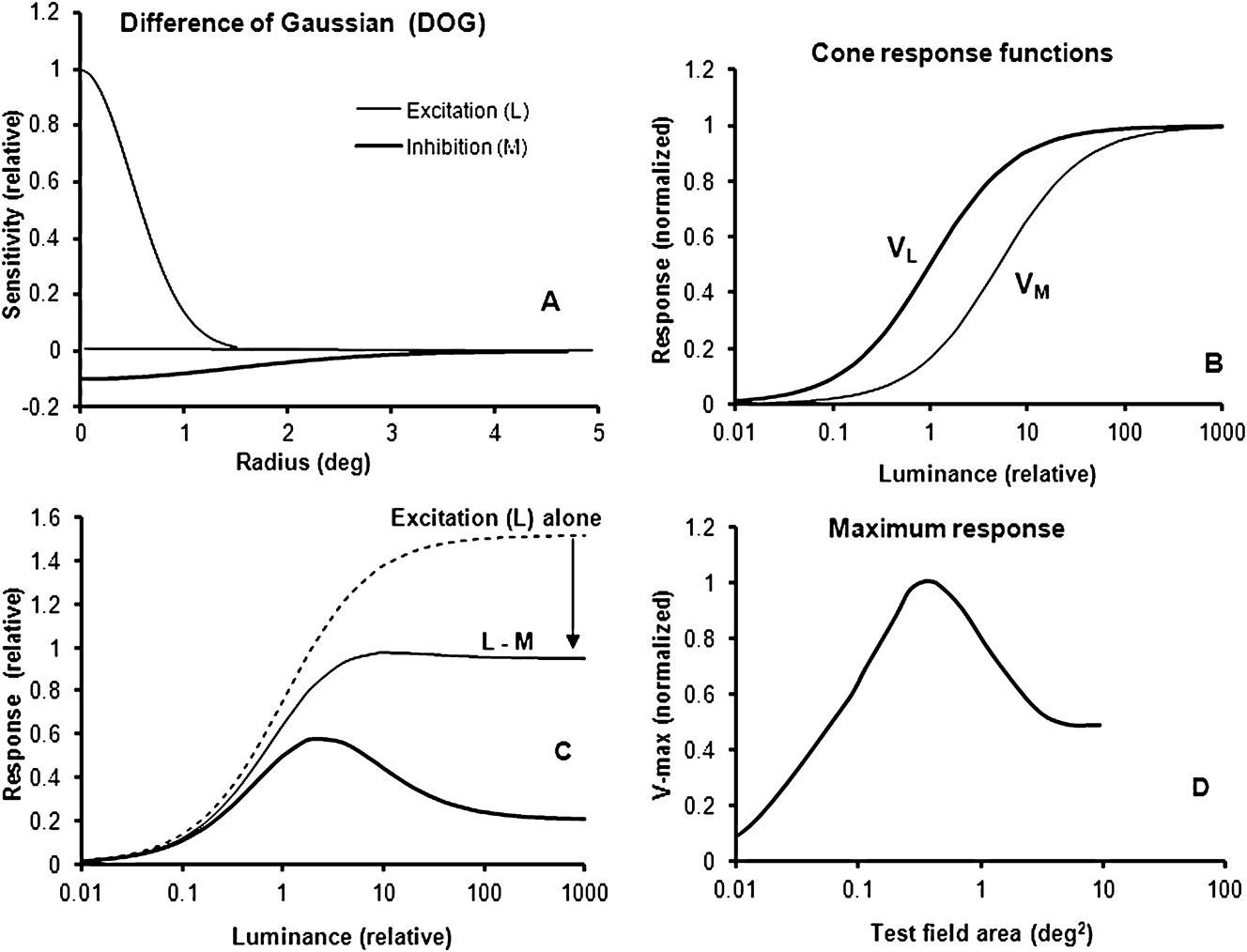
(A) The spatial Gaussian sensitivities of excitation and inhibition of a type I, DOG model, as a function of test field radius. (B) Simulated and normalized L- and M-cone responses V L and V M for a luminance range of 5 log units. (C) Simulated responses for a small and a large test field. For the small spot, within the center of the receptive field, the excitatory L-cone component (broken curve) and the opponent sum of excitatory and inhibitory responses are shown (thin curve). Arrow indicates the magnitude of opponency in the center field. The combination of opponency and suppression for a large test field, covering both the center and the surround of the cell’s receptive field, is shown by the thick curve. (D) For each test field size, the maximum response V max [when the (relative) luminance is varied from 0.01 to 1000] is plotted for test field areas between 0.01 and 100 deg2.

Using data from an earlier study on opponent cells and color coding in the LGN of the macaque monkey (Valberg et al., Reference Valberg, Seim, Lee and Tryti1986, Reference Valberg, Lee and Tryti1987; Lee et al., Reference Lee, Valberg, Tigwell and Tryti1987), we here reanalyse the effect of stimulus size on LGN-cell responses. In these experiments, the luminance range of the test stimulus could span up to 6 log units, and it revealed properties of the cells’ responses that were not observed in experiments with limited ranges of luminance contrast and chromatic saturation (as with gratings on a CRT monitor). The results from this analysis showed that the spatial DOG models (of type I and II) described the cell responses inadequately. The experiments suggested a modified description of responses to homogenous illuminated stimuli where the excitatory/inhibitory balance of opponent cell responses was retained for all stimulus sizes.
In the ECRF, surround suppression affects all cone inputs to receptive field excitation and inhibition equally. It has become customary to model the ECRF suppressive surround by a Gaussian function (Ghosh et al., Reference Ghosh, Sarkar and Bhaumik2005; Crook et al., Reference Crook, Manookin, Packer and Dacey2011), but here we present evidence that ECRF suppression is not compatible with a Gaussian function.
Methods
Preparation
A detailed description of recording procedures may be found in Lee et al. (Reference Lee, Valberg, Tigwell and Tryti1987) and Seim et al. (Reference Seim, Valberg and Lee2012). Briefly, macaques (M. fascicularis) were anesthetized with an intramuscular injection of ketamine hydrochloride (10–20 mg/kg) and further anesthesia was maintained with isoflurane (0.5–1.5%) in a 70/30% N2O/O2 mixture. Electroencephalogram (EEG) and Electrocardiogram (ERG) were recorded as a control for depth of anesthesia, body temperature maintained near 37.5 °C and expired pCO2 kept near 4.5%. All procedures were approved by the Animal Experimentation Committee of the Lower Saxony Government.
Stimulation and recording
The firing rates of cone-opponent PC, koniocellular (KC) and the nonopponent MC cells of the lateral geniculate nucleus (LGN) were recorded in response to achromatic and chromatic stimuli of different sizes, wavelength distribution, relative luminance, and light adaptation. Receptive fields, plotted on the tangent screen, were typically located between 2 and 25° eccentricity. The tangent screen was made of a translucent material for which light transmission was not angular dependent, and stimuli were back-projected upon it. Stimuli were generated by optical means, thus allowing us to explore a 3–6 log unit range of luminance and chromatic variation. Chromatic stimuli of peak wavelengths between 400 and 700 nm were provided by narrow-band interference filters of 50-nm half-maximum bandwidth (Schott). Luminance was controlled by the use of neutral density filters with a flat spectral transmission (Balzers). The test stimulus was usually presented alternating with a white, 110 cd/m2, 4 × 5 deg2 adaptation field, but in some experiments, the white background was left on and the test stimulus was presented upon it. The white adaptation stimulus had CIE chromaticity coordinates (x, y) equal to (0.404, 0.410). When the adapting field was removed, the uniform retinal background luminance was relatively low (ca. 0.9 cd/m2). The test stimuli consisted of eight circular fields between 0.2 and 3.8° diameters, in addition to the square field of 4 × 5 deg2 size. Luminance was computed from the spectral distributions of the stimuli using the CIE V(λ) spectral luminosity function for a 10° field (Lee et al., Reference Lee, Martin and Valberg1988).
To measure intensity–response (I–R) curves, the intensity of the test stimulus was increased in 10 steps, covering a 3-log-unit range of luminance so that each luminance increment was approximately 0.3 log units. The total range was sometimes extended to 6 log units by using appropriate neutral density filters. The extended range usually reached from 3 log units darker to 2 log units brighter than the adaptation field. The response is plotted as a function of luminance ratio Y (luminance of the test field divided by the luminance of the background).
Before and between each presentation of the test field, the adaptation field (A) was presented for 1200 ms. The maintained firing rate of the cell is then N A imp/s. When the adaptation field was replaced by a brighter or darker test stimulus (T) of 300-ms duration, a cell’s firing changed to N T imp/s. Our response measure was the difference response, N T − N A, that is, the change in firing rate when the white adaptation field was replaced by the test stimulus. For test spots smaller than the 4 × 5 deg2 background, this means that the test field appeared on a dark (ca. 0.9 cd/m2) background, except in experiments where the white adapting field A was left on. This latter condition was always used for transient MC cells.
The response magnitude N T during test field presentation was defined as the mean sustained firing rate within a 240-ms window following a 45-ms period after the onset of the 300-ms test stimulus. To avoid possible artifacts, the 45-ms transient interval was excluded from the analysis, except when the transient responses of MC cells were analyzed. Bin-width was 15 ms. Each I–R recording sequence was repeated 10 times, and the data, presented here, are the average of these 10 presentations.
Modeling LGN cell responses
In the model (Seim et al., Reference Seim, Valberg and Lee2012), we use a weighted opponent combination of cone output signals, V L, V M, and V S to describe the response of an LGN cell:
 $${N_{{\rm{LGN}}}} = \pm {\rm{ }}{A_{\rm{L}}}*{V_{\rm{L}}} \pm {A_{\rm{M}}}*{V_{\rm{M}}} \pm {A_{\rm{S}}}*{V_{\rm{S}}} - {N_0},$$
where A L, A M, and A S are amplitude weighting constants. For typical “L–M” PC cells, we can write
 $${N_{{\rm{LGN}}}} = {A_{\rm{L}}}*{V_{\rm{L}}}{\rm{ }} - {A_{\rm{M}}}*{V_{\rm{M}}} - {N_0}.$$
The receptor hyperpolarization evoked by light can be described by the hyperbolic Naka–Rushton formula:
 $${V_{\rm{M}}} = {M^n}/({M^n} + {\sigma ^n}_M{\rm{),}}$$
for the M-cone, and similarly for responses V L and V S of the two other cone types. L, M, and S represent the amount of light absorbed by the L-, M-, and S-cone, respectively. They are the integrals over wavelength of the spectral emission of the light stimuli multiplied by the cone fundamentals (Stockmann & Sharpe, Reference Stockmann and Sharpe2000). The constant σ is the light absorption at half-saturation, with a different value for each cone type. The exponent n is allowed to vary between 0.7 and 1.0 (Valeton & Van Norren, Reference Valeton and Van Norren1983). The introduction of an activation threshold N 0 for the LGN cell (Seim et al., Reference Seim, Valberg and Lee2012) implies that the activity of the afferent ganglion input to the LGN cell must reach this threshold value before the LGN output is activated.
When I–R curves are plotted using luminance along a logarithmic x-axis, changes in the cell’s sensitivity result in horizontal shifts of the I–R curves. Changes in responsiveness result in an amplification or attenuation of the I–R curve. In the model, the cell’s sensitivity is represented mathematically by the cone half-saturation constants σ, whereas its responsiveness is represented by the amplitudes A. This way of defining sensitivity deviates slightly from the more commonly used, where only the position on the x-axis of a single point (the threshold value) on the response curve is used.
The DOG model
For a DOG model type I “L–M” ganglion cell, the spatial extent of excitation and inhibition of the receptive field is shown in Fig. 1A as a function of the distance r to the receptive field center. The general Gaussian function is
 $$g(r) = A*{e^{ - \alpha {r^2}}},$$
where A and α are constants and r is the radius. In the figure A L = 1, A M = − 0.1, α L = 2, and α M = 0.23. The center of the receptive field of this “L–M” cell is defined as the area where the L-component, represented by g(r, L), is present. For the DOG type I model, the size of the inhibitory field is always larger than that of the excitatory field. In Fig. 1A, the center radius is 1.5° and the center area is 7.07 deg2. (theoretically a Gaussian function never reaches zero response for larger areas, but it quickly falls below 1/1000 of maximum value).
Fig. 1B shows the normalized cone input signals V M and V L to the opponent ganglion cell when we use the hyperbolic function of eqn. (2) to compute the excitatory and inhibitory input signals from the L and M cones. When an excitatory wavelength for the L-cone is selected, for example, 620 nm, the simulated excitation of this cone will be larger than that of the M-cone (see Fig. 1B, where σ L = 1, σ M = 5, and n = 1). The DOG type I spatial response can be modeled as
 $$N = g(r,L)*{V_{\rm{L}}} - {\rm{ }}g(r,M)*{V_{\rm{M}}}.$$
Fig. 1C shows the simulated cell response as a function of luminance for a test field size equal to the classical center of the receptive field (thin curve) and for a larger test field covering both the classical center and the surround of the cell (thick curve). The excitatory L-response to the small test spot is also shown (dashed curve). Since the excitatory L-component is more sensitive than the inhibitory M-cone, it will dominate the response at low luminances, but for increasing luminance, the sum of inhibition and excitation makes the response curve first reach a maximum and then to become attenuated at still higher intensities (thin curve). When the luminance of the stimulus is approximately 2 log units higher than the cell’s threshold (around 0.01 in the figure), the response curve is attenuated by the inhibitory component (M), as indicated by the arrow. For the large test field (thick curve), covering the entire receptive field of the cell, the DOG response at higher luminance decreases strongly due to the increased influence of the inhibitory component in the surround field.
The predicted maximum responses for test fields of increasing size are shown in Fig. 1D. For each test field size, we computed the maximum response when the (relative) luminance varied from 0.01 to 1000. This maximum response (V max) is plotted in Fig. 1D for test field areas between 0.01 and 100 deg2 (diameter 0.056 and 5.6°). At low luminance, the V max amplitudes increase when the size of the test field increases and reach a maximum for r = 1.1° (area = 3.8 deg2 or about half the area of the receptive field center). For larger r, the maximum amplitudes decrease until the test field becomes larger than for the inhibitory surround, where V max is constant.
Results
Only responses of ON-cells are presented in this work. We are using the Increment (I-cell) notation because it points out to the role of these cell types in discriminating graded luminance and chrominance dimensions of light stimuli (Valberg & Seim, Reference Valberg and Seim2008).
Large test fields
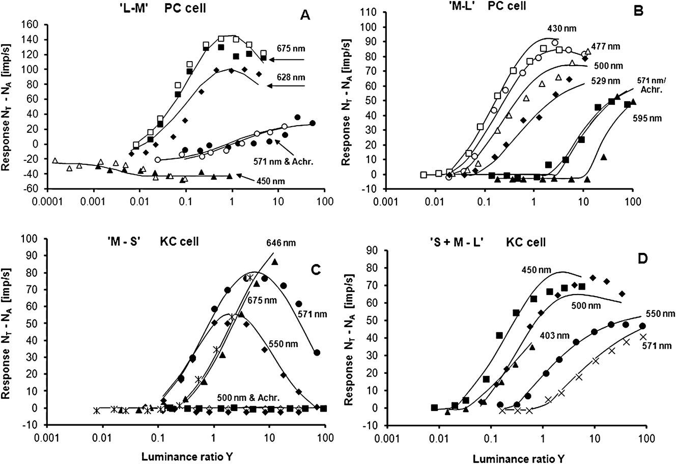
The large-field experiments consisted of a 4 × 5 deg2 adaptation field, shortly replaced by a test field of the same size. This size ensured coverage of both the center and the surround of the cells’ CRFs at the eccentricities involved (Lee et al., Reference Lee, Valberg, Tigwell and Tryti1987; Valberg et al., Reference Valberg, Lee and Tryti1987). Measured responses, together with responses derived from using eqn. (1), are presented in Fig. 2A–2D. These figures display the responses of typical cone-opponent-coding I-cells when they were stimulated with different chromatic and achromatic test fields. For the two PC cells (“M–L” and “L–M”) shown in Fig. 2A and 2B, the responses to achromatic light and 571-nm yellow light (which represents the spectral zero crossing for pure “L–M” and “M–L” cells) are equal, indicating that neither of these cells had S-cone input. In Fig. 2C, the response of a KC I-cell with subtractive S-cone input is shown, and Fig. 2D displays the recorded I–R curves and the model fit for a KC cell with excitatory S-cone input. To give an example of reproducibility, the responses of the cell in Fig. 2A to the 675- and 450-nm stimuli were measured twice.
(A) Measured and simulated responses for a PC, “L–M” LGN Increment cell. Abscissa: luminance ratio Y = (luminance of test field)/(luminance of background). Test and adaptation field sizes: 4 × 5 deg2. Luminance range: approximately 6 decades. Curves and symbols represent simulated and measured responses to different wavelengths and an achromatic light (filled circles). A common set of parameters in eqn. (1) is used to model all spectral and achromatic responses. For 450 and 675 nm, two measurement series are shown in order to give an impression of typical reproducibility. Wavelengths refer to maximum transmission of the narrow band interference filters. Cell: E10U15. (B) Simulation and responses of a PC, “M–L” LGN I-cell, a common fit for all data. The responses for the achromatic and the 571-nm test stimuli (neutral wavelength) merge, indicating no S-cone contribution. Cell: E07U21. (C) Same as Fig. A and B for a KC, “M–S” Increment cell, the responses to achromatic (and green) stimuli were strongly attenuated due to opponency, as expected from simulated response curves. Cell: E17U1B. (D) Same as above. Simulation of responses of a KC, “S + M–L” Increment cell compared with recorded I–R curves. Cell: E14U04.
For all spectral stimuli of Fig. 2A–2D, the model fits of eqns. (1) and (2) (solid curves) closely follow the data points of the I–R curves. By using eqn. (1), we obtain satisfactory descriptions of the recorded responses over the whole luminance range of up to 6 log units. This large luminance range brings out nonlinear properties of the LGN cell responses. For example, at low intensities, the “L–M” cell’s response to the 675-nm test stimulus (Fig. 2A) is dominated by input from the excitatory L-cone component. When the luminance increases to about 2 log units above threshold, it becomes high enough to activate the inhibitory M-cone. For still higher intensities, the excitatory L-response saturates, whereas the inhibitory M-component keeps on increasing, and the cell’s response decreases. For the PC, “M–L” cells (Fig. 2B), excitation by M-cone and inhibition through L-cone inputs behave in a similar way for the excitatory 477-nm stimulus. The amplitudes of the “M–S” cell in Fig. 2C display a pronounced contribution from the inhibitory cone.
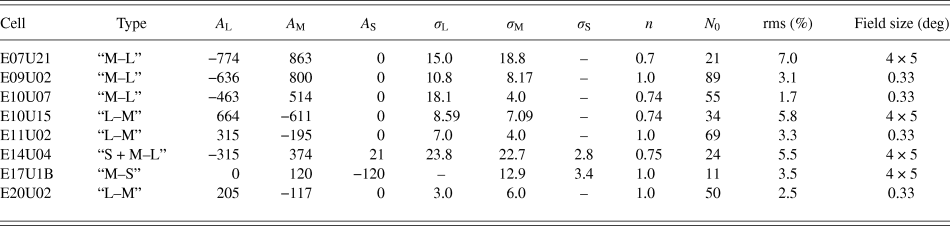
The precise fits by a single set of constants in eqn. (1) of the cells’ responses to stimuli of many wavelengths over a 6-log-unit luminance range demonstrate the reliability of the model in describing the spectral and luminance dependent behavior of PC and KC cells. We have described such large field multispectral response modeling earlier (Valberg et al., Reference Valberg, Lee and Tryti1987), but the introduction of an activation threshold for the LGN response (Seim et al., Reference Seim, Valberg and Lee2012) has significantly improved the fits. Although the old model had a target of obtaining a relative rms error of 10% for the cells response simulations, the average rms for the four fits, displayed in Fig. 2 for the new model, is 5.5% of maximum firing rate. Model parameters and rms values are shown in Table 1.
Model parameters obtained by using eqn. (1) on eight opponent LGN cells. The first column displays the cell number, whereas the second presents the cone opponency. The parameters of eqn. (1), leading to optimal fit with data, are found in the next eight columns. The relative rms errors are also shown, together with the diameter of the test field
These results can be compared with the outcome of a DOG-type model for a large test field, covering both the center and the surround field, as shown in Fig. 1C (thick curve). With a fixed-size stimulus, the spatial sensitivity profile of the cell is not relevant, only the luminance–wavelength dimension, for which there is no specific Gaussian profile. Since we have introduced the Naka–Rushton function in both models [eqn. (2)], we can compare the DOG model with the new model responses in Fig. 2 (black curves). The strength of the excitatory and inhibitory components for both models is represented by the A-values in Table 1. For I-cells, the response magnitude of the excitatory component is always larger or equal to that of the inhibitory amplitude. This is in agreement with what was found in previous simulations of I-cells (Valberg et al., Reference Valberg, Lee and Tryti1987).
Test fields of different sizes
For the results presented above, the size of the test and the adaptation field was 4 × 5°. In the experiment described below, a circular test spot varied in diameter from 0.2 to 3.8°.
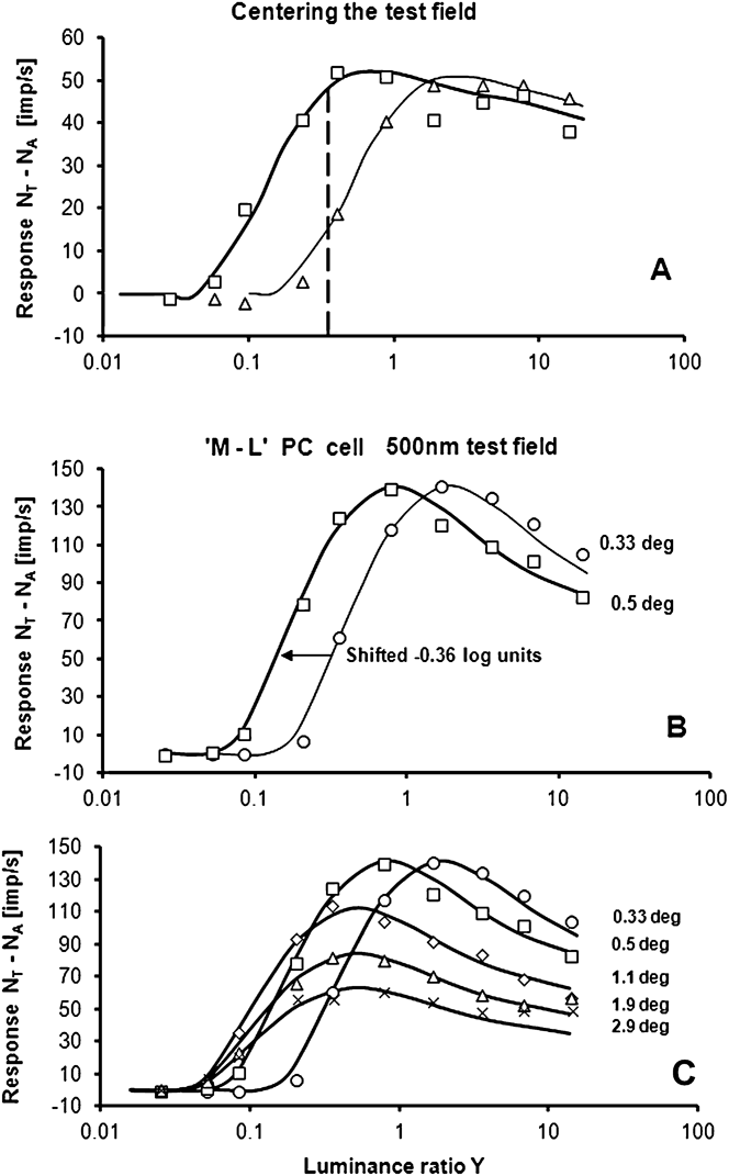
Care was taken to center the test field properly on the center of the receptive field. How this was done is demonstrated in Fig. 3A. When the 0.33° test field was centered on the receptive field, the sensitivity of the cell was optimal and the response curve reflected maximum sensitivity to luminance increments (thick curve). When the test field was moved slightly away from the center, the sensitivity decreased (thin curve). The stability of fixation could be controlled by repeated stimulations, each consisting of 10 measurements of the whole I–R curve. This method can be compared with another one, using a test field with constant luminance, indicated by the vertical broken line in the figure. This method yields optimum centering when the response is highest. Both methods can be used for centering, but the precision is higher when responses to 10 luminances, not only one, are used for finding the center position.
(A) Centering of the test spot on the receptive field center of an “L–M” I-cell. Optimal centering is obtained when the I–R curve is in the leftmost position (thick curve). The vertical dashed line shows the response to the two spot positions when the test luminance ratio is constant. Test spot: 0.33° diameter. Cell: E11U02. Wavelength: 675 nm. (B) I–R curves for test fields with diameters of 0.33° (circles) and 0.5° (squares). When size increases, the I–R curve shifts horizontally to the left, without changing shape. Note that the maximum response is maintained. Response curves are simulated by eqn. (1). Cell: E09U02. (C) Measured responses and simulated I–R curves for five sizes of a 500-nm test field.
We have measured the responses of 53 LGN I-cells (33 PC, 8 KC, and 12 MC cells) to different test field sizes, intensities, and wavelengths. To describe how these cells responded to test fields of varying size and luminance, we have selected a representative PC cell in Fig. 3B and 3C. Based on the responses to six different wavelengths within a 0.33°-diameter field, this cell was defined as an “M–L” I-cell. Of special interest are the responses of this cell for the two smallest (0.33 and 0.5° diameter) test fields. These are shown in Fig. 3B for an excitatory 500-nm stimulus. For the 0.33° test field, the model fit (thin curve), closely follows the data (circles). Shifting this curve to the left (thick curve) gives a good description of the responses to the 0.5° test field (squares). The model parameters are given in Table 1.
As explained for Figs. 1 and 2, the excitatory (M-cone) input dominates the response at low intensities, whereas the opponent (L-cone) input causes a response decrease at higher intensities. Since the response curves to the 0.33 and 0.5° fields have the same form, the sensitivity of the excitatory and the inhibitory components have, according to eqns. (1) and (2), changed by the same factor.
Fig. 3C shows that the maximum values of the I–R curves are increasingly reduced for test diameters beyond 0.5°. The responses to five test fields of different diameters are displayed, together with the model fits. The model curves have been generated simply by horizontally shifting and attenuating the I–R curve for the 0.33° test field. As can be seen from the figure, this procedure gives a nice account for the I–R curves for all of the other test field sizes. A common basic curve also implies that both amplitude ratios A L/A M and the ratios of half-saturation constants σ L/σ M are constant in eqns (1) and (2). Constancy of these ratios across stimulus sizes was an empirical result, but it turns out to be a necessary prerequisite for color stability of stimuli of the same chromaticity and luminance factor. This will be further elaborated in the Discussion section.
As for the responses based on a DOG model, shown in Fig. 1C, the shape of the response curve is expected to change when the size of the test field is increased from a small spot to a large one. In Fig. 1C, the amplitude of the I–R curve for large spots decreases, but mainly for high luminances. In contrast to this prediction of a DOG model, and as shown in Fig. 3C, the entire curve is attenuated by a constant factor for large fields.
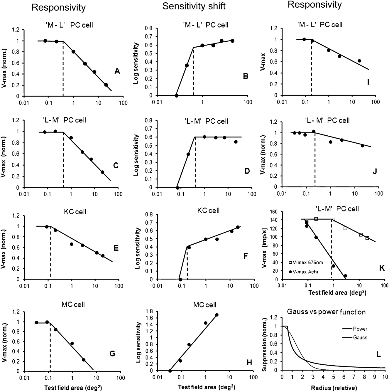
For the responses displayed in Fig. 3C, Fig. 4A shows the responsiveness of the cell represented by the maximum response V max as a function of the logarithm of test field area. V max data are normalized to 1.0 for the smallest (0.33°) field. Measured, not modeled, values are shown. In Fig. 4B, the sensitivity of the cell, as a function of size, has been derived from the five I–R curves in Fig. 3C. As ordinate in Fig. 4B, the sensitivity is plotted on a logarithmic scale. Since increasing sensitivity leads to a leftward shift of the I–R curves, −∆log (Y) is plotted along the ordinate and normalized to 0 for the smallest test spot.
(A) The maxima (V max) of the I–R curves for the opponent “L–M” cell are plotted for each of the five test field sizes in Fig. 3C. In the center region (marked by the broken vertical line), the cell’s maximum responsiveness is constant. Outside the center region, the suppression of maximum response follows a straight line with negative slope when plotted as a function of the logarithm of the test field area. (B) Sensitivity of the cell in Fig. 3C, plotted as a function of test field area. The increase in sensitivity when the area is increased from 0.33 to 0.5° indicates area summation. Increasing sensitivity leads to a leftward shift of the I–R curves. Log sensitivity is defined as −∆log (Y) and plotted along the ordinate (normalized to 0 for the smallest test spot). The size of the center region can be determined by two independent methods (broken vertical lines in 4A and 4B). Both methods give about the same size. Cell: E09U02. Eccentricity: 14°. (C) V max variation for an “M–L” opponent cell, plotted as a function of the test spot area. The result is similar to the “L–M” PC cell shown in 5A. (D) Sensitivity plotted as a function of the test field area for this “M–L” cell. For this particular cell, the sensitivity is constant, not increasing in the surround field. Cell: E09U01. Eccentricity: 14°. (E) V max for a 450-nm stimulus, plotted as a function of the log area for a KC cell. (F) Sensitivity of the same cell plotted as a function of the test field area. The size of the center field and the response in the surround field is similar to that of a PC cell. Cell: E09U08. Eccentricity: 12°. (G and H) Similar plots for a MC cell for an achromatic test stimulus. The surround suppression for MC cells is stronger than that for PC and KC cells. In addition, the sensitivity variation in (H) is linearly dependent on a log area. Cell: E22U51. Eccentricity: 17°. (I and J) Maximum responsivity V max as a function of the test field area for two other PC cells. The slopes (suppressive strengths) in the surround of PC cells varied considerably. The additional two cells are E10U14 (eccentricity 5°) and E15U05 (eccentricity 7°). (K) When plotting V max as a function of log area of “L–M” PC cells, the stipulated size of the center decreases when the excitatory (675 nm) stimulus is replaced with an achromatic stimulus. The size of the center then becomes smaller than the smallest test field used. Cell: E10U0. Eccentricity: 7°. (L) Comparison of spatial suppression predicted by a Gaussian-shaped function (thin curve) and a power function (thick curve).
One method of assessing the receptive field center is the area-threshold method (Barlow et al., Reference Barlow, Fitzhugh and Kuffler1957; Wiesel & Hubel, Reference Wiesel and Hubel1966; Peichl & Wässle, Reference Peichl and Wässle1979; Crook et al., Reference Crook, Lange-Malecki, Lee and Valberg1988). This method is used in Fig. 4B, but sensitivity (equal to 1/threshold) not threshold is plotted as an ordinate. By plotting sensitivity on a log scale, log(sensitivity) = −log(threshold) and the shape of the threshold curve is inverted but not changed. The sensitivity data reveal two regions of sensitivity change: one for small stimulus sizes, where the sensitivity increases steeply with size, and another where the increase is absent or more shallow. The crossing of the two linear regressions (indicated by the vertical dashed line) is our definition of receptive field center area. Measuring threshold sensitivity as a single point on the response curve, or using the entire I–R curve, leads to similar results, as described in Methods.
An alternative method for defining the receptive field center is shown in Fig. 4A, where the responsiveness is fairly constant for small stimulus sizes (see also Fig. 3B). At larger stimulus sizes, the responsiveness decreases proportional to the logarithm of the stimulus area. The crossing of the two linear regressions in Fig. 4A may be used to define the size of the center field (indicated by the vertical dashed line). Both methods lead to similar sizes of the receptive field center. According to the model described by eqn. (1), both the excitatory and the inhibitory components of cone opponency are present in the center and constant responsiveness applies for the smallest stimulus sizes used.
In the work of Seim et al. (Reference Seim, Valberg and Lee2012), similar responses to those shown in Fig. 3C are plotted for an “L–M” I-cell (see their Fig. 7). Also for this cell, a common curve, shifted and/or attenuated, describes this cell’s responses to the same five test fields. Fig. 4C confirms the logarithmic relationship between V max and area. Fig. 4D shows that the sensitivity can be close to constant in the surround, unlike the cell shown in Fig. 4B.
Fig. 4I–4IJ show the responses for two extra cells, selected to demonstrate the variability of suppression in the surround. Compared to the “L–M” and “M–L” cells in Fig. 4A and 4C, these two cells behave in a similar manner but show less suppression in the surround; even zero suppression was found for some PC cells. When the steepness of the slopes (strength of suppression) for all 33 PC cells are plotted as a function of eccentricity, the variation of the slopes appears to be largely independent of the cells’ eccentricity. Fig. 4J shows that the responsivity in the center field was close to constant for the smallest test fields (0.2 and 0.25° diameter) used in the experiment.
Surround suppression
Fig. 4A and 4C demonstrate that outside the center of the receptive field (within which the cell’s maximum responsiveness, V max is close to constant), the suppression of V max follows a logarithmic function of test spot area. It can be described by the equation
 $${V_{\max }} = - {\rm{ }}a * {\rm{log}}(\varphi ) + b,$$
where  ${\rm{log}}(\varphi )$ is the logarithm of the test spot area φ, and a and b are constants. When the cell’s maximum responsiveness V max within the center field is normalized to 1.0, then eqn. (5) is valid for V max ≤ 1.0. When the constants a and b are known, the size of the center field can be computed by calculating the value of φ for V max = 1. The size of the test field area where the response becomes completely suppressed is found by setting V max = 0. Using eqn. (5) on the cell responses shown in Fig. 4A and 4C results in center areas of 0.36 and 0.53 deg2 (or diameters of 0.68 and 0.82°) and complete suppressive areas of 61 and 82 deg2 (diameter 4.4 and 5.1°), respectively.
In order to compare this result with the response predicted from a DOG function as in Fig. 1A, we must compute the suppression sensitivity as a function of the radius of the test field. Fig. 4A shows that suppression (Sup) takes place outside the center field with radius r c. For the smallest test spot sizes used, no notable suppression was seen in the center field. The attenuation outside r c, as a function of radius, can then be found (if we assume linearity) by derivation of eqn. (5), leading to the power function
 $${\rm{Sup}} = k * {r^\varepsilon }{\rm{when }}r \ge {r_{\rm{c}}},$$
where r is the radius of the test field, the exponent ε = −1 and k is a constant. Combining eqn. (1B) for the “L–M” cone opponency (or any other cone opponency) and eqn. (5) for spatial suppression, we obtain:
 $${N_{{\rm{LGN}}}} = ({A_{\rm{L}}} * {V_{\rm{L}}} - {A_{\rm{M}}} * {V_{\rm{M}}} - {N_0}) * ( - a * {\rm{log}}(\varphi ) + b),$$
when r > r c and  $- a * {\rm{log}}(\varphi ) + b$ is replaced by 1 when r ≤ r c. In this equation, the separate mechanisms of the classical subtractive opponency and the extraclassical multiplicative surround suppression become clearer; each parenthesis represents the separate mechanisms, the first one being additive and the second one multiplicative. This equation accounts for the spatial suppression and spectral response of our new model.
To compute the changes in sensitivity seen in Fig. 3C, eqn. (2) must be expanded. Here the sensitivity of the M- and L-component is proportional to 1/σ M and 1/σ L, respectively. For the I–R curve of the “L–M” opponent to change its sensitivity, without changing the shape of the I–R curve, both 1/σ L and 1/σ M must be multiplied by a common constant c. (Making c equal to 2.0 will make the I–R curve twice as sensitive). Eqn. (2) is then changed to
 $${V_{\rm{M}}} = {M^n}/({M^n} + {({\sigma _{\rm{M}}}/c)^n}),$$
for the M-cone, and similarly for response V L of the L cone. When sensitivity increases with area, this can be described by
 $$c = d * \varphi + e,$$
where φ is the test spot area and d and e are constants. If the sensitivity increases linearly with the area of the test spot in the center region, then d = 1.0. If the sensitivity is constant in the surround area, like in Fig. 4D then d = 0 here, otherwise 0 < d < 1.0. Eqns. 7A–7C give a complete mathematical description of the response curves shown in Figs. 3C and 4A–4D.
Center area summation
By increasing the test field from 0.33 to 0.5° (from 0.086 to 0.20 deg2), the sensitivity of the cell in Fig. 4B increased by 0.36 log units or by a factor of 2.3. The test field area increment, going from 0.086 to 0.20 deg2, is also 2.3. The summation factor (increase in sensitivity divided by increase in area) is thus 1.0, making the constant d equal to 1.0 in eqn. (7C). For the cell in Fig. 4D, the sensitivity increases about 0.4 log units (or 2.5 times) when the spot diameter increased from 0.33 to 0.5°, equivalent to an area summation factor of 1.09. For 15 PC cell recordings, where at least two test fields were smaller than the putative receptive field center, the average summation factor was 1.04 ± 0.2, with maximum 1.6 and minimum 0.7. This is close to what Peichl and Wässle (Reference Peichl and Wässle1979) found in cat retina and what Crook et al. (Reference Crook, Lange-Malecki, Lee and Valberg1988) found in the macaque. This is not compatible with a theoretical Gaussian sensitivity curve for which the summation factor is always less than 1.0 [i.e., close to 0.8 according to Peichl and Wässle (Reference Peichl and Wässle1979)].
The results presented above are all for excitatory chromatic stimuli. For six PC cells, achromatic lights or neutral wavelengths (e.g., 571 nm for PC cells) were also applied as test stimuli. The center sizes estimated from several of these recordings were smaller than the smallest test field used, as demonstrated for a “L–M” cell in Fig. 4K. This means that the area of the center size was reduced by 1 log unit or more for achromatic lights (or neutral 571-nm wavelengths). These results demonstrate that the area of summation, or receptive field center, was strongly dependent on the spectral properties of the stimulus.
Summary of receptive field properties of PC cells
For 23 of the 33 PC I-cells we have analyzed, a common curve, shifted and/or attenuated, could be used to model the I–R responses as a function of stimulus area (similar to Fig. 3B–3C). For five cells, a common (shifted) curve could be used to model the responses in the center.
For 26 PC cells, a close to linear dependency of V max on log area was found outside the receptive field center.
Of the 33 PC cells, the V max of four cells could not be analyzed due to a missing response maximum as a function of luminance. Of the remaining 29 cells, 15 displayed a nearly constant V max in the center for at least two stimulus sizes (five with three spot sizes in the center). Eight cells were tested with only one test spot within their center (recognizable because the V max for the smallest stimulus size was below the linear regression); the size was estimated from the combined analysis of V max and sensitivity shifts (like in Fig. 4A and 4B). For six cells, the smallest test spot used was larger than the center (because a linear regression of V maxvs. stimulus area could describe all data well). Four cells had close to constant V max for all test spot sizes, indicating a weak or absent surround suppression.
Spot sizes below 0.33° diameter were used for less than 50% of the cells due to difficulties with keeping the test field centered. Another possible reason might be found in the work of Webb et al. (Reference Webb, Tinsley, Vincent and Derrington2005) who showed that the shape of the receptive field centers can be asymmetrical.
The sensitivity shifts of the surround are illustrated in Fig. 4B and 4D. The sensitivity either increased slightly (Fig. 4B) or remained constant for increasing test field sizes, i.e., for approximately 70% of the cells.
Receptive field profiles of other cell types
For six KC cells with excitatory S-cone input, the surround suppression of V max also followed a logarithmic function. A typical result is presented in Fig. 4E and 4F. This cell responded in a way similar to that of the PC cells shown in Fig. 4A and 4B. In Fig. 4F, the sensitivity of the KC cell increases in the surround-field (as does the “M–L” cell in Fig. 4B). This was unexpected, since other threshold experiments on ganglion cells usually show close to constant surround sensitivity (Peichl & Wässle, Reference Peichl and Wässle1979, Crook et al., Reference Crook, Lange-Malecki, Lee and Valberg1988). However, the experiment performed by Wiesel and Hubel (Reference Wiesel and Hubel1966) showed similar behavior for a KC cell (their Fig. 9).
Only two KC cells with inhibitory S-input have been analyzed. Both cells responded in a similar way, but contrary to the other cell types presented above, their maximum responsiveness increased when the test field area increased within the center field. Outside the center field, the response was logarithmically suppressed, as found for the other cell types.
Transient responses of 12 MC ON-neurons have also been studied. All MC cell recordings were made using achromatic test stimuli presented upon a steady background. The result for one typical cell is shown in Fig. 4G and 4H. All 12 cells responded like that shown in Fig. 4G. The size of the center fields, defined as having constant V max, was less than approximately 0.35 deg2. The logarithmic attenuated slopes for stimulus sizes larger than the center field of the MC cells were steeper than for the PC cells, indicating that surround suppression was stronger for MC cells.
Except for 1 cell (out of 12), the sensitivity increased linearly, as shown in Fig. 4H, with an average slope of 0.60. The correspondence between the two methods used for defining the center size (Fig. 4A and 4B) was not seen for the transient responses of MC cells.
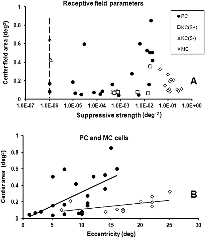
In Fig. 5, we summarize the results for the different cell types. In Fig. 5A, the size of the center for all cell types is plotted as a function of the strength of surround suppression. As a measure of the suppressive strength, we use the inverted value of the (extrapolated) test-field area, where the responsivity becomes zero [by using eqn. (5) with V max = 0]. Note that the MC cells possess the strongest surround suppression, whereas the two KC(−S) cells have the weakest. The vertical dashed line indicates the practical limit of the weakest suppressive strength. The KC(S+) cells show less variation in suppressive strength than PC cells. The figure shows that the suppressive strength for PC cells has a maximum value around 0.022 deg−2, whereas the maximum value for MC cells is more than ten times larger, approximately 0.34 deg−2.
(A) Center sizes as a function of the suppressive strength for all cell types. Suppressive strength is defined as the inverted value of the (extrapolated) test field area where the responsivity becomes zero [by using eqn. (5) with V max = 0]. The vertical broken line indicates a reasonable lower limit of suppressive strength. (B) The size of the center field of PC cells (circles) tends to increase with eccentricity, indicated by the trend line, as does the size of the center field of MC cells (diamonds). The sizes of the center fields of MC cells are smaller than for PC cells at all eccentricities.
In Fig. 5B, the sizes of the receptive center fields of PC and MC cells are plotted as a function of foveal distance (eccentricity). The center size of PC cells tends to increase with eccentricity, indicated by the linear trend line in the figure, but there is substantial scatter in the data. The center size of MC cells shows a similar trend, but in general, the sizes are smaller than for PC cells. This was surprising for several reasons since the dendritic fields of MC-type ganglion cells are larger than those for PC cells (De Monasterio & Gouras, Reference De Monasterio and Gouras1975; Watanabe & Rodieck, Reference Watanabe and Rodieck1989). However, the size of the center found in our experiment is much larger than what can be assumed based on dendritic fields of bipolar and ganglion cells (see Discussion).
Source of suppression
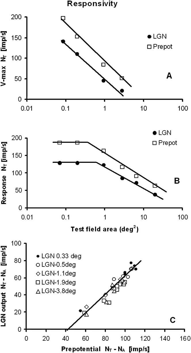
Although a LGN cell sensitivity and its activation threshold N 0 (eqn. 1) can be influenced by cortical feedback and by interneurons in the LGN (Seim et al., Reference Seim, Valberg and Lee2012), the suppressive surround for opponent PC-cells in the LGN is probably mainly generated by the retinal inputs to these cells (i.e., the retinal ganglion cells). This can be deduced from simultaneous measurements of prepotentials and LGN cell responses (Fig. 9, Lee et al., Reference Lee, Virsu and Creutzfeldt1983). In Fig. 6A, the V max values of a PC I-cell (filled circles) and its prepotentials (squares) are plotted as a function of the area of an achromatic test field. The magnitude of the maximum responsivity of the suppressive surround of the LGN cell and the retinal ganglion cell can be both approximated by similar logarithmic functions.
(A) Surround suppression is also seen in the prepotentials to the LGN cell, indicating a retinal origin of the suppression of the LGN response. Cell: E10U01. Eccentricity: 7°. (B) Using eqn. (1), the prepotential is computed from the recorded LGN I–R curve of a PC I-cell. Surround suppression for the computed prepotential, as a function of the test spot area, is similar to that of the LGN response. Cell: E09U01. Eccentricity: 14°. (C) The linear relationship between the LGN cell output and its prepotential, previously shown for stimuli of different colors (Lee et al., Reference Lee, Virsu and Creutzfeldt1983), also applies for test fields of different areas. Cell: E11U04. Eccentricity: 2°.
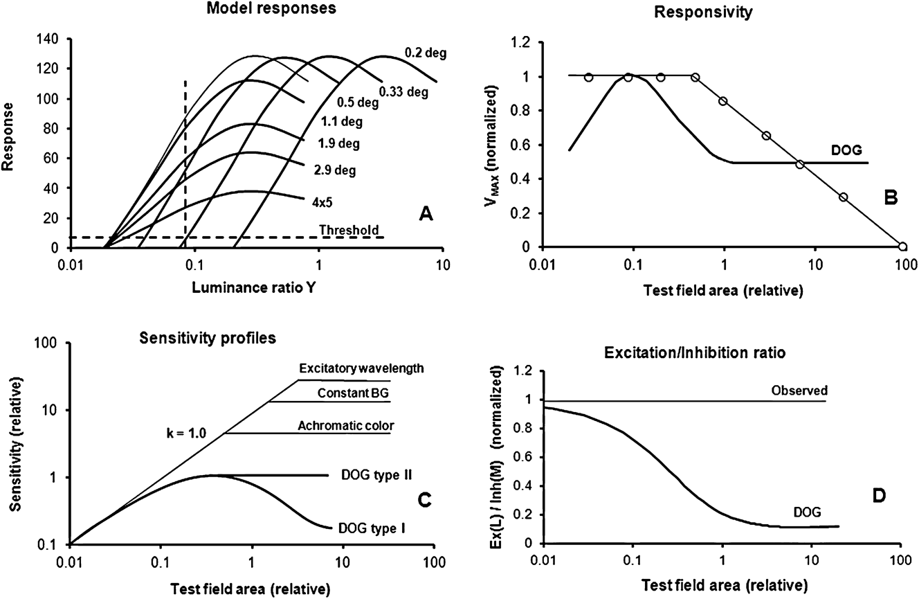
(A) Simulated I–R curves for a typical opponent PC cell to test fields of increasing size. Two different methods for determining the size of the center field are also shown. The use of a luminance threshold method and a constant luminance method is indicated by the horizontal and the vertical dashed lines, respectively. (B) The responsivity, computed from a DOG model (thick curve), is compared to that of the model represented in Fig. 7A (open circles). For small test spots, the DOG shows low maximum responses, while the measured responsiveness is close to constant within the center-field area. The logarithmic attenuation for larger test fields is not compatible with the DOG model. (C) This figure summarizes the differences in response sensitivity for the DOG and the new model. The modeled sensitivity profile for homogenous stimuli is shown, together with the spatial sensitivity profiles of the two DOG models. For small homogenous test fields, the measured sensitivity increases linearly with log area, indicated by the line with slope k = 1.0. A slope of 1.0 indicates that linear summing takes place, achieved by using d = 1.0 in eqn. (7C). In the new model, the sensitivity reaches a constant value for fields larger than the center field. Constant sensitivity is obtained when c is constant in eqn. 7C. Three examples are shown: For excitatory wavelengths, the size of the center field is large, as shown in the figure. Replacing the excitatory test color with an achromatic stimulus significantly reduced the size of the center field (see response labeled Achromatic color). When the background was constant on (labeled Constant BG), then the size of the center field became reduced compared with what was found for excitatory test colors with alternating backgrounds. The DOG type I and II models (thick curves) do not show linear summation of sensitivity within the center field. (D) The ratios between the excitatory (L) and inhibitory (M) components are plotted as a function of the test field size for the DOG model (thick curve) and the model of Fig. 7A (thin line). Contrary to our experimental results, for the DOG model, the ratios become smaller with increasing size of the test spot. Experimentally, however, little or no change is found for responses to homogenous stimuli, as expected from every-day experience with color perception and psychophysical observations.
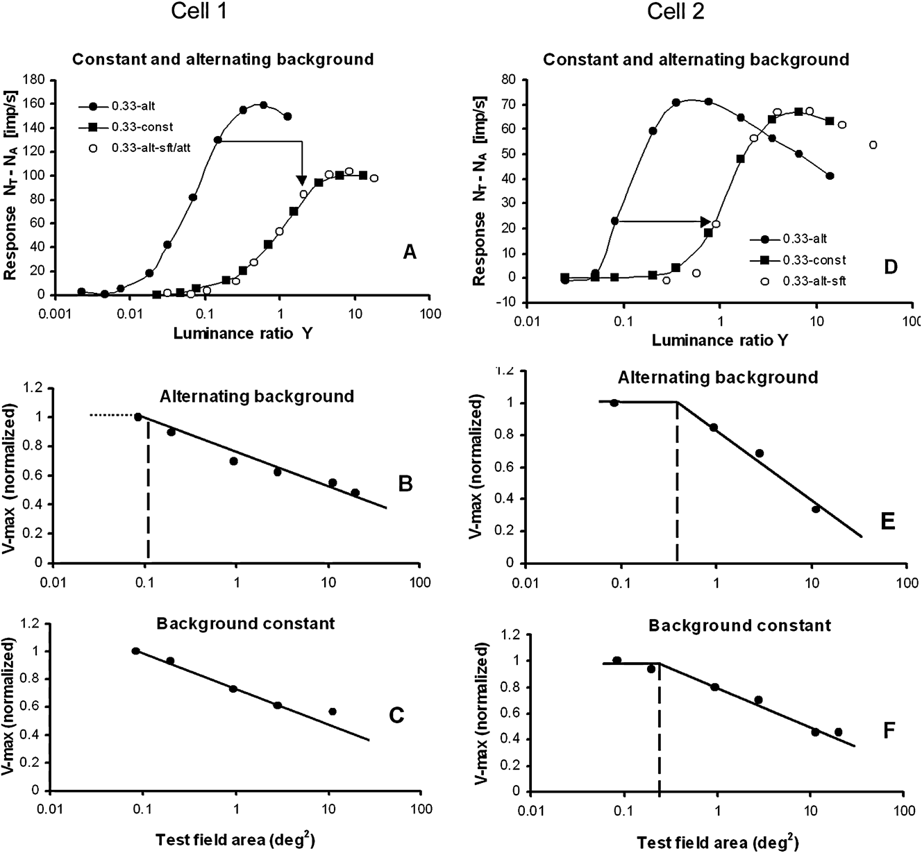
Responses plotted for stimuli presented upon a steady white background, or alternating with a white adapting background for two PC cells. (A) Cell 1: responses to a 0.33°-diameter test field for a “M–L” cell when the test and the background are alternating (filled circles) and when the background is constantly on (filled squares). Sensitivity is reduced (response curve is shifted to the right) and the responsiveness is attenuated by a constant factor when the background is steady (open circles). (B and C) For increasing test field sizes, the V max suppression in the surround closely follows a logarithmic function, both when the background is static (C) and when it is alternating (B). Cell: E10U07. “M–L” opponency. Eccentricity: 7°. (D) Cell 2: responses to a 0.33°-diameter test field for a “L–M” cell when the test and the background are alternating (filled circles) and when the background is constantly on (filled squares). The sensitivity is reduced (response curve shifted to the right), whereas the responsiveness is only slightly attenuated compared to the cell in Fig. 8A. (E and F) V max suppression in the surround follows a logarithmic function, both when the white background is static and when it is alternating. The center field becomes smaller when the background is constantly on. Cell: E20U02. Eccentricity: 5°.
The second example (displayed in Fig. 6B) shows how eqn. (1) can be used to predict prepotential activity when only the LGN response of a PC I-cell is recorded. The validity of the formula was verified by modeling the prepotentials for this “L–M” cell and demonstrated a close relationship with recordings (Seim et al., Reference Seim, Valberg and Lee2012, see their Fig. 7).
In a previous work (Lee et al., Reference Lee, Virsu and Creutzfeldt1983). it was shown that there is a close-to-linear relationship between LGN and prepotential responses when the color and luminance of a test field changed. That this is also the case for stimuli of different sizes is shown in Fig. 6C for a “L–M” cell.
Similar to the above findings for PC-cells, surround suppression was also found in the prepotentials of an MC cell suggesting that suppression is already present in the responses of retinal ganglion cells.
Discussion
Suppressive surround
The suppressive extraclassical surround is often represented by an extra Gaussian-shaped curve (Ghosh et al., Reference Ghosh, Sarkar and Bhaumik2005; Crook et al., Reference Crook, Manookin, Packer and Dacey2011) or as a network of small subunits (Bonin et al., Reference Bonin, Mante and Carandini2005; Solomon et al., Reference Solomon, Lee and Sun2006). In contrast, our experiments revealed a surround component, whose spatial sensitivity can be described by a power law. A comparison of a Gaussian- and a power-type spatial sensitivity of suppression is shown in Fig. 4L. The figure shows that for large test fields, the suppressive influence of the power function is much larger than that of the Gaussian function. For smaller test fields, the power function drops more quickly as a function of radius than does the Gaussian function. The constant (or absent) suppression in the center field is not predicted by the Gaussian function.
Suppression can be accounted for by a single spatial power sensitivity function with an exponent of ε = −1 in eqn. (6), derived from the surround response of PC cells (Fig. 4A and 4C), KC cells (Fig. 4E), and MC cells (Fig. 4G). Suppression, therefore, seems to be a common process that influences the responses of all three LGN cell types. Due to its multiplicative nature and large spatial extent, suppression is probably related to the extraclassical surround mechanism. In the work of Solomon et al. (Reference Solomon, White and Martin2002), on marmoset monkeys, it was found that suppression of the response to gratings was most prominent for MC cells and less so for PC cells and KC cells. In the work of Solomon et al. (Reference Solomon, Lee and Sun2006) on macaque monkeys with gratings, there were indications for suppressive surrounds for MC cells, but not for PC cells. In our experiment, using homogenous stimuli, surround suppression was found for all three cell types, but most prominent for MC cells.
Homogenous test fields vs. gratings and tiny spots
In the experiment presented here, the stimuli consisted of homogenous illuminated test fields of various sizes, with a luminance range of 3–6 log units and different spectral compositions. For these stimuli, the response behavior was not compatible with the results reported when nonhomogenous pattern stimuli were used, like gratings. Three response properties were incompatible with the DOG model: (a) the constant maximum response amplitude in the center of the receptive field. (b) The conservation of the excitatory/inhibitory balance for different stimulus sizes, found in both the center- and the surround field. (c) The suppression of maximum responsiveness with constant negative slope as a function of log area in the surround-field. For gratings, however, the contrast-enhancing DOG model largely describes a cell’s receptive field properties adequately (Hawken & Parker, Reference Hawken, Parker and Blakemore1990; Dacey et al., Reference Dacey, Packer, Diller, Brainard, Peterson and Lee2000; Cavanaugh et al., Reference Cavanaugh, Bair and Movshon2002; Solomon et al., Reference Solomon, White and Martin2002; McMahon et al., Reference McMahon, Packer and Dacey2004; Solomon et al., Reference Solomon, Lee and Sun2006; Alitto & Usrey, Reference Alitto and Usrey2008).
When a tiny test spot was placed in different positions within the center of the receptive field, then linear area summation of the responses was not observed. This was first shown by Kuffler (Reference Kuffler1953) and later, with better resolution, by Peichl and Wässle (Reference Peichl and Wässle1979) on X- and Y-ganglion cells in the cat retina. When a small spot of constant luminance, a size about one fifth of the receptive field center, is moved across the receptive field center, the response is progressively reduced when the spot is moved away from the center. This gives rise to a bell-shaped response curve, similar to a Gaussian curve. This is different from the response we get for centered, homogenous illuminated test fields of increasing size within the center field. Then the PC cell acts more like a light detector, similar to that used in a lux meter. When a small light spot, projected on the light-sensitive surface of the detector, is moved away from the center, the response is still constant, since the cell’s sensitivity is constant and independent of position within the light-sensitive surface. When the size of the spot is increased, the summation factor for the detector is 1.0. For a Gaussian-type sensitivity curve, with reduced sensitivity away from the center, the summation factor is less than 1.0 [predicted by Peichl and Wässle (Reference Peichl and Wässle1979) to be close to 0.8]. We predict that only when the central and the peripheral parts of the center field are illuminated simultaneously, there is area summation of sensitivity with a summation factor close to 1.
It is interesting to speculate if area summation within the center field is due to a retinal coincidence detector mechanism. A coincidence detector, generated by gap-junction activity of retinal amacrine cells (AII), has been found by Veruki & Hartveit (Reference Veruki and Hartveit2002). An alternative candidate might be the gap junctions between horizontal cells (Packer & Dacey, Reference Packer and Dacey2002).
The data shown in Fig. 6 strongly suggest that surround suppression also exists in retinal ganglion cells. A retinal origin is supported by Alitto & Usrey (Reference Alitto and Usrey2008) who pointed out that the extraclassical suppression in macaque LGN arises too quickly for being caused by cortical feedback. Others (Bonin et al., Reference Bonin, Mante and Carandini2005) have found that suppression in the retina is not significantly different from that in the LGN.
Since PC, KC, and MC cells in the LGN show the same kind of surround suppression, a possible candidate for the suppressive mechanism is retinal cells with lateral connections such as horizontal and amacrine cells. According to the work of McMahon et al. (Reference McMahon, Packer and Dacey2004) on macaques, the most probable candidate is the horizontal cells, since blocking the feedback from horizontal cells to cones leads to nearly complete disappearance of surround suppression. They also showed that amacrine cell activity only had a small influence upon the surround suppression.
Quantitative evaluation of model differences
Comparisons between the DOG model(s) and the responsivity and sensitivity derived from complete response curves are presented in Fig. 7. The spatial properties of the receptive fields of opponent LGN cells shown in Fig. 7A are difficult to detect when more traditional methods are used, like a threshold- or a sensitivity criterion, where sensitivity is equal to 1/threshold luminance. In Fig. 7A, a threshold criterion of 5 imp/s is shown by the horizontal dashed line. When using this threshold method, only the excitatory component of an opponent cell is analyzed since the inhibitory mechanism is not yet activated. The close to constant responsiveness of the cell in the center field is not revealed by this method.
In Fig. 7A, we also see that the steepness of the slope (the gain) of the response at low intensities is reduced as suppression increases for large test fields. The gain and the responsiveness are related concepts, and gain changes influence both the excitatory and the inhibitory components.
Also in another method, using a constant luminance ratio for the stimulus (as indicated by the vertical dashed line in Fig. 7A), mainly the excitatory response component is measured. In such experiments, it is customary to use the maximum response as criterion for the size of the receptive field center (Ruksenas et al., Reference Ruksenas, Fjeld and Heggelund2000). From Fig. 7A, we see that this is correct since maximum response is obtained for the gray curve, representing the limiting size of the center field. This method leads to the same size of the center field as that shown in Figs. 4A, 4C, and 7B.
In Fig. 7B, the maximum responsiveness of a DOG model (thick curve) is compared with that obtained from the model in Fig. 7A (open circles). The low responsiveness of the DOG model, seen for small test spots, is not found in our experiment. Instead, the responsiveness was high and constant within the center area. The logarithmic attenuation for larger test fields continued until the response was totally abolished, contrary to the DOG model where the responsiveness did not change for the larger areas. The size of the center field, derived from grating stimuli and by using the DOG model, is smaller than the summation center found with homogenous illuminated stimuli. The responses shown in Fig. 7A and 7B are mathematically represented by eqn. (7A). When the coefficients a and b are known from the experiment, the area φ of the center field can be found from the equation log(φ) = (1 − b)/a.
In Fig. 7C, the sensitivity of the LGN cell is calculated by the DOG models and by the model applied in Fig. 7A. For small homogenous test fields of increasing size, the slope k of the sensitivity within the center field is close to 1, as found by Peichl and Wässle (Reference Peichl and Wässle1979) and by Crook et al. (Reference Crook, Lange-Malecki, Lee and Valberg1988) for spot sizes as small as 0.05° diameter (area 0.008 deg2). In eqn. (7C), a slope of 1.0 is obtained when d = 1.0. The constant sensitivity, seen for test fields larger than the center field, is obtained when the value of c in eqn. (7C) is constant.
Except for very small spots, the slope of the DOG models is less than 1.0, and it decreases gradually when spot sizes increases, until maximum sensitivity is reached. Moreover, Peichl and Wässle noted that for a DOG type I model (Fig. 1A), the threshold luminance should rise significantly and reduce the sensitivity when the spot size was made larger than the center field, as indicated by the thick DOG-labeled curve in Fig. 7C. This was due to the increased strength of the inhibitory surround component in Fig. 1A. However, this was not found in their experiment. Instead, a close-to-constant threshold response was found for test spots larger than the center field.
In a DOG type II model, the spatial size of excitatory and inhibitory Gaussian functions have identical spatial extent, because α L = α M in eqn. (3). For a DOG type II model, the slope of the sensitivity curve for small test fields deviates from 1.0 in a similar way as seen for the DOG type I. For large test fields, the response for this model becomes constant.
In Fig. 7D, the ratio between the excitatory and inhibitory components of an opponent cell is plotted as a function of test field size for the DOG model. From eqn. (4), this ratio is expressed as  $g(r,L) * {V_{\rm{L}}}/g(r,M) * {V_{\rm{M}}}$. For the DOG model, this ratio changes considerably when the test field size increases. This represents a serious problem for color perception, since it would mean that a color of the same chromaticity changes significantly with area (see under Color appearance below). For the new model of an “L–M” cell presented in Fig. 7A and eqn. (1B), the excitatory/inhibitory ratio,
 ${A_{\rm{L}}} * {V_{\rm{L}}}/{A_{\rm{M}}} * {V_{\rm{M}}}$, is constant for all spot sizes.
Center size variability
The size of the receptive field center for homogenous illuminated stimuli is dependent on stimulus configurations. As exemplified in Fig. 7C, the largest centers are obtained for excitatory wavelengths. The size of the center, when recorded with a steady background, was slightly smaller than when using an alternating background, as shown by the response labeled Constant BG. When the excitatory test stimulus was replaced by an achromatic stimulus, the center field area (where linear summing takes place) is significantly reduced (see response-labeled Achromatic color). This indicates that the size of the center field depends on stimulus color and the state of adaptation.
The size of the center field was strongly increased when an achromatic test field was replaced by an excitatory color stimulus, as shown in Fig. 4K. But for the grating experiments, the resolution increased when an achromatic stimulus was replaced with an excitatory color (Crook et al., Reference Crook, Lange-Malecki, Lee and Valberg1988). Smaller center fields are associated with increased resolution, and this suggests therefore that the contrast-sensitive mechanism acts in an opposite way of what is found for homogenous stimuli. For homogenous stimuli, the size of the receptive field center is significantly larger than what is expected from dendritic connections of cone, bipolar, and ganglion cells, as found for cells at relevant retinal eccentricities (Dacey et al., Reference Dacey, Packer, Diller, Brainard, Peterson and Lee2000; Crook et al., Reference Crook, Manookin, Packer and Dacey2011). Einevoll et al. (Reference Einevoll, Jurkus and Heggelund2011) have shown that temporal changes also influence the size of summation of receptive field center areas. This variability in size may indicate that size is influenced by lateral mechanism(s) in the retina that behave differently to different types of stimulation.
In our experiments, the receptive field center of PC cells (as determined in Fig. 4A and 4B) varied approximately from 0.3 to 1° diameter for excitatory colors (the average size of the center was not available because six cells had center sizes smaller than the smallest test spot used). But for achromatic or neutral (571 nm) colors, the center field becomes smaller than the smallest test spots used, as shown in Fig. 4K. The size of the center field for achromatic colors might be deduced from results obtained from the macaque retina (Crook et al., Reference Crook, Lange-Malecki, Lee and Valberg1988). They found that the center diameter averaged around 0.15° diameter for eccentricities between 6 and 14°. However, in their experiments, the test field was presented upon a steady background, a condition for which the center sizes were found to be reduced (see Appendix).
Our commonly used test fields larger than 0.3° might explain the missing center response for MC cells in Fig. 4H. Crook et al. (Reference Crook, Lange-Malecki, Lee and Valberg1988), using the threshold method for defining the size of the center, got MC cell sensitivity slopes close to 1.0. The center sizes varied from approximately 0.12 to 0.4° diameter, with an average around 0.2°. The reason for the missing center break seen in Fig. 4H for all except one MC cell is probably due to the use of too large test fields.
Color appearance
Color vision is a suprathreshold photopic phenomenon, reflecting the relative activities of cones and their combinations in different types of cone-opponent cells. Under normal daylight conditions, the contrast range of visual stimuli covers several log units; yet most neurophysiological studies of color vision have dealt with the threshold sensitivity of opponent cells. Such studies have provided valuable insight into the mechanisms of color detection and discrimination but fail to account for nonlinear suprathreshold attributes and their scaling in familiar color systems.
In order to make object color appearance close to independent of stimulus size, it is essential that excitatory and inhibitory cone inputs to opponent cells balance each other. In the experiment presented here, this balance is found for all test field sizes for the majority of the opponent LGN cells, in agreement with a power-law behavior of the dependence of both excitation and inhibition on stimulus size. This balance is contrary to the prediction of the DOG model, for which the balance changes continuously when the size of the test field changes (Fig. 7D).
Adaptation
In the macaque, the adaptive effect of a stationary white annulus, placed in the ECRF, is well known (Valberg et al., Reference Valberg, Lee, Tigwell and Creutzfeldt1985). It causes a shift of spectral I–R curves of PC-cells toward higher luminance ratios. A similar result has been reported by Benardete and Kaplan (Reference Benardete and Kaplan1999). The strength of adaptation varied with the radius and luminance of the annulus.
When a small test spot is presented for 300 ms in the receptive field center and an annulus is presented simultaneously in the ECRF, then the response of the test spot is attenuated (Valberg et al., Reference Valberg, Lee, Tigwell and Creutzfeldt1985). The attenuation increases with the luminance and the area of the annulus, the effect of the annulus being equivalent to adaptation.
The test stimulus itself, lasting for only 300 ms, may also transiently adapt the cell, and more so for high-luminance test fields, with sizes well into the ECRF and presented on a steady background. But what will be the adaptive effect of smaller less intense test fields? There might be a lower limit, below which the size of the stimulus field does not affect the adaptive mechanism. Our main finding, that when the size of small test stimuli increased beyond a given value (i.e., the size of the center field), the cell’s responsivity decreased, might be interpreted as adaptation. The larger the test field, the stronger the adaptation. Since the test field is presented only for 300 ms, the adaptation may be in a transient phase, leading to a decrease in responsivity but not yet influencing the sensitivity of the response.
Conclusion
For stimuli with spatial contrast, like gratings, the DOG model successfully predicts linear responses. However, this model fails to describe the balance needed between excitatory and inhibitory processes (opponency) in order to maintain color (hue) stability for stimuli of different sizes but with the same CIE chromaticity and luminance factor. On the other hand, homogeneous stimuli, like the ones used here, do not appear to activate the contrast-sensitive mechanisms. Instead, these stimuli activate visual mechanisms that are responsible for color stability and adaptation. Characteristic of these responses are the constant responsiveness in the center of the receptive field and surround suppression expressed by a power function.
Acknowledgment
This work was supported in part by a grant from the International Neuroinformatics Coordinating Facility (incf) to AV and NEI EY13112 grant to BBL. We thank Barry B. Lee and Jan Kremers for their help in collecting these data and for helpful discussions, and Paul Heggelund and Espen Hartveit for valuable comments on the manuscript.
Appendix Alternating contra steady backgrounds
In order to rule out the possibility that the main experimental results, and the power law deduced from them, have unduly been influenced by the stimulus configuration, as when the large (4 × 5 deg2) adapting field is turned off and a small test stimulus is presented for a short time on a dark background. By using a dark background, the test stimulus was pure and not affected in any way by additive color mixture of stimulus and adapting field, contrary to using a steady white background that influences adaptation, and where the colorimetric purity of the stimulus is substantially reduced. In order to check for a possible difference, 26 Increment cells were measured while the adapting field was steadily present. For six cells, stimuli of varying sizes were used, together with both an alternating and a constant background.
In Fig. 8A–8C and 8D–8F, the response for two PC cells to a small (0.33°) spot is plotted for alternating and steady backgrounds. For both cells (Fig. 8A and 8D), the resulting response curve for the steady background was shifted approximately 1.1 log units to the right on the x-axis relative to the alternating background. In addition, for the cell in Fig. 8A, the responsivity was attenuated by a factor of 0.65, whereas the cell in Fig. 8D was only slightly attenuated. After shifting and attenuating the response curve for the alternating background, the modified response closely followed that obtained for a constant white background. A similar sensitivity shift was found for most of the 26 cells.
Six test spot sizes were used for the cell in Fig. 8A, and for all sizes, the response curves for the alternating background had to be shifted 1.15 log units and attenuated by a factor of 0.65 to fit the response curves with a steady background. For this cell, the strength of the surround suppression was similar for both stimulus situations (Fig. 8B and 8C), although it varied for the other cell. The figures show that the center field was usually found to be smaller when the background was steady.
These results demonstrate that a common curve, shifted and/or attenuated, could describe the results when the background was steady. Similar to the experiment with alternating background, the surround suppression with a steady background could be accounted for by a logarithmic function of the test spot area.