1 Introduction
Swimming organisms self-propel with hydrodynamic footprints that are unique to their species. Their hydrodynamic footprints eventually dissipate because of the viscosity of the fluid. The perturbed flows that persist before complete dissipation affect the movements of the surrounding organisms. Such perturbed flows arise due to both stationary objects and other moving organisms (e.g. birds flocking, fish schooling). The flow-mediated interactions between organisms and stationary objects are unidirectional, whereas the interactions between moving organisms are bidirectional. Hydrodynamic research has demonstrated that the perturbed flow formed from a stationary object is somewhat controllable, which has enabled the elucidation of the mechanisms underlying the hydrodynamic interactions with surrounding organisms (Liao et al. Reference Liao, Beal, Lauder and Triantafyllou2003a ,Reference Liao, Beal, Lauder and Triantafyllou b ; Ulrike Reference Ulrike2003; Liao Reference Liao2004, Reference Liao2007; Beal et al. Reference Beal, Hover, Triantafyllou, Liao and Lauder2006; Eldredge & Pisani Reference Eldredge and Pisani2008; Park, Kim & Sung Reference Park, Kim and Sung2016). On the other hand, investigating the perturbed flows produced by other moving organisms is tricky: the flow complexity increases as the population of organisms increases, which makes the analysis of the hydrodynamic interactions difficult.
Multi-party flow-mediated interaction has been widely observed in swimming fish. The inviscid theoretical model of Weihs (Reference Weihs1973) demonstrated that trailing fish in a diamond configuration can benefit from the reduced flow induced by the oncoming vortices. According to the experimental studies performed by Herskin & Steffensen (Reference Herskin and Steffensen1998) and Svendsen et al. (Reference Svendsen, Skov, Bildsoe and Steffensen2003), trailing fish reduced their tail beats while maintaining the same speed as that of the leading fish. Fish with a high aerobic capacity had a tendency to swim in the front part of schools and overcame an increased drag, while fish with a low maximal metabolic rate were located in the rear part and reduced tail beats (Killen et al. Reference Killen, Marras, Steffensen and Mckenzie2012). Marras et al. (Reference Marras, Killen, Lindstrom, McKenzie, Steffensen and Domenici2015) found that both upstream and downstream fish saved energy regardless of their positions. Although many recent experimental studies have shown the hydrodynamic benefits of fish schools (Herskin & Steffensen Reference Herskin and Steffensen1998; Svendsen et al. Reference Svendsen, Skov, Bildsoe and Steffensen2003; Killen et al. Reference Killen, Marras, Steffensen and Mckenzie2012; Marras et al. Reference Marras, Killen, Lindstrom, McKenzie, Steffensen and Domenici2015), the question of which schooling structures are optimal from a hydrodynamic point of view is still controversial, and an in-depth understanding of the hydrodynamic mechanisms by which fish schools benefit from flow-mediated interactions is desirable.
Computational simulations have helped shed light on the hydrodynamic mechanisms of fish schooling by modelling schools as travelling wavy foils (Deng & Shao Reference Deng and Shao2006; Deng, Shao & Yu Reference Deng, Shao and Yu2007; Dong & Lu Reference Dong and Lu2007; Gazzola et al. Reference Gazzola, Chatelain, Ress and Koumoustsakos2011; Gazzola, Hejazialhosseini & Koumoutsakos Reference Gazzola, Hejazialhosseini and Koumoutsakos2014b ; Daghooghi & Borazjani Reference Daghooghi and Borazjani2015; Hemelrijk et al. Reference Hemelrijk, Reid, Hildenbrandt and Paddling2015; Tian et al. Reference Tian, Wang, Wu and Sui2016; Lin et al. Reference Lin, He, He, Wang and Chen2017; Maertens, Gao & Triantafyllou Reference Maertens, Gao and Triantafyllou2017; Novati et al. Reference Novati, Verma, Alexeev, Rossinelli, Rees and Koumoutsakos2017), multiple finite dipoles (Tchieu, Kanso & Newton Reference Tchieu, Kanso and Newton2012; Tsang & Kanso Reference Tsang and Kanso2013; Gazzola et al. Reference Gazzola, Tchieu, Alexeev, Brauer and Koumoutsakos2016), or multiple flexible filaments (Zhu & Peskin Reference Zhu and Peskin2003; Huang, Shin & Sung Reference Huang, Shin and Sung2007; Alben Reference Alben2009; Zhu Reference Zhu2009; Kim, Huang & Sung Reference Kim, Huang and Sung2010; Uddin, Huang & Sung Reference Uddin, Huang and Sung2013; Zhu, He & Zhang Reference Zhu, He and Zhang2014a ; Uddin, Huang & Sung Reference Uddin, Huang and Sung2015; Son & Lee Reference Son and Lee2017). For two travelling wavy foils in a tandem configuration, the downstream fish saved energy at any position by appropriately modulating its body motions according to the oncoming vortices shed from the upstream fish (Maertens et al. Reference Maertens, Gao and Triantafyllou2017). The upstream fish benefited only for a small streamwise gap distance (Deng et al. Reference Deng, Shao and Yu2007; Maertens et al. Reference Maertens, Gao and Triantafyllou2017). The hydrodynamic advantages were attainable in a diagonal schooling configuration (Tian et al. Reference Tian, Wang, Wu and Sui2016; Lin et al. Reference Lin, He, He, Wang and Chen2017) and the efficiency of the downstream fish was increased by up to 80 % by reducing the flapping amplitude (Maertens et al. Reference Maertens, Gao and Triantafyllou2017). The trailing fish in an inverted triangular configuration can save energy in a reverse Kármán vortex street (Deng & Shao Reference Deng and Shao2006). Infinite fish schools of in-line, side-by-side, diamond (Hemelrijk et al. Reference Hemelrijk, Reid, Hildenbrandt and Paddling2015) and rectangular configurations (Daghooghi & Borazjani Reference Daghooghi and Borazjani2015) were modelled by using periodic boundary conditions, and demonstrated global energy savings for such schools. Although the use of travelling wavy foils enabled the realistic modelling of fish-like body shapes and motions, the schooling structures were pre-specified rather than dynamically determined. The swimmers modelled in Gazzola et al. (Reference Gazzola, Hejazialhosseini and Koumoutsakos2014b ) and Novati et al. (Reference Novati, Verma, Alexeev, Rossinelli, Rees and Koumoutsakos2017) adjusted their swimming motions and relative positions to reach a specified goal by employing reinforcement learning. Two swimmers could not self-sustain their tandem configuration with a priori specified flapping motion (Novati et al. Reference Novati, Verma, Alexeev, Rossinelli, Rees and Koumoutsakos2017). The follower adjusted its swimming kinematics and maintained a stable tandem configuration through reinforcement learning, where the energy expenditure was reduced by up to 30 % for the follower (Novati et al. Reference Novati, Verma, Alexeev, Rossinelli, Rees and Koumoutsakos2017).
Tchieu et al. (Reference Tchieu, Kanso and Newton2012) modelled multiple finite dipoles in an unbounded fluid to investigate the far-field hydrodynamics in fish schools. The dipole system was considered as a group of swimmers which interacted among themselves dynamically. Tsang & Kanso (Reference Tsang and Kanso2013) used the model in a doubly periodic domain and examined two types of dipole lattices: rectangular and diamond. The linear stability of the two dipole lattices showed that the rectangular dipole lattice was unstable and required active stabilization, while the diamond lattice was passively stable to small perturbations (Tsang & Kanso Reference Tsang and Kanso2013). Gazzola et al. (Reference Gazzola, Tchieu, Alexeev, Brauer and Koumoutsakos2016) adopted a reinforcement learning algorithm for adaptive group swimming, where multiple finite dipoles adjusted their speed and orientation according to varying hydrodynamic loads. A schooling pattern of ‘hourglass’-shape was identified as exhibiting minimal collective effort.
The hydrodynamic mechanisms by which fish exploit energy from surrounding unsteady flows through self-adjusting flapping motions are based on fluid–flexible-body interactions. Fish swimming through a Kármán vortex street formed by a D-section cylinder immersed in a uniform flow activated only their anterior muscles, with other posterior parts fluttered passively as a result of fluid–flexible-body interactions (Liao et al. Reference Liao, Beal, Lauder and Triantafyllou2003a ; Liao Reference Liao2004). The flexible characteristics of swimmers, which were not considered in the travelling wavy foil or vortex dipole model, can be treated by adopting a flexible filament subjected to oncoming flows. Zhu & Peskin (Reference Zhu and Peskin2003) and Huang et al. (Reference Huang, Shin and Sung2007) analysed the interactions between two side-by-side flexible filaments tethered on their leading edges. The spanwise gap distance was one of the key factors in determining the in-phase and out-of-phase flapping motions between the two filaments. In a fixed tandem configuration, the drag force on the downstream flag decreased or increased when destructive or constructive vortex interaction modes occurred, respectively, which depended on the streamwise gap distance (Alben Reference Alben2009; Kim et al. Reference Kim, Huang and Sung2010). Triangular, diamond and conical configurations of multiple flexible flags with predetermined relative positions were modelled, and the flags fluttered passively interacting with the surrounding fluid (Uddin et al. Reference Uddin, Huang and Sung2013). The tethered systems did not take into account the dynamic nature of fish schooling since the individuals within a school could not change their relative positions in response to the surrounding fluid. Two flexible filaments propelled in a tandem configuration changed the relative position and formed stable configurations by locking onto the oncoming vortex centres, where the input power of the downstream filament was reduced (Zhu et al. Reference Zhu, He and Zhang2014a ).
The goals of the present study were to find a stable configuration of the flexible fins and to optimize the propulsive efficiency by reducing the heaving amplitude of the trailing fins while keeping a stable configuration. The present study, motivated by the work of Weihs (Reference Weihs1973), mainly explored the dynamics of flexible fins propelled in a diamond configuration, which consists of tandem, diagonal and triangular configurations. Although fish schools with various configurations have been extensively studied, the introduction of dynamic considerations into the study of fish schooling results in more complicated flow-mediated interactions between individuals. Our results for flexible fins propelled in various configurations with relative positions that change dynamically in the horizontal direction are expected to provide a better understanding of fish schooling. We examined whether stable configurations can form spontaneously through vortex–vortex and vortex–flexible-body interactions alone, and determined the energetic benefits for individuals of varying their local positions. Section 2 introduces the problem formulation and describes the numerical method. Our numerical results are presented and discussed in § 3. Conclusions are drawn in § 4.
2 Problem formulation
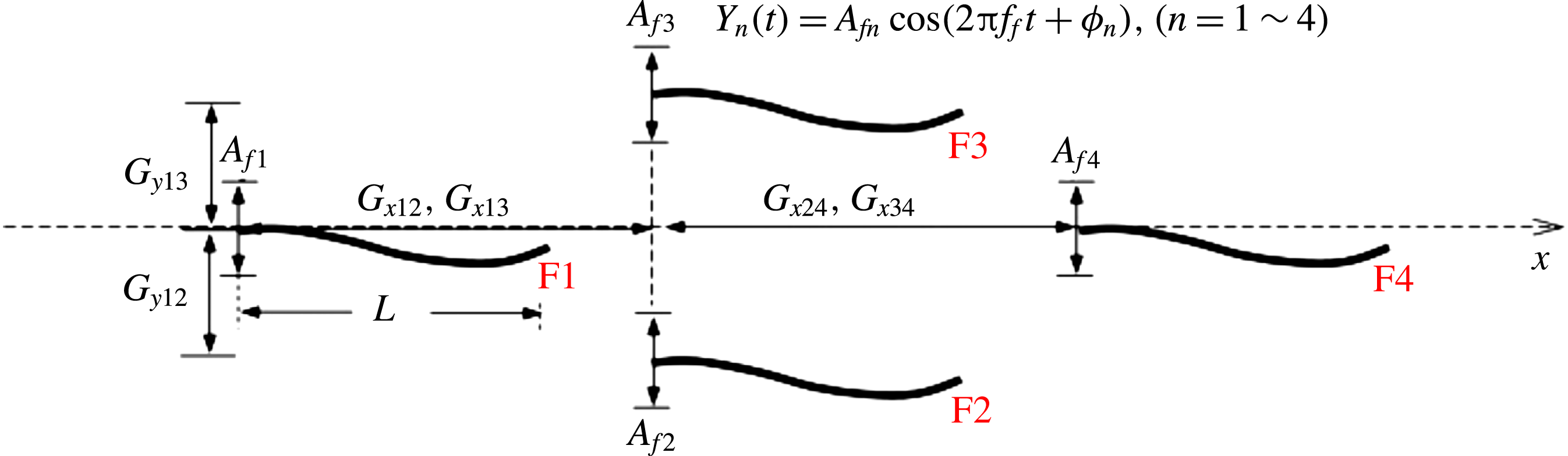
A two-dimensional simulation was performed for groups of two, three, or four flexible fins propelled in tandem, diagonal, triangular, or diamond configurations. Figure 1 shows a schematic diagram of the coordinate system and the diamond configuration, where Fin 1 (F1) and Fin 4 (F4) are the leading and trailing fins, respectively, and Fin 2 (F2) and Fin 3 (F3) are positioned in the middle row. A transverse heaving motion characterized by a heaving amplitude
 $A_{f}$
and a frequency
 $f_{f}$
was prescribed on the leading edge of each fin under a clamped boundary condition. A free-end boundary condition was imposed on the trailing edge of each fin. The flexible fins were not constrained horizontally, but constrained transversely due to the imposed heaving motion on their leading edges. A rotating motion was not allowed for the flexible fins. The relative positions of the four flexible fins can be specified regarding the streamwise gap distance
 $G_{x}$
and the spanwise gap distance
 $G_{y}$
; the subscripts are the fin numbers, i.e.
 $G_{x12}$
is the streamwise gap distance between F1 and F2. The flexible fins spontaneously change their relative positions in the horizontal direction as a result of the fluid–flexible-body interactions, and the schooling structure is dynamically determined. The fluid domain was defined by a fixed Eulerian coordinate system, and a moving Lagrangian coordinate system was applied to each flexible fin. The motions of the fluid and flexible fins were independently solved in each grid system and then coupled by using the immersed boundary (IB) method (Huang et al.
Reference Huang, Shin and Sung2007).
Schematic diagram of four flexible fins propelled in a diamond configuration.

The fluid motion was governed by the incompressible Navier–Stokes equations, which were non-dimensionalized by introducing the following characteristic scales: the maximum flapping velocity of the heaving motion
 $U_{ref}$
(
 $=2\unicode[STIX]{x03C0}A_{f1}f_{f1}$
) for the velocity
 $\boldsymbol{u}$
, the fin body length
 $L$
for the length, the fluid density
 $\unicode[STIX]{x1D70C}_{0}$
for the density,
 $L/U_{ref}$
for the time
 $t$
,
 $\unicode[STIX]{x1D70C}_{0}U_{ref}^{2}$
for the pressure
 $p$
and
 $\unicode[STIX]{x1D70C}_{0}U_{ref}^{2}/L$
for the momentum forcing
 $\boldsymbol{f}$
. The reference velocity
 $U_{ref}$
was fixed to 1. The non-dimensional Navier–Stokes and continuity equations are
 $$\begin{eqnarray}\displaystyle & \displaystyle \frac{\unicode[STIX]{x2202}\boldsymbol{u}}{\unicode[STIX]{x2202}t}+\boldsymbol{u}\boldsymbol{\cdot }\unicode[STIX]{x1D735}\boldsymbol{u}=-\unicode[STIX]{x1D735}p+\frac{1}{Re}\unicode[STIX]{x1D6FB}^{2}\boldsymbol{u}+\boldsymbol{f}, & \displaystyle\end{eqnarray}$$
 $$\begin{eqnarray}\displaystyle & \displaystyle \unicode[STIX]{x1D735}\boldsymbol{\cdot }\boldsymbol{u}=0, & \displaystyle\end{eqnarray}$$
where Re is the flapping Reynolds number,
 $Re=\unicode[STIX]{x1D70C}_{0}U_{ref}L/\unicode[STIX]{x1D707}$
, and
 $\unicode[STIX]{x1D707}$
is the dynamic viscosity. The motions of the flexible fins were governed by the nonlinear structural equation under the inextensibility condition, which was non-dimensionalized with the following characteristic scales:
 $\unicode[STIX]{x1D70C}_{1}U_{ref}^{2}$
for the tension force
 $T$
,
 $\unicode[STIX]{x1D70C}_{1}U_{ref}^{2}L^{2}$
for the bending rigidity
 $\unicode[STIX]{x1D6FE}$
and
 $\unicode[STIX]{x1D70C}_{1}U_{ref}^{2}/L$
for the Lagrangian momentum force
 $\boldsymbol{F}$
, which is the counterpart of
 $\boldsymbol{f}$
in (2.1).
 $\unicode[STIX]{x1D70C}_{1}$
is the density difference between the fin and the surrounding fluid (Uhlmann Reference Uhlmann2005; Yu Reference Yu2005) and set to 1 in the present simulation. The non-dimensional fin motion equation is given by
 $$\begin{eqnarray}\displaystyle & \displaystyle \frac{\unicode[STIX]{x2202}^{2}\boldsymbol{X}}{\unicode[STIX]{x2202}t^{2}}=\frac{\unicode[STIX]{x2202}}{\unicode[STIX]{x2202}s}\left(T\frac{\unicode[STIX]{x2202}\boldsymbol{X}}{\unicode[STIX]{x2202}s}\right)-\frac{\unicode[STIX]{x2202}^{2}}{\unicode[STIX]{x2202}s^{2}}\left(\unicode[STIX]{x1D6FE}\frac{\unicode[STIX]{x2202}^{2}\boldsymbol{X}}{\unicode[STIX]{x2202}s^{2}}\right)-\boldsymbol{F}, & \displaystyle\end{eqnarray}$$
 $$\begin{eqnarray}\displaystyle & \displaystyle \frac{\unicode[STIX]{x2202}\boldsymbol{X}}{\unicode[STIX]{x2202}s}\boldsymbol{\cdot }\frac{\unicode[STIX]{x2202}\boldsymbol{X}}{\unicode[STIX]{x2202}s}=1, & \displaystyle\end{eqnarray}$$
where
 $s$
is the Lagrangian variable and
 $\boldsymbol{X}=(X(s,t),Y(s,t))$
is the position vector. Since the fin motion equation is one-dimensional in space, the actual line density of the fin is
 $\unicode[STIX]{x1D70C}_{1}+\unicode[STIX]{x1D70C}_{0}A$
, where
 $A$
is the sectional area of the fin. The bending rigidity
 $\unicode[STIX]{x1D6FE}$
was set to 1 and the tension force
 $T$
is a function of the Lagrangian variable
 $s$
and the time
 $t$
. The tension force was determined from the inextensibility constraint and calculated by solving the Poisson equation derived from (2.3) and (2.4):
 $$\begin{eqnarray}\displaystyle \displaystyle \frac{\unicode[STIX]{x2202}\boldsymbol{X}}{\unicode[STIX]{x2202}s}\boldsymbol{\cdot }\frac{\unicode[STIX]{x2202}^{2}}{\unicode[STIX]{x2202}s^{2}}\left(T\frac{\unicode[STIX]{x2202}\boldsymbol{X}}{\unicode[STIX]{x2202}s}\right) & = & \displaystyle \frac{1}{2}\frac{\unicode[STIX]{x2202}^{2}}{\unicode[STIX]{x2202}t^{2}}\left(\frac{\unicode[STIX]{x2202}\boldsymbol{X}}{\unicode[STIX]{x2202}s}\boldsymbol{\cdot }\frac{\unicode[STIX]{x2202}\boldsymbol{X}}{\unicode[STIX]{x2202}s}\right)-\frac{\unicode[STIX]{x2202}^{2}\boldsymbol{X}}{\unicode[STIX]{x2202}t\unicode[STIX]{x2202}s}\boldsymbol{\cdot }\frac{\unicode[STIX]{x2202}^{2}\boldsymbol{X}}{\unicode[STIX]{x2202}t\unicode[STIX]{x2202}s}\nonumber\\ \displaystyle & & \displaystyle +\,\frac{\unicode[STIX]{x2202}\boldsymbol{X}}{\unicode[STIX]{x2202}s}\boldsymbol{\cdot }\frac{\unicode[STIX]{x2202}}{\unicode[STIX]{x2202}s}\left(\frac{\unicode[STIX]{x2202}^{2}}{\unicode[STIX]{x2202}s^{2}}\left(\unicode[STIX]{x1D6FE}\frac{\unicode[STIX]{x2202}^{2}\boldsymbol{X}}{\unicode[STIX]{x2202}s^{2}}\right)+\boldsymbol{F}_{\boldsymbol{l}}\right).\end{eqnarray}$$
The boundary conditions applied to the leading and trailing edges were
 $$\begin{eqnarray}\displaystyle & \displaystyle Y(t)=\frac{A_{f}}{2}\cos (2\unicode[STIX]{x03C0}\,f_{f}t+\unicode[STIX]{x1D711}),\quad \frac{\unicode[STIX]{x2202}\boldsymbol{X}}{\unicode[STIX]{x2202}s}=(1,0),\quad \frac{\unicode[STIX]{x2202}^{3}X}{\unicode[STIX]{x2202}s^{3}}=0\quad \text{at }s=0, & \displaystyle\end{eqnarray}$$
 $$\begin{eqnarray}\displaystyle & \displaystyle T=0,\quad \frac{\unicode[STIX]{x2202}^{2}\boldsymbol{X}}{\unicode[STIX]{x2202}s^{2}}=(0,0),\quad \frac{\unicode[STIX]{x2202}^{3}\boldsymbol{X}}{\unicode[STIX]{x2202}s^{3}}=(0,0)\quad \text{at }s=1. & \displaystyle\end{eqnarray}$$
The boundary condition in (2.6) imposed on the leading edge combines the transverse harmonic heaving motion, the clamped condition and the horizontally unconstrained condition. The free-end boundary condition in (2.7) was applied at the trailing edge.
The interaction force between the fluid and the fin was calculated with a feedback force law and the Lagrangian momentum force
 $\boldsymbol{F}$
was obtained from the equation
 $$\begin{eqnarray}\displaystyle & \displaystyle \boldsymbol{F}(s,t)=-\unicode[STIX]{x1D705}\left[\left(\boldsymbol{X}_{ib}-\boldsymbol{X}\right)+\unicode[STIX]{x0394}t\left(\boldsymbol{U}_{ib}-\boldsymbol{U}\right)\right], & \displaystyle\end{eqnarray}$$
where
 $\unicode[STIX]{x1D705}=-2\times 10^{6}$
is a user-defined constant,
 $\unicode[STIX]{x0394}t$
denotes the computational time step and
 $\boldsymbol{U}$
is the velocity of the fin expressed by
 $\boldsymbol{U}=\text{d}\boldsymbol{X}/\text{d}t$
. The Lagrangian momentum force was little affected by varying the user-defined constant by the feedback force law once
 $\unicode[STIX]{x1D705}$
was given by the value within the stability regime reported in Shin, Huang & Sung (Reference Shin, Huang and Sung2008). The subscript ‘ib’ in (2.8) denotes the variables of the immersed boundary (IB) points, which moved with the ambient fluids. The velocity of the IB (
 $\boldsymbol{U}_{ib}$
) was determined by the fluid velocity interpolated at the IB and calculated by
 $$\begin{eqnarray}\displaystyle & \displaystyle \boldsymbol{U}_{ib}(s,t)=\int _{\unicode[STIX]{x1D6FA}}\boldsymbol{u}(\boldsymbol{x},t)\unicode[STIX]{x1D6FF}(\boldsymbol{X}(s,t)-x)\,\text{d}x, & \displaystyle\end{eqnarray}$$
where the transformation between the Eulerian and Lagrangian variables was realized by using the smoothed Dirac delta function (Peskin Reference Peskin2002). The position of the IB (
 $\boldsymbol{X}_{ib}$
) was derived by
 $$\begin{eqnarray}\displaystyle & \displaystyle \boldsymbol{X}_{ib}=\boldsymbol{X}_{ib}^{0}+\int _{0}^{t}\boldsymbol{U}_{ib}\,\text{d}t, & \displaystyle\end{eqnarray}$$
where
 $\boldsymbol{X}_{ib}^{0}$
is the initial position of the IB. The Eulerian momentum force
 $\boldsymbol{f}$
was calculated by spreading the Lagrangian force
 $\boldsymbol{F}$
to the nearby Eulerian grid points with the smoothed Dirac delta function,
 $$\begin{eqnarray}\displaystyle & \displaystyle \boldsymbol{f}(x,t)=\frac{\unicode[STIX]{x1D70C}_{1}}{\unicode[STIX]{x1D70C}_{0}L}\int _{\unicode[STIX]{x1D6E4}}\boldsymbol{F}(s,t)\unicode[STIX]{x1D6FF}(\boldsymbol{x}-\boldsymbol{X}(s,t))\,\text{d}s, & \displaystyle\end{eqnarray}$$
where
 $\unicode[STIX]{x1D70C}_{1}/\unicode[STIX]{x1D70C}_{0}L$
is derived from the non-dimensionalization process. The combination of (2.8)–(2.11) indicated that the velocities at the ambient Eulerian grids moved with those of the Lagrangian grids, enforcing the no-slip boundary condition of the fluid on the fin.
For numerical implementation, the fluid governing equations (2.1) and (2.2) were solved by using the fractional step method on a staggered Cartesian grid system, and second-order accuracy was guaranteed in time for velocity and pressure (Kim, Baek & Sung Reference Kim, Baek and Sung2002). The finite difference method was used to solve the fin motion equations (2.3) and (2.4). More details of the numerical schemes are described in Huang et al. (Reference Huang, Shin and Sung2007), Huang & Sung (Reference Huang and Sung2010). The overall numerical procedure for simulating the flexible fins arranged in the four basic configurations can be summarized as follows:
-
(1) At the
 $n$
th time step, the fluid velocity
$\boldsymbol{u}^{n}$
and the fin positions
$\boldsymbol{X}^{n}$
and
$\boldsymbol{X}^{n-1}$
are known.
$\boldsymbol{U}_{ib}^{n}$
is calculated by interpolating the fluid velocity at the IB in (2.9).
-
(2) The Lagrangian interaction force
$\boldsymbol{F}^{n}$
is obtained in (2.8). -
(3) The Eulerian interaction force
$\boldsymbol{f}^{n}$
is calculated by spreading the Lagrangian interaction force
$\boldsymbol{F}^{n}$
in (2.11). -
(4) The fluid velocity
$\boldsymbol{u}^{n+1}$
and pressure
$p^{n+1}$
at the new time step are obtained by solving (2.1)–(2.2). -
(5) The fin position
$\boldsymbol{X}^{n+1}$
at the new time step is calculated by solving (2.3)–(2.4). This ends one-time step marching.


The computational domain over which the fluid flow was defined ranged from 0 to 51.2 in the streamwise direction (
 $x$
) and
 $-6$
to 6 in the spanwise direction (
 $y$
). The Eulerian grid was uniformly distributed with a grid size of
 $2048\times 480$
. The length of the flexible fin
 $L$
was 1 and the number of the Lagrangian grid was 40. The computational time step
 $\unicode[STIX]{x0394}t$
was 0.0001. Neumann boundary conditions were applied to the entire boundary of the computational domain (
 $\unicode[STIX]{x2202}\boldsymbol{u}/\unicode[STIX]{x2202}x|_{x=0,51.2}=\unicode[STIX]{x2202}\boldsymbol{u}/\unicode[STIX]{x2202}y|_{y=-6,\,6}=0$
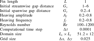
). The physical and numerical parameters are summarized in table 1.
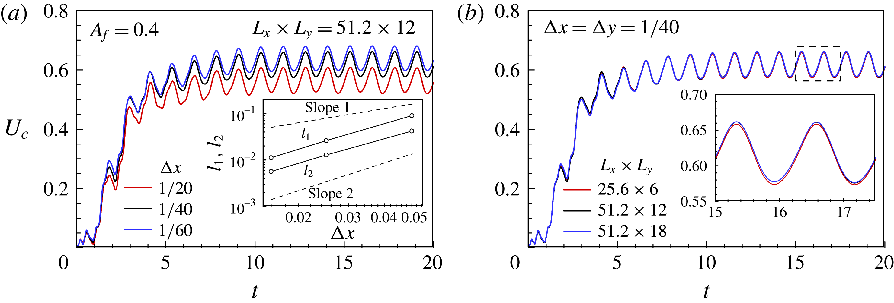
Time histories of the centre velocity
 $U_{c}$
for different (a) grid sizes and (b) domain sizes at
 $Re=100$
. The inset of (a) shows the comparison of the
 $l_{1}$
and
 $l_{2}$
norms for different grid sizes. The inset of (b) shows the magnified view of the centre velocity at
 $15\leqslant t\leqslant 17.5$
.

Physical and numerical parameters.

3 Results and discussion
3.1 Numerical convergence
The centre velocity
 $U_{c}$
of the flexible fin was defined by
 $$\begin{eqnarray}\displaystyle & \displaystyle U_{c}=\int _{0}^{1}\left|\frac{\unicode[STIX]{x2202}X(s,t)}{\unicode[STIX]{x2202}t}\right|\,\text{d}s. & \displaystyle\end{eqnarray}$$
For the isolated fin (IS) (
 $A_{f}=0.4$
and
 $Re=100$
), figure 2(a) shows the time history of the centre velocity
 $U_{c}$
for different grid resolutions, indicating that the velocity difference between
 $\unicode[STIX]{x0394}x=\unicode[STIX]{x0394}y=1/20$
and 1/40 was approximately 9 %. The velocity converged as the grid number increased and a grid size of 1/40 was chosen to save computational costs, where the numerical error was less than 3.5 %. The
 $l_{1}$
and
 $l_{2}$
norms of the error
 $e(t)=\Vert U_{c}(t)-U_{c,r}(t)\Vert$
calculated during
 $0\leqslant t\leqslant 20$
are shown in the inset of figure 2(a), where second-order spatial convergence was achieved.
 $U_{c,r}$
was the centre velocity for a grid resolution of
 $\unicode[STIX]{x0394}x=\unicode[STIX]{x0394}y=1/80$
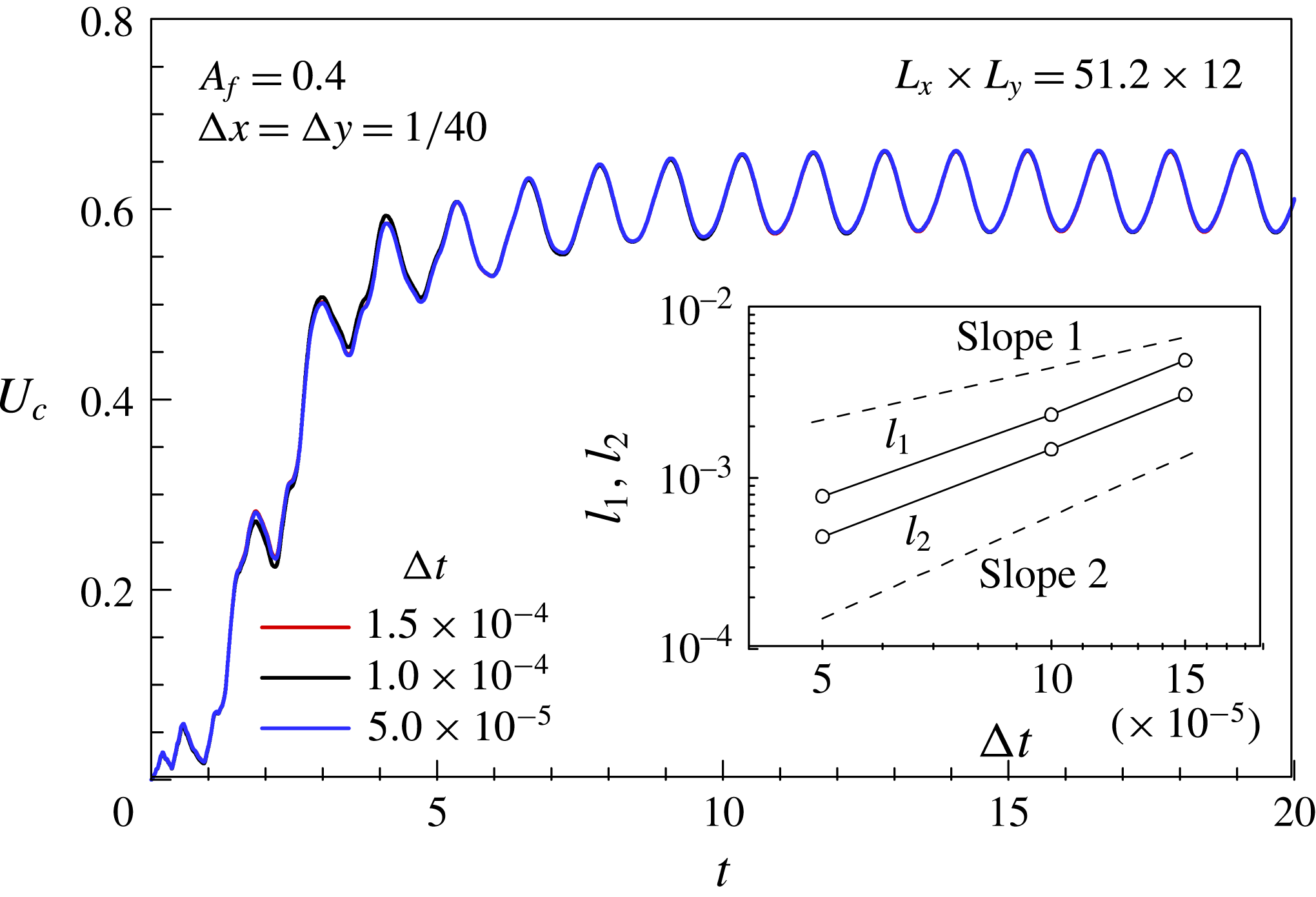
. Figure 2(b) displays the time history of the centre velocity for different computational domains, and the error associated with the domain size used in the present study was less than 0.1 %. Figure 3 shows the convergence test for the time step, and the associated numerical error was less than 0.1 %. The
 $l_{1}$
and
 $l_{2}$
norms were calculated to determine the temporal convergence order, where the centre velocity
 $U_{c,r}$
was for a time step of
 $\unicode[STIX]{x0394}t=2\times 10^{-5}$
. Second-order temporal convergence is shown in the inset of figure 3. Both the spatial and temporal convergence rates corresponded to our numerical discretization schemes (Kim et al.
Reference Kim, Baek and Sung2002).
Time histories of the centre velocity
 $U_{c}$
for different computational time steps at
 $Re=100$
. The inset shows the
 $l_{1}$
and
 $l_{2}$
norms as a function of
 $\unicode[STIX]{x0394}t$
.

3.2 One single fin
A flexible fin swimming in a quiescent flow initially accelerates and reaches a steady state after a few flapping periods. The time-averaged values of the velocity
 $U_{avg}$
and the input power
 $P_{i,avg}$
were measured during the steady state and were obtained by using the following equations:
 $$\begin{eqnarray}\displaystyle & \displaystyle U_{avg}=\frac{1}{T}\int _{t}^{t+T}U_{c}\,\text{d}t & \displaystyle\end{eqnarray}$$
 $$\begin{eqnarray}\displaystyle & \displaystyle P_{i,avg}=\frac{1}{T}\int _{t}^{t+T}P_{i}\,\text{d}t=\frac{1}{T}\int _{t}^{t+T}\int _{0}^{1}\left(\boldsymbol{F}\boldsymbol{\cdot }\frac{\unicode[STIX]{x2202}\boldsymbol{X}}{\unicode[STIX]{x2202}t}\right)\,\text{d}s\,\text{d}t, & \displaystyle\end{eqnarray}$$
where
 $T$
is the flapping period and
 $P_{i}$
is the input power. The Froude efficiency is defined as the ratio of the useful output power to the input power and has been used to quantify propulsive efficiency in some recent studies. However, the resultant force due to the thrust and drag in the streamwise direction is zero for a self-propelled system, which leads to ambiguity in the calculation of the thrust separately from the drag (Park et al.
Reference Park, Chang, Huang and Sung2014). In the previous experimental studies of Thiria & Godoy-Diana (Reference Thiria and Godoy-Diana2010) and Ramananarivo, Godoy-Diana & Thira (Reference Ramananarivo, Godoy-Diana and Thira2011), an additional experiment was performed to measure the thrust force, where the flapping foil was held in a fixed position. The propulsive efficiency was here defined as the ratio of the kinetic energy in the fin forward motion to the work done to the fluid by the fin, which was proposed by Kern & Koumoutsakos (Reference Kern and Koumoutsakos2006) and used in Zhang, Liu & Lu (Reference Zhang, Liu and Lu2010) and Zhu et al. (Reference Zhu, He and Zhang2014a
), Zhu, He & Zhang (Reference Zhu, He and Zhang2014b
). The propulsive efficiency was defined by
 $$\begin{eqnarray}\displaystyle & \displaystyle \unicode[STIX]{x1D702}=\frac{\unicode[STIX]{x1D70C}U_{avg}^{2}}{2TP_{i,avg}}, & \displaystyle\end{eqnarray}$$
where the work done by the flexible fin was calculated by the time integral of the input power. The fin swimming in the wake of other fins necessarily encountered oncoming vortex structures and the work done was affected by how the fin interacted with them. The hydrodynamic advantage or disadvantage of the vortex–body interactions observed in fin schools could be assessed by measuring the propulsive efficiency.
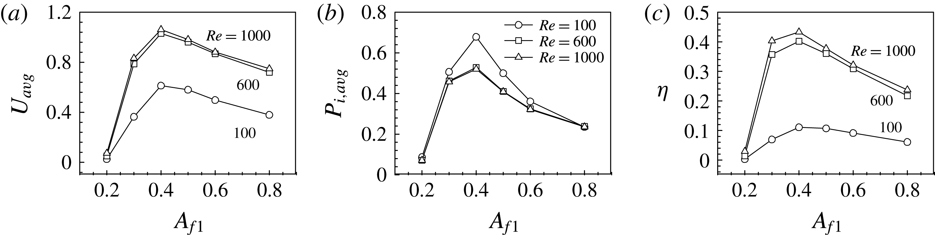
(a) Average velocity, (b) average input power and (c) propulsive efficiency of the single fin as a function of the heaving amplitude.

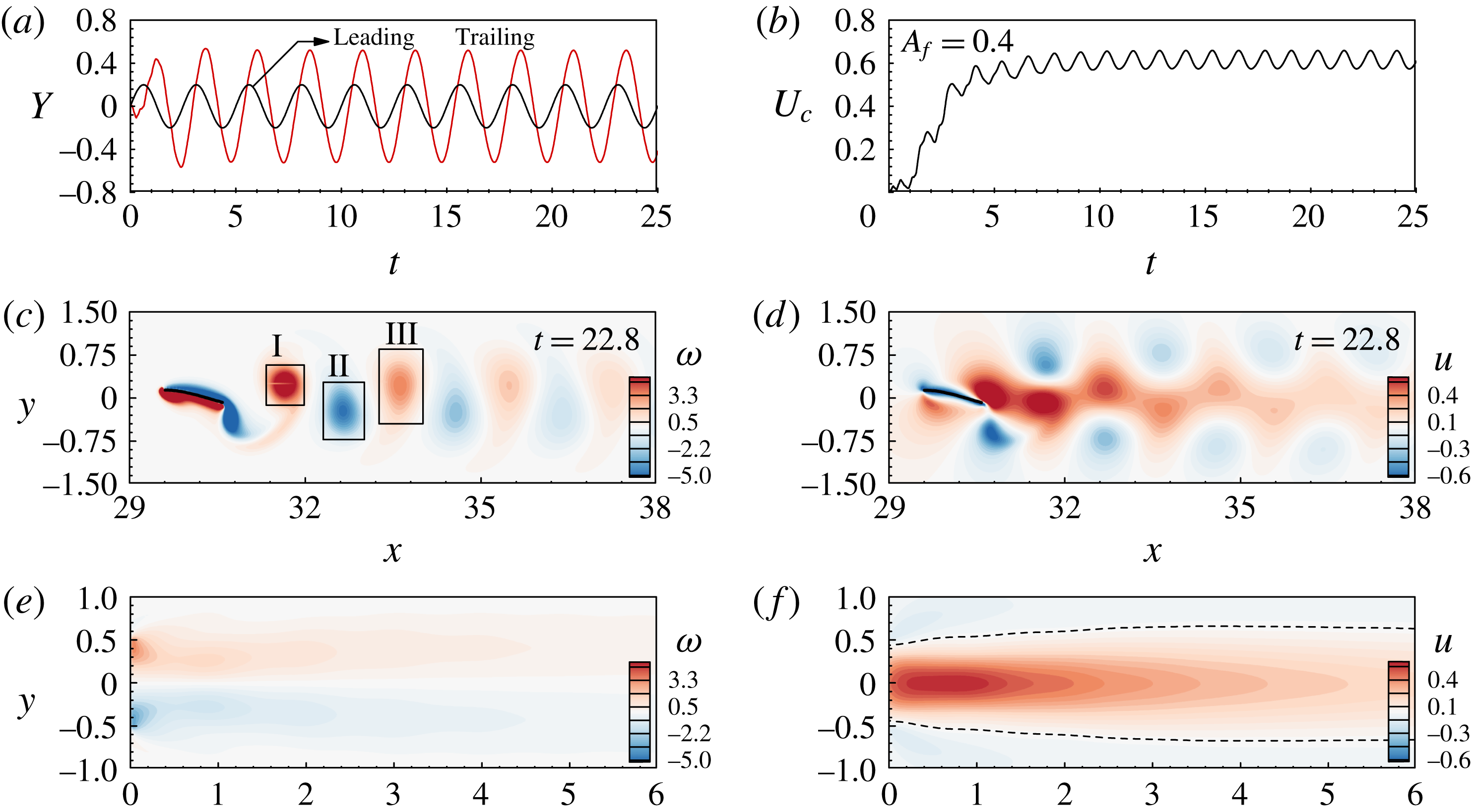
Time histories of (a) the leading and trailing edge
 $y$
-positions and (b) the centre velocity of an isolated fin at
 $Re=100$
. Contours of the (c) instantaneous vorticity and (d)
 $u$
-velocity at
 $t=22.8$
. Contours of the (e) time-averaged vorticity and (f)
 $u$
-velocity over five flapping periods. The flapping amplitude (
 $A_{f}$
) is 0.4.

Figure 4 shows the average velocity, average input power and propulsive efficiency as a function of the heaving amplitude
 $A_{f1}$
for the isolated fin at
 $Re=100$
, 600 and 1000. For the same heaving amplitude, the swimming velocity increases as Re increases in figure 4(a). Figure 4(b) shows that the input power decreases and then converges as Re increases from 100 to 1000, indicating that the viscous effect on the input power is not significant at
 $Re>600$
for the present system. Although a large input power is required, the fin has the highest normalized velocity and exhibits an optimal efficiency for a heaving amplitude of
 $A_{f1}=0.4$
(figure 4
c). For a heaving amplitude of
 $A_{f1}=0.4$
at
 $Re=100$
, figure 5(a) and (b) show the time histories of the leading and trailing edge
 $y$
-positions and the centre velocity
 $U_{c}$
, respectively. The position of the leading edge is determined by the harmonic heaving motion, and other posterior parts flutter passively due to the fluid–flexible-body interactions. The body wave initiated from the leading edge propagates along the flexible fin and reaches the trailing edge with an amplitude of approximately 1.0, as shown in figure 5(a). The fin accelerates initially with the body flapping motion and reaches a steady state in figure 5(b). Figure 5(c,d) show the instantaneous vorticity and
 $u$
-velocity fields, respectively, at
 $t=22.8$
. The fin generates a reverse Kármán vortex street in its wake and a jet-like flow forms near the centre axis. Figure 5(e,f) show the time-averaged vorticity and
 $u$
-velocity fields, respectively, over five flapping periods; a jet-like flow can be seen near the core region. The averaged vorticity fields show that positive and negative vorticity fields occupy the upper and lower areas defined by the centre axis (
 $y=0$
).
3.3 Tandem configuration
Two tandem flexible fins F1 and F2 (
 $G_{y12}=0$
) were simulated at
 $Re=100$
with a heaving motion of
 $A_{f}=0.4$
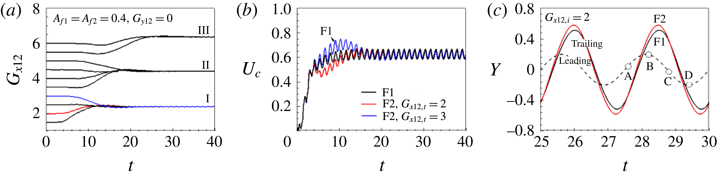
, where the optimal propulsive efficiency was achieved for one single fin. F1 and F2 propelled with the same heaving amplitude of the leading edge without a phase difference. Figure 6(a) shows the time history of the gap distance
 $G_{x12}$
, from which it can be seen that stable tandem configurations spontaneously form between F1 and F2. The discrete equilibrium gap distances were dynamically determined as a function of the initial streamwise gap distance
 $G_{x12,i}$
, as shown in figure 6(a) and supplementary movie 1 available at https://doi.org/10.1017/jfm.2018.64. The time histories of the centre velocities of F1 and F2 are shown in figure 6(b) to visualize the development of the stable configuration. In the tandem configuration, the speeds at which F1 and F2 are propelled are the same during their initial flapping periods. After encountering the vortices shed from F1, F2 experiences an acceleration (blue line) or a deceleration (red line) according to the initial gap distance, and then relaxes to the equilibrium cruising speed. In the stable configurations, F1 and F2 are propelled at the same velocity and maintain their relative positions, but their body kinematics are not the same because they have different fluid environments. For tandem tethered flags flapping in a uniform flow, the flapping amplitude of the downstream flag increases within a specific gap distance range, which leads to an increased drag force known as ‘inverted drafting’ (Ristroph & Zhang Reference Ristroph and Zhang2008; Alben Reference Alben2009; Kim et al.
Reference Kim, Huang and Sung2010). The trailing edge amplitude of F2 increases in figure 6(c), which is similar to the findings of Alben (Reference Alben2009) and Kim et al. (Reference Kim, Huang and Sung2010), and enables F2 to overcome the increased drag force and maintain its position relative to F1.
Time histories of (a) the gap distance
 $G_{x12}$
, (b) the centre velocity and (c) the leading and trailing edge
 $y$
-positions for F1 and F2 in the tandem configuration (
 $G_{y12}=0$
) at
 $Re=100$
. The red and blue lines in (a–c) denote
 $G_{x12,i}=2$
and 3, respectively. Supplementary movie 1 is available online.

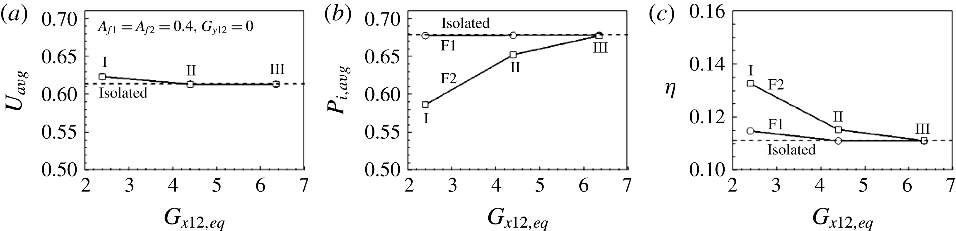
According to the inviscid theoretical model proposed by Weihs (Reference Weihs1973), the following fish in the tandem schooling configuration have to expend extra energy due to the increased relative flow velocity. However, the increased drag does not directly lead to an increased input power, and F2 in the stable tandem configuration reduced its input power by interacting with the oncoming vortices appropriately. Two tandem flexible fins form stable configurations at several discrete equilibrium gap distances (I, II and III in figure 6 a), as discussed by Zhu et al. (Reference Zhu, He and Zhang2014a ). Figure 7 shows the time-averaged velocity, input power and propulsive efficiency during the steady state as functions of the equilibrium gap distance. The two fins in the tandem configuration are propelled at a swimming speed faster than that of an isolated swimmer when they form a stable configuration with a gap distance of approximately 2.4 (I), and they are propelled at almost the same velocity for the gap distances labelled II and III, as shown in figure 7(a). Figure 7(b) shows that F1 benefits little from the tandem configuration in terms of its input power. The input power required for the flapping motion of F2 is reduced by its interactions with the oncoming vortices shed from F1, and those hydrodynamic benefits decrease as the gap distance increases. The efficiency of the following fin F2 is higher than that of the leading fin F1 due to the reduced input power required by F2 (figure 7 c).
(a) Averaged velocity, (b) input power and (c) propulsive efficiency as functions of the streamwise equilibrium gap distance
 $G_{x12,eq}$
between F1 and F2 in a tandem configuration (
 $G_{y12}=0$
).

Fish swimming ahead of their neighbours obtain a benefit from the high-pressure zone created in front of swimming fish, which is similar to that seen for bow-riding dolphins (Fish & Hui Reference Fish and Hui1991; Fish Reference Fish, Domenici and Kapoor2010). Maertens et al. (Reference Maertens, Gao and Triantafyllou2017) found that the leading fish benefit from the tandem schooling configuration due to the increased pressure upstream of the following fish only when they are very close to each other. This effect enables the leader to reduce its flapping amplitude when swimming at the characteristic velocity, and thereby to decrease its input power. Similarly, the presence of F2 assists the propulsion of F1 in the stable tandem configuration with a gap distance labelled I, resulting in an increased swimming velocity rather than a decreased input power. The body wave initiated from the leading edge as the heaving motion propagates along the flexible body induces a transverse flapping motion of the posterior part. The input power is mainly consumed by the generation of transverse body motion. In the tandem configuration, the transverse flapping motion of F1 is only weakly affected by F2, and its input power is almost independent of the position of F2. If, however, F2 swims directly behind F1, it continuously encounters oncoming vortices, which significantly influence its flapping motion. For an identical heaving motion imposed on their leading edges, the input power decreases by up to approximately 14 % for a gap distance labelled I in the stable configuration, and this benefit decreases as the gap distance increases, due to viscosity-induced vortex dissipation. A stable tandem configuration due purely to the hydrodynamic interactions between the two fish becomes less likely as the gap distance increases, because other types of flow perturbation could be predominant.
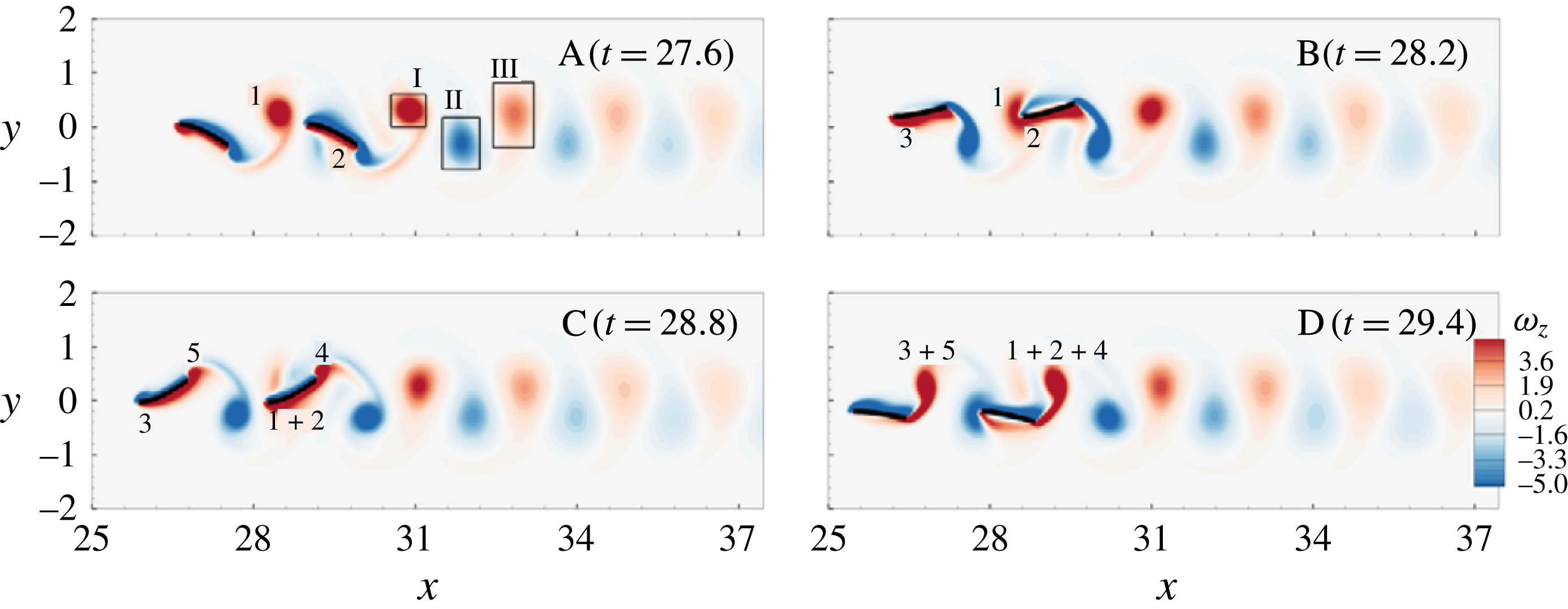
Figure 8 shows the instantaneous vorticity fields at the instants A–D marked in figure 6(c). Positive/negative shear layers have formed on the lower/upper areas along the fin due to the forward motion. In figure 8 at instant A, the positive coherent vortex labelled ‘1’ generated during the downstroke has been shed off the trailing edge of F1. The leading edge of F2 has reached the maximum y-position in figure 8 at instant B, breaking down vortex 1. Vortex 1 has merged into the positive shear layer labelled ‘2’ on the lower part of F2 and dissipated due to the negative shear layer formed on the upper part in figure 8 at instants B and C. The vorticity in the positive shear layer of F2 (
 $1+2$
) is stronger than that of F1 (3) in figure 8 at instant C. As the downstroke proceeds, the shear layers constructively merge into a positive vortex structure at the trailing edge (
 $1+2+4$
). The strengthened vorticity in the shear layer increases the vorticities of the vortex structures denoted I, II and III in figure 8 at instant A as compared to those in the wake of the IS in figure 5(c) (not shown here).
The finite-time Lyapunov exponent (FTLE) field provides a convenient way to reveal the fluid transport barriers, i.e. which fluid particles remain inside or outside the vortex ring (Shadden, Dabiri & Marsden Reference Shadden, Dabiri and Marsden2006). Figure 9 shows the forward FTLE fields for locating Lagrangian coherent structures (LCSs), computed by LCS Matlab Kit developed in the Biological Propulsion Laboratory at California Institute of Technology. The integration length was set to the flapping period
 $|T_{int}|=2.5$
, and the ridges of high FTLE values represent a repelling LCS (Shadden et al.
Reference Shadden, Dabiri and Marsden2006). The repelling LCS (rLCS) visualized between two tandem fins in figure 9 at instant A indicates that the vortex generated by the previous downstroke of F1 (denoted by 1 in figure 8 at instant A) induces the downward flows denoted by the black arrow. The fluid located inside the rLCS over the region of I is detrained and the induced downward flows are encountered by F2 in figure 9 at instants B and C. The rLCS observed beneath F1 in figure 9 at instant A moves downstream as the downstroke proceeds, and the fluid inside the loop (II) is induced to move upwards (denoted by the black arrow) by the vortex structure formed by the upstroke of F1 in figure 9 at instant C.
Instantaneous vorticity fields at the instants A–D (see figure 6
c) for two tandem fins (
 $G_{y12}=0$
).

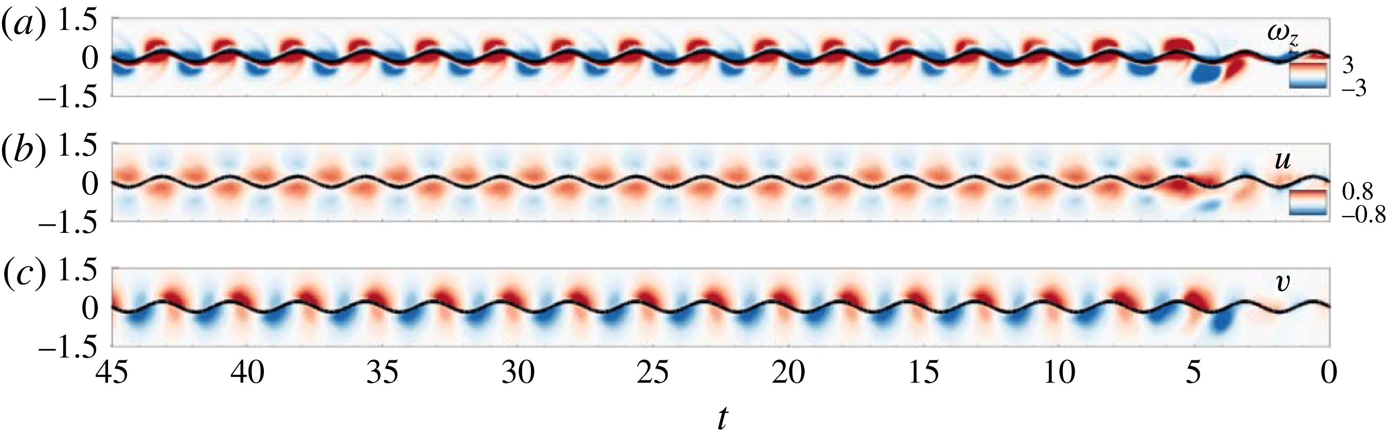
The time evolutions of the vorticity and the u- and v-velocities along the vertical line at the leading edge of F2 are displayed in figure 10 to further visualize the vortex–body interactions of F2. Time evolves from right to left on the
 $x$
-axis. F2 randomly interacts with the oncoming vortices shed from F1 during the initial flapping periods and then a stable configuration is formed. The trajectory of the leading edge of F2 is locked onto the oncoming vortex cores in figure 10(a), which is referred to as the vortex interception mode. The time-averaged field in the wake of the isolated fin indicates that the spanwise range of the positive and negative u-velocity fields is approximately
 $y=\pm 0.5$
, as shown by the dashed line in figure 5(f). The alternating positive and negative vortices shed from F1 form locally distributed positive (the jet-like flow) and negative u-velocity fields, as displayed in figure 10(b). The leading edge of F2 approaches the negative u-velocity field at
 $y=0.2$
and
 $-0.2$
in the vortex interception mode, which minimizes the drag increase due to passing through the jet-like core region. Figure 10(c) shows that the trajectory of the leading edge of F2 is in phase with the induced flow in the spanwise direction, which produces a reduction in the input power required to actuate the heaving motion. The interception mode provides an advantage for F2 in the reverse Kármán vortex street.
FTLE fields at the instants A–C (see figure 6
c) for two tandem fins (
 $G_{y12}=0$
).

Time evolutions of (a) the vorticity, (b) the streamwise velocity and (c) the spanwise velocity along the vertical line at the leading edge of F2 in a tandem configuration (
 $G_{y12}=0$
).

Fish swimming in the wake of a D-cylinder capture energy from oncoming vortices and reduce muscle activity in a vortex exploitation process (Liao et al. Reference Liao, Beal, Lauder and Triantafyllou2003a ). A Kármán vortex street is produced by the D-cylinder, in which the fish slalom between the experimentally generated vortices and activate only their anterior axial muscles. Other posterior parts of the fish flutter passively as a result of the fluid–flexible-body interaction, which leads to a tail amplitude higher than those of fish swimming in a quiescent flow or in a uniform flow without perturbation. Park et al. (Reference Park, Kim and Sung2016) found that a flexible fin swimming in a Kármán gait can maintain its position relative to the upstream cylinder without using any input power by slaloming between the oncoming vortices when the heaving frequency is similar to the vortex shedding frequency. From an energetics perspective, the slaloming between the oncoming vortices provides a hydrodynamic advantage for the fin swimming in the Kármán gait, where the spanwise-induced flows are in phase with the transverse heaving motion (Liao Reference Liao2007; Park et al. Reference Park, Kim and Sung2016). Swimming through the vortex cores is beneficial for F2 in a reverse Kármán vortex street. The vorticity of the flow field in the cylinder wake is strong, so the fin slaloming between the oncoming vortices requires little input power to hold its position. The presence of F2 in the tandem formation reduces the required input power further as the oncoming vortices strengthen.
The phase between the foil motion and the arrival of oncoming vortices is a crucial parameter in vortex–vortex and vortex–body interactions, and thus for the corresponding hydrodynamic benefits (Gopalkrishnan et al. Reference Gopalkrishnan, Triantafyllou, Triantafyllou and Barrett1994; Streitlien & Triantafyllou Reference Streitlien and Triantafyllou1996; Boschitsch, Dewey & Smits Reference Boschitsch, Dewey and Smits2014; Dewey, Quinn & Smits Reference Dewey, Quinn and Smits2014; Uddin et al. Reference Uddin, Huang and Sung2015; Maertens et al. Reference Maertens, Gao and Triantafyllou2017). The phase can be controlled by modulating the flapping motion of the foil itself or the gap distance between the downstream foil and the upstream vortex-generating device, such as a D-section cylinder (Gopalkrishnan et al. Reference Gopalkrishnan, Triantafyllou, Triantafyllou and Barrett1994) or an upstream flapping foil (Uddin et al. Reference Uddin, Huang and Sung2015; Maertens et al. Reference Maertens, Gao and Triantafyllou2017). In one approach, the gap distance was prescribed and the transverse flapping motions were independent of the horizontal propulsion in the tethered system (Uddin et al. Reference Uddin, Huang and Sung2015). In another study, the body kinematics of tandem undulating foils was systematically modified according to changes in the surrounding fluid so that they could swim at a characteristic velocity and maintain a predetermined gap distance (Maertens et al. Reference Maertens, Gao and Triantafyllou2017). The flexible fins modelled here are not as intelligent as the undulating foils of Maertens et al. (Reference Maertens, Gao and Triantafyllou2017) in that the initial heaving amplitudes of the leading edges do not vary once the simulation has started. The posterior parts flutter passively as a result of the fluid–flexible-body interaction, and the cruising velocity is coupled with the flapping motions. The gap distance between F1 and F2 was dynamically determined and stable configurations were found to form spontaneously with the help of F1 via the shared fluid environment. F2 encounters the oncoming vortices with almost the same phase (i.e. the vortex interception mode) regardless of the initial streamwise gap distance and the phase difference between the flapping motions of F1 and F2 by modulating their relative positions (not shown).
3.4 Diagonal configuration
The diagonal configuration is another basic schooling formation. The stable configurations of F1 and F2 were spontaneously determined in the diagonal formation (
 $G_{y12}\neq 0$
) as well as in the tandem formation (
 $G_{y12}=0$
). The initial
 $y$
-positions of the leading edge were
 $y=G_{y12}/2$
and
 $-G_{y12}/2$
for F1 and F2, respectively, as displayed in figure 14. Figure 11 shows the time histories of the gap distance
 $G_{x12}$
in a diagonal configuration for various spanwise gap distances
 $G_{y12}$
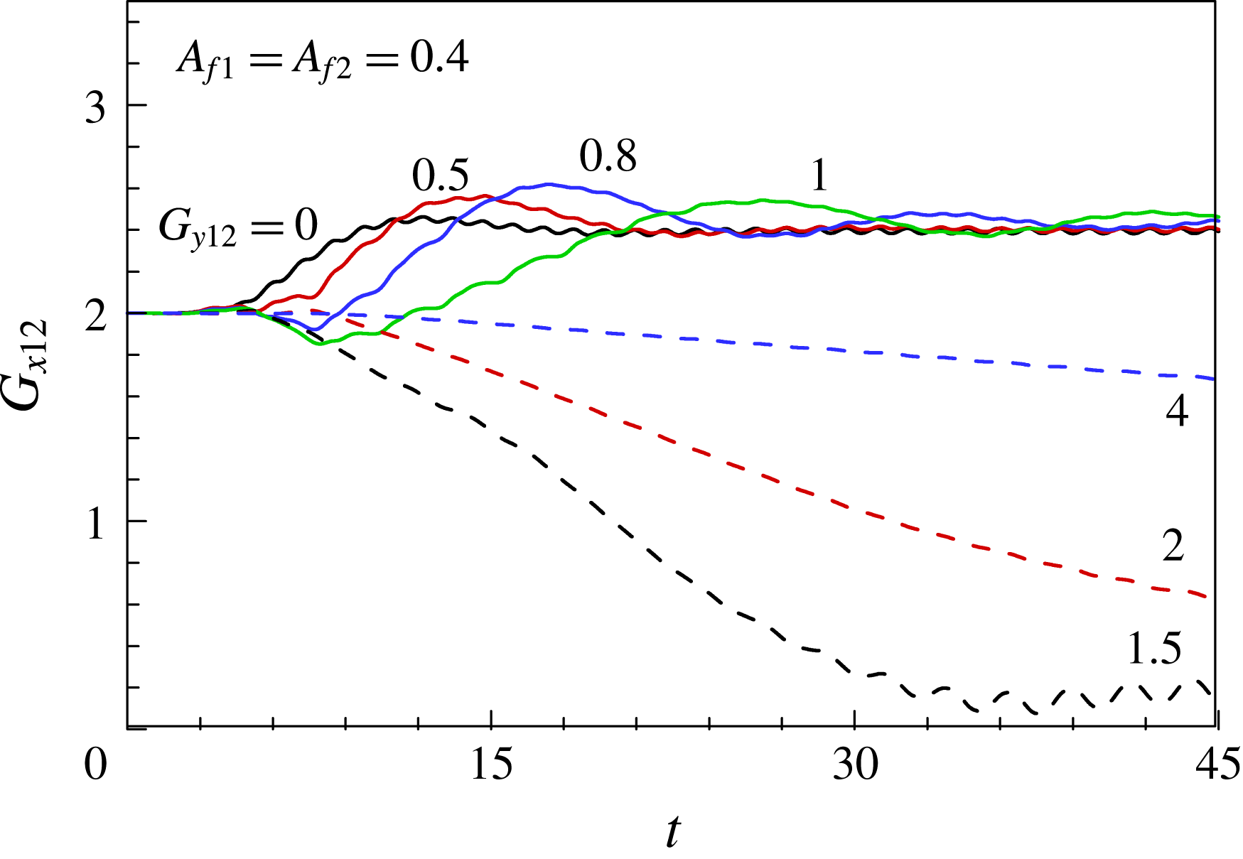
. If the heaving amplitudes of F1 and F2 are the same, the stable diagonal configurations are formed within the spanwise gap distance range
 $0<G_{y12}<0.8$
, where the streamwise gap distances are almost the same as that observed in the tandem configuration (
 $G_{y12}=0$
). When
 $G_{y12}$
is increased to 0.8 and 1, the diagonal configuration becomes unstable and the oscillation amplitude of
 $G_{x12}$
increases. In the case of F2 swimming with
 $G_{y12}>1$
, i.e. outside the jet-like flow region, F2 benefits from the induced flow in the swimming direction and catches up with F1, as shown in figure 11 and supplementary movie 2. The streamwise gap distance decreases and a side-by-side stable configuration is spontaneously formed. The time needed to reach a stable state increases as
 $G_{y12}$
increases.
Time histories of the gap distance
 $G_{x12}$
in a diagonal configuration at
 $Re=100$
for various spanwise gap distances
 $G_{y12}$
. Supplementary movie 2 is available online.

Time histories of (a) the leading and trailing edge
 $y$
-positions and (b) the input power for F1 (black line) and F2 in the tandem (
 $G_{y12}=0$
, red line) and diagonal configurations (
 $G_{y12}=0.5$
, blue line) at
 $Re=100$
.

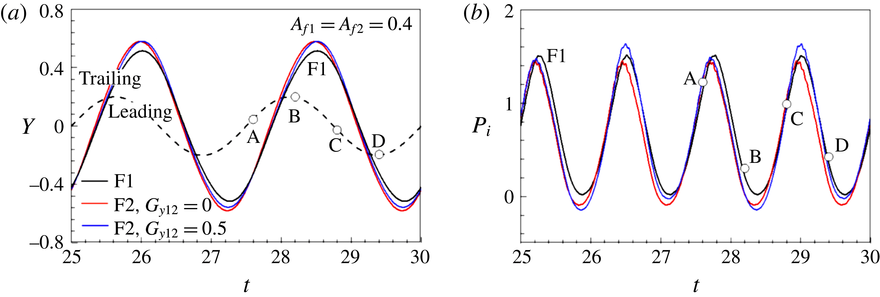
Figure 12(a) shows the time histories of the leading and trailing edge
 $y$
-positions of the fins in the tandem and diagonal configurations. The flapping kinematics of F1 changed only slightly with the relative position of F2. For both configurations, the trailing edge amplitude of F2 increases with respect to that of F1 (black line) due to the vortex–flexible-body interaction. The amplitude of F2 in the tandem configuration (red line) is a little larger than that in the diagonal configuration (blue line). Figure 12(b) shows the time history of the input power, which indicates that F2 requires less input power (red line) than F1 (black line) in the tandem configuration throughout the flapping periods. In the diagonal configuration, F2 (blue line) reduces the input power only in section A–C, and the benefit is noticeable in section B–C. The leading edge of F2 reaches its minimal
 $y$
-position at D, and its trailing edge moves downwards in section C–D, where the required input power is higher than that of F1. Figure 13 shows the averaged values of the velocity, input power and efficiency as functions of
 $G_{y12}$
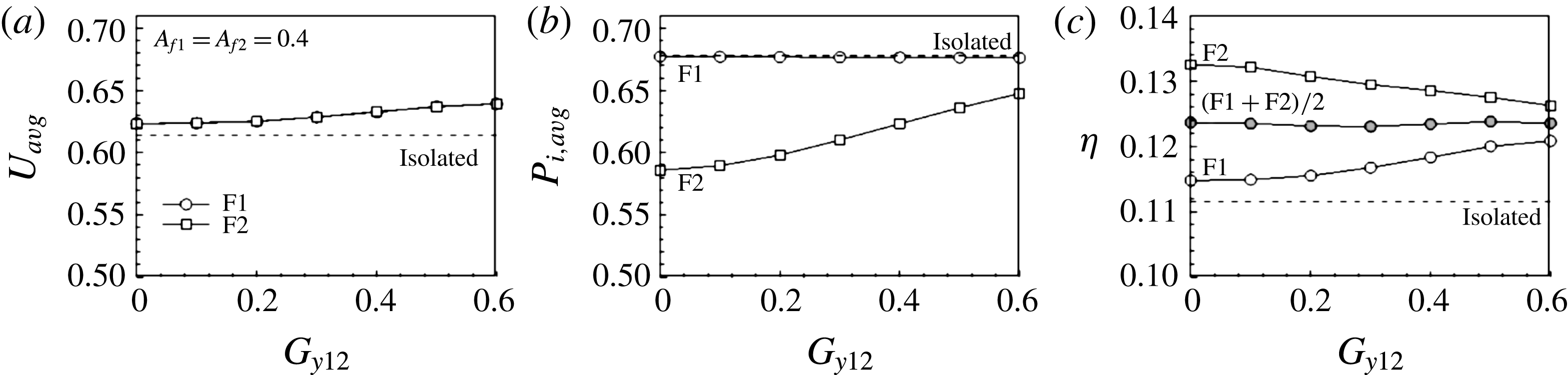
in the stable configuration. Figure 13(a) demonstrates that F1 and F2 swim faster than IS and their velocities increase slightly as
 $G_{y12}$
increases. The required input power of F1 is almost the same as that of IS and varies little with changes in the position of F2, as displayed in figure 13(b). F2 benefits from the wake of F1 in terms of the required input power, which increases as
 $G_{y12}$
increases. In figure 13(c), the efficiencies of F1 and F2 increase and decrease, respectively, with increases in
 $G_{y12}$
. The global efficiency
 $(\unicode[STIX]{x1D702}_{\text{F1}}+\unicode[STIX]{x1D702}_{\text{F2}})/2$
is almost constant and higher than that of IS.
(a) Averaged velocity, (b) input power and (c) propulsive efficiency as a function of the spanwise gap distance
 $G_{y12}$
between F1 and F2 in a diagonal formation. The initial streamwise gap distance
 $G_{x12,i}=2$
.

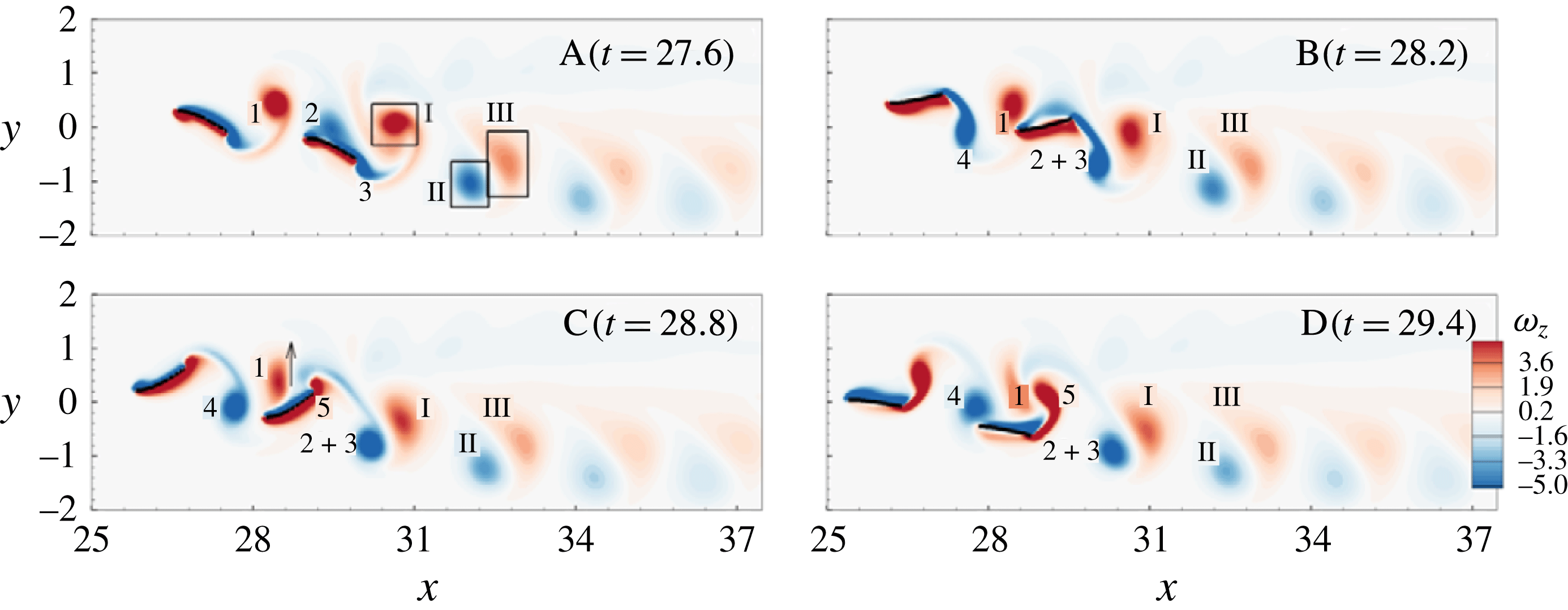
Instantaneous vorticity fields at the instants A–D (see figure 12) for two diagonal fins (
 $G_{y12}=0.5$
).

Figure 14 shows the instantaneous vorticity fields at the instants A–D denoted in figure 12(b). The negative vortex (2) merges into the negative shear layer formed on the upper part of F2, as shown in figure 14 at instant A. The merged negative shear layer grows along the body and is shed by the trailing edge as the coherent structure (
 $2+3$
) during the upstroke of F2, as shown in figure 14 at instants B and C. F2 passes below the positive vortex (1), which was encountered by the negative shear layer on the upper part of F2, as can be seen in figure 14 at instant B. The positive vortex moves from the leading edge to the middle part of F2 in section B–C and induces the upward flow marked by the arrow in figure 14 at instant C. F2 performs a downstroke during B–C and the large input power required for the flapping motion during this period (figure 12
b) is possibly due to the upward induced flow. In figure 14 at instant D, the positive vortex (1) formed by F1 amalgamates with another positive vortex (5) near the trailing edge of F2. The downstream movement of the positive vortex (5) is temporarily retarded and its circulation intensifies as it merges with the positive vortex (1). The wake symmetry is broken due to the retardation of the positive vortex structure (
 $1+5$
). The symmetry-breaking velocity induced by vortex dipoles II and III is larger than the symmetry-holding velocity induced by vortex dipoles I and II due to the increased gap distance between I and II, as shown in figure 14 at instant A. The negative vortex (
 $2+3$
) was deflected downwards rapidly and interacts with the positive vortex (I) as soon as it is shed by the trailing edge of F2. Figure 15 shows the forward FTLE field for two diagonal fins (
 $G_{y12}=0.5$
). The fluid located in the region of I is detrained out of the rLCS and downward motion of the fluid is induced (the black arrow), while the fluid in the region of III remains inside the rLCS and interacts with F2 in its upper part as the upstroke proceeds in figure 15 through instants A, B and C. The fluid located inside the loop (II) in the lower region of F1 is detrained as the upstroke proceeds, producing an upward motion of the fluid, as denoted by the black arrow in figure 15 at instant C.
FTLE fields at the instants A–C (see figure 12) for two diagonal fins (
 $G_{y12}=0.5$
).

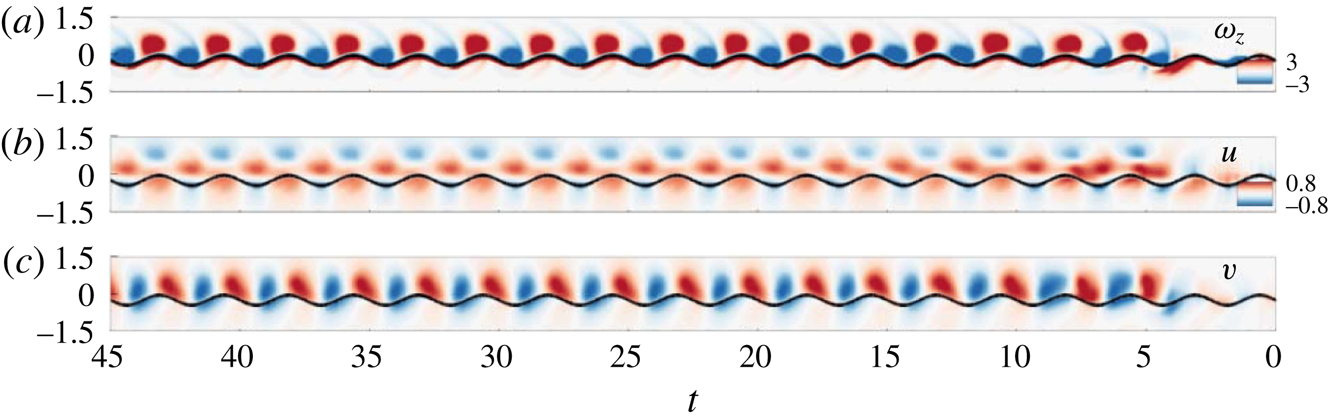
Time evolutions of (a) the vorticity, (b) the streamwise velocity and (c) the spanwise velocity along the vertical line at the leading edge of F2 in a diagonal configuration (
 $G_{y12}=0.5$
).

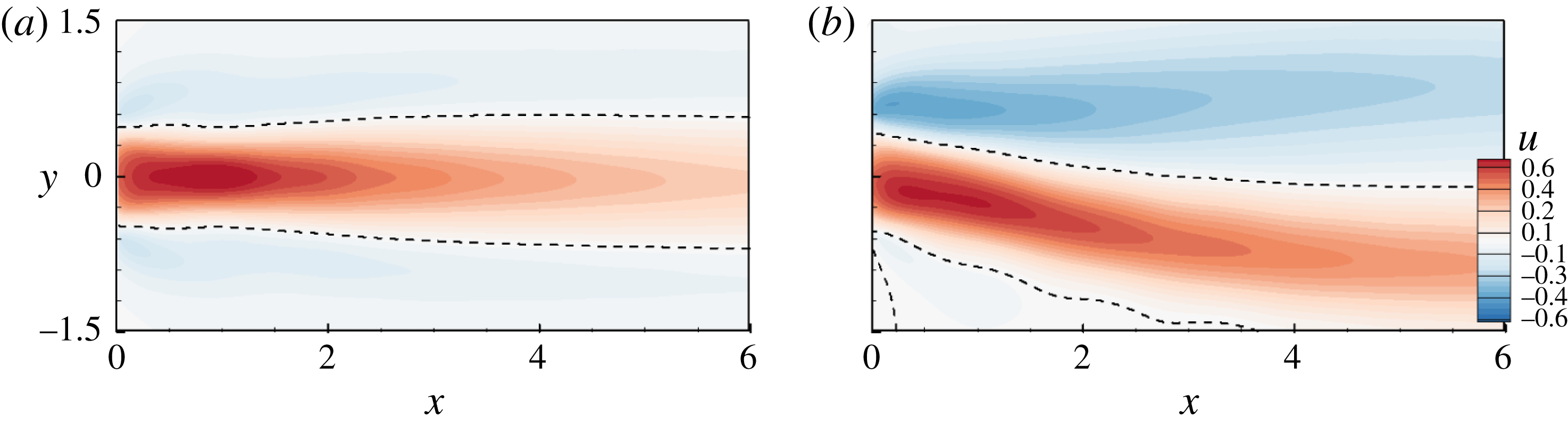
Figure 16 shows the time evolutions of the vorticity and the u- and v-velocities along the vertical line at the leading edge to visualize how F2 exploits the oncoming vortices in the stable diagonal configuration. F2 reaches a steady state after a few initial flapping periods, and its leading edge passes over the lower parts of the positive and negative vortices in the stable configuration. In figure 16(b), the leading edge passes through the flows that are induced in the swimming direction by the negative oncoming vortices, which reduces the drag increase resulting from passing through the jet-like flows near the centre axis. The motion of the leading edge and the induced flows are synchronized in the spanwise direction, as shown in figure 16(c). In the stable tandem configuration in figure 8 (instant C), the induced flows in the spanwise direction play the role of a ‘hydrodynamic puller’: positive and negative spanwise flow regions form on the upper and lower parts of the leading edge trajectory, respectively, and act as if they are pulling the leading edge, which reduces the input power. On the other hand, when F2 is in the wake of F1 diagonally, it passes over the lower parts of the positive and negative induced flows in the y-direction. The positive and negative flows play pulling and pushing roles, respectively. Both effects reduce the input power required of F2, which as a result is less than that of IS during the initial downstroke of the leading edge, as shown in section B–C in figure 11(b). The leading edge benefits from hydrodynamic pushing in section C–D, but the positive oncoming vortex hinders the downward flapping motions of other posterior parts, which increases the required input power rapidly, as visualized in figure 14.
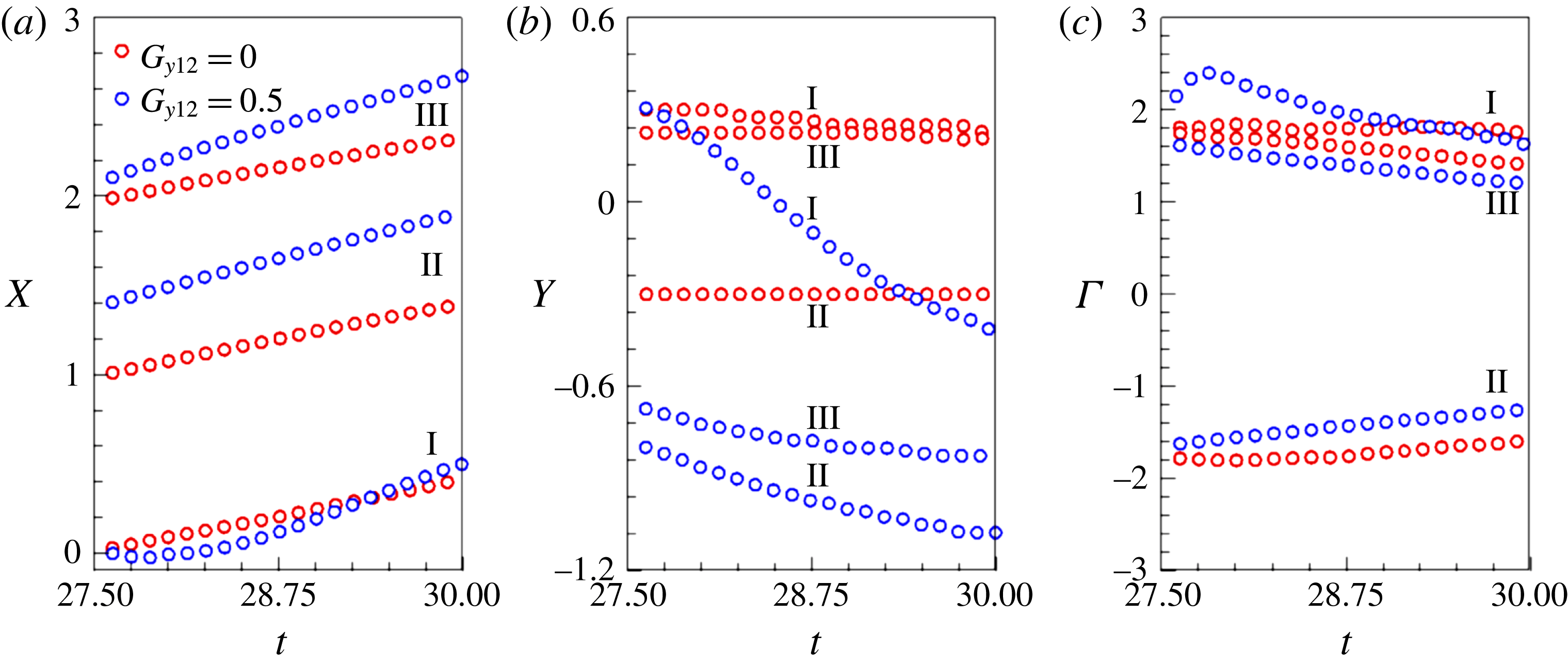
Figure 17(a) shows the time histories of the vortex structure x-positions relative to the trailing edge; the red and blue symbols are for the tandem and diagonal configurations, respectively. For
 $G_{y12}=0.5$
, vortex I drifts downstream more slowly during the initial flapping periods than for
 $G_{y12}=0$
, and accelerates after the merging process is finished. The momentum transfer that results from the diagonal positioning of F2 in the wake of F1 is higher, and the vortices (I, II and III) move downstream more rapidly than for the tandem configuration. The increased swimming velocities of F1 and F2 in the diagonal formation are attributed to the increased streamwise momentum transferred to the surrounding fluid. Figure 17(b) demonstrates that the absolute
 $y$
-positions of the vortices (I, II and III) are almost the same as in the tandem formation, which can be characterized by a symmetric wake structure. In the diagonal configuration, the y-positions indicate that the structures are initially deflected downwards and then drift downstream while maintaining their horizontal levels. Figure 17(c) shows the time histories of the vortex circulation, which reveal that the circulation of vortex I is intensified by the merging process. The dissipation rate of the structures in the diagonal configuration is higher than that of the tandem configuration. Figure 18 shows the time-averaged
 $u$
-velocity fields in the wake of F2 for the tandem (
 $G_{y12}=0$
) and diagonal (
 $G_{y12}=0.5$
) configurations. Figure 18(a) demonstrates that the time-averaged velocity field of the tandem configuration is analogous to that of IS, for which jet-like flows form near the core region, and that outside the core region flows are induced in the swimming direction. In the diagonal configuration (figure 18
b), the jet-like flows are deflected downwards and negative
 $u$
-velocity regions are distributed near the core region.
Time histories of the positions and circulations of the vortices: (a) x-positions relative to the trailing edge; (b) y-positions relative to the symmetric axis of the heaving motion; (c) circulations. Red and blue symbols denote
 $G_{y12}=0$
and 0.5 respectively.

Time-averaged
 $u$
-velocity contours in the wake of F2 for (a)
 $G_{y12}=0$
and (b)
 $G_{y12}=0.5$
.

The swimming of F2 in the stable tandem or diagonal configurations requires less input power than that of F1 because it can exploit oncoming vortices. We found that there is a trade-off between the efficiencies of F1 and F2 in the stable diagonal configuration that enables them to maintain a global efficiency that is approximately 10 % higher than that of IS (figure 13
c). The hydrodynamic benefits of F2 swimming through the vortex centres in the reverse Kármán gait decrease as the spanwise gap distance increases when F1 and F2 swim with the same heaving amplitude. This tendency in the hydrodynamic benefit of the following fin with the spanwise offset is contrary to the findings of Maertens et al. (Reference Maertens, Gao and Triantafyllou2017), where the following fin swimming in the reduced velocity region of the wake could take advantage of the spanwise offset to reduce the flapping amplitude, further decreasing the input power. The swimming of fish behind two adjacent fish requires less energy due to the reduced flow region according to the inviscid theory (Weihs Reference Weihs1973). F2 is more likely to pass through the negative u-velocity region because of the spanwise offset, as shown in figure 16(b), which alleviates the increased drag associated with the jet-like flow region near the centre axis. The decrease in the input power required of the following fish that results from the spanwise offset mainly arises as a reduced flapping amplitude rather than as a direct result of the hydrodynamic interaction according to Maertens et al. (Reference Maertens, Gao and Triantafyllou2017). The benefits resulting purely from hydrodynamic interactions diminish as the spanwise distance increases. The input power required by F2 to swim in the diagonal formation with
 $G_{y12}=0.5$
is lower by 6 % than that of F1 and higher by 9 % than that of F2 in the tandem formation (
 $G_{y12}=0$
).
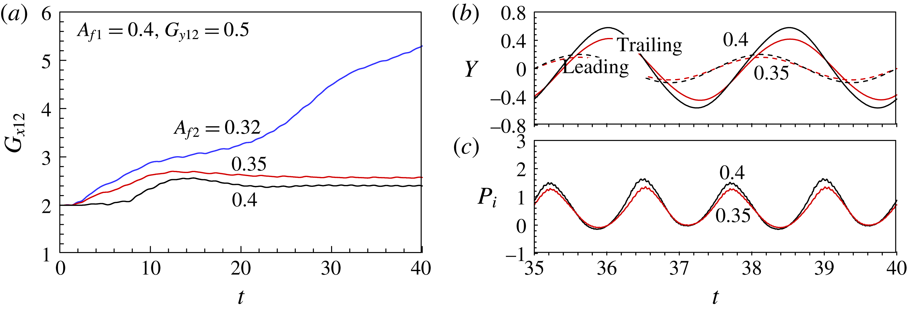
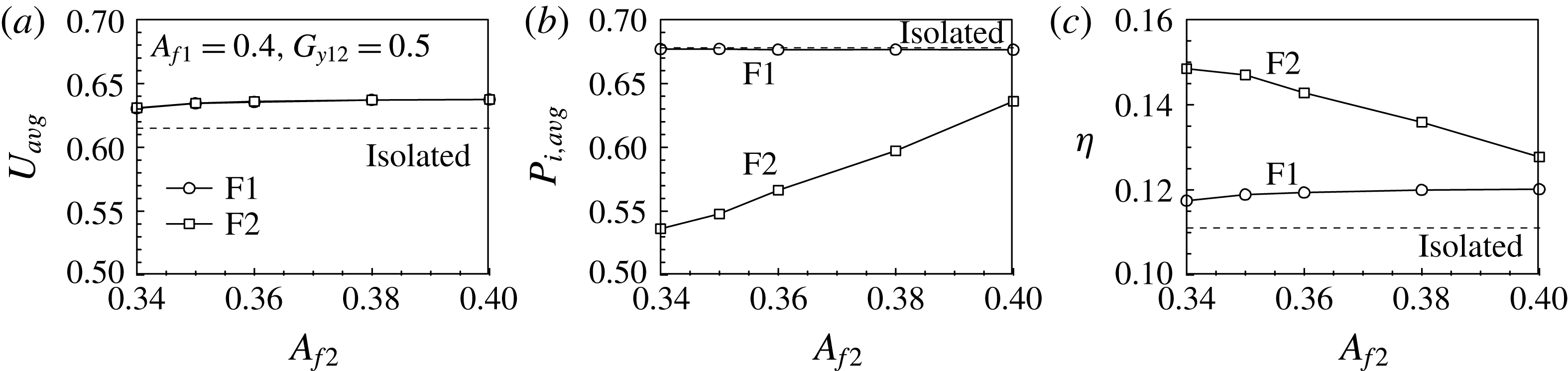
Figures 19 and 20 show the effects of varying the F2 heaving amplitude in the stable diagonal configuration in order to determine whether F2 can follow F1 with a reduced heaving amplitude on the leading edge and thus optimize the propulsive efficiency by diminishing its input power further. The heaving amplitude of F1 was fixed at
 $A_{f1}=0.4$
, so only that of F2 decreases in these figures. In figure 19(a), F2 flapping with
 $A_{f2}=0.32$
is unable to follow the leader, and the gap distance increases, whereas F2 with
 $A_{f2}=0.35$
can follow F1, and the stable configuration forms spontaneously. Both the trailing edge amplitude and the input power required for the flapping motion are reduced by decreasing the heaving amplitude of F2. Figure 20 shows the averaged velocity, input power and efficiency for the stable configuration as functions of the F2 heaving amplitude. The velocity is higher than that of IS and decreases slightly as the heaving amplitude of F2 decreases. The input power required by F2 is lower by 6 % than that of F1 for the same heaving amplitude, and an input power saving of 21 % is possible for the reduced heaving amplitude
 $A_{f2}=0.34$
. Thus the benefits associated with the reduced heaving motion dominate those of the vortex–vortex and vortex–flexible-body interactions. The required input power decreases and the efficiency increases as the F2 heaving amplitude decreases. The following fin swimming diagonally behind the leading fin can sustain the configuration with the reduced flapping amplitude, which can be explained by drag reduction induced from undulating in the reduced velocity wake region (Maertens et al.
Reference Maertens, Gao and Triantafyllou2017). The hydrodynamic benefits of F2 resulting purely from the vortex–body interactions are diminished as the spanwise gap distance increases, implying that reducing the flapping amplitude is not an option but a necessity for the following fish swimming diagonally behind the leader to enhance the propulsive efficiency.
Time histories of (a) the gap distance
 $G_{x12}$
, (b) the leading and trailing edge
 $y$
-positions and (c) the input power for F2 in the diagonal configuration (
 $G_{y12}=0.5$
) at
 $Re=100$
. The reduced heaving amplitudes of F2 are superimposed: black line (
 $A_{f1}=A_{f2}=0.4$
), red line (
 $A_{f2}=0.35$
) and blue line (
 $A_{f2}=0.32$
).

(a) Averaged velocity, (b) input power and (c) propulsive efficiency as a function of the heaving amplitude of F2. The spanwise gap distance is
 $G_{y12}=0.5$
.

3.5 Triangular configuration
The
 $u$
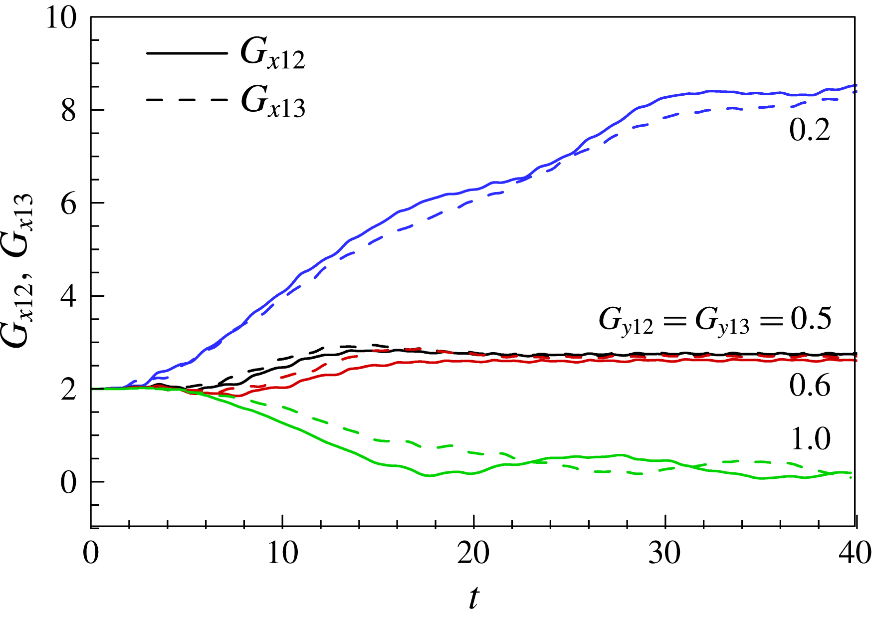
-velocity field for the stable diagonal configuration suggests the possibility of another schooling configuration that could spontaneously form as a result of vortex–vortex and vortex–flexible-body interactions. Supplementary movie 3 shows that a third fin F3 diagonally in the wake of F1 and F2 could follow F2 and that a stable triangular configuration then forms that retains the relative positions among F1, F2 and F3. Figure 21 shows the time histories of the gap distances
 $G_{x12}$
and
 $G_{x13}$
as functions of
 $G_{y12}$
and
 $G_{y13}$
. The three fins were initially positioned in the triangular configuration to reduce the computational time required to reach a steady state. F2 and F3 are positioned symmetrically to the centre axis, i.e.
 $G_{y12}=G_{y13}$
, as displayed in figure 1. Increasing the population in a fish school increases the complexity of the system. F1 and F2 form a stable diagonal configuration when
 $G_{y12}=0.2$
. However, F2 and F3 in the wake of F1 with
 $G_{y12}=G_{y13}=0.2$
are not able to follow the leader, so
 $G_{x12}$
and
 $G_{x13}$
increase in figure 21 and supplementary movie 4. When the heaving amplitudes of the leading edges of F2 and F3 are the same, a side-by-side configuration forms for
 $G_{y12}>1$
and a stable triangular configuration for
 $0.4\leqslant G_{y12}(=G_{y13})\leqslant 0.6$
, with a dynamically determined streamwise gap distance of approximately
 $G_{x,eq}=2.7$
.
Time histories of
 $G_{x12}$
and
 $G_{x13}$
for various
 $G_{y23}$
values in the triangular configuration at
 $Re=100$
. The initial streamwise gap distance is
 $G_{x12,i}=G_{x13,i}=2$
. Supplementary movie 4 is available online.

Time histories of (a) the leading and trailing edge
 $y$
-positions and (b) the input powers for the fins in the triangular configuration (
 $G_{y12}=G_{y13}=0.5$
) at
 $Re=100$
.

Figure 22 shows the time histories of the leading and trailing edge
 $y$
-positions and the input powers for the three fins in the stable triangular configuration with
 $G_{y12}=G_{y13}=0.5$
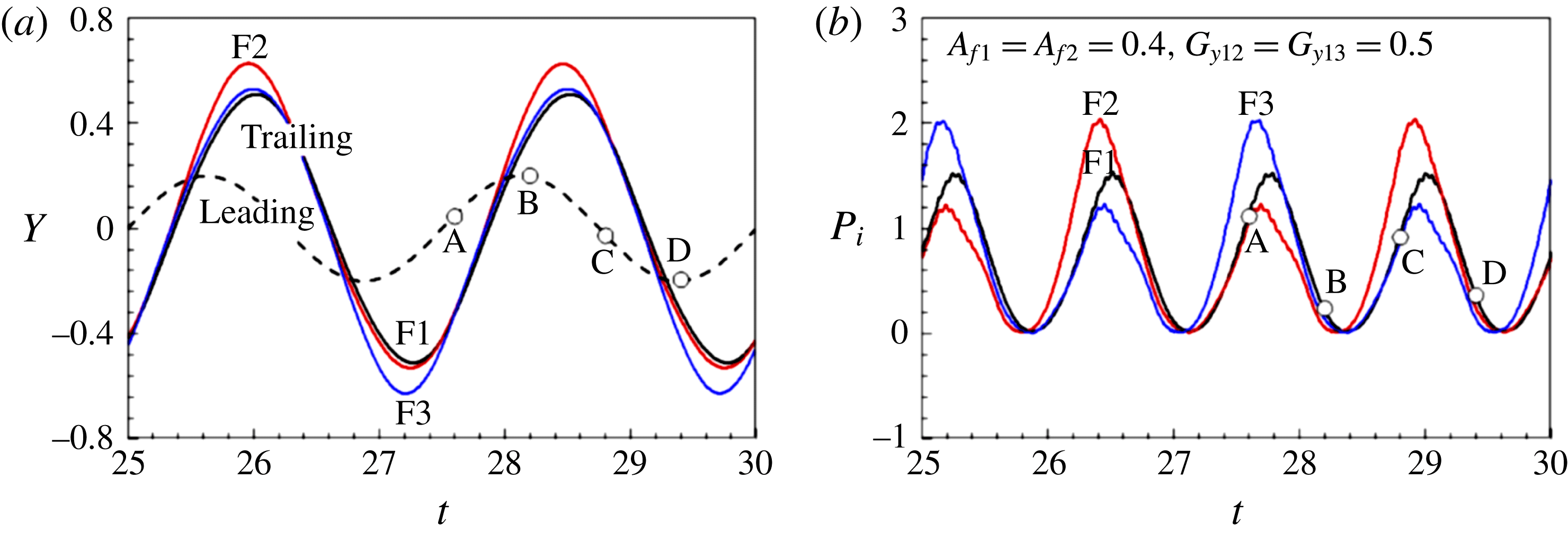
. F2 is positioned in the lower part of the second row; its trailing edge amplitude becomes greater than those of F1 and F3 during the upstroke. F3 is positioned in the upper part of the second row and performs a downstroke with increased trailing edge amplitude in figure 22(a). The input powers required for the upstrokes and downstrokes of F1 are the same for this symmetric flapping motion based on the heaving axis, whereas those of F2 and F3 are different because their motions are asymmetric. Figure 22(b) indicates that F2/F3 spent more/less energy during the downstroke (section B–D) than the upstroke. The input power of F2 (or F3) is affected by F3 (or F2) and the oncoming vortices shed from F1. Figure 23 shows the instantaneous pressure field at A (
 $t=27.6$
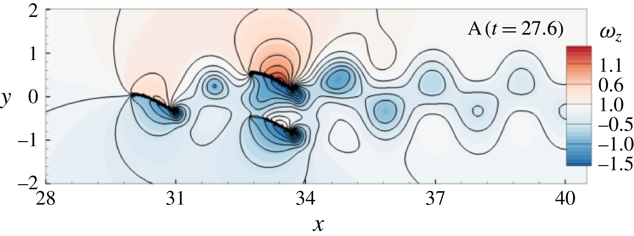
), where the fins are performing an upstroke. Positive and negative pressure fields are induced during the upstroke over the upper and lower parts of the fin, respectively. In figure 23, negative pressure is created between F2 and F3 due to the upward flapping motion of F3, which reduces the input power of F2 and increases the trailing edge of F2, as shown in figure 22. The increment in the input power required by F3 during the upstroke is attributed to the increased pressure field on the upper part of F3.
Instantaneous pressure field at A (
 $t=27.6$
). The line contour level is 0.2.

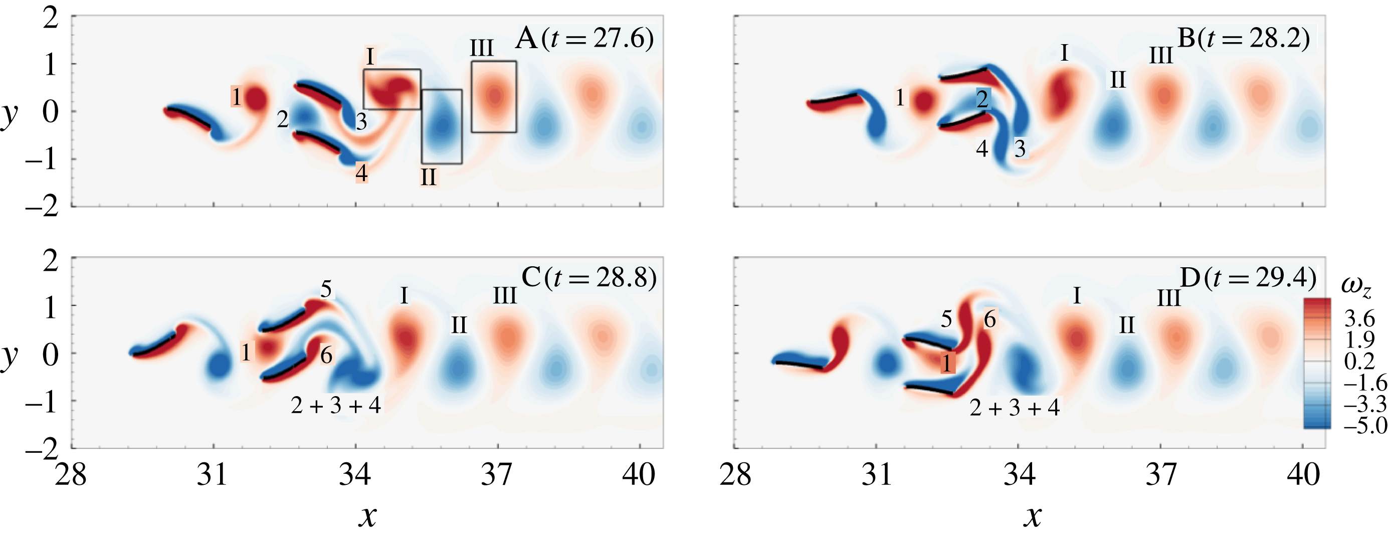
Figure 24 shows the instantaneous vorticity fields at the instants A–D. During one flapping period, only one pair of positive and negative vortex structures is evident in the wake of the three fins swimming in the stable triangular configuration. As shown in figure 24 at instants A and B, the negative vortex oncoming from F1 merges into the negative shear layer formed on the upper part of F2, which is analogous to the merging process observed in the diagonal configuration. The negative vortices 3 and 4 are generated by the upstrokes of F3 and F2, respectively, and shed off their trailing edges as they merge. Vortex 2 moves along F2 and is amalgamated into the negative vortices to form
 $2+3+4$
in figure 24 at instant C. The positive oncoming vortex (1) moves along F3 (not F2) and merges into the positive vortices (5 and 6) generated by the downstrokes of F3 and F2.
Instantaneous vorticity fields at the instants A–D in figure 22 for three triangular fins (
 $G_{y12}=G_{y13}=0.5$
).

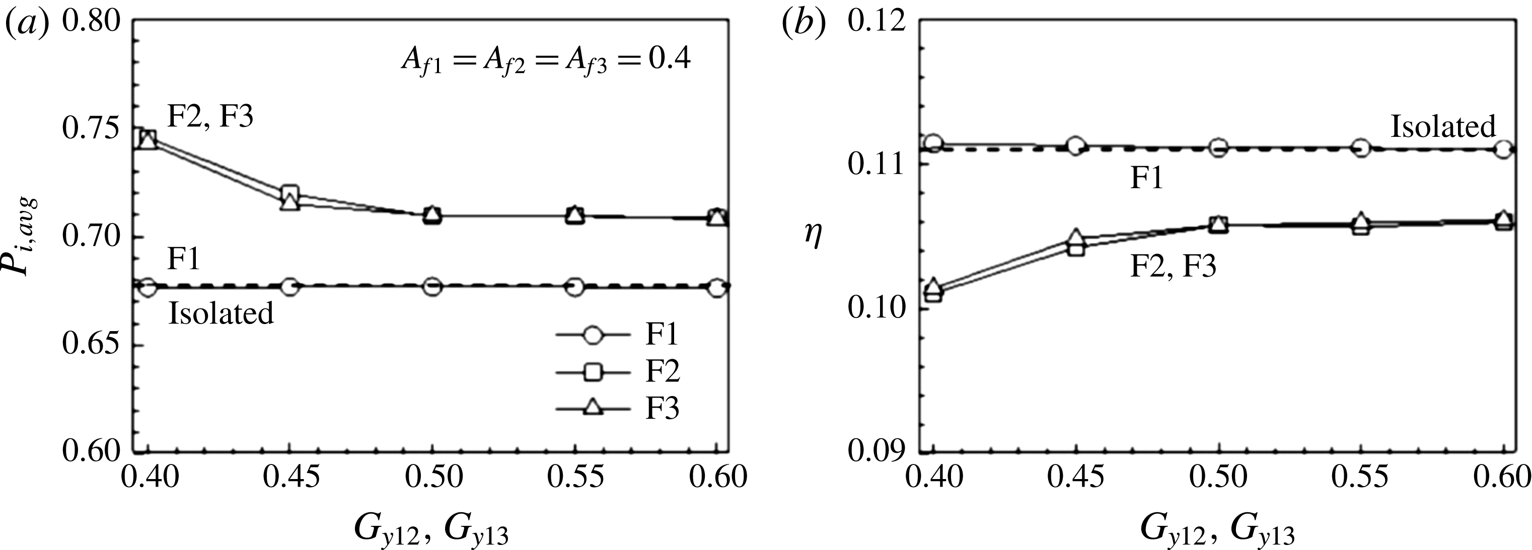
Figure 25 shows the input power and the efficiency as functions of the spanwise gap distance in the stable triangular configuration. The cruising velocity of the school is the same as that of IS, and varies little with the spanwise gap distance. Figure 25(a) indicates that the input power of F1 is similar to that of IS, whereas F2 and F3 require more input power to swim at the same velocity, which leads to the decrease in efficiency in figure 25(b). F2 and F3 need to reduce the heaving amplitude to save input power and mitigate the penalty of the increased input power induced from swimming in the second row of the triangular configuration. F2 and F3 are able to follow F1 and form a stable configuration with reduced heaving amplitudes
 $0.34\leqslant A_{f2}(=A_{f3})\leqslant 0.4$
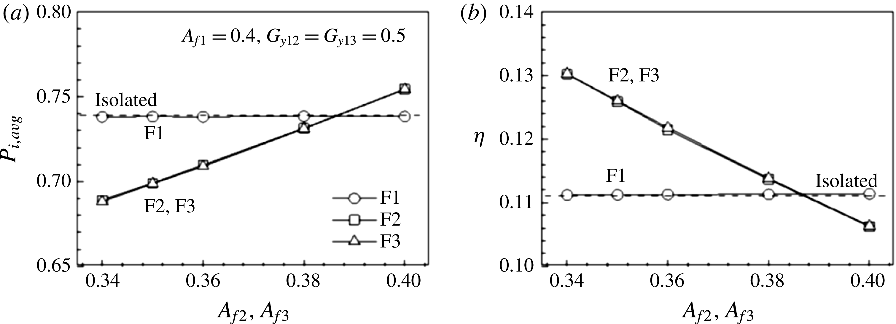
; at lower amplitudes a stable triangular configuration cannot form. F2 and F3 propel with the same velocity and maintain their relative positions to F1 despite their decreased heaving amplitudes as compared to that of F1. The input powers of F2 and F3 decrease as the heaving amplitudes decrease, as shown in figure 26(a). The individual efficiencies of F2 and F3 increase by up to approximately 18 % with the decreases in the heaving amplitudes in figure 26(b).
(a) Input power and (b) efficiency as a function of the spanwise gap distances
 $G_{y12}$
and
 $G_{y13}$
in the triangular configuration.

(a) Input power and (b) efficiency as a function of the heaving amplitudes of F2 and F3 in the triangular configuration.

Two tandem flexible propulsors with paddling-based locomotion produce a stable configuration and their average cost of transport is less than that of an isolated propulsor (Park & Sung Reference Park and Sung2016). The leading propulsor benefits from the increased pressure region formed in front of the following propulsor during the contraction period, while the follower is hindered by the increased pressure region inside the leader’s bell. In contrast, the leader assists the propulsion of the follower during the relaxation phase. Similarly, F2 benefits from the low-pressure region between F2 and F3, which reduces the required input power during the upstroke, whereas a higher input power is required for F3. During the downstroke, the presence of F2 means that F3 can reduce its input power at the expense of an increase in the input power required by F2. The input powers of F2 and F3 during the whole flapping period exceed that of F1 by 5 %, which results from the flow-mediated interaction. A stable triangular configuration with F2 and F3 swimming in the second row with diminished heaving amplitudes is formed, which means that they use less energy than the leader.
(a) Time histories of the gap distances
 $G_{x12}$
,
 $G_{x13}$
and
 $G_{x14}$
for various spanwise gap distances in the diamond configuration at
 $Re=100$
. The red, black and blue lines denote
 $G_{y12}(=G_{y13})=0.4$
, 0.5 and 0.6, respectively. Supplementary movie 5 is available online. (b) Time histories of the gap distance
 $G_{x12}$
,
 $G_{x13}$
and
 $G_{x14}$
for various heaving amplitudes in the diamond configuration (
 $G_{y12}=G_{y13}=0.5$
). The red, black and blue lines denote
 $A_{f1}=0.2$
, 0.4 and 0.5, respectively.

3.6 Diamond configuration
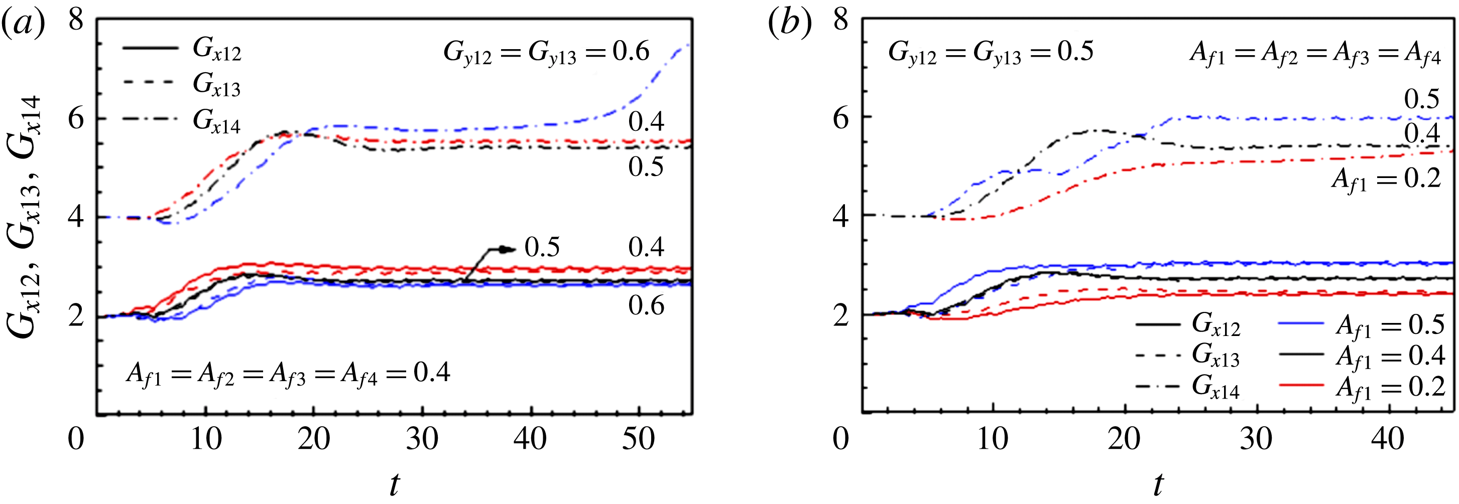
In the stable tandem configuration, the follower maintains its position relative to the leader in the reverse Kármán vortex street. We found that the wake features of the three fins swimming in the stable triangular configuration are very similar to those of IS and the fourth fin (F4) swimming on the same horizontal level, as F1 in the third row was observed to maintain its position relative to the leading individuals, which creates a stable diamond formation, as presented in Supplementary movie 5. Figure 27(a) shows the time histories of
 $G_{x12}$
,
 $G_{x13}$
and
 $G_{x14}$
for four fins initially positioned in the diamond configuration with
 $G_{x12,i}=G_{x13,i}=G_{x24,i}=2$
and various spanwise gap distances. For the synchronized heaving motion (
 $A_{f}=0.4$
), the diamond configuration forms for
 $0.4\leqslant G_{y12}(=G_{y13})<0.6$
. F1, F2 and F3 form a triangular configuration and F4 cannot catch up with them for
 $G_{y12}=G_{y13}=0.6$
. The flapping motion of the flexible fin is mainly determined by the heaving amplitude imposed on the leading edge, which is an important factor for achieving the stable configurations. Biological swimmers generally operate at a flapping amplitude of approximately 0.2, which is normalized by body length (Gazzola, Argentina & Mahadevan Reference Gazzola, Argentina and Mahadevan2014a
). A rainbow trout swimming in a free stream with a flapping amplitude of approximately 0.2 (normalized by body length) adjusted its flapping motion appropriately to the oncoming vortices when swimming in the wake of a D-section cylinder, where the flapping amplitude increased to approximately 0.7 (Liao et al.
Reference Liao, Beal, Lauder and Triantafyllou2003a
,Reference Liao, Beal, Lauder and Triantafyllou
b
). Figure 27(b) displays the streamwise gap distances
 $G_{x12}$
,
 $G_{x13}$
and
 $G_{x14}$
as a function of the time for various heaving amplitudes in the diamond configuration, where the spanwise gap distance was
 $G_{y12}=G_{y13}=0.5$
. The stable diamond configurations (
 $G_{y12}=G_{y13}=0.5$
) are formed for flexible fins flapping with a heaving amplitude of
 $0.3\leqslant A_{f1}\leqslant 0.5$
, when the heaving amplitudes are the same for all the members. The fins flapping at
 $A_{f}=0.2$
form a stable triangular configuration and the trailing fin (F4) is not able to follow the upstream fins, increasing the streamwise gap distance
 $G_{x14}$
as shown in figure 27(b). This implies that fish swimming in a group should modulate their flapping amplitudes appropriately to sustain stable configurations purely resulting from their flow-mediated interactions, similar to the rainbow trout swimming behind a D-section cylinder, which increased the flapping amplitude and exploited oncoming vortices (Liao et al.
Reference Liao, Beal, Lauder and Triantafyllou2003a
,Reference Liao, Beal, Lauder and Triantafyllou
b
).
Figure 28 shows the instantaneous vorticity fields in the stable diamond configuration (
 $A_{f1}=A_{f2}=A_{f3}=A_{f4}=0.4$
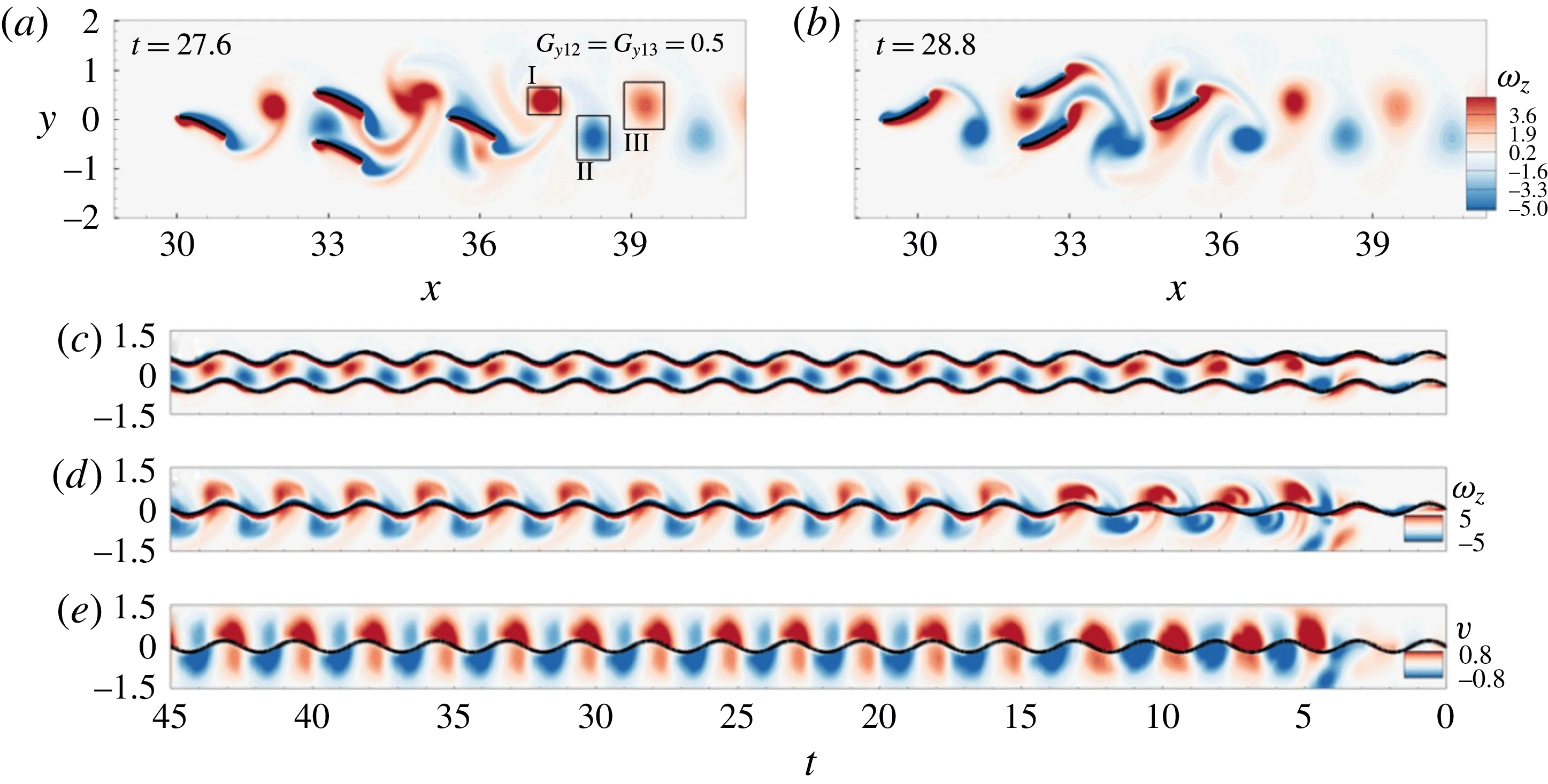
) and reveals that the positive and negative vortices shed from the trailing edges of F2 and F3 are encountered by F4 and broken into two parts in a manner similar to that of the vortex interactions observed in the stable tandem configuration. A reverse Kármán vortex street is evident in their wake. Figure 28(c) shows F2 and F3 encountering the vortices oncoming from F1. The leading edges of F2 and F3 pass over the lower and upper parts, respectively, of the oncoming vortex structures. The leading edge trajectory of F4 passes through the oncoming vortices in figure 28(d). Figure 28(e) shows the time evolution of the
 $y$
-velocity along the vertical line at the leading edge of F4 and indicates that the trajectory and the induced flows are in phase in the spanwise direction for the vortex interception mode. The spanwise-induced flows near F4 in the diamond configuration are stronger than those near F2 in the tandem configuration (figure 10
c). Table 2 shows the circulations of vortices I and II in various schooling formations at
 $t=27.6$
. A reverse Kármán vortex street is evident in the wake of the two tandem fins, and the vortex circulations are similar to those of IS. The circulation of positive vortex I increases in the diagonal configuration, where the vortex structures are deflected downwards. In the triangular configuration, the circulation is higher due to the merging process. However, the circulation decreases to the level of IS in the diamond configuration due to the vortex–body interaction with the fourth fin (F4).
(a,b) Instantaneous vorticity fields for four fins in the diamond configuration (
 $G_{y12}=G_{y13}=0.5$
) at
 $t=27.6$
and 28.8. Time evolutions of the vorticities along the vertical line at the leading edge of (c) F2 and (d) F4 in the diamond configuration. (e) Time evolution of the spanwise velocity along the vertical line at the leading edge of F4.
 $A_{f1}=A_{f2}=A_{f3}=A_{f4}=0.4$
.

(a) Input power and (b) efficiency in the diamond configuration.

Circulations of vortices I and II in various schooling configurations at
 $t=27.6$
at
 $Re=100$
.

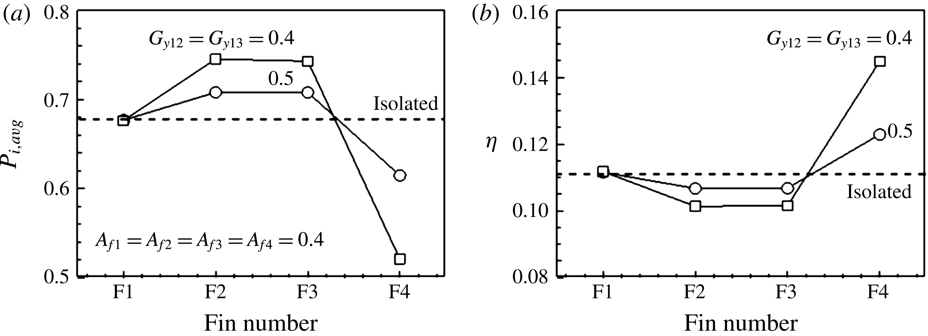
Figure 29 shows the effects of local position on swimming performance for various spanwise gap distances. The swimming velocity is the same regardless of the local position, whereas the input power and the efficiency vary in figure 29(a,b). The input powers of F2 and F3 are higher than that of IS, and decrease as the gap distance
 $G_{y}$
increases. F4 benefits from swimming through the vortex cores in the third row and the input power is reduced by 9 % and 23 % at
 $G_{y12}=G_{y13}=0.5$
and 0.4, respectively. The efficiency of F4 is enhanced due to the decrease in the input power, and increases as the spanwise gap distance decreases. There is a trade-off between the required input powers of the fins in the second and third rows. F2 and F3 can modulate the spanwise gap distance to minimize the penalty of the increased input power, which offsets the advantage of the decreased input power of F4. The global efficiencies of the fins at
 $G_{y}=0.4$
and 0.5 are 0.113 and 0.111, respectively.
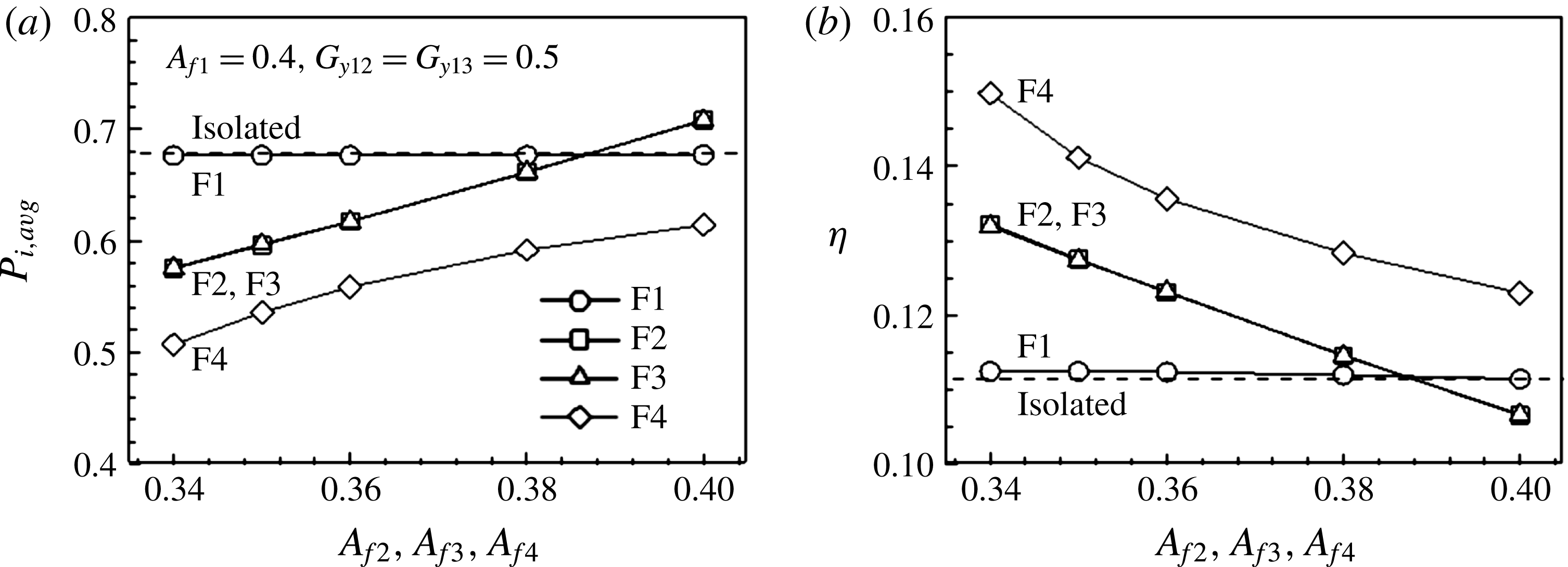
The reduced heaving amplitudes of the trailing fins play an important role in decreasing their input power for the diagonal and triangular configurations. The stable diamond configuration forms spontaneously despite the reduced heaving amplitudes of F2, F3 and F4. Figure 30 shows the variation in swimming performance with the heaving amplitude. The heaving amplitudes of F2, F3 and F4 are the same. The swimming speed of the school remains constant as the heaving amplitudes of F2, F3 and F4 decrease, as was the case for IS. The input powers of F2 and F3 are less than that of IS because of the decreased heaving amplitude, and F4 can reduce its input power by approximately 26 % at
 $A_{f4}=0.34$
in figure 30(a). Figure 30(b) indicates that the individual efficiencies are enhanced by 22 % for F2 and F3 and by 36 % for F4 relative to that of the leading fin F1 due to the reduced heaving amplitudes
 $A_{f2}=A_{f3}=A_{f4}=0.34$
.
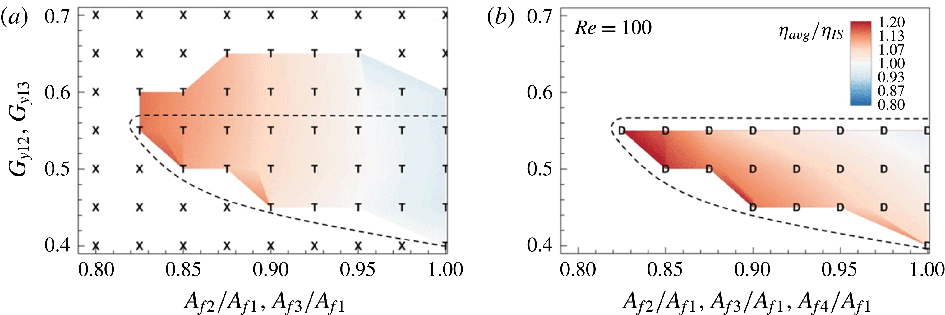
In the present system, both the spanwise gap distance and the heaving amplitude of the trailing fins (F2, F3 and F4) are the main factors in determining whether stable configurations are formed or not. Figure 31 shows the phase diagram for the parameter space spanned by the normalized heaving amplitudes (
 $A_{f2}/A_{f1}$
,
 $A_{f3}/A_{f1}$
,
 $A_{f4}/A_{f1}$
) and the spanwise gap distances (
 $G_{y12}$
,
 $G_{y13}$
) for the triangular and diamond configurations at
 $Re=100$
. ‘X’ denotes unstable schoolings and ‘T’ and ‘D’ denote the stable triangular and diamond configurations, respectively. The contours show the average efficiencies of the members (
 $\unicode[STIX]{x1D702}_{avg}$
) normalized by that of IS (
 $\unicode[STIX]{x1D702}_{IS}$
). Figure 31(a) shows that spanwise gap distances that are too large or too small prevent the formation of the stable triangular configuration for three fins. The average efficiency is affected more by the heaving amplitude of the fins swimming in the second column than by the spanwise gap distance, and increases as the amplitude decreases. The area in the parametric space of the stable diamond configuration enclosed by the dashed line decreases upon the addition of one individual into the wake of the triangular configuration. The average efficiency increases as the heaving amplitude and the spanwise gap distance decrease. The average efficiency is enhanced by 14 % and 19 % over that of IS in the stable triangular and diamond configurations, respectively, by diminishing the heaving amplitude of F2, F3 and F4.
(a) Input power and (b) efficiency as a function of the heaving amplitude of F2, F3 and F4 in the diamond configuration.

Phase diagram spanned by the normalized heaving amplitudes (
 $A_{f2}/A_{f1}$
,
 $A_{f3}/A_{f1}$
,
 $A_{f4}/A_{f1}$
) and the spanwise gap distances (
 $G_{y12}$
,
 $G_{y13}$
) for the (a) triangular and (b) diamond configurations at
 $Re=100$
. ‘
 $\mathsf{X}$
’ denotes the unstable schoolings and ‘
 $\mathsf{T}$
’ and ‘
 $\mathsf{D}$
’ denote the stable triangular and diamond configurations respectively. The contours show the average efficiencies of the members (
 $\unicode[STIX]{x1D702}_{avg}$
) normalized by
 $\unicode[STIX]{x1D702}_{IS}$
. The dashed line denotes the boundary of the stable region for the diamond configuration.

3.7 Effects of Reynolds number on the stable configurations
Figure 32 displays the time histories of the gap distances
 $G_{x12}$
,
 $G_{x13}$
and
 $G_{x14}$
in the diamond configuration at
 $Re=100$
, 800 and 1200. The four fins with an identical heaving motion at their leading edges (
 $A_{f}=0.4$
) form the stable diamond configuration at
 $G_{y12}=G_{y13}=0.4$
. The streamwise gap distances between the fins swimming in the first, second and third columns increase as the Reynolds number increases from 100 to 800 or 1200. Figure 33 shows the phase diagram spanned by the normalized heaving amplitudes (
 $A_{f2}/A_{f1}$
,
 $A_{f3}/A_{f1}$
,
 $A_{f4}/A_{f1}$
) and the spanwise gap distances (
 $G_{y12}$
,
 $G_{y13}$
) in the (a) triangular and (b) diamond configurations at
 $Re=1200$
. The regions for the stable configuration are slightly reduced as Re increases, and the regions that become unstable at high Re correspond to those of the least efficient cases at low Re in figures 31 and 33. The contours exhibit the average efficiency (
 $\unicode[STIX]{x1D702}_{avg}$
) normalized by
 $\unicode[STIX]{x1D702}_{IS}$
. At
 $Re=100$
, F2 and F3 propelled with the same heaving amplitude of the leading edge as that of F1 required a greater input power in the triangular and diamond stable configurations due to the high-pressure region created in the lower part of F2 and upper part of F3 during the downstroke and upstroke, respectively. The penalty of the increased input power is attenuated as the transverse distance between F2 and F3 increases, but the average efficiency is still lower than
 $\unicode[STIX]{x1D702}_{IS}$
regarding the same heaving amplitude in figure 31. The reduced heaving amplitude for the fins located in the second column is mandatory to save energy by schooling in the triangular and diamond configurations at
 $Re=100$
. As Re increases, the viscous effect becomes less important and the penalty caused by the transverse proximity of F2 and F3 is mitigated. At
 $Re=1200$
, the global efficiency in the triangular configuration slightly increases over
 $\unicode[STIX]{x1D702}_{IS}$
when the heaving amplitudes are the same, and increases by up to 19 % by reducing the heaving amplitudes of F2 and F3. F2 and F3 can keep pace with F1 with reduced heaving amplitudes by 17.5 %, and the global efficiency increases by 33 %.
Time histories of the gap distances
 $G_{x12}$
,
 $G_{x13}$
and
 $G_{x14}$
for different Reynolds numbers in the diamond configuration. The black, red and blue lines denote
 $Re=100$
, 800 and 1200, respectively.

Phase diagram spanned by the normalized heaving amplitudes (
 $A_{f2}/A_{f1}$
,
 $A_{f3}/A_{f1}$
,
 $A_{f4}/A_{f1}$
) and the spanwise gap distances (
 $G_{y12}$
,
 $G_{y13}$
) in the (a) triangular and (b) diamond configurations at
 $Re=1200$
. ‘
 $\mathsf{X}$
’ denotes the unstable schoolings and ‘
 $\mathsf{T}$
’ and ‘
 $\mathsf{D}$
’ denote the stable triangular and diamond configurations, respectively. The contours show the average efficiency (
 $\unicode[STIX]{x1D702}_{avg}$
) normalized by
 $\unicode[STIX]{x1D702}_{IS}$
. The dashed line denotes the boundary of the stable region for the diamond configuration.

Schematic diagram of the swimming flexible fin in the midst of the downstroke. The fin moves from the black line to the blue line over
 $\unicode[STIX]{x0394}t$
.

The triangular and diamond configurations can be achieved with the reduced heaving amplitudes imposed on the leading edges of F2, F3 and F4, which results in the decreased input power required to swim at the same velocity as that of F1. The input powers of the fins located in the second and third columns are reduced by the vortex–vortex and vortex–flexible body interactions as well as by the reduced flapping motions. We used the reactive model of Lighthill (Reference Lighthill1960) to examine the benefit of the reduced input power from the hydrodynamic interactions. The scaling approximation based on the reactive model was employed for the flexible fin to explore the effects of swimming near the ground (Park, Kim & Sung Reference Park, Kim and Sung2017). The fin transfers energy to the fluid by its undulating body motion, and the energy of the fluid is consumed in two ways: (i) pushing the fin forwards and (ii) creating wakes behind the fin (Lighthill Reference Lighthill1960). Figure 34 shows a schematic diagram of the swimming flexible fin, which moves horizontally and transversely over
 $\unicode[STIX]{x0394}t$
. During
 $\unicode[STIX]{x0394}t$
, the fin moves horizontally (
 $\unicode[STIX]{x0394}tU_{c}$
) and transversely (
 $\unicode[STIX]{x0394}tV_{t}$
), where
 $V_{t}$
is the transverse velocity of the trailing edge. The surrounding fluid is pushed over a distance (
 $\unicode[STIX]{x0394}tV_{e}$
), where
 $V_{e}$
is the effective transverse velocity (Lighthill Reference Lighthill1960; Lauder & Tytell Reference Lauder and Tytell2005). The effective transverse velocity
 $V_{e}$
was derived by examining two similar triangles in figure 34,
 $$\begin{eqnarray}\displaystyle & \displaystyle V_{e}=V_{t}\left(1-\frac{\unicode[STIX]{x0394}tU_{c}}{L\cos \unicode[STIX]{x1D703}}\right). & \displaystyle\end{eqnarray}$$
The fin increases the transverse momentum of the fluid by
 ${\sim}V_{e}$
. The fin does work at a rate
 ${\sim}V_{t}$
as it moves transversely, and the transverse momentum is shed into the wake at the same rate that the fin moves horizontally
 ${\sim}U_{c}$
(Lighthill Reference Lighthill1960; Lauder & Tytell Reference Lauder and Tytell2005). The input power during one flapping period is then proportional to
 $P_{i,avg}\sim \bar{V}_{e}U_{avg}\bar{V}_{t}$
, where
 $\bar{V}_{e}$
and
 $\bar{V}_{t}$
are the time-averaged effective velocity and transverse velocity, respectively. The time-averaged effective velocity and the input power are proportional to
 $$\begin{eqnarray}\displaystyle & \displaystyle \bar{V}_{e}\sim \bar{V}_{t}\left(1-\frac{\tan \bar{\unicode[STIX]{x1D703}}}{St}\right), & \displaystyle\end{eqnarray}$$
 $$\begin{eqnarray}\displaystyle & \displaystyle P_{i,avg}\sim U_{avg}\bar{V}_{t}^{2}\left(1-\frac{\tan \bar{\unicode[STIX]{x1D703}}}{St}\right), & \displaystyle\end{eqnarray}$$
where
 $\bar{\unicode[STIX]{x1D703}}$
is the average absolute value of the deflection angle and St is the Strouhal number
 $St=f_{f}A_{trailing}/U_{avg}=\bar{V}_{t}/U_{avg}$
.
In the stable configurations, the trailing fins reduced the input power not only by the flow-meditated interaction among the fins but also by decreasing the heaving amplitude as compared to the leading fin. In figure 35, the average input power
 $P_{avg}$
is plotted as a function of (3.7) to figure out how much the fins benefitted solely from the flow-mediated interactions according to their local positions. The benefit of the reduced input power by decreasing the heaving amplitude was reflected in (3.7). The symbols in black, red and blue denote the fins swimming in the first (F1), second (F2 and F3) and third columns (F4), respectively. The slope was determined by minimizing the squared residuals for each group (figure 35). The input powers of the fins located in the second (F2 and F3) and the third columns (F4) in the finite diamond formation are reduced approximately by 24 % and 40 % relative to that of the leading fin, respectively, as a pure result of the hydrodynamic interactions. The data set obtained at
 $Re=100$
deviated slightly from the average trend (dashed line) of higher Reynolds numbers. The input powers of F2 and F3 at
 $Re=100$
(red circle symbols in figure 35) were generally larger than the average trend, which was consistent with the results in figures 31 and 33; the penalty of the increased input power to F2 and F3 was diminished as Re increased.
Time-averaged input power. The circle, square, triangle and diamond symbols denote
 $Re=100$
, 400, 800 and 1200, respectively. The symbols in black, red and blue denote the fins swimming in the first, second and third columns, respectively. The slope is determined by minimizing the squared residuals for each group.

The energetic benefits of schooling for individual fish depend on their local positions. Synchronized swimming in a rectangular pattern has hydrodynamic advantages for individuals, which can swim 20 % faster than a solitary individual with a similar amount of energy because of the channelling effect (Daghooghi & Borazjani Reference Daghooghi and Borazjani2015). Hemelrijk et al. (Reference Hemelrijk, Reid, Hildenbrandt and Paddling2015) found that fish in four different configurations (diamond, rectangular, phalanx and line) always swim more efficiently than a lone fish, and the efficiency of the diamond configuration is enhanced by approximately 23 %. Periodic boundary conditions were imposed to model an infinite school of fish in which the individuals swim within a predetermined schooling structure (Daghooghi & Borazjani Reference Daghooghi and Borazjani2015; Hemelrijk et al. Reference Hemelrijk, Reid, Hildenbrandt and Paddling2015). It is difficult to extract the dependence of the hydrodynamic advantages of fish schooling on local positioning for an infinite school. In the present study, the size of the school was finite, and the individuals actively coordinated their movements in the horizontal direction and were found to form four basic stable configurations, i.e. tandem, diagonal, triangular and diamond configurations. Two self-propelled swimmers cannot sustain their tandem configuration with an a priori specified body deformation, and the follower equipped with a reinforcement learning ability can maintain its position relative to the leader (Novati et al. Reference Novati, Verma, Alexeev, Rossinelli, Rees and Koumoutsakos2017). Swimming in a sustained tandem formation provides the follower with a 30 % reduction in energy expenditure. While this reduced energy of the follower in the tandem configuration was consistent with the finding of Novati et al. (Reference Novati, Verma, Alexeev, Rossinelli, Rees and Koumoutsakos2017), the mechanism for realizing the stable configurations was different due to different body characteristics of the swimmers. The swimmer in Novati et al. (Reference Novati, Verma, Alexeev, Rossinelli, Rees and Koumoutsakos2017) had a finite thickness body and was free to move in both the transverse and horizontal directions. The present fin was constrained in the transverse direction due to the imposed heaving motion at the leading edge, and free to move in the horizontal direction. The flexibility of the fin was considered here, and the undulations of the other parts besides the leading edge were adjusted according to the fluid–flexible-body interaction.
The triangular and diamond schooling configurations can be sustained purely by hydrodynamic interactions, as is the case for the tandem and diagonal configurations. The individual group members leave behind distinctive hydrodynamic footprints. As the number of group members increases, the vortex interactions become more complex, but the flow fields in their wake are observed to converge. The wake features of the stable tandem, triangular and diamond configurations contain reverse Kármán vortex streets, which suggests the possibility of stable configurations that form spontaneously even for much larger populations. Furthermore, the observed hydrodynamic mechanisms of the basic configurations are potentially relevant to larger schools.
4 Conclusions
In this paper, we investigated the vortex–vortex and vortex–flexible-body interactions of flexible fins propelled in four stable configurations, i.e. tandem, diagonal, triangular and diamond, and explored the hydrodynamic advantages of these schooling behaviours. The flexible fin was imposed by the transverse heaving motion at the leading edge, and not constrained in the horizontal direction. The fins adjusted their relative positions in the horizontal direction dynamically. In the present system, the main factors in determining the stable configuration were the spanwise gap distance and the heaving amplitude. For the tandem configuration (
 $G_{y12}=0$
), the relative positions between the two fins are determined dynamically, and only discrete values are attainable. The trailing edge amplitude of F2 increases when it encounters oncoming vortices, which leads F2 to follow F1 despite passing through the jet-like core region formed in the wake of F1. The following fin F2 passes through the cores of the oncoming vortices in the stable tandem configuration, i.e. in the vortex interception mode, which allows F2 to reduce the input power as compared to that of F1. The leading edge motions of F2 and the flows induced by the oncoming vortices are synchronized in the spanwise direction in the vortex interception mode, which leads to a reduction in the input power by up to 14 % for the same heaving amplitudes of F1 and F2. F2 is more likely to pass through the negative u-velocity region created in the wake of F1 by swimming with a spanwise offset than without an offset. The stable diagonal configurations form due to the purely hydrodynamic interactions within the spanwise gap distance 0
 ${<}G_{y12}<0.8$
. When the spanwise gap increases above 0.8, the diagonal configuration becomes unstable and active adaptations of body motions would be required for sustained schooling. F2 swimming with
 $G_{y12}>1$
benefits from the flows induced in the swimming direction and catches up with F1 to produce the side-by-side configuration. In the stable diagonal configuration, the leading edge trajectory of F2 passes over the lower parts of the oncoming vortices at
 $G_{y12}=0.5$
, which leads to a decrease in the benefits directly induced from hydrodynamic interactions, i.e. only a 6 % reduction in the input power is achieved for F2 with respect to that of F1 for the same heaving amplitude. F2 can follow F1 and form the stable diagonal formation (
 $G_{y12}=0.5$
) even with the reduced heaving amplitude by 15 % as compared to that of F1, where the individual efficiency of F2 is increased by up to 26 % (
 $A_{f2}=0.34$
).
The oncoming vortices shed from F1 separate into two parts when they encounter F2 swimming directly behind F1. In contrast, both the positive and the negative oncoming vortices merge into those generated by the downstrokes and upstrokes of the F2 trailing edge, which strengthens the vorticities. The downstream movement of the positive vortices is delayed by the merging process, which breaks the symmetric wake structures. The deflected vortex structures induce streamwise flows in the swimming direction near the core region, which helps F3 catch up to the leading fins and form another stable configuration, i.e. the triangular configuration. The constraints on stable schooling configurations induced purely by hydrodynamic interactions become severe as the number of members increases. Spanwise gap distances that are too small or too large prevent the three fins from swimming in self-sustained triangular configurations; the stable triangular configurations are formed for
 $0.4\leqslant G_{y12}(=G_{y13})\leqslant 0.6$
if the heaving amplitudes of F1, F2 and F3 are the same. F2 and F3 are not able to keep pace with F1 when the spanwise gap distance is too small, and they catch up with the leader to form side-by-side configurations when the distance is too large. For the same heaving amplitudes of the fins propelled in the stable triangular configurations at
 $Re=100$
, F2 and F3 require more input power (5 %) than F1 to swim at the same speed because of the significantly higher pressure regions outside of the second-row fins. The input power required for the flapping motion is reduced as the heaving amplitude of the leading edge decreases. The fins swimming in the second row (F2 and F3) need to diminish their heaving amplitudes to ensure the hydrodynamic benefits from swimming behind the leading fin, and their input powers decrease by 15 % relative to that of F1 at
 $A_{f2}=A_{f3}=0.34$
.
The number of vortices does not increase linearly with increases in the number of members in a group, due to the vortex–vortex and vortex–body interactions. The wake structures of the stable triangular configurations feature a reverse Kármán vortex street consisting of one pair of alternating positive and negative vortices, which are the merged forms of the vortices generated by F1, F2 and F3. The vorticity value of each vortex increases due to the merging process, which helps F4 to further decrease its required input power by swimming in the wake of the three triangular leading fins. The range of spanwise gap distances for the stable diamond configuration is slightly reduced in comparison to that for the triangular configuration, i.e.
 $0.4\leqslant G_{y12}(=G_{y13})<0.6$
. The heaving amplitude imposed on the leading edges of F2, F3 and F4 can be reduced by 17.5 % to decrease the input power while keeping a stable triangular or diamond configuration. For the triangular and diamond stable configurations at
 $Re=100$
, the optimal global efficiency obtained by swimming in a group increases by 14 % and 19 %, respectively, achieved by diminishing the heaving amplitudes of F2, F3 and F4 (
 $A_{f2}=A_{f3}=A_{f4}=0.33$
). For the same heaving amplitude, the individual efficiency of F2 and F3 decreases by 5 %, and that of F4 increases by 10 % as compared to F1. When the heaving amplitudes of F2, F3 and F4 are reduced, on the other hand, the individual efficiency is enhanced by 22 % for F2 and F3 and by 36 % for F4. The phase diagram spanned by the spanwise gap distance and normalized heaving amplitude for the stable configurations slightly decreases as Re increases. The penalty of the increased input power to the fins in the second column is attenuated, and the average efficiency increases as Re increases from 100 to 1200. The scaling approximation based on the reactive model of Lighthill (Reference Lighthill1960) was used to isolate the benefits resulting from the hydrodynamic interactions among the flexible fins. The fins swimming in the second and third columns of the finite diamond configuration could reduce their input power by approximately 24 % and 40 %, respectively, relative to that of the leading fin, purely through the flow-mediated interactions among the fins. Our investigations of the mechanisms by which the fins swimming in basic configurations interact with each other via their shared fluid environment should provide significant insights into how fish in a school benefit hydrodynamically by varying their local positions.
Acknowledgements
This study was supported by the Creative Research Initiatives (No. 2017-013369) programme of the National Research Foundation of Korea (MSIP).
Supplementary movies
Supplementary movies are available at https://doi.org/10.1017/jfm.2018.64.