1. Introduction
Due to the rapid development of science and technology in recent years, awareness of environmental issues such as shortage in energy resources has increased substantially. To solve these environmental problems, it is extremely important to improve the energy efficiency of industrial machinery by reducing flow drag. Flow drag is classified into pressure and friction drag. Shape optimisations for reduction of the pressure drag have already been put into practice, e.g. the optimisation of the nose shape of bullet trains. On the other hand, most control methods for friction drag reduction have not yet been in practical use, except for the successful case of polymer additive in a pipeline (White & Mungal Reference White and Mungal2008). However, since friction drag is often dominant in many industrial applications (Gad-el Hak Reference Gad-el Hak1994), there is a strong need to develop an effective method to reduce friction drag.
Flow control methods can be classified into passive and active control methods. Although the implementation of passive control, e.g. riblets (Walsh Reference Walsh1983) and polymer additives (White & Mungal Reference White and Mungal2008), is relatively easier because only the initial processing is required, the high additional maintenance cost beyond the drag reduction effect makes its implementation challenging. On the other hand, active control methods have attracted much attention in recent years despite the need for energy input from the external system, because both numerical simulations and experiments have shown significant drag reduction effects, such as relaminarisation of the flow field and sub-laminar drag. As the simplest active control method, the controls of using blowing and suction from the wall have been widely investigated. Therefore, in the present work, we focus only on active control methods by using blowing and suction.
The active control methods can be further classified into predetermined and feedback control methods. In the predetermined control methods (e.g. Ricco et al. Reference Ricco, Skote and Leschziner2021; Fukagata et al. Reference Fukagata, Iwamoto and Hasegawa2024), we impose the control input predetermined independently of the flow field. Among the predetermined control methods, uniform blowing/suction (UB/US) is the simplest predetermined control method, in which a uniform wall-normal velocity is imposed on the wall. Sumitani & Kasagi (Reference Sumitani and Kasagi1995) performed direct numerical simulations (DNS) of a relatively low Reynolds number turbulent channel flow controlled using UB/US. According to their study, the friction drag decreases on the UB side despite the increase in the turbulence intensity, and vice versa on the US side. Subsequently, a similar control effect was observed in a spatially developing turbulent boundary layer flow at low to high Reynolds numbers (Kametani & Fukagata Reference Kametani and Fukagata2011; Kametani et al. Reference Kametani, Fukagata, Örlü and Schlatter2015; Noguchi et al. Reference Noguchi, Fukagata and Tokugawa2016). Recently, this control effect has been investigated in more complicated flow fields, i.e. a turbulent plane Couette flow (Kraheberger et al. Reference Kraheberger, Hoyas and Oberlack2018; Nabae & Fukagata Reference Nabae and Fukagata2024), a supersonic turbulent channel flow (Kametani et al. Reference Kametani, Kotake, Fukagata and Tokugawa2017), and flow around an aerofoil (Eto et al. Reference Eto, Kondo, Fukagata and Tokugawa2019; Atzori et al. Reference Atzori, Vinuesa, Fahland, Stroh, Gatti, Frohnapfel and Schlatter2020; Hirokawa et al. Reference Hirokawa, Eto, Fukagata and Tokugawa2020a
,
Reference Hirokawa, Ohashi, Eto, Fukagata and Tokugawab
; Ohashi et al. Reference Ohashi, Morita, Hirokawa, Fukagata and Tokugawa2020, Reference Ohashi, Fukagata and Tokugawa2021; Miura et al. Reference Miura, Ohashi, Fukagata and Tokugawa2022). In contrast to the predetermined control, the control input in the feedback control is determined based on the state of the flow field. The simplest feedback control method is the opposition control proposed by Choi et al. (Reference Choi, Moin and Kim1994). In this control method, a detection plane parallel to the wall is placed in the flow field, and the wall-normal velocity opposite to the velocity detected on the detection plane is imposed on the walls. Choi et al. (Reference Choi, Moin and Kim1994) showed by DNS that the friction drag is reduced by up to
 $25\,\%$
in a relatively low Reynolds number turbulent channel flow. In the opposition control, quasi-streamwise vortices (QSV) in the region near the wall are suppressed, leading to the suppression of the self-regenerating cycle (Hamilton et al. Reference Hamilton, Kim and Waleffe1995; Waleffe Reference Waleffe1997) in a wall-bounded flow. Subsequently, Hammond et al. (Reference Hammond, Bewley and Moin1998) optimised the location of the detection plane in the opposition control, and the drag reduction rate was found to be maximum when the detection plane was placed approximately
 $15$
wall units above the wall. Although the drag reduction mechanism by the opposition control is opposite to that by the UB/US, both control methods are suited to investigate the effect of active control in wall turbulence.
Until now, investigations of the effects of various flow control methods have been limited mostly to basic flow fields in simple geometries, e.g. flat plates and straight ducts. On the other hand, the control effect in flow over a curved wall with a non-uniform pressure gradient has rarely been investigated due to the complexity of the flow geometry. In channel flow with a bump, the flow is separated in the region behind the bump, inducing an adverse pressure gradient. Since the flow separation behind the bump makes the flow field anisotropic and inhomogeneous, it is difficult to conduct experiments and numerical simulations in this flow field. However, investigation of the control effect on turbulent channel flow with a bump is inevitable from both engineering and theoretical viewpoints, and it is indispensable for the practical application of control methods.
Although there are a few studies even in uncontrolled flows compared with a turbulent plane channel flow, numerical simulations and experiments of channel flow with a bump have been conducted. Almeida et al. (Reference Almeida, Durao and Heitor1993) conducted experiments on turbulent flows in a channel with periodic two-dimensional bumps, and quantitatively investigated the flow over bumps. Subsequently, using the bump geometry similar to Almeida et al. (Reference Almeida, Durao and Heitor1993), DNS (Breuer et al. Reference Breuer, Peller, Rapp and Manhart2009) and large-eddy simulations (LES) (Temmerman et al. Reference Temmerman, Leschziner, Mellen and Fröhlich2003; Fröhlich et al. Reference Fröhlich, Mellen, Rodi, Temmerman and Leschziner2005) of a flow over a bump were performed to validate numerical methods and modelling. Marquillie et al. (Reference Marquillie, Ehrenstein and Laval2011) investigated the instability of the flow separation by using DNS, and showed the relationship between the vorticity or kinetic energy production and the streak dynamics. More recently, Mollicone et al. (Reference Mollicone, Battista, Gualtieri and Casciola2017) applied the different bump geometries in a wide range of the friction Reynolds number, i.e.
 $300 \leqslant {\textit {Re}}_\tau \leqslant 900$
, and unveiled the process of flow separation by investigating the budget of turbulent kinetic energy. In a flat boundary layer flow with bumps, Webster et al. (Reference Webster, DeGraaff and Eaton1996) measured the statistics experimentally. Subsequently, Wu & Squires (Reference Wu and Squires1998) attempted to reproduce the results of Webster et al. (Reference Webster, DeGraaff and Eaton1996) through LES, but it was not successful due to insufficient grid resolution.
While the dynamics and quantitative evaluation in a flow with a bump have been investigated as mentioned above, the control effect in these complicated flows has been limited to a few studies (e.g. Fournier et al. Reference Fournier, Laval, Braud and Stanislas2010; Yakeno et al. Reference Yakeno, Kawai, Nonomura and Fujii2015; Banchetti et al. Reference Banchetti, Luchini and Quadrio2020; Mollicone et al. Reference Mollicone, Battista, Gualtieri and Casciola2022). Since the flow over a bump is highly dependent on the bump geometry and the Reynolds number, we should systematically investigate the control effect in a flow with a bump for different control methods having different drag reduction mechanisms. In the recent work by Banchetti et al. (Reference Banchetti, Luchini and Quadrio2020), the effect of a bump was studied in detail using DNS. They considered the streamwise travelling wave of spanwise wall oscillation (StTW) as the control method, and they found that the presence of a bump has a non-negligible effect on the pressure drag, leading to additional
 $10\,\%$
drag reduction, which is favourable information for further investigating this kind of control method towards its practical use. The next question is whether such an effect on the pressure drag is universal for all drag reduction control methods, or dependent on the inherent drag reduction mechanism.
On the basis of this background, the objective of the present study is to investigate the effect of blowing/suction-based control in a turbulent channel flow with a bump by using DNS. We consider two representative control methods having different drag reduction mechanisms, i.e. opposition control and UB, and consider two different Reynolds numbers and bump heights. Opposition control shares the drag reduction mechanism with StTW studied by Banchetti et al. (Reference Banchetti, Luchini and Quadrio2020) in the sense that the near-wall structures are attenuated, although the detailed mechanism of attenuation is different – formation of a virtual wall and a Stokes layer, respectively. The drag reduction mechanism of UB is totally different – UB enhances turbulence, but the drag is reduced due to the mean wall-normal momentum flux (Kametani & Fukagata Reference Kametani and Fukagata2011). In fact, such a difference is known to cause a different behaviour in the boundary layer development in the region downstream of the controlled region (Stroh et al. Reference Stroh, Hasegawa, Schlatter and Frohnapfel2016). Therefore, the flow behaviour over a bump can be different depending on the control method.
The rest of this paper is organised as follows. Section 2 summarises the numerical method for the present DNS. In § 3, we investigate the effects of opposition control and UB in a turbulent channel flow with a bump. Finally, we conclude the present study in § 4.
2. The DNS
2.1. Governing equations
The governing equations are the incompressible continuity and Navier–Stokes equations, i.e.
 \begin{align} &\qquad\qquad\qquad\qquad\quad \frac {\partial u_i}{\partial x_i} = 0, \end{align}
 \begin{align} &\frac {\partial u_i}{\partial t} = -\frac {\partial ( u_i u_j)}{\partial x_j} - \frac {\partial p}{\partial x_i} + \frac {1}{{\textit {Re}}_b} \frac {\partial ^2 u_i}{\partial x_j\,\partial x_j} - \frac {{\rm d} P}{{\rm d} x_1} \delta _{i1}, \end{align}
where
 $u_i\ ( i=1,2,3 )$
and
 $p$
represent the velocity components and pressure, respectively. All variables are made dimensionless by twice the bulk-mean velocity
 $2U_b^*$
, the channel half-width
 $\delta ^\ast$
, and the fluid density
 $\rho ^\ast$
, where the superscript
 $\ast$
denotes dimensional quantities. The bulk Reynolds number is defined as
 ${\textit {Re}}_b = 2 U_b^\ast \delta ^\ast / \nu ^\ast$
, where
 $\nu ^\ast$
is the kinematic viscosity. Hereafter, for convenience, we interchangeably denote
 $(x_1,x_2,x_3)$
and
 $(u_1,u_2,u_3)$
by
 $(x,y,z)$
and
 $(u,v,w)$
.
To enable the simulation of a turbulent channel flow with a bump in the orthogonal coordinate system, we apply the coordinate transformation proposed by Kang & Choi (Reference Kang and Choi2000), i.e.
 \begin{align} x = \xi _1,\quad y = \xi _2(1+\eta ) + \eta _l,\quad z = \xi _3, \end{align}
where
 $\xi _1$
,
 $\xi _2$
and
 $\xi _3$
denote the streamwise, wall-normal and spanwise directions in the computational space, respectively. In addition, the wall displacement represents
 $\eta = (\eta _u - \eta _l)/2$
, with
 $\eta _u$
and
 $\eta _l$
denoting the displacements of the upper and lower walls. Similarly to Banchetti et al. (Reference Banchetti, Luchini and Quadrio2020), who studied the effect of streamwise travelling waves of spanwise velocity over a bump,
 $\eta _u$
and
 $\eta _l$
are defined as
 \begin{align} \eta _u = 0,\quad \eta _l = \alpha a \exp \left [ -\left ( \frac { \xi _1 - b }{ \gamma c } \right )^2 \right ] + \alpha a^\prime \exp \left [ -\left ( \frac { \xi _1 - b }{ \gamma c^\prime } \right )^2 \right ], \end{align}
where
 $a$
,
 $a^\prime$
,
 $c$
,
 $c^\prime$
,
 $\alpha$
and
 $\gamma$
are the parameters to determine the configuration of the bump. The bump height and width are determined by
 $\alpha$
and
 $\gamma$
, respectively. In the present study, we consider two different bump heights, while the bump width in wall units is fixed in all cases. The streamwise location of the bump is set to the centre of the channel, i.e.
 $b = L_1 /2$
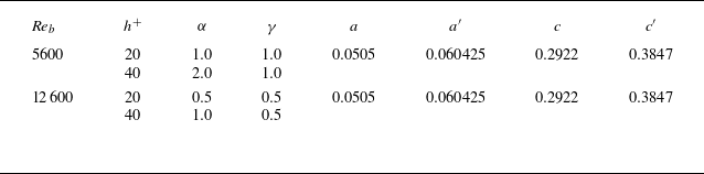
. The parameters describing the bump are summarised in table 1, where
 $h^+$
denotes the bump height, with the superscript + indicating wall units normalised by the friction velocity in the uncontrolled flow. Figure 1 shows the bump geometry in the cases with
 $h^+ \approx 20$
and
 $40$
at
 ${\textit {Re}}_b = 5600$
and
 $12\,600$
.
Parameters to determine the bump geometry.

Bump geometry in the cases with
 $h^+ \approx 20$
and
 $40$
: (a)
 ${\textit {Re}}_b = 5600$
, (b)
 ${\textit {Re}}_b = 12\,600$
. Coloured vertical lines represent the streamwise locations comparing the turbulence statistics.

By applying the coordinate transformation of (2.3), the governing equations in the boundary-fitted coordinates read
 \begin{align} &\qquad\qquad\qquad\qquad\quad \frac {\partial u_i}{\partial \xi _i} = -S_c, \end{align}
 \begin{align} &\frac {\partial u_i}{\partial t} = - \frac {\partial ( u_i u_j)}{\partial \xi _j} - \frac {\partial p}{\partial \xi _i} + \frac {1}{{\textit {Re}}_b}\frac {\partial ^2 u_i}{\partial \xi _j\,\partial \xi _j} + \frac {d P}{d \xi _1} \delta _{i1} + S_i, \end{align}
where
 $S_c$
and
 $S_i$
in (2.5) and (2.6) denote the additional terms due to the coordinate transformation, which are expressed as
 \begin{align} &\qquad\qquad\qquad\qquad\qquad S_c = \phi _j^\prime \frac {\partial u_j}{\partial \xi _2}, \end{align}
 \begin{align} S_i ={} &- \phi _j^\prime \frac {\partial ( u_i u_j)}{\partial \xi _2} - \phi _i^\prime \frac {\partial p}{\partial \xi _2} \nonumber \\ &{}+ \frac {1}{{\textit {Re}}_b} \left [ \frac {1}{2} \frac {\partial \big( \phi _j^\prime \phi _j^\prime\big)}{\partial \xi _2} \frac {\partial u_i}{\partial \xi _2} + \phi _j^\prime \phi _j^\prime \frac {\partial ^2 u_i}{\partial \xi _2^2} + 2\phi _j^\prime \frac {\partial ^2 u_i}{\partial \xi _j\, \partial \xi _2} + \frac {\partial \phi _j^\prime }{\partial \xi _j} \frac {\partial u_i}{\partial \xi _2} \right ], \end{align}
where
 \begin{align} \phi _j^\prime = \phi _j - \delta _{j2}, \end{align}
with
 \begin{align} \phi _j = \left \{ \begin{array}{ll} \displaystyle { -\frac {1}{1+\eta } \left ( \frac {\partial \eta _l}{\partial \xi _j} + \xi _2 \frac {\partial \eta }{\partial \xi _j} \right ) } & \textrm {for }j=1,3, \\ \displaystyle { \frac {1}{1+\eta } } & \textrm {for }j=2. \end{array} \right . \end{align}
The computational domain consists of two regions, i.e. a driver region without a bump, and a main region with a bump, as shown in figure 2. In the driver region, the periodic boundary condition is applied in the streamwise (
 $\xi _1$
) and spanwise (
 $\xi _3$
) directions. In the main region, we apply the inflow and outflow boundary conditions in the streamwise direction and the periodic boundary condition in the spanwise direction. The outflow boundary condition is determined by solving
 \begin{align} \frac {\partial u_i}{\partial t} + \overline {u}(y)\, \frac {\partial u_i}{\partial x} = 0, \end{align}
where
 $\overline {u}(y)$
represents the mean streamwise velocity at the downstream end of main computational domain, i.e.
 $x = L_x$
. In uncontrolled flow, the no-slip condition is applied on both walls in both driver and main regions. The velocity boundary condition on the walls in the controlled case is described in § 2.3.
Schematic of the computational domain. The opposition or UB/US controls are applied in the grey region.

2.2. Numerical schemes and conditions
The DNS code in the present study is based on that developed by Fukagata et al. (Reference Fukagata, Kasagi and Koumoutsakos2006) and that of a spatially developing turbulent boundary layer flow extended by Kametani & Fukagata (Reference Kametani and Fukagata2011). The governing equations are spatially discretised by using the energy-conserving second-order central difference scheme (Kajishima Reference Kajishima1999; Ham et al. Reference Ham, Lien and Strong2002) and temporally integrated by using the low-storage, third-order Runge–Kutta/Crank–Nicolson scheme (Spalart et al. Reference Spalart, Moser and Rogers1991).
All simulations in the present study are conducted under a constant flow rate condition at the bulk Reynolds numbers
 ${\textit {Re}}_b = 5600$
and
 $12\,600$
, which correspond to the friction Reynolds numbers
 ${\textit {Re}}_\tau \approx 180$
and
 $360$
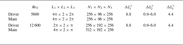
, respectively, in the uncontrolled flow. The computational conditions are shown in table 2, where
 $L_i$
,
 $N_i$
and
 $\Delta \xi _i$
denote the length of the computational domain, the number of grid points, and the grid width, respectively, in the
 $i$
th direction. The turbulence statistics presented in § 3 are computed using
 $20\,000$
instantaneous fields collected in the period
 $T^+_{{period}} = 3000$
. We have confirmed from a comparison with some representative statistics computed with
 $T^+_{{period}} = 6000$
that
 $T^+_{ {period}} = 3000$
is sufficient to discuss the effect of the bump on the turbulence statistics.
Computational conditions.

2.3. Control laws
In the present study, we consider two representative control methods: opposition control (Choi et al. Reference Choi, Moin and Kim1994; Hammond et al. Reference Hammond, Bewley and Moin1998) and UB (Sumitani & Kasagi Reference Sumitani and Kasagi1995; Kametani & Fukagata Reference Kametani and Fukagata2011). For both cases, the control input is applied in both driver and main regions so that the controlled flow is fully developed already at the inlet of the main region.
For the opposition control, the velocity on the lower wall (
 $\xi _2 = 0$
) is imposed as
 \begin{align} v \left ( \xi _1,0,\xi _3 \right ) = - \left [ v (\xi _1,\xi _{2,d},\xi _3) - \overline {v (\xi _1,\xi _{2,d},\xi _3)}^{\xi _3} \right ], \end{align}
where
 $\xi _{2,d}$
denotes the location of the detection plane. Note that the second term on the right-hand side in (2.12) is added to make the total mass flux from the wall zero. Similarly to the lower wall, we impose the wall-normal velocity on the upper wall by using the wall-normal velocity in the plane at distance
 $\xi _{2,d}^+$
from the upper wall. In this study, the detection plane is set to
 $\xi _{2,d}^+ \approx 15$
, which is the optimised location in Hammond et al. (Reference Hammond, Bewley and Moin1998).
For UB, similarly to Sumitani & Kasagi (Reference Sumitani and Kasagi1995), a constant wall-normal velocity is imposed on the lower wall with a bump, while the same amount of US is applied on the upper flat wall to keep the mass flow rate, i.e.
 \begin{align} v \left ( \xi _1,0,\xi _3 \right ) = v \left ( \xi _1,2,\xi _3 \right ) = V_w = A U_b, \end{align}
where
 $A$
is the amplitude of UB/US. In this study,
 $A$
is set to
 $0.1\,\%$
and
 $0.5\,\%$
of the bulk-mean velocity
 $U_b$
.
2.4. Drag coefficients and drag reduction rate
The total drag coefficient
 $C_D$
can be decomposed into the friction drag
 $C_{Df}$
and the pressure drag
 $C_{Dp}$
, i.e.
 \begin{align} C_D = C_{Df,u}+C_{Df,l}+C_{Dp,l}, \end{align}
where
 $(\cdot )_{u}$
and
 $(\cdot )_{l}$
denote quantities on the upper and lower walls, respectively. These drag coefficients are defined based on the area of the curved surface, and computed from the viscous stress tensor and the pressure on the walls similarly to Mori et al. (Reference Mori, Quadrio and Fukagata2017), who performed DNS of a flow in a channel with a wavy wall. The effect of bump height on the componential drag coefficients in the uncontrolled flow is summarised in Appendix A .
The drag reduction rate
 $R_D$
is defined as
 \begin{align} R_D = 1 - \frac {C_{D,C}}{C_{D,0}}, \end{align}
where
 $(\cdot )_0$
and
 $(\cdot )_C$
denote the values of the uncontrolled and controlled flows, respectively. Similarly to (2.15), we can define the reduction rates for the friction and pressure drag components
 $R_f$
and
 $R_p$
.
2.5. Verification
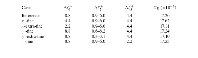
Verification for the DNS of a turbulent channel flow with a bump is performed with five different combinations of grid resolutions in table 3. Figure 3(a) compares the time history of the total drag coefficient in five different grid resolution cases. The error of
 $C_D$
in the finer cases relative to that in the the reference case is less than
 $3.2\,\%$
. Although we observe a difference in the mean wall-normal velocity at the top of the bump (red line), figures 3(b,d) and 3(c,e) show that the effect of grid resolution on the profiles of mean streamwise and wall-normal velocities is relatively small. Therefore, the grid resolution in the reference case, i.e.
 $(\Delta \xi _1^+,\Delta \xi _2^+,\Delta \xi _3) = (8.8,0.9{-}6.0,4.4)$
, is judged sufficient for investigating the effect of the bump on the drag reduction.
Computational conditions for the verification.

(a) Time history of the drag coefficient, (b,d) mean streamwise velocity, and (c,e) mean wall-normal velocity. Profiles at four different streamwise locations shown in figure 1: (b,c) solid for reference, dashed for
 $x$
-fine, dotted for
 $x$
-extra-fine; (d,e) solid for reference; dashed for
 $y$
-fine, dotted for
 $y$
-extra-fine, dash-dotted for
 $z$
-fine. The bump height is
 $h^+ \approx 20$
, and the bulk Reynolds number is
 ${\textit {Re}}_b = 5600$
.

3. Results and discussion
3.1. Opposition control
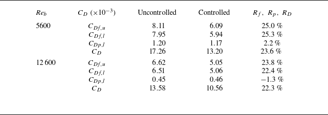
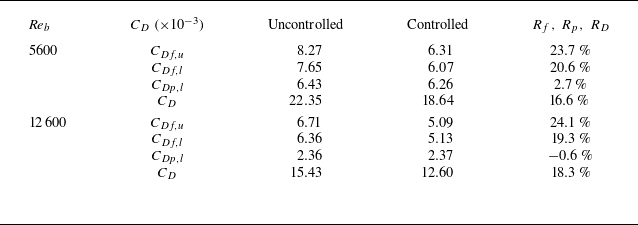
Table 4 shows the componential and total drag coefficients and the corresponding reduction rates by the opposition control in the case with a bump of height
 $h^+ \approx 20$
. The total drag
 $C_D$
can be reduced by more than
 $20\,\%$
at
 ${\textit {Re}}_b = 5600$
and
 $12\,600$
. Focusing on the drag coefficients on the lower wall at
 ${\textit {Re}}_b = 5600$
, the reduction rate of the friction drag is more than
 $25\,\%$
, while the pressure drag is only slightly decreased, i.e. reduction rate
 $2.2\,\%$
. The friction drag reduction rate in the present study is almost the same as that in the case without a bump, i.e.
 $25\,\%$
(Hammond et al. Reference Hammond, Bewley and Moin1998), on both walls. This shows that the existence of a bump hardly decreases the friction drag reduction effect, and the friction drag reduction contributes mainly to the total drag reduction even in the case with a bump. At
 ${\textit {Re}}_b = 12\,600$
, the total drag reduction rate is slightly smaller than that at
 ${\textit {Re}}_b = 5600$
. The friction drag reduction rate on the upper wall (without a bump) decreases as the Reynolds number increases. According to Chang et al. (Reference Chang, Collis and Ramakrishnan2002), in the case without a bump, the friction drag reduction rate by the opposition control mildly decreases as the Reynolds number increases. We can observe a similar trend on not only the upper wall (without a bump) but also the lower wall (with a bump). Therefore, in the case with a lower bump (i.e.
 $h^+ \approx 20$
), the effect of a bump for the opposition control effect is relatively small. As a modified version of the opposition control, we apply the opposition control to only the region where the friction coefficient on the lower wall is positive; the control is turned off in the recirculation region where the friction coefficient on the lower wall is negative. As a result, the total reduction rate in the modified opposition-controlled case is smaller than that in the original case (see Appendix B for details).
Componential drag coefficients in the uncontrolled and opposition-controlled cases, and the corresponding reduction rates in the case with bump height
 $h^+ \approx 20$
.

Visualisation of the flow fields in the uncontrolled and opposition-controlled cases at
 ${\textit {Re}}_b = 5600$
and
 $h^+ \approx 20$
: (a–d) lower wall side (with a bump); (e–h) upper wall side (without a bump). Plots for (a,b,e,f) vortical structures identified by
 $Q$
-criterion (threshold
 $Q^+ = 0.03$
), and (c,d,g,h) streak structures (i.e. streamwise velocity fluctuations
 $u^\prime$
) in the regions near the lower wall (
 $\xi _2^+ \approx 8$
) and upper wall (
 $\xi _2^+ \approx 352$
), in (a,c,e,g) the uncontrolled case, (b,d,f,h) the opposition-controlled case. Colour in (a,b,e,f) represents the wall-normal location in the physical space,
 $y^+$
.

Figure 4 shows the visualisation of the flow fields in the uncontrolled and opposition-controlled cases at
 ${\textit {Re}}_b = 5600$
and
 $h^+ \approx 20$
. Focusing on the lower wall side with a bump (figures 4
a–d), in the upstream region of the bump (
 $x^+ \lt 1000$
), QSV identified by the
 $Q$
-criterion (Hunt et al. Reference Hunt, Wray and Moin1988) are significantly suppressed by the control, similarly to the case without a bump (Hammond et al. Reference Hammond, Bewley and Moin1998). In contrast, QSV in the region behind the top of the bump (
 $1200 \lt x^+ \lt 1400$
) are hardly suppressed by the control. This implies that the opposition control is not effective in the region behind the bump. Similar to the case without a bump (Hammond et al. Reference Hammond, Bewley and Moin1998), the streak structures shown in figures 4(c,d,g,h) lined up in the spanwise direction are suppressed in the upstream and far downstream regions of the bump
 $(x^+ \lt 1000$
and
 $x^+ \gt 1400)$
. In other words, the mechanism of the friction drag reduction in the case with a bump is basically the same as that in the case without a bump. On the other hand, the streak structures in the region just behind the bump (
 $1200 \lt x^+ \lt 1400$
) are weak even in the uncontrolled case. Small velocity fluctuations in the region behind the bump lead to small control input in this region. Thus the vortical structures in the region just behind the bump remain even in the controlled case. In the region near the upper wall without a bump (figures 4
e–h), the QSV and streak structures are significantly suppressed in the controlled case. A similar modulation in the flow field was also reported in plane channel flow (Choi et al. Reference Choi, Moin and Kim1994; Hammond et al. Reference Hammond, Bewley and Moin1998), and the drag reduction rate on the upper wall (i.e.
 $25\,\%$
, as shown in table 4) is the same as that in the case of a plain channel flow at the same Reynolds number and the detection plane height (Hammond et al. Reference Hammond, Bewley and Moin1998). This implies little effect of the lower wall with a bump on the flow field in the upper wall side. This means that the interaction between the upper and lower walls on the drag reduction effect is small.
Contours of mean streamwise velocity in the uncontrolled and opposition-controlled cases at
 ${\textit {Re}}_b = 5600$
and
 $h^+ \approx 20$
: (a) uncontrolled, (b) opposition-controlled. Contour range is
 $[-3,22]$
. White lines represent zero contours.

Figure 5 shows the mean streamwise velocity in the uncontrolled and opposition-controlled cases at
 ${\textit {Re}}_b = 5600$
and
 $h^+ \approx 20$
. As shown in figure 5, streamwise velocity in the region behind the bump is negative, indicating that the flow is separated from the lower wall due to an adverse pressure gradient. In the opposition-controlled case, the reattachment point shifts further downstream, representing that flow separation is enhanced by the opposition control. The details of the control effect on the flow separation are explained in § 3.3 .
Mean streamwise and wall-normal velocities in the uncontrolled and opposition-controlled cases for
 $h^+ \approx 20$
at
 ${\textit {Re}}_b = 5600$
and
 $12\,600$
: (a,b) mean streamwise velocity; (c,d) mean wall-normal velocity. Black for upstream, red for top, green for downstream, blue for rear of the bump; dashed for uncontrolled case, solid for opposition-controlled case.

In the present study, we compare the turbulence statistics at four different locations: upstream (
 $x^+ \approx 1020$
for
 ${\textit {Re}}_b = 5600$
,
 $x^+ \approx 2150$
for
 ${\textit {Re}}_b = 12\,600$
), top (
 $x^+ \approx 1130$
for
 ${\textit {Re}}_b = 5600$
,
 $x^+ \approx 2260$
for
 ${\textit {Re}}_b = 12\,600$
), downstream (
 $x^+ \approx 1240$
for
 ${\textit {Re}}_b = 5600$
,
 $x^+ \approx 2370$
for
 ${\textit {Re}}_b = 12\,600$
) and the rear region of the bump (
 $x^+ \approx 2000$
for
 ${\textit {Re}}_b = 5600$
,
 $x^+ \approx 3130$
for
 ${\textit {Re}}_b = 12\,600$
).
Figure 6 compares the mean streamwise and wall-normal velocities,
 $U$
and
 $V$
, at four different locations. As can be observed in figures 6(a) and 6(b), the mean streamwise velocity profile in the region near the wall is slightly suppressed by the control, leading to the decrease in streamwise mean velocity gradient on the lower wall, i.e. the friction drag reduction. On the other hand, as shown in figures 6(c) and 6(d), both upward motion in front of the bump (black and red) and downward motion behind the bump (green) are suppressed by the control, which means that bump-induced motions in the region around the bump are weakened. Similar to the case without the bump (Choi et al. Reference Choi, Moin and Kim1994; Hammond et al. Reference Hammond, Bewley and Moin1998), the root mean square (RMS) of velocity fluctuations and Reynolds shear stress (RSS) in the region near the wall are suppressed by the control (see Appendix B for details). Therefore, these results imply that the decrease in turbulence intensities and friction drag suppresses bump-induced motions in the region around the bump.
Friction drag coefficient and pressure on the lower wall in the case
 $h^+ \approx 20$
at (a,b)
 ${\textit {Re}}_b = 5600$
and (c,d)
 ${\textit {Re}}_b = 12\,600$
, for (a,c) friction drag coefficient, (b,d) pressure on the lower wall. Dashed for uncontrolled case, solid for opposition-controlled case, vertical dotted for the top of the bump, horizontal dotted for
 $C_{Df,l} = 0$
or
 $p_w = 0$
.

Figure 7 shows the friction drag coefficient and pressure on the lower wall in the case
 $h^+ \approx 20$
at
 ${\textit {Re}}_b = 5600$
and
 $12\,600$
. As shown in figure 7(a), the friction drag coefficient on the lower wall is decreased by the control in the entire domain except for the region just behind the bump, in which the flow is separated. In the flow-separated region where
 $C_{Df,l} \lt 0$
(i.e.
 $1200 \lt x^+ \lt 1350$
), the friction drag coefficient is hardly decreased by the control. The region where the friction drag coefficient is reduced by the control corresponds to the region where the streak structures are weaker, as observed in figure 4. These results indicate that the effect of the friction drag reduction by the opposition control is hardly obtained in the region where the flow separation occurs. Focusing on the pressure on the lower wall shown in figure 7(b), the absolute value of
 $p_w$
is decreased by the control in the entire region. This is due to the suppression of upward motions in the upstream region and downward motions in the downstream region (figure 6
c). As shown in figures 7(c) and 7(d), we observe a similar trend at the higher Reynolds number
 ${\textit {Re}}_b = 12\,600$
.
To investigate the dependence of the bump height on the drag reduction effect, the opposition control is applied in the case where the bump height is set to be doubled, i.e.
 $h^+ \approx 40$
. The componential and total drag coefficients in the uncontrolled and opposition-controlled cases, and the corresponding reduction rates in the case with bump
 $h^+ \approx 40$
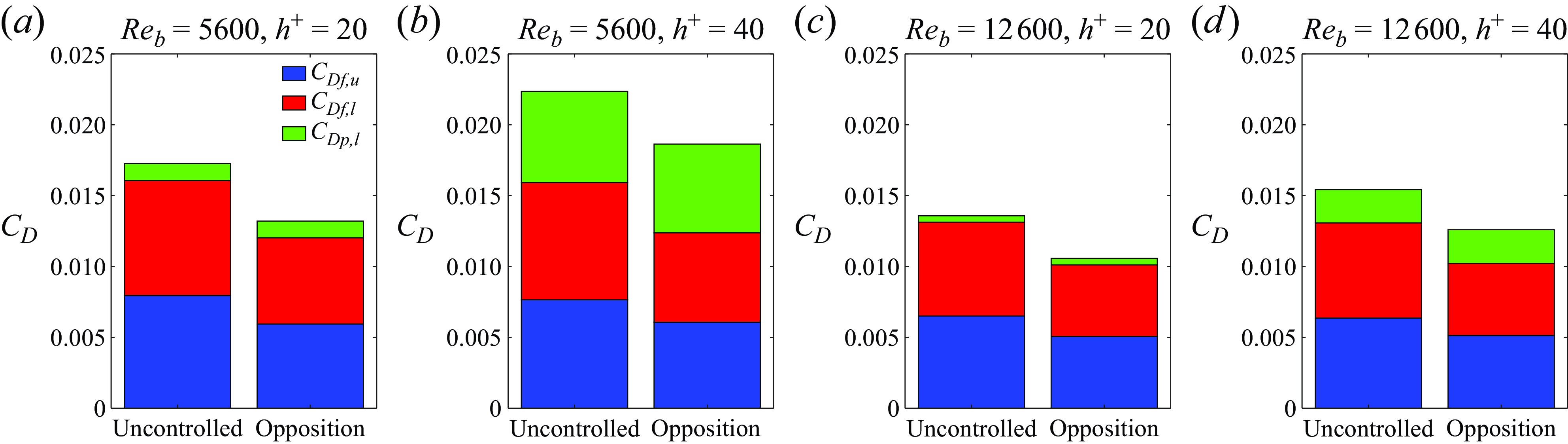
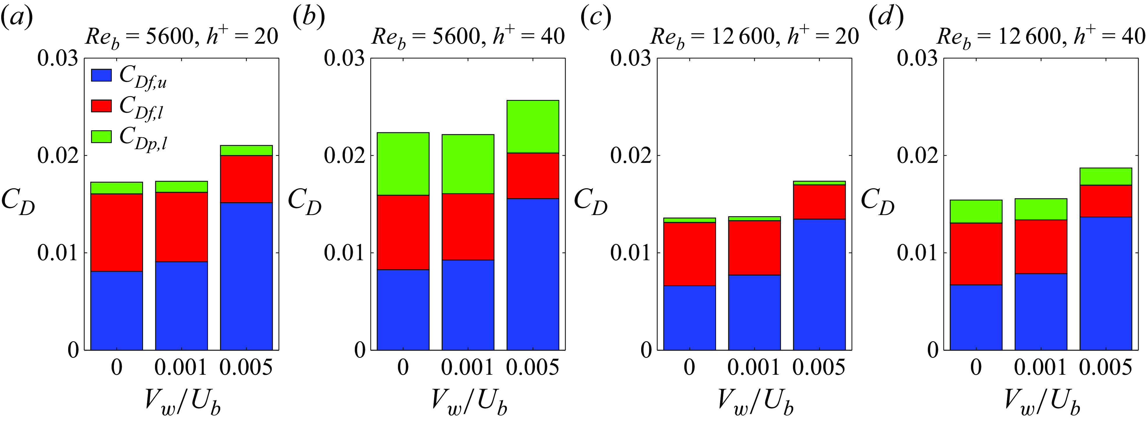
, are given in table 5, and shown graphically in figure 8. Similarly to the case
 $h^+ \approx 20$
, the friction drag is significantly decreased on both walls, while the pressure drag is nearly unchanged. However, unlike the case
 $h^+ \approx 20$
, the ratio of the pressure drag for the total drag increases as the bump height increases. Therefore, the total drag reduction rate decreases as the bump height increases.
Componential and total drag coefficients in the uncontrolled and opposition-controlled cases, and the corresponding reduction rates in the case with bump height
 $h^+ \approx 40$
.

Decomposition of drag coefficient in the uncontrolled and opposition-controlled cases: (a)
 ${\textit {Re}}_b = 5600$
,
 $h^+ \approx 20$
; (b)
 ${\textit {Re}}_b = 5600$
,
 $h^+ \approx 40$
; (c)
 ${\textit {Re}}_b = 12\,600$
,
 $h^+ \approx 20$
; (d)
 ${\textit {Re}}_b = 12\,600$
,
 $h^+ \approx 40$
.

Contours of mean streamwise velocity in the uncontrolled and opposition-controlled cases at
 ${\textit {Re}}_b = 5600$
and
 $h^+ \approx 40$
: (a) uncontrolled, (b) opposition controlled. Contour ranges is
 $[-5,22]$
. White lines represent zero contours.

Figure 9 shows the mean streamwise velocity in the uncontrolled and opposition-controlled cases at
 ${\textit {Re}} = 5600$
and
 $h^+ \approx 40$
. The trend observed in the case
 $h^+ \approx 40$
is similar to that in the case
 $h^+ \approx 20$
: the control enhances the flow separation. However, we can observe that the separated region is longer in the case
 $h^+ \approx 40$
compared with the case
 $h^+ \approx 20$
. This downstream shift of the reattachment point contributes to the increase in the pressure drag, as presented in table 5.
Friction drag coefficient and pressure on the lower wall in the case
 $h^+ \approx 40$
at (a,b)
 ${\textit {Re}}_b = 5600$
, (c,d)
 ${\textit {Re}}_b = 12600$
, for (a,c) friction drag coefficient, (b,d) pressure. Black for uncontrolled case, red for opposition-controlled case; vertical dotted for the top of the bump, horizontal dotted for
 $C_{Df,l} = 0$
or
 $p_w = 0$
.

Figure 10 shows the friction drag coefficient and pressure on the lower wall in the case
 $h^+ \approx 40$
at
 ${\textit {Re}}_b = 5600$
and
 $12\,600$
. Similar to the case
 $h^+ \approx 20$
, the friction drag is reduced in the entire domain except the separated region also in the
 $h^+ \approx 40$
case. However, the friction drag in the region behind the reattachment point (
 $x^+ \gt 1650$
) is not reduced, unlike the case
 $h^+ \approx 20$
. Although as shown in figures 10(a) and 10(c), the friction drag coefficient on the lower wall decreases as the Reynolds number increases, the trends are similar at both Reynolds numbers. Focusing on the pressure on the lower wall, regardless of the Reynolds numbers, the suppression of
 $p_w$
in the upstream region of the bump and the region near the reattachment position is clearer in the case
 $h^+ \approx 40$
, compared with the case
 $h^+ \approx 20$
.
In the opposition-controlled case, we confirm the friction drag reduction effect in the wide range except for the downstream region of the bump where the flow separation occurs. On the other hand, the opposition control has a small effect on the pressure drag or enhances the flow separation. At higher bump heights, the extension of the flow separation leads to an increase in the ratio of the pressure drag to the total drag, so that the total drag reduction rate decreases as the bump height increases. The pressure drag is slightly reduced when the bump height is small, but its effect is limited as compared to the case of StTW (Banchetti et al. Reference Banchetti, Luchini and Quadrio2020). A possible reason for the difference may be that the pressure drag reduction effect in the case of opposition control is smaller than that of StTW involving larger-scale flow modification. As for the Reynolds number dependence, the total drag reduction rate decreases as the Reynolds number increases, similar to the case without a bump (Chang et al. Reference Chang, Collis and Ramakrishnan2002).
3.2. Uniform blowing
Subsequently, we investigate the effect of UB on the lower wall with a bump. As mentioned earlier, an equal amount of US is applied on the upper flat wall to keep the mass flow rate. Therefore, the case is referred hereafter to as the UB/US case, although our main focus is on the drag reduction effect by UB.
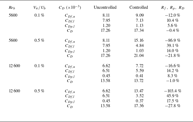
Table 6 shows the componential and total drag coefficients in the uncontrolled and UB/US cases, and the corresponding reduction rates in the case with a bump of height
 $h^+ \approx 20$
. The reduction or increase rates of each drag coefficient increase as the amplitude of UB/US increases. Similarly to the case without a bump (Sumitani & Kasagi Reference Sumitani and Kasagi1995; Kametani et al. Reference Kametani, Kotake, Fukagata and Tokugawa2017), the increase in friction drag on the US side exceeds the decrease on the UB side, leading to an increase in the total drag reduction. As for the lower wall with a bump, UB significantly reduces the friction drag, and the reduction rate of the friction drag increases as the amplitude of UB/US increases. On the other hand, unlike the opposition-controlled case, the UB/US significantly reduces the pressure drag, especially in the case of
 $0.5\,\%$
UB/US. In addition, the reduction or increase rates of the friction and pressure coefficient increase as the Reynolds number increases. The amplitude of the UB/US in wall units is represented as
 \begin{align} V_w^+ = V_w^*/u_\tau ^* = \left ( \frac {{Re}_b}{{Re}_\tau } \right ) V_w. \end{align}
Based on (3.1),
 $0.1\,\%$
of
 $U_b^+$
corresponds to
 $V^+ = 0.156$
and
 $0.0175$
at
 ${\textit {Re}}_b = 5600$
and
 $12\,600$
, respectively. In other words, the amplitude of the UB/US in wall units increases as the Reynolds number increases. Therefore, in the UB/US case, we can observe a trend on the Reynolds number opposite to that in the opposition-controlled case.
Componential and total drag coefficients in the uncontrolled and UB/US cases, and the corresponding reduction rates in the case with bump height
 $h^+ \approx 20$
.

Visualisation of vortical structures identified by the
 $Q$
-criterion (Hunt et al. Reference Hunt, Wray and Moin1988) in the uncontrolled and UB/US cases at
 ${\textit {Re}}_b = 5600$
and
 $h^+ \approx 20$
(threshold
 $Q^+ = 0.03$
): (a) uncontrolled, (b)
 $V_w/U_b = 0.1\,\%$
, (c)
 $V_w/U_b = 0.5\,\%$
. Colour represents the wall-normal location in the physical space,
 $y^+$
.

Figure 11 compares the visualisation of vortical structures identified by the
 $Q$
-criterion in the uncontrolled and UB/US cases at
 ${\textit {Re}}_b = 5600$
and
 $h^+ \approx 20$
. As can be observed in figure 11, UB enhances the vortical structures in the whole region. As explained in figure 4, in the opposition-controlled case, the control input in the flow-separated region is small due to the small turbulence intensities, whereas in the UB/US case, the control input is constant throughout the entire wall. Therefore, in the UB/US case, the UB enhances the vortical structures also in the flow-separated region.
Contours of mean streamwise velocity in the uncontrolled and
 $0.5\,\%$
UB/US cases at
 ${\textit {Re}}_b = 5600$
and
 $h^+ \approx 20$
: (a) uncontrolled, (b)
 $0.5\,\%$
UB/US. Contour ranges is
 $[-3,22]$
. White lines represent zero contours.

Figure 12 shows the mean streamwise velocity in the uncontrolled and
 $0.5\,\%$
UB/US cases at
 ${\textit {Re}}_b = 5600$
and
 $h^+ \approx 20$
. Unlike the opposition-controlled case, the reattachment point shifts upstream in the UB/US case, i.e. the suppression of the flow separation. Similarly to previous studies (Sumitani & Kasagi Reference Sumitani and Kasagi1995; Kametani & Fukagata Reference Kametani and Fukagata2011), we can observe that the turbulence intensities are enhanced by UB as shown in figure 11. Since the flow is separated due to a lack of kinetic energy to oppose the adverse pressure gradient, the increase in the turbulent kinetic energy by the UB results in the suppression of the flow separation, leading to the suppression of the pressure drag as shown in table 6.
Mean streamwise and wall-normal velocities in the uncontrolled and UB/US cases
 $h^+ \approx 20$
at
 ${\textit {Re}}_b = 5600$
and
 $12\,600$
: (a,b) mean streamwise velocity; (c,d) mean wall-normal velocity. Black for upstream, red for top, green for downstream, blue for rear of the bump; dotted for uncontrolled case, dashed for
 $0.1\,\%$
UB/US case, solid for
 $0.5\,\%$
UB/US case.

Figure 13 compares the mean streamwise and wall-normal velocities in the uncontrolled and UB/US cases
 $h^+ \approx 20$
at
 ${\textit {Re}}_b = 5600$
and
 $12\,600$
. Note that the streamwise locations where the turbulence statistics are compared, and the meanings of the line colours, are the same as those in figure 6. As observed in figures 13(a) and 13(b), the mean streamwise velocity shifts towards the suction side wall by the UB/US in all locations. This upward shift results in the reduction of the viscous shear stress, leading to the friction drag reduction on the blowing side wall. In addition, regardless of the Reynolds number, the flow separation is slightly suppressed in the downstream region of the bump (see the zoomed views in figures 13
a,b). Focusing on the mean wall-normal velocity shown in figures 13(c) and 13(d), the upward motions at the upstream position (black) and downward motions at the downstream position (green) are suppressed by the UB/US, similarly to the opposition-controlled case (figures 6
c,
d). In addition, the trends in the RMS velocity fluctuations and RSS are basically similar to those in the case without the bump (Sumitani & Kasagi Reference Sumitani and Kasagi1995; Kametani & Fukagata Reference Kametani and Fukagata2011) (see Appendix B for details).
Friction drag coefficient and pressure on the lower wall in the case
 $h^+ \approx 20$
at (a,b)
 ${\textit {Re}}_b = 5600$
, (c,d)
 ${\textit {Re}}_b = 12\,600$
, for (a,c) friction drag coefficient, (b,d) pressure. Black for uncontrolled case, red for
 $0.1\,\%$
UB/US case, blue for
 $0.5\,\%$
UB/US case; vertical dotted for the top of the bump, horizontal dotted for
 $C_{Df,l} = 0$
or
 $p_w = 0$
.

Figure 14 shows the friction drag coefficient and pressure on the lower wall in the case
 $h^+ \approx 20$
at
 ${\textit {Re}}_b = 5600$
and
 $12\,600$
. Except for the flow-separated region where
 $C_{Df,l} \lt 0$
, the friction drag coefficient is reduced due to the decrease in the viscous shear stress induced by the upward shift of the mean streamwise velocity shown in figures 13(a) and 13(b). In the flow-separated region, unlike the opposition-controlled case, the absolute value of the friction drag coefficient is decreased due to the suppression of the flow separation and downstream motions. The increase in the turbulence intensity by the UB suppresses the flow separation, leading to the decrease of
 $C_{Df,l}$
in the region behind the bump. We observe these trends at the higher Reynolds number
 ${\textit {Re}}_b = 12\,600$
. Focusing on the pressure on the lower wall, the pressure gradient around the bump is decreased due to the suppression of the upward and downward motions in the upstream and downstream regions of the bump. This trend is stronger as the Reynolds number increases.
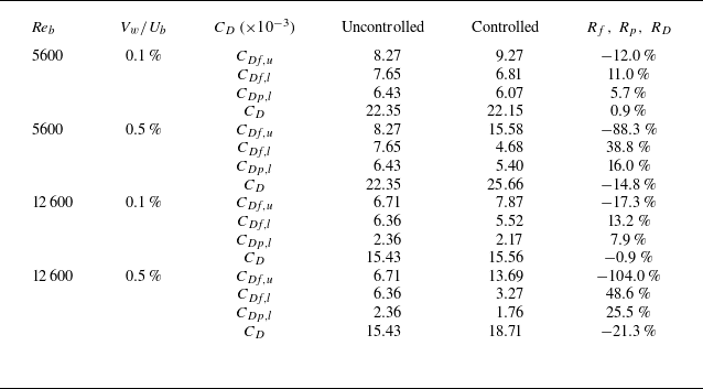
Similar to the opposition-controlled case, we investigate the dependence of the drag reduction effect on the bump height in the UB/US case. The componential and total drag coefficients in the uncontrolled and UB/US cases, and the corresponding reduction rates in the case with bump
 $h^+ \approx 40$
, are given in table 7, and shown graphically in figure 15. The trends observed in the case
 $h^+ \approx 40$
are similar to those in the case
 $h^+ \approx 20$
: an increase in the friction drag on the suction side, and a decrease in the friction drag and the pressure drag on the blowing side. The reduction rate of each drag coefficient is relatively similar to that in the case
 $h^+ \approx 20$
. In addition, similar to figures 12 and 14, we confirm also in the case
 $h^+ \approx 40$
(not shown here) that the flow separation is suppressed by the control, and the streamwise evolution of the drag coefficients is similar to that in the case
 $h^+ \approx 20$
. In other words, the dependence of the control effect by the UB/US on the bump height is small as compared with the opposition-controlled case.
Componential and total drag coefficients in the uncontrolled and UB/US cases, and the corresponding reduction rates in the case with bump height
 $h^+ \approx 40$
.

Decomposition of drag coefficient in the uncontrolled and UB/US cases: (a)
 ${\textit {Re}}_b = 5600$
,
 $h^+ \approx 20$
; (b)
 ${\textit {Re}}_b = 5600$
,
 $h^+ \approx 40$
; (c)
 ${\textit {Re}}_b = 12600$
,
 $h^+ \approx 20$
; (d)
 ${\textit {Re}}_b = 12600$
,
 $h^+ \approx 40$
.

According to the results in this subsection, UB significantly decreases not only the friction drag but also the pressure drag, leading to the suppression of the flow separation. In addition, the dependence of the bump height and Reynolds number on the control effect by the UB/US is relatively small compared with the opposition control.
3.3. Control effect on the flow separation
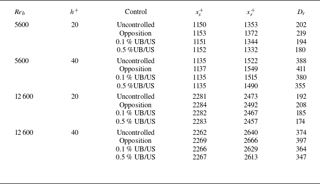
Finally, we investigate the control effect on the flow separation. Table 8 shows the flow separation point
 $x_s$
, reattachment point
 $x_r$
, and flow separation distance
 $D_r = x_r - x_s$
, in all cases. The flow separation position at each Reynolds number and bump height is hardly changed by the control. In the opposition-controlled (UB/US) case, the reattachment position shifts downstream (upstream), leading to an increase (decrease) in the flow separation distance. In addition, the flow separation distance decreases as the amplitude of UB/US increases. In other words, the opposition control and UB/US respectively enhance and suppress the flow separation. Furthermore, the flow separation is more suppressed by the large amplitude of UB/US, and these trends are independent of the Reynolds number and bump height.
Flow separation point
 $x_s$
, reattachment point
 $x_r$
, and flow separation distance
 $D_r = x_r - x_s$
, in all cases.

4. Conclusions
We have performed direct numerical simulations of a bump-installed turbulent channel flow controlled using two representative blowing/suction-based control methods, i.e. the opposition control (Choi et al. Reference Choi, Moin and Kim1994; Hammond et al. Reference Hammond, Bewley and Moin1998) and uniform blowing (UB) (Sumitani & Kasagi Reference Sumitani and Kasagi1995; Kametani & Fukagata Reference Kametani and Fukagata2011) accompanied by the same amount of uniform suction (US) on the other side of the wall. To investigate the control effect on the Reynolds number and the bump height, we consider two different Reynolds numbers
 ${\textit {Re}}_b = 5600$
and
 $12\,600$
, and bump heights
 $h^+ \approx 20$
and
 $40$
.
In the opposition-controlled case, we achieve the total drag reduction regardless of the Reynolds number and bump height. The friction drag reduction effect in the case with a bump is similar to that in the case without a bump, while the pressure drag reduction is hardly observed. The Reynolds number effect on the control effect is relatively small, similar to the case without the bump (Chang et al. Reference Chang, Collis and Ramakrishnan2002). The ratio of the pressure drag to the total drag increases as the bump height increases, resulting in a decrease in the total drag reduction rate against the increase of bump height.
In the UB/US case, the amount of the decrease in the friction drag on the blowing side wall (i.e. lower wall) is smaller than that of the increase in the friction drag on the suction side wall (i.e. upper wall), and the UB can reduce the pressure drag, unlike the opposition-controlled case. The enhancement of the turbulence in the blowing side suppresses the flow separation, leading to the pressure drag reduction. The dependence of the Reynolds number and bump height on the drag reduction effect is relatively small, as compared with the opposition-controlled case.
The present study reveals that the effect of a bump on the performance of turbulent drag reduction control is more complex than one might expect. Despite the attenuation of turbulence, which itself is similar to the streamwise travelling wave of spanwise wall oscillation studied by Banchetti et al. (Reference Banchetti, Luchini and Quadrio2020), the opposition control does not reduce the pressure drag. In contrast, the UB, which is usually considered to enhance flow separation, can suppress flow separation and pressure drag by a bump through turbulence enhancement. In both cases, the friction drag reduction is confirmed to be less sensitive to the presence of a bump. However, towards comprehensive understanding of whether the pressure drag and the total drag are reduced by different control methods under different conditions, a more systematic study should be designed and conducted in the future, focusing more on the local dynamics around the bump.
Acknowledgements
The authors are grateful to Dr S. Obi, Dr K. Ando, Dr L. Peng (Keio University) and Dr T. Kawata (Shibaura Institute of Technology) for fruitful discussions.
Funding
K.F. was supported by the Japan Society for the Promotion of Science (JSPS) through JSPS KAKENHI (grant nos 18H03758 and 21H05007).
Declaration of interests
The authors report no conflict of interest.
Data availability statement
The data that support the findings of this study are available from the corresponding author upon reasonable request.
Appendix A. Effect of bump height on the componential drag coefficients in the uncontrolled flow
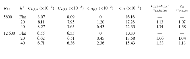
The componential drag coefficients in the uncontrolled cases at
 ${\textit {Re}}_b = 5600$
and
 $12\,600$
are summarised in table 9. As shown in table 9, the existence of a bump increases the total drag on the lower wall (
 $C_{Df,l}+C_{Dp,l}$
) and in the entire channel (
 $C_D$
) by
 $6$
–
 $74\,\%$
and
 $4$
–
 $38\,\%$
, respectively, compared with the case without a bump.
Componential drag coefficients in the uncontrolled case at
 $Re_b = 5600$
and
 $12\,600$
.

Appendix B. Drag reduction effect in the modified opposition-controlled case
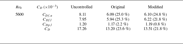
As a modified version of the opposition control, we apply the opposition control to only the region where the friction coefficient on the lower wall is positive; the control is turned off in the recirculation region where the friction coefficient on the lower wall is negative (the modified opposition control). Table 10 shows the componential drag coefficients in the original and modified opposition-controlled cases, and the corresponding reduction rates in the case at
 ${\textit {Re}}_b = 5600$
and
 $h^+ \approx 20$
. The friction coefficient on the upper wall and the pressure coefficient are hardly unchanged, whereas the friction drag coefficient on the lower wall in the modified opposition-controlled case is larger than that in the original opposition-controlled case. Therefore, the total reduction rate in the modified opposition-controlled case is smaller than that in the original opposition-controlled case.
Componential drag coefficients in the original and modified opposition-controlled cases, and the corresponding reduction rates in the case at
 ${\textit {Re}}_b = 5600$
and
 $h^+ \approx 20$
.

Appendix C. Control effect for RMS velocity fluctuations and RSS
The RMS of the velocity fluctuations and RSS in the case
 $h^+ \approx 20$
at (a)
 ${\textit {Re}}_b = 5600$
and (b)
 $Re_b=12\,600$
. Dashed for uncontrolled case, solid for opposition-controlled case. Note that in the plots of the RMS velocity fluctuations, red, green and blue lines represent
 $u_{{rms}}$
,
 $v_{{rms}}$
and
 $w_{{rms}}$
, respectively.

Figure 16 shows the RMS of velocity fluctuations and RSS in the case
 $h^+ \approx 20$
at
 ${\textit {Re}}_b = 5600$
and
 $12\,600$
in the opposition-controlled cases. As shown in this figure, the RMS velocity fluctuations are decreased in the upstream region and the region behind the bump. This means that the opposition control suppresses the turbulence intensities in these regions, similar to the case without a bump (Choi et al. Reference Choi, Moin and Kim1994). In addition, RMS velocity fluctuations are decreased also in the regions where the flow separation is observed
 $(x^+ \approx 1240)$
, leading to the extension of flow separation. However, in the region near the top of the bump (
 $x^+ \approx 1130$
),
 $u_{{rms}}$
is not suppressed so much by the control. It indicates that the opposition control cannot suppress the turbulence in the region near the top of the bump. Focusing on the RSS, it is significantly suppressed except for the downstream region of the bump (
 $x^+ \approx 1240$
). On the other hand, the RSS in the region near the wall at
 $x^+ \approx 1240$
(downstream) is hardly suppressed, indicating that the flow separation removes the control effect behind the bump.
The RMS of the velocity fluctuations and RSS in the case
 $h^+ \approx 20$
at (a)
 ${\textit {Re}}_b = 5600$
and (b)
 $Re_b=12\,600$
. Dotted for uncontrolled case, dashed for
 $0.1\,\%$
UB/US case, solid for
 $0.5\,\%$
UB/US case. Note that in the plots of the RMS velocity fluctuations, red, green and blue lines represent
 $u_{{rms}}$
,
 $v_{{rms}}$
and
 $w_{{rms}}$
, respectively.

Figure 17 shows the RMS of the velocity fluctuations and RSS in the case
 $h^+ \approx 20$
at
 ${\textit {Re}}_b = 5600$
and
 $12\,600$
in UB/US cases. Similar to the case without a bump (Sumitani & Kasagi Reference Sumitani and Kasagi1995), the RMS velocity fluctuations and RSS are increased (decreased) on the blowing (suction) side. In other words, the UB (US) enhances (suppresses) the turbulence intensity. The increased turbulence and enhanced mixing make the profile of mean streamwise velocity flattened. Since the RMS velocity fluctuations are also increased by the UB, suppression of the downward motions in the downstream region of the bump (green line in figure 13) can be explained in the same way.