2.1. Resolvent-based estimation

Consider the LNS equations and the flow state vector $\boldsymbol {q} = [\boldsymbol {u}\enspace \boldsymbol {v}\enspace \boldsymbol {w}\enspace \boldsymbol {p}]^\textrm {T}$, where $\boldsymbol {u}$, $\boldsymbol {v}$ and $\boldsymbol {w}$ are the streamwise, wall-normal and spanwise velocity components, $\boldsymbol {p}$ is the pressure component and $T$ denotes transpose. The flow state is decomposed according to the Reynolds decomposition $\boldsymbol {q} = \bar {\boldsymbol {q}} + \boldsymbol {q}^{\boldsymbol {\prime }}$, where $\bar {\boldsymbol {q}}$ is the mean flow (or, more generally, any base flow) and $\boldsymbol {q}^{\boldsymbol {\prime }}$ is the fluctuation around the base flow. The forcing $\boldsymbol {f}$ is obtained by gathering terms in the Navier–Stokes system that are nonlinear in the fluctuation $\boldsymbol {q}$. This decomposition is based on the LNS system considering only a molecular viscosity, and is exact if the forcing $\boldsymbol {f}$ is calculated considering all nonlinear terms. In the following, primes ($^{\prime }$) will be omitted for notational simplicity. For the channel flow configuration employed in this study, the linearised equations are written separately for each streamwise and spanwise wavenumber, such that the discretised state has a dimension equal to $4 N_y$, where $N_y$ is the number of wall-normal points. Taking advantage of the periodicity, Fourier transforms are applied in the streamwise and spanwise directions, i.e.

(2.1a)$$\begin{gather} \boldsymbol{q}(\alpha,y,\beta,t) = \int^{\infty}_{-\infty} \int^{\infty}_{-\infty} \boldsymbol{q}(x,y,z,t) \exp({-\textrm{i} \alpha x -\textrm{i} \beta z})\, {\textrm{d}\kern0.06em x}\,\textrm{d}z {,} \end{gather}$$

(2.1b)$$\begin{gather}\boldsymbol{f}(\alpha,y,\beta,t) = \int^{\infty}_{-\infty} \int^{\infty}_{-\infty} \boldsymbol{f}(x,y,z,t) \exp({-\textrm{i} \alpha x -\textrm{i} \beta z})\, {\textrm{d}\kern0.06em x}\,\textrm{d}z {,} \end{gather}$$

where $\alpha$ and $\beta$ denote the streamwise and spanwise wavenumbers, respectively, $x$, $y$ and $z$ indicate the streamwise, wall-normal and spanwise directions, respectively, and $t$ is time.

Writing the LNS equations in a discretised state-space form, considering a grid with $N_y$ points in the wall-normal direction, one has

(2.2a)$$\begin{gather} \boldsymbol{\mathsf{M}} \frac{\textrm{d} \boldsymbol{q}(t)}{\textrm{d} t} = \boldsymbol{\mathsf{A}} \boldsymbol{q}(t) + \boldsymbol{\mathsf{B}} \boldsymbol{f} {,} \end{gather}$$

(2.2b)$$\begin{gather}\boldsymbol{y}(t) = \boldsymbol{\mathsf{C}} \boldsymbol{q}(t) + \boldsymbol{n}(t) {,} \end{gather}$$

where $\boldsymbol{\mathsf{A}} \in \mathbb {C}^{4 N_{y} \times 4 N_{y}}$ is the linear operator, $\boldsymbol{\mathsf{B}} \in \mathbb {C}^{4 N_{y} \times 3 N_{y}}$ is the input matrix that restricts the forcing terms to appear only in the momentum equation, $\boldsymbol {y} \in \mathbb {C}^{N_{s}}$ is the system observation, $\boldsymbol{\mathsf{C}} \in \mathbb {C}^{N_{s} \times 4 N_{y}}$ is the observation matrix that selects $N_{s}$ sensor readings from the state vector and $\boldsymbol {n} \in \mathbb {C}^{N_{s}}$ is the measurement noise. Here $\boldsymbol{\mathsf{M}} \in \mathbb {C}^{4 N_{y} \times 4 N_{y}}$ is a diagonal matrix whose entries are set to one and zero for the momentum equations and continuity equations, respectively. Dependency on wavenumbers $\alpha$ and $\beta$, as well as on wall-normal variable $y$, were dropped to simplify notations. The flow forcing variables comprise $\boldsymbol {f} = [\boldsymbol {f}_{\boldsymbol {x}}\enspace \boldsymbol {f}_{\boldsymbol {y} }\enspace \boldsymbol {f}_{\boldsymbol {z}}]^\textrm {T} \in \mathbb {C}^{3 N_{y}}$, where $\boldsymbol {f}_{\boldsymbol {x}}$, $\boldsymbol {f}_{\boldsymbol {y}}$ and $\boldsymbol {f}_{\boldsymbol {z}}$ are the streamwise, wall-normal and spanwise forcing components, respectively (see Appendix A for details). If the forcing $\boldsymbol {f}$ in (2.2a) is defined as the nonlinear perturbation term in the Navier–Stokes system, the relation in (2.2a) is exact (McKeon & Sharma Reference McKeon and Sharma2010).

In the frequency domain, (2.2) is written as

(2.3)\begin{equation} \hat{\boldsymbol{y}}(\omega) = [\boldsymbol{\mathsf{C}} (- \textrm{i} \omega \boldsymbol{\mathsf{M}} - \boldsymbol{\mathsf{A}})^{{-}1} \boldsymbol{\mathsf{B}}]\, \hat{\boldsymbol{f}}(\omega) + \hat{\boldsymbol{n}}(\omega) {,} \end{equation}

where

(2.4)\begin{equation} \hat{\boldsymbol{y}} = \int\limits_{-\infty}^{\infty} \boldsymbol{y}(t) \textrm{e}^{\textrm{i} \omega t} \,\textrm{d}t \end{equation}

is the Fourier transform of $\boldsymbol {y}$, with analogous expression for other variables. Here $\omega$ is the temporal frequency and $\textrm {i} = \sqrt {-1}$. The term $\boldsymbol{\mathsf{R}} = (- \textrm {i} \omega \boldsymbol{\mathsf{M}} - \boldsymbol{\mathsf{A}})^{-1}$ is the resolvent operator, i.e. the transfer function between the forcing terms and the flow response (McKeon & Sharma Reference McKeon and Sharma2010; Cavalieri, Jordan & Lesshafft Reference Cavalieri, Jordan and Lesshafft2019; Towne et al. Reference Towne, Lozando-Durán and Yang2020). Appendix A contains the expressions for the linear operator $\boldsymbol{\mathsf{L}} = (- \textrm {i} \omega \boldsymbol{\mathsf{M}} - \boldsymbol{\mathsf{A}})$, input matrix $\boldsymbol{\mathsf{B}}$ and observation matrix $\boldsymbol{\mathsf{C}}$.

In the present study, we consider the observations of wall shear-stress components (${\textrm {d}u}/{\textrm {d} y}\vert _{wall}$ and ${\textrm {d}w}/{\textrm {d} y}\vert _{wall}$) and pressure ($p_{wall}$) on one or both walls for $Re_{\tau } \approx 180$ and $\approx 550$ cases (six sensors for each wavenumber), whereas for the $Re_{\tau } \approx 1000$ case, only wall shear stresses are available (four sensors for each wavenumber). As data is obtained directly from the DNS, measurement noise is non-existent. However, as will be shown later, measurement noise regularises the estimation, and thus the measurement noise $\hat {\boldsymbol {n}}$ was taken as a small value close to machine precision. This is analogous to the ill-posedness of Kalman-filter estimation for vanishing sensor noise. The small values are used in order to approach the zero-noise limit, justified by the high fidelity of the database, while keeping the estimation problem well posed.

Following Martini et al. (Reference Martini, Jordan, Cavalieri, Towne and Lesshafft2020), the optimal linear transfer function $\hat {\boldsymbol {T}}_{\boldsymbol {f}}$ between the system observation $\hat {\boldsymbol {y}}$ and the estimated flow forcing $\hat {\tilde {\boldsymbol {f}}}$,

(2.5)\begin{equation} \hat{\tilde{\boldsymbol{f}}} = \hat{\boldsymbol{T}}_{\boldsymbol{f}} \hat{\boldsymbol{y}} {,} \end{equation}

obtained by minimising the error between the true ($\hat {\boldsymbol {f}}$) and estimated ($\hat {\tilde {\boldsymbol {f}}}$) forcings, takes the form

(2.6)\begin{equation} \hat{\boldsymbol{T}}_{\boldsymbol{f}} = \boldsymbol{\mathsf{P}}_{\boldsymbol{\mathsf{ff}}} {\boldsymbol{\mathsf{R}}_{\boldsymbol{\mathsf{y}}}}^{*} \left(\boldsymbol{\mathsf{R}}_{\boldsymbol{\mathsf{y}}} \boldsymbol{\mathsf{P}}_{\boldsymbol{\mathsf{ff}}} {\boldsymbol{\mathsf{R}}_{\boldsymbol{\mathsf{y}}}}^{*} + \boldsymbol{\mathsf{P}}_{\boldsymbol{\mathsf{nn}}}\right)^{{-}1} {.} \end{equation}

In (2.6), $\boldsymbol{\mathsf{P}}_{\boldsymbol{\mathsf{ff}}} = \langle \hat {\boldsymbol {f}} \hat {\boldsymbol {f}}^* \rangle$ and $\boldsymbol{\mathsf{P}}_{\boldsymbol{\mathsf{nn}}} = \langle \hat {\boldsymbol {n}} \hat {\boldsymbol {n}}^* \rangle$ are the cross-spectral densities (CSDs) of the flow forcing and measurement noise statistics, respectively, and $\boldsymbol{\mathsf{R}}_{\boldsymbol{\mathsf{y}}} = \boldsymbol{\mathsf{C}} \boldsymbol{\mathsf{R}} \boldsymbol{\mathsf{B}}$ is the resolvent operator relating the forcing terms to the sensor readings. Here, $\langle \cdot \rangle$ denotes an ensemble average and the asterisk indicates a Hermitian transpose. If $\boldsymbol{\mathsf{P}}_{\boldsymbol{\mathsf{ff}}}$ is not known, which is frequently the case, it must be replaced by an a priori ansatz in order to evaluate the transfer function $\hat {\boldsymbol {T}}_{\boldsymbol {f}}$. Note that the forcing statistics are used to estimate instantaneous forces from sensors. An optimal linear estimator is obtained only if $\boldsymbol{\mathsf{P}}_{\boldsymbol{\mathsf{ff}}}$ is known (Martini et al. Reference Martini, Jordan, Cavalieri, Towne and Lesshafft2020). This, however, is typically not the case. For our estimates, we will consider three ansätze for the forcing CSD: the true CSD computed from DNS data, $\boldsymbol{\mathsf{P}}_{\boldsymbol{\mathsf{ff}},\boldsymbol{\mathsf{DNS}}}$; a spatially temporal white-noise assumption, $\boldsymbol{\mathsf{I}}$; and an eddy-viscosity model to (partially) account for the unknown forces (see Appendix A for the eddy-viscosity model linear operator formulation). Alternatively, Martini et al. (Reference Martini, Jordan, Cavalieri, Towne and Lesshafft2020) suggested a method to model the forcing statistics using additional sensors, but this is not pursued here.

Given the resolvent input–output formulation, the optimal state estimation is obtained from the optimal force estimation, i.e.

(2.7)\begin{equation} \hat{\tilde{\boldsymbol{q}}} = \boldsymbol{\mathsf{R}} \boldsymbol{\mathsf{B}} \hat{\tilde{\boldsymbol{f}}} {,} \end{equation}

where $\hat {\tilde {\boldsymbol {q}}}$ is the estimated flow state. The transfer function relating the system observation $\hat {\boldsymbol {y}}$ and the flow estimated state $\hat {\tilde {\boldsymbol {q}}}$ is thus obtained as

(2.8)\begin{equation} \hat{\boldsymbol{T}}_{\boldsymbol{q}} = \boldsymbol{\mathsf{R}} \boldsymbol{\mathsf{B}} \hat{\boldsymbol{T}}_{\boldsymbol{f}} {,} \end{equation}

hence,

(2.9)\begin{equation} \hat{\tilde{\boldsymbol{q}}} = \hat{\boldsymbol{T}}_{\boldsymbol{q}} \hat{\boldsymbol{y}} {.} \end{equation}

It is worth mentioning that the expression obtained for the transfer function $\hat {\boldsymbol {T}}_{\boldsymbol {f}}$ is closely related to Wiener filter estimation (Meditch Reference Meditch1973; Martinelli Reference Martinelli2009). More details and further discussion of the method employed to derive the estimator, including strategies for efficient computational implementation for large systems, can be found in Martini et al. (Reference Martini, Jordan, Cavalieri, Towne and Lesshafft2020).

Taking inverse Fourier transforms of (2.6) and (2.8), in order to return to the time domain, leads to

(2.10a)$$\begin{gather} \boldsymbol{T}_{\boldsymbol{f}}(\alpha,y,\beta,t) = \int^{\infty}_{-\infty} \hat{\boldsymbol{T}}_{\boldsymbol{f}}(\alpha,y,\beta,\omega) \textrm{e}^{\textrm{i} \omega t} \,\textrm{d}\omega {,} \end{gather}$$

(2.10b)$$\begin{gather}\boldsymbol{T}_{\boldsymbol{q}}(\alpha,y,\beta,t) = \int^{\infty}_{-\infty} \hat{\boldsymbol{T}}_{\boldsymbol{q}}(\alpha,y,\beta,\omega) \textrm{e}^{\textrm{i} \omega t} \,\textrm{d}\omega {.} \end{gather}$$

It is then possible to reconstruct the snapshots of the forcing and state estimates by performing a convolution of the transfer functions $\boldsymbol {T}_{\boldsymbol {f}}$ and $\boldsymbol {T}_{\boldsymbol {q}}$ with the measurements $\boldsymbol {y}$,

(2.11a)$$\begin{gather} \tilde{\boldsymbol{f}}(\alpha,y,\beta,t) = \int^{\infty}_{-\infty} \boldsymbol{T}_{\boldsymbol{f}}(\alpha,y,\beta,\tau) \boldsymbol{y}(\alpha,y,\beta,t-\tau) \,\textrm{d}\tau {,} \end{gather}$$

(2.11b)$$\begin{gather}\tilde{\boldsymbol{q}}(\alpha,y,\beta,t) = \int^{\infty}_{-\infty} \boldsymbol{T}_{\boldsymbol{q}}(\alpha,y,\beta,\tau) \boldsymbol{y}(\alpha,y,\beta,t-\tau) \,\textrm{d}\tau {,} \end{gather}$$

respectively.

Inverse Fourier transforms were also performed in the streamwise and spanwise directions to the estimates in space and time, i.e.

(2.12a)$$\begin{gather} \tilde{\boldsymbol{f}}(x,y,z,t) = \int^{\infty}_{-\infty} \int^{\infty}_{-\infty} \tilde{\boldsymbol{f}}(\alpha,y,\beta,t) \exp({\textrm{i} \alpha x + \textrm{i} \beta z} )\,\textrm{d}\alpha\,\textrm{d}\beta {,} \end{gather}$$

(2.12b)$$\begin{gather}\tilde{\boldsymbol{q}}(x,y,z,t) = \int^{\infty}_{-\infty} \int^{\infty}_{-\infty} \tilde{\boldsymbol{q}}(\alpha,y,\beta,t) \exp({\textrm{i} \alpha x + \textrm{i} \beta z})\,\textrm{d}\alpha\,\textrm{d}\beta {.} \end{gather}$$

The formulation above may also be entirely written in space and time, with forcing and state estimated by a space–time convolution between $\hat {\boldsymbol {y}}$ and the transfer functions. However, the use of periodic boundary conditions in the channel-flow simulations allows the evaluation of each wavenumber separately, which is more computationally efficient.

As a final remark, note that the convolutions in (2.11) lead to non-causal estimations. This is intrinsic to the frequency-domain approach, and prevents its direct application in real time, as is necessary for flow control. The goal of this work to thoroughly investigate which flow structures may be accurately estimated with a linear model from wall sensors. Thus, without restrictions related to causality, we here evaluate which turbulent structures leave a wall imprint allowing them to be estimated from a time series of wall measurements. A causal extension is nonetheless possible via the Wiener–Hopf formalism, as discussed in Martinelli (Reference Martinelli2009) and Martini (Reference Martini2019).

2.2. Numerical simulations

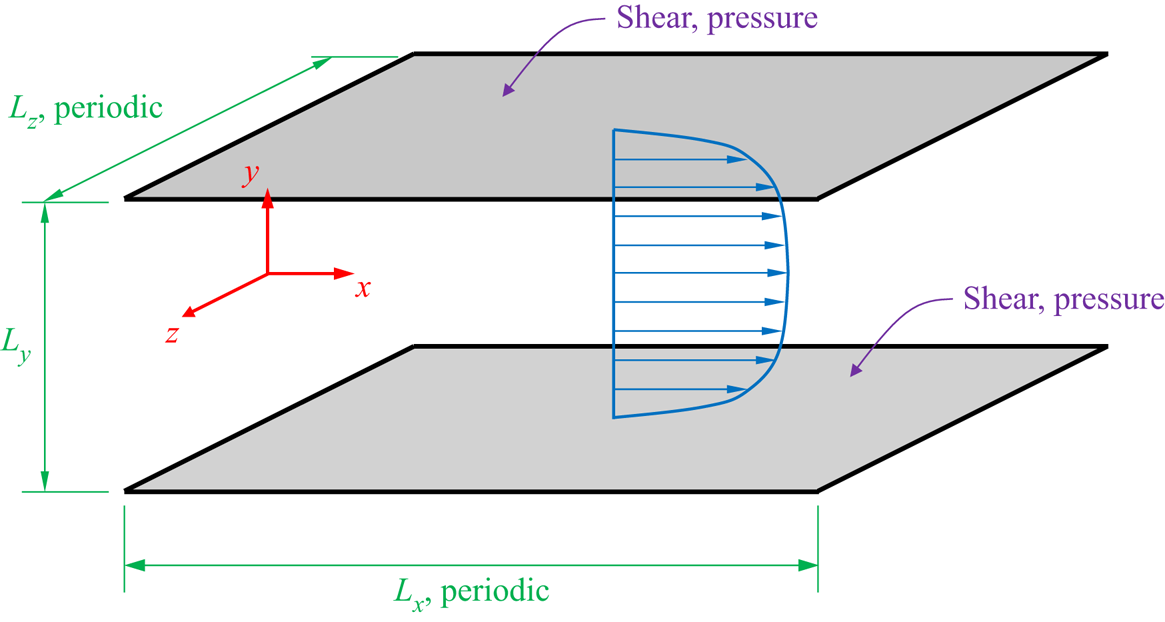
The DNS were conducted with the Channelflow pseudospectral code (Gibson et al. Reference Gibson2019). Figure 1 shows a sketch of the geometry and coordinate system of the problem. The box dimensions were $2{\rm \pi} \times 2 \times {\rm \pi}$ in the streamwise ($L_x$), wall-normal ($L_y$) and spanwise ($L_z$) directions, respectively, for the $Re_{\tau } \approx 550$ and 1000 cases, whereas a box of $4{\rm \pi} \times 2 \times 2{\rm \pi}$ dimensions was employed for the $Re_{\tau } \approx 180$ simulation. Periodic boundary conditions are assumed in the streamwise and spanwise directions. The wall-normal direction ($y$) was discretised with Chebyshev polynomials, using the same number of polynomials as other simulations (Lozano-Durán & Jiménez Reference Lozano-Durán and Jiménez2014), and the streamwise ($x$) and spanwise ($z$) directions were discretised using Fourier modes, including dealiasing (Del Álamo et al. Reference Del Álamo, Jiménez, Zandonade and Moser2004).

Figure 1.

Sketch of the channel flow geometry, coordinate system (red), mean flow (blue) and wall measurements employed to perform the estimations (grey).

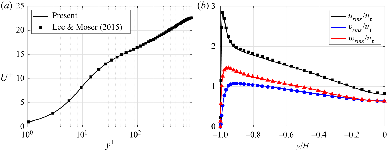
The DNS databases for $Re_{\tau } \approx 180$ and 550 were validated by Martini et al. (Reference Martini, Jordan, Cavalieri, Towne and Lesshafft2020) and Morra et al. (Reference Morra, Nogueira, Cavalieri and Henningson2021), respectively, using earlier simulations by Del Álamo & Jiménez (Reference Del Álamo and Jiménez2003). We validate the $Re_{\tau } \approx 1000$ database against results from Lee & Moser (Reference Lee and Moser2015) in figure 2. In the figure, $H$ denotes the channel half-height, $y^+$ is the wall-normal position in inner (viscous) units, $U^+$ is the mean velocity profile in inner units, $u$, $v$ and $w$ correspond to the streamwise, wall-normal and spanwise velocity components, subscript $rms$ indicates root mean square (r.m.s.) values and $u_{\tau }$ is the friction velocity. Good agreement is observed, validating the present database.

Figure 2.

The $Re_{\tau } \approx 1000$ channel flow DNS validation results. Lines indicate the present simulations results and symbols denote data from Lee & Moser (Reference Lee and Moser2015). (a) Mean velocity profile ($U^{+}$) and (b) r.m.s. values for each velocity component.

Table 1 shows, among other information, the Reynolds numbers (based on the friction velocity $u_{\tau }$, i.e. $Re_{\tau }$, and channel half-height $H$ and bulk velocity $U_b$, i.e. $Re$), number of mesh points ($N_x$, $N_y$ and $N_z$) and mesh discretisation ($\Delta x^{+}$, $\Delta z^{+}$, $\Delta {y_{min}}^{+}$ and $\Delta {y_{max}}^{+}$). In all cases, a plus superscript indicates non-dimensional quantities using inner (viscous) scaling. Quantities expressed in outer units are denoted without the plus superscript and are normalised by the bulk velocity and channel half-height. The number of wavenumbers in the streamwise and spanwise directions in the DNS is $3/2$ times higher than the $N_x$ and $N_z$ values reported in table 1 for dealiasing. The number of snapshots ($N_t$) and the time steps based on inner units ($\Delta t^{+}$) are also exhibited in the table. In the simulations, initial transients, detected by evaluating the turbulent kinetic energy and the friction coefficient on the walls were discarded, thus the snapshots retained are within the statistical steady state. The number of time steps ($N_{fft}$) in each block of data and the number of blocks ($N_b$) used within Welch's method (Welch Reference Welch1967) to estimate the CSDs and power spectral densities (PSDs) of DNS and estimation data are also provided in table 1. A Hann window and 75 % overlap were used to compute spectra.

Table 1.

Channel flow DNS parameters for the cases studied.

In order to reduce computational cost and storage requirements, the DNS data (state and forcing terms) were then filtered, retaining a lower number of wavenumbers in the streamwise and spanwise directions, e.g. $N_{\alpha } = 31$ and $N_{\beta } = 32$ for the $Re_{\tau } \approx 550$ case (see table 2 and Appendix B). Following this strategy, it was possible to compress the data, reducing the storage and memory needed to perform, a posteriori, the resolvent-based estimations. As an example, for $Re_{\tau } \approx 550$, a total of $N_x$ and $N_z$ discrete $\alpha$ and $\beta$, respectively, are possible for the current mesh parameters, i.e. the database was compressed by a factor of approximately 148. Note that we make use of the property $\boldsymbol {q}(\alpha ,y,\beta ,t) = \boldsymbol {q}^{*}(-\alpha ,y,-\beta ,t)$. The cutoff values for $\alpha$ and $\beta$ were defined based on the premultiplied power-spectral peak at a wall-normal distance of $y^{+} = 15$, i.e. $({\lambda _x}^{+}$, ${\lambda _z}^{+}) \approx (1000,100)$ (Del Álamo & Jiménez Reference Del Álamo and Jiménez2003), where ${\lambda _x}^{+}$ and ${\lambda _z}^{+}$ are the streamwise and spanwise wavelengths in wall units. The $\alpha$ and $\beta$ cutoff values were chosen such that all the cases include the wavenumber corresponding to $({\lambda _x}^{+},{\lambda _z}^{+}) \approx (1000,100)$, ensuring that the premultiplied power-spectral peak is contained within the data. The smaller flow structures are filtered as a consequence of data compression, but this does not impact the estimation of the retained wavenumbers due to the linearity of the estimator. Table 2 provides the precise cutoff values in outer ($\alpha _{cut}$ and $\beta _{cut}$) an inner (${\alpha _{cut}}^{+}$ and ${\beta _{cut}}^{+}$) units.

Table 2.

Wavenumber cutoff values used to filter the DNS databases.

3.1. Estimation of a sample snapshot

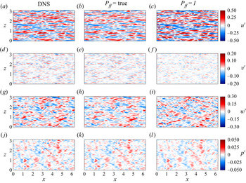
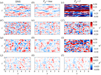
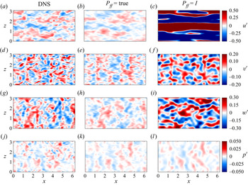
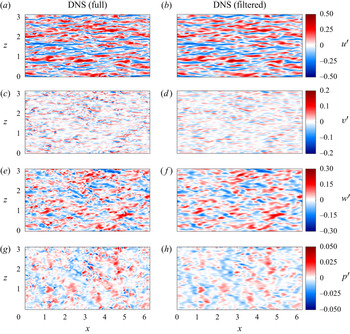
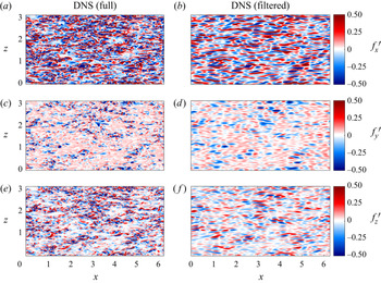
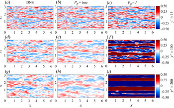
To provide a first observation of the estimated structures in the turbulent field, we begin by comparing flow estimate and DNS results for sample snapshots, taken at some reference wall-parallel planes. Filtered DNS snapshots, retaining only the wavenumbers considered in the estimations, are displayed in the figures to enable direct comparisons; Appendix B shows DNS snapshots without the application of the spatial filtering for the state and forcing components. Snapshots of flow field state and forcing estimates are shown in figures 3–6. Figures 3 and 4 show, respectively, state and forcing estimates in the buffer layer, at $y^{+} \approx 15$, and figures 5 and 6 show state estimates at $y^{+} \approx 100$ and 200. In all cases, estimates from wall measurements are compared with the DNS results. When the true forcing statistics are considered ($\boldsymbol{\mathsf{P}}_{\boldsymbol{\mathsf{ff}}} = \boldsymbol{\mathsf{P}}_{\boldsymbol{\mathsf{ff}},\boldsymbol{\mathsf{DNS}}}$), the resemblance is remarkable between the filtered DNS and the resolvent-based estimates of all flow state components in the buffer layer, at a wall-normal distance of $y^{+} \approx 15$ (figure 3). Even when the forcing CSD is approximated as white noise ($\boldsymbol{\mathsf{P}}_{\boldsymbol{\mathsf{ff}}} = \boldsymbol{\mathsf{I}}$), close agreement between the DNS and estimated states is observed for $y^{+} \approx 15$. Both estimates were able to recover the near-wall streaks of streamwise velocity $u$, as well as the structures for other velocity components and pressure.

Figure 3.

Comparison between filtered DNS and resolvent-based estimates of an instantaneous snapshot of the flow state for $Re_{\tau } \approx 550$, $y^{+} \approx 15$ and using wall measurements of pressure and shear stress. Panels (a,d,g, j), (b,e,h,k) and (c, f,i,l) are DNS data, true and white-noise forcing estimates, respectively. Panels (a,b,c), (d,e, f), (g,h,i) and ( j,k,l) are streamwise ($u^{\prime }$), wall-normal ($v^{\prime }$), spanwise ($w^{\prime }$) velocity fluctuations and pressure fluctuation ($p^{\prime }$), respectively. Fluctuations shown in outer units. An animated version of this figure showing its time evolution is provided in the supplementary movies.

Figure 4.

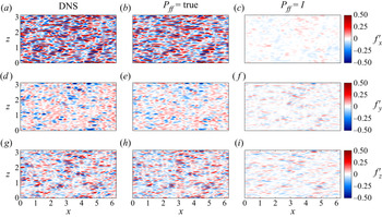
Comparison between filtered DNS and resolvent-based estimates of an instantaneous snapshot of the flow forcing components for $Re_{\tau } \approx 550$, $y^{+} \approx 15$ and using wall measurements of pressure and shear stress. Panels (a,d,g), (b,e,h) and (c, f,i) are DNS data, true forcing and white-noise forcing estimates, respectively. Panels (a,b,c), (d,e, f) and (g,h,i) are streamwise ($\,f_{x}^{\prime }$), wall-normal ($\,f_{y}^{\prime }$) and spanwise ($\,f_{z}^{\prime }$) forcing fluctuation components, respectively. Fluctuations shown in outer units.

Figure 5.

Comparison between filtered DNS and resolvent-based estimates of an instantaneous snapshot of the flow state for $Re_{\tau } \approx 550$, $y^{+} \approx 100$ and wall measurements of pressure and shear stress. See comments in the caption of figure 3.

Figure 6.

Comparison between filtered DNS and resolvent-based estimates of an instantaneous snapshot of the flow state for $Re_{\tau } \approx 550$, $y^{+} \approx 200$ and wall measurements of pressure and shear stress. See comments in the caption of figure 3.

Figure 4 shows snapshots of the forcing components. Good agreement between filtered DNS data and estimates is achieved, i.e. most of the structures present on the DNS were captured by the estimates. Note that although the true colour was employed as the forcing CSD ansatz in (2.6) to obtain the results displayed in the figure, the estimated forcing components were not exactly recovered, as the system observation was restricted to the wall measurements of shear stresses and pressure. Forcing estimates obtained with the white-noise forcing ansatz have a significant mismatch with the DNS reference values.

Figures 5 and 6 show the state-estimate snapshots in the logarithmic layer, at $y^{+} \approx 100$ and $\approx 200$, respectively, for $Re_{\tau } \approx 550$. These are more challenging estimates, as they involve positions farther from the wall, where measurements are taken. The estimates were not as accurate as the previous results obtained for $y^{+} \approx 15$ (figure 3). Nevertheless, most of the large-scale structures present in the DNS snapshots were well captured by the estimation procedure, even for $y^{+} \approx 200$. Far from the wall, the white-noise forcing assumption does not lead to results of the same quality as the those obtained close to the wall (figure 3). Such results are in line with recent works (Illingworth et al. Reference Illingworth, Monty and Marusic2018; Abreu et al. Reference Abreu, Cavalieri, Schlatter, Vinuesa and Henningson2020a; Morra et al. Reference Morra, Nogueira, Cavalieri and Henningson2021), which have shown that considering the forcing CSD to be white noise in a resolvent formulation leads to reasonable models for near-wall structures but significant mismatch for larger-scale structures at higher wall-normal positions.

Most structures within the velocity field are faithfully recovered by the estimates using the true forcing statistics, albeit with somewhat lower amplitude than the DNS fields in many cases. On the other hand, when white-noise forcing is considered, shown in figure 3(c, f,i,l), amplitudes were overestimated. Only the pressure component could be estimated with reasonable accuracy using the white-noise forcing assumption. This is likely related to the non-local behaviour of pressure fluctuations, which are related to the global velocity fluctuations by a Poisson equation (Anantharamu & Mahesh Reference Anantharamu and Mahesh2020); thus, pressure fluctuations tend to be more spatially extended, simplifying their estimation from wall measurements. Forcing-component estimates are not displayed, as the estimates were less accurate than those shown in figure 4, especially regarding their amplitudes.

3.2. Effect of the choice of sensors

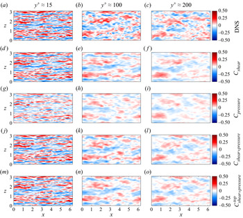
Figure 7 displays snapshots of the streamwise velocity component from the DNS and estimates obtained with different definitions for the observation matrix $\boldsymbol{\mathsf{C}}$, i.e. sensors accounting for the wall shear stress only (${\textrm {d}u}/{\textrm {d} y}\vert _{wall}$ and ${\textrm {d}w}/{\textrm {d} y}\vert _{wall}$), wall pressure only ($p_{wall}$) and both wall shear stress and pressure. The measurements were taken at both top and bottom channel walls (figure 7d–l) and only on the channel top wall (figure 7m–o), for the $Re_{\tau } \approx 550$ case and three wall-normal positions, i.e. $y^{+} \approx 15$, 100 and 200, which are shown in figure 7(a,d,g, j,m), figure 7(b,e,h,k,n) and figure 7(c, f,i,l,o), respectively. To compare the different estimates, true forcing statistics were used.

Figure 7.

Comparison between DNS and true forcing statistics of the streamwise velocity estimates obtained with different definitions for the observation matrix $\boldsymbol{\mathsf{C}}$ for $Re_{\tau } \approx 550$. Panels (a,d,g, j,m), (b,e,h,k,n) and (c, f,i,l,o) are $y^{+} \approx 15$, 100 and 200, respectively. Panels (a,b,c), (d,e, f), (g,h,i), ( j,k,l) and (m,n,o) are DNS, observation $\boldsymbol{\mathsf{C}}$ containing only the wall shear stress (${\textrm {d}u}/{\textrm {d} y}\vert _{wall}$ and ${\textrm {d}w}/{\textrm {d} y}\vert _{wall}$) on both walls, observation $\boldsymbol{\mathsf{C}}$ containing only the wall pressure ($p_{wall}$) on both walls, observation $\boldsymbol{\mathsf{C}}$ containing both wall shear stress and pressure (${\textrm {d}u}/{\textrm {d} y}\vert _{wall}$, ${\textrm {d}w}/{\textrm {d} y}\vert _{wall}$ and $p_{wall}$) on both walls and observation $\boldsymbol{\mathsf{C}}$ containing both wall shear stress and pressure (${\textrm {d}u}/{\textrm {d} y}\vert _{wall}$, ${\textrm {d}w}/{\textrm {d} y}\vert _{wall}$ and $p_{wall}$) only on the top wall, respectively. Fluctuations shown in outer units. An animated version of this figure is provided in the supplementary movies available at https://doi.org/10.1017/jfm.2021.764.

The estimates are less accurate when only observations of the pressure on both walls are considered. When both wall shear stress and pressure are provided to evaluate the transfer function between the measurements and estimated state, better results are achieved. The case where only the wall shear stress is used displays an intermediate performance, only slightly worse than estimates from wall shear stress plus wall pressure. Using both shear stress and pressure at just one wall (the one closer to the wall-normal planes where the results are evaluated) leads to estimates of a similar quality to those obtained with measurements at both walls. Appendix C shows comparison metrics for the different observation definitions to corroborate these conclusions.

3.3. Estimation with the linearised operator including eddy-viscosity

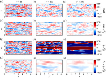
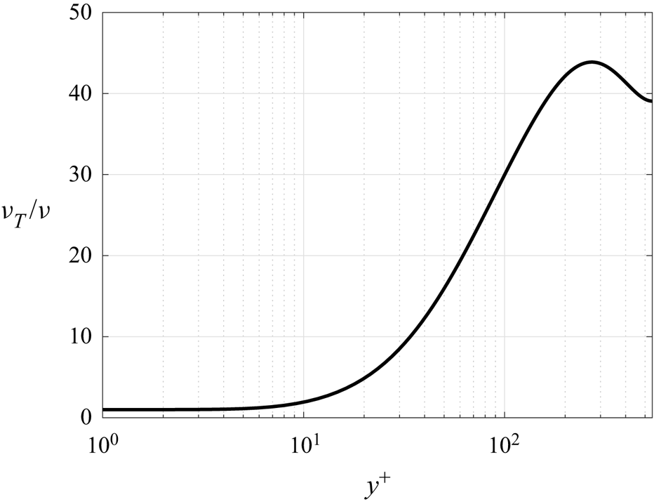
Earlier works have obtained flow estimates using a linearised operator including eddy viscosity (Illingworth et al. Reference Illingworth, Monty and Marusic2018; Towne et al. Reference Towne, Lozando-Durán and Yang2020) and white-noise forcing. Such a model attempts to partially represent the colour of the nonlinear terms of the Navier–Stokes system, which improves predictions obtained from the resolvent framework (Morra et al. Reference Morra, Semeraro, Henningson and Cossu2019). To make comparisons with this approach, we employ the same methodology used by Towne et al. (Reference Towne, Lozando-Durán and Yang2020), which considers the total viscosity $\nu _T$; Appendix A shows the linear operator formulation. This approach will be referred to as the eddy-viscosity model. Figure 8 exhibits the estimates for the $Re_{\tau } \approx 550$ case and three wall-normal positions, similar to figure 7, but with the rows representing the DNS results and true, white and eddy-viscosity model ($\nu _T$) estimates. Only streamwise velocity component results are displayed in the figure, and similar snapshot reconstructions were obtained for the other state components.

Figure 8.

Comparison between DNS and estimates considering the eddy-viscosity model. Streamwise velocity component ($u^{\prime }$) snapshots for $Re_{\tau } \approx 550$. Panels (a,d,g, j), (b,e,h,k) and (c, f,i,l) are $y^{+} \approx 15$, 100 and 200, respectively. Panels (a,b,c), (d,e, f) and (g,h,i) are DNS data and estimates using the true, white noise and eddy-viscosity forcing models, respectively. Fluctuations shown in outer units. An animated version of this figure is provided in the supplementary movies.

The use of the eddy-viscosity model prevented the large amplitude overprediction in the estimates observed in the white-noise forcing case and is thus an option when the forcing statistics are unknown. At the same time, the estimates obtained using the eddy-viscosity model are significantly worse than those obtained using the true forcing statistics from the DNS. Another aspect worthy of mention is the eddy-viscosity model has a dual effect on the estimations compared with the white-noise forcing statistics: while it improves estimates of large-scale coherent structures farther from the wall ($y^{+} \approx 100$ and 200 snapshots), it worsens the estimates of near-wall structures ($y^{+} \approx 15$). Improved results could be obtained if, instead of using the standard Cess model (see Appendix A), the eddy-viscosity model were to be calibrated for each friction Reynolds number (Pickering et al. Reference Pickering, Rigas, Schmidt, Sipp and Colonius2021). However, our goal is not to find the optimal viscosity model for the flow, but rather to show that these models can improve the estimation by acting as a surrogate for the true, but unknown, force colour.

Several studies with linearised models showed better agreement with turbulence statistics when an eddy viscosity is included in the linearised operator (Del Álamo & Jiménez Reference Del Álamo and Jiménez2006; Hwang & Cossu Reference Hwang and Cossu2010; Morra et al. Reference Morra, Semeraro, Henningson and Cossu2019; Pickering et al. Reference Pickering, Rigas, Schmidt, Sipp and Colonius2021). As discussed by Morra et al. (Reference Morra, Nogueira, Cavalieri and Henningson2021), the inclusion of an eddy viscosity may be seen as the introduction of some forcing colour to the linearised operator based on the molecular viscosity. Although this is not exact, this modelling approach is found to improve predictions from the linearised system, particularly for large-scale structures, as seen in the present estimates using white-noise forcing (figure 8g–i and figure 8j–l). However, despite these improvements, the consideration of white-noise forcing in an operator that includes an eddy viscosity is still an approximation that leads to errors for a number of structures, as recently discussed by Symon et al. (Reference Symon, Illingworth and Marusic2021). Use of the actual statistics of nonlinear terms from a simulation leads to an exact agreement in the input–output system by construction (Towne et al. Reference Towne, Schmidt and Colonius2018; Morra et al. Reference Morra, Nogueira, Cavalieri and Henningson2021), and this is, therefore, the best-case scenario for a linearised estimator. This is confirmed by the superior performance of estimates using $\boldsymbol{\mathsf{P}}_{\boldsymbol{\mathsf{ff}}} = \boldsymbol{\mathsf{P}}_{\boldsymbol{\mathsf{ff}},\boldsymbol{\mathsf{DNS}}}$ compared with the other modelling strategies. However, this comes with the additional requirement of forcing statistics, leading to a more complex procedure, as discussed in § 3.5.

3.4. Statistics of the estimated flow

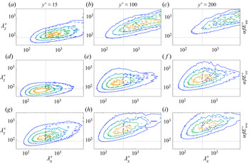
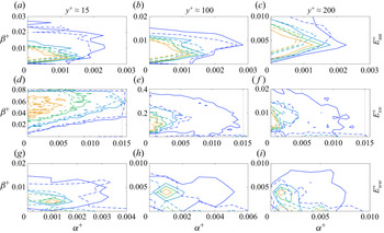
Figures 9 and 10 show the power spectra of velocity components with and without premultiplication, respectively, for different wall-normal distances. Premultiplication of spectra by $\alpha$ and $\beta$ highlights smaller-scale fluctuations, which are not accurately estimated from wall measurements, as seen in figures 5 and 6; hence, we have also included spectra without premultiplication in figure 10 for a clearer visualisation of the energy content of the largest scales in the simulation. The estimates were evaluated using the true forcing statistics. Continuous and dashed lines represent the power spectra computed from the full DNS snapshots (without filtering) and the resolvent-based estimates, respectively. Four equally spaced contour levels are plotted and all levels are normalised by the peak value of the DNS spectra for each state component and wall-normal distance. The dotted lines indicate the wavenumber cutoff; only spectral values in the first quadrant, formed by the intersection of these crossing lines, i.e. the top right-hand portion of each panel, are estimated.

Figure 9.

Premultiplied power spectra comparison between DNS (solid lines) and resolvent-based estimates considering true forcing statistics (dashed lines) and wall measurements of pressure and shear stress for $Re_{\tau } \approx 550$. Panels (a,d,g, j), (b,e,h,k) and (c, f,i,l) are $y^{+} \approx 15$, 100 and 200, respectively. Panels (a,b,c), (d,e, f) and (g,h,i) are streamwise ($\alpha \beta {E_{uu}}^+$), wall-normal ($\alpha \beta {E_{vv}}^+$) and spanwise ($\alpha \beta {E_{ww}}^+$) velocity and pressure ($\alpha \beta {E_{pp}}^+$) premultiplied power spectra, respectively. Contour levels equally spaced between 0.2 and 0.8 times the peak value of the DNS. Dotted lines indicate the wavenumbers cutoff quadrant.

Figure 10.

Power spectra comparison between DNS (solid lines) and resolvent-based estimates using true forcing statistics (dashed lines) and wall measurements of pressure and shear stress for $Re_{\tau } \approx 550$. Panels (a,d,g, j), (b,e,h,k) and (c, f,i,l) are $y^{+} \approx 15$, 100 and 200, respectively. Panels (a,b,c), (d,e, f), (g,h, i) and (j,k,l) are streamwise (${E_{uu}}^+$), wall-normal (${E_{vv}}^+$) and spanwise (${E_{ww}}^+$) velocity and pressure (${E_{pp}}^+$) power spectra, respectively. See comments in the caption of figure 9.

The agreement between the DNS and estimates is excellent for all state components at a wall-normal distance of $y^{+} \approx 15$, consistent with the observations of figure 3. The peak in the premultiplied power spectrum at $({\lambda _x}^{+},{\lambda _z}^{+}) \approx (1000,100)$ is accurately estimated for the streamwise velocity component at $y^{+} \approx 15$. At this wall-normal distance, the peak energies of the other state components are also captured by the estimates. However, for the pressure component, only a portion of the peak was estimated, as the bulk containing the most energetic part of the spectrum lies outside the observable wavenumber parameters. Farther from the wall, the estimated spectra progressively deteriorate. This effect appears stronger in the premultiplied spectra of figure 9, which highlights smaller structures, while spectra without premultiplication, which highlights larger scales, show a better agreement, with the estimation leading to some underestimation of the peak power.

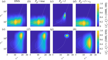
Figure 11 shows the PSD of the streamwise velocity as a function of the wall-normal coordinate ($y^{+}$) and phase speed $c^{+} = \omega ^{+}/\alpha ^{+}$ for two combinations of $({\lambda _x}^{+},{\lambda _z}^{+})$, i.e. $\approx (1000,100)$ and $(3400,850)$. Such wavenumber combinations correspond to the near-wall and large-scale structures, respectively, extracted from peaks of premultiplied spectra for the $Re_{\tau } \approx 550$ case (Morra et al. Reference Morra, Nogueira, Cavalieri and Henningson2021). In the figure, the dashed lines represent the mean velocity profile in plus units. The position of peak PSD $(y^{+}, c^{+})$ is related to the critical layer ($U^{+} = c^{+}$), as expected from an analysis of the resolvent operator (McKeon & Sharma Reference McKeon and Sharma2010; Tissot et al. Reference Tissot, Zhang, Lajús, Cavalieri and Jordan2017). The white-noise forcing assumption is only able to estimate the PSD peak, which follows the critical layer, whereas the estimates obtained using the true forcing statistics are closer to the DNS results. This shows that incorporating the forcing colour produces a model that is able to capture the bulk of the energy that lies outside the critical-layer position. When the eddy-viscosity model is considered, the white-noise forcing results are improved, especially for the wavenumber pair related to the near-wall structures, but errors are nonetheless present for larger structures.

Figure 11.

Comparison between DNS and resolvent-based estimates of the streamwise velocity PSDs for $Re_{\tau } \approx 550$ using wall measurements of pressure and shear stress. The PSD contour plots are normalised by the peak value at each frame. The dashed lines indicate the mean velocity profile in plus units ($U^{+}$). Panels (a,e), (b, f), (c,g) and (d,h) are DNS data, true, white noise and eddy-viscosity model estimates, respectively. Here (a–d) $({\lambda _x}^{+},{\lambda _z}^{+}) \approx (1000,100)$ (near-wall structures) and (e–h) $({\lambda _x}^{+},{\lambda _z}^{+}) \approx (3400,850)$ (large-scale structures).

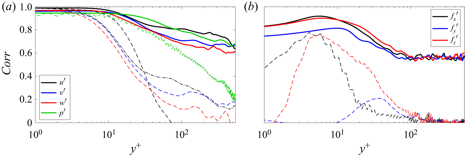
Normalised correlations between the filtered DNS data and resolvent-based estimates are shown in figure 12. The correlation metric is defined as

(3.1)\begin{equation} Corr(x,y,z) = \frac{\displaystyle\int {q_{DNS}}\left(x,y,z,t\right) {q_{est}}\left(x,y,z,t\right) \textrm{d}t}{\sqrt{\displaystyle\int {{q_{DNS}}\left(x,y,z,t\right)}^2 \,\textrm{d}t} \sqrt{\displaystyle\int {{q_{est}}\left(x,y,z,t\right)}^2 \,\textrm{d}t}} {,} \end{equation}

where $t$ is the time, $q$ denotes the perturbation component (e.g. pressure or a particular velocity or forcing component) and $y$ is the wall-normal coordinate. Subscripts $est$ and $DNS$ denote estimate and simulation quantities, respectively. To evaluate the correlation values, we employed probes traversing the channel wall-normal direction at $(x, z) = (0, 0)$ scanning the complete time series. For all metrics computed in this work, the first and last $N_{fft}/2$ instants of the time series were discarded as they could not be estimated due to end effects when computing the convolution (2.11) using finite data.

Figure 12.

Correlation between filtered DNS and estimate data for $Re_{\tau } \approx 550$ case and wall measurements of shear stress and pressure. Panels (a) and (b) show the flow state and forcing components, respectively. Continuous, dashed and dash–dotted lines denote estimates obtained with true forcing statistics, white-noise and the eddy-viscosity model, respectively.

Both state- and forcing-component correlations are shown in figure 12 and the estimates were evaluated using true (continuous lines) and white-noise (dashed lines) forcing. For the eddy-viscosity model (dash–dotted lines), only the streamwise velocity component is plotted, as similar behaviour is observed for the other state and forcing components. Up to $y^{+} \approx 15$, the normalised correlation is higher than 0.95 and 0.65 for all state and forcing components, respectively, when using true forcing statistics. For higher wall-normal distances the correlation decays, but values higher than 0.6 for the state components are obtained up to $y^{+} \approx 550$. It is clear from the normalised correlation values that modelling the forcing as white noise is only accurate for distances very close to the wall, where the measurements are obtained. For $y^{+} \geq 10$, the correlation drastically decays, reaching values below zero (the normalised correlations is defined between $-1$ and 1) for the streamwise velocity component at $y^{+} \approx 70$. When the eddy-viscosity model is considered, lower correlation values than those observed for the white-noise forcing estimates are observed near the wall, however, for distances higher than $y^{+} \approx 30$, the linear operator containing the eddy-viscosity displayed an intermediate correlation, between white and true forcing statistics estimates. Forcing correlation values are not as good as those observed for the state components, reaching a maximum of approximately 0.85 at $y^{+} \approx 6$, for the streamwise forcing component, and stabilising at approximately 0.45 for $y^{+} \geq 100$ when considering true forcing statistics.

Note that the white-noise assumption produced a sawtooth-like curve for the estimated pressure. Such a feature is also observed for the estimated pressure CSD (in frequency domain) and for the subsequent statistics presented in this paper and we conjecture that it is related to the white-noise forcing assumption. Estimates with a quasi-white forcing CSD, with coherence length equal to twice the maximal grid spacing, eliminates such oscillations, but such an assumption is not employed in this study.

Figure 13 shows normalised r.m.s. errors for state- and forcing-component estimates with respect to the filtered DNS. The r.m.s. error is given by

(3.2)\begin{equation} Err(x,y,z) = \frac{\displaystyle\sqrt{\int \left({q_{est}}\left(x,y,z,t\right) - {q_{DNS}}\left(x,y,z,t\right)\right)^2\,\textrm{d}t}}{\displaystyle{\sqrt{\int {q_{DNS}}\left(x,y,z,t\right)^2 \,\textrm{d}t}}} {.} \end{equation}

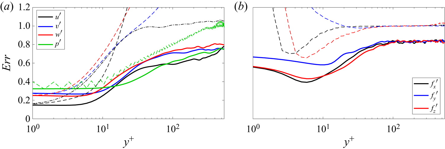
Lower errors are obtained from estimates using true forcing statistics (continuous lines) than white-noise forcing (dashed lines). Once again, only the streamwise velocity component is shown for the eddy-viscosity model (dashed lines), which reduced the error compared with the white-noise forcing estimate. These results are in accordance with the previous correlation values (figure 12) and estimated snapshots (figures 3–6 and 8). For the state estimates obtained using true forcing statistics, near the wall the normalised error is approximately constant up to $y^{+} \approx 5$ and then increases towards the channel centre. Interestingly, the normalised error at $y^{+} \approx 550$ is approximately 0.77 for all state components. For the three forcing components, the normalised error initially decays, up to $y^{+} \approx 10$, then reaches a maximum value of approximately 0.82 at $y^{+} \approx 80$ which remains almost constant up to $y^{+} \approx 550$. White-noise forcing and the eddy-viscosity model assumptions produce high errors that far exceed the axis limits selected to highlight the results obtained using true forcing statistics and the eddy-viscosity model (peak error values for white-noise forcing were 46.12, 1.60, 2.82, 790.64, 20789 and 1590 for $u^{\prime }$, $v^{\prime }$, $w^{\prime }$, ${f_x}^{\prime }$, ${f_y}^{\prime }$ and ${f_z}^{\prime }$, respectively).

Figure 13.

Normalised r.m.s. error between filtered DNS and estimate data for $Re_{\tau } \approx 550$ case and wall measurements of shear stress and pressure. See comments in the caption of figure 12.

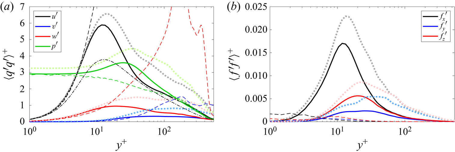
The variances of the state and forcing components are displayed in figure 14. Filtered DNS values (thick light dotted lines), true (continuous lines), white noise (dashed lines) and eddy-viscosity model (dash–dotted lines) estimates are provided in the figure. As the filtered DNS values are used, the variances are lower than those of the full DNS (reported in Morra et al. (Reference Morra, Nogueira, Cavalieri and Henningson2021)), but they are useful for comparison with the estimates, as both include the same wavenumbers. The variance of the estimates obtained using the true forcing statistics are close to the DNS values, with slight underestimations for $u^{\prime }$ and $p^{\prime }$ and more significant underestimations for $v^{\prime }$ and $w^{\prime }$, whereas comparisons with the white-noise forcing estimates are not as good. The eddy-viscosity model, for which only the streamwise velocity component results are shown, corrected the overshoot of white-noise forcing estimate but underestimates the variance values. Again, the peak error values for white-noise forcing far exceed the axes (2846 and 9.55 for $u^{\prime }$ and $w^{\prime }$, respectively). Two main factor contribute to the underestimation of the variance when employing the true statistics to build the transfer function. First, if a structure has no footprints on the wall, it cannot be estimated. Second, if there are more uncorrelated structures that contribute to the variance than there are sensors (2–3 in our case), not all of them will be properly estimated.

Figure 14.

Variance of filtered DNS and estimate data for $Re_{\tau } \approx 550$ and wall measurements of shear stress and pressure. See comments in the caption of figure 12. The thick light dotted lines correspond to DNS values. Continuous, dashed and dash–dotted lines denote estimates obtained with true forcing statistics, white-noise and the eddy-viscosity model, respectively.

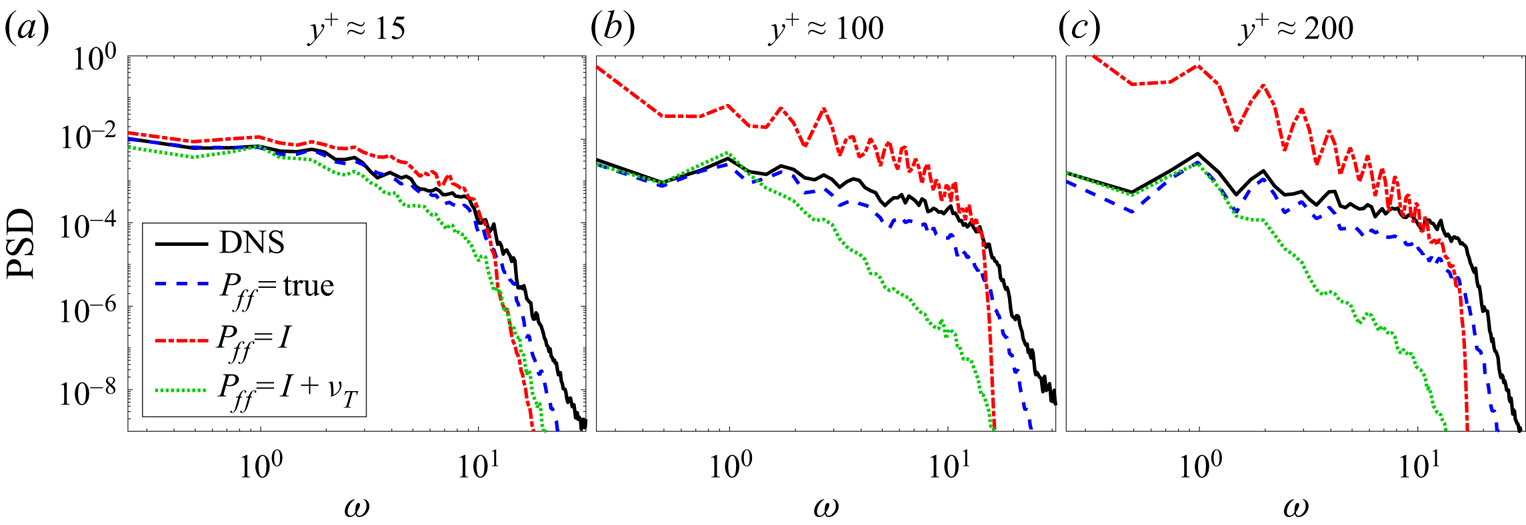
Figure 15 shows the PSD of the streamwise velocity as a function of non-dimensional frequency $\omega$ evaluated for $y^{+} \approx 15$, 100 and 200. The DNS results (continuous lines) and true (dashed lines), white (dash–dotted lines) and eddy-viscosity model (dotted lines) forcing estimates are displayed in the figure. Near the wall, the PSD of the estimates obtained using true forcing statistics is close to the DNS results, especially up to $\omega \approx 10$. The white-noise forcing assumption slightly overestimates the PSD at lower frequencies and for higher frequencies, i.e. $\omega \geq 12$, the spectral content is underestimated. When considering the white-noise estimate, the low- and high-frequency PSD levels are considerably overestimated and underestimated, respectively, for larger wall-normal distances. The eddy-viscosity model estimate achieves an intermediate performance, closer to the true-forcing-statistics assumption for lower frequencies and to the white-noise assumption for higher frequencies. This analysis corroborates the previous results of this section and shows that the resolvent-based estimator is best suited for low frequency flow dynamics. Results for other state components are qualitatively similar.

Figure 15.

Streamwise velocity PSD for $Re_{\tau } \approx 550$ and wall measurements of shear stress and pressure. Measurements taken for the probe located at $(x, z) = (0, 0)$ as a function of wall-normal direction $y^{+}$. Panels (a–c) are $y^{+} \approx 15$, 100 and 200, respectively. The frequency $\omega$ is non-dimensionalised in outer units.

3.5. Comparison between modelling strategies for the forcing

In the above sections, three different modelling strategies for the unknown forcing terms were studied, i.e. the true forcing statistics, obtained directly from the DNS, white-noise forcing and coloured noise based on an eddy-viscosity model. Table 3 summarises the main features of each of these strategies, focusing on the computational cost and estimation accuracy.

Table 3.

Summary of the cost and accuracy of the three forcing terms modelling strategies.

As the problem studied here has two homogeneous directions, estimates were obtained individually for each wavenumber pair, wall-normal discretisation and time step. The larger significant cost for this problem is constructing $\boldsymbol{\mathsf{P}}_{\boldsymbol{\mathsf{ff}}}$ from the DNS data using Welch's method. With this information, constructing the estimator (2.10) is very inexpensive, requiring only matrix multiplications of size $4 N_y$, and the convolutions (2.11)–(2.12) can be effectively computed using fast Fourier transforms. For an effective implementation of this procedure for large databases, we refer the reader to Martini et al. (Reference Martini, Jordan, Cavalieri, Towne and Lesshafft2020).

As shown in the previous subsections, the true forcing statistics provide greater accuracy compared with the other two forcing models. For near-wall structures, the estimate is very similar to the DNS when the true forcing is considered, closely followed by white-noise forcing. Interestingly, for near-wall structures, the white-noise forcing provided more accurate estimates than the eddy-viscosity model. On the other hand, estimates of large-scale structures are not as accurate, although the coloured forcing outperformed the other two models. The eddy-viscosity model provided better estimates than white-noise forcing for larger scale structures. The performance is nonetheless considerably worse than when true forcing statistics are used.

4.1. Overall comparison of estimation performance

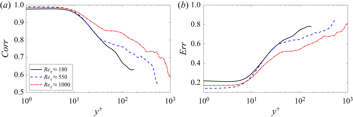
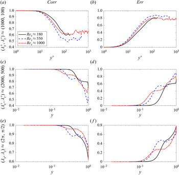
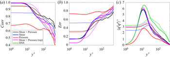
Figure 16 shows results of correlation ($Corr$, defined in (3.1)) and normalised r.m.s. error ($Err$, defined in (3.2)) for the streamwise velocity component for the three Reynolds numbers, and estimates obtained using true forcing statistics. In the figure, the continuous, dashed and dash–dotted lines denote the $Re_{\tau } \approx 180$, 550 and 1000 cases, respectively. Very close to the wall, the $Re_{\tau } \approx 550$ estimate achieves the highest correlation value, of approximately 0.99, followed by the $Re_{\tau } \approx 1000$ and 180 estimates, which have maximum correlation values of 0.98 and 0.97, respectively. The high correlations are almost constant up to $y^{+} \approx 7$ for all three Reynolds numbers. For higher distances, the correlation deteriorates for all cases. At the channel centre, the correlation decreases to approximately 0.6 for the $Re_{\tau } \approx 180$, 550 and 1000 estimates, respectively. Despite the decrease in correlation between estimates and DNS data, the values remain significant throughout the channel for all three Reynolds numbers. A collapse of correlations until the end of the buffer layer, at $y^{+} \approx 30$, is obtained for $Re_{\tau } \approx 180$ and 550 estimates. Similar trends as those observed in figure 16 were obtained for the other state components ($v$, $w$ and $p$).

Figure 16.

Streamwise velocity correlation (a) and error (b) evaluated for the probe at $(x,z) = (0,0)$. Estimates obtained using wall measurements of shear stress and true forcing statistics for $Re_{\tau } \approx$ 180, 550 and 1000.

Similar properties of the estimates can be inferred using the normalised r.m.s. error. Close to the wall, the lowest errors are observed for $Re_{tau} \approx 550$ (approximately 0.14), followed by $Re_{\tau }\approx 1000$ and 180 (0.17 and 0.22, respectively). The hierarchy of estimation performance for the r.m.s. normalised error metric is the same as that observed for the correlation metric, as well as the collapse of $Re_{\tau } \approx 180$ and 550 cases and the slope for the three cases in the $15 \leq y^+ \leq 35$ range. Moving towards the channel centre, the error metric deteriorates and is approximately 0.8 for the $Re_{\tau } \approx 180$, 550 and 1000 estimates, respectively. Again, similar trends for the other state components were obtained.

The overall correlation and error shown in figure 16 helps establish a Reynolds number trend, but there are differences in the wavenumbers retained in each database (presented in table 2), such that the range of wavenumbers may lead to differences in estimate accuracy. Moreover, the wavenumber spectra is known to display an increasing outer peak, related to large-scale structures, as the Reynolds number is increased (Smits et al. Reference Smits, McKeon and Marusic2011). In what follows we will assess the estimation accuracy for individual wavenumbers to better evaluate the Reynolds-number trend.

4.2. Estimation accuracy as a function of wavenumber

Normalised correlation and r.m.s. error metrics as a function of each wavenumber pair ($\alpha ,\beta$) and channel height $y$ can be obtained as

(4.1)\begin{equation} Corr(\alpha,y,\beta) = \frac{\displaystyle\int {q_{DNS}}\left(\alpha,y,\beta,t\right) {q_{est}^{*}}\left(\alpha,y,\beta,t\right) \textrm{d}t}{\sqrt{\displaystyle\int {{q_{DNS}}\left(\alpha,y,\beta,t\right)}^2 \,\textrm{d}t} \sqrt{\int {{q_{est}}\left(\alpha,y,\beta,t\right)}^2 \,\textrm{d}t}} {,} \end{equation}

and

(4.2)\begin{equation} Err(\alpha,y,\beta) = \frac{\sqrt{\displaystyle\int\sum_{i=1}^{3} \left|{q_{est}^i}\left(\alpha,y,\beta,t\right) - {q_{DNS}^i}\left(\alpha,y,\beta,t\right)\right|^2 \,\textrm{d}t}}{{\sqrt{\displaystyle\int \sum_{i=1}^{3} \left|{q_{DNS}^i}\left(\alpha,y,\beta,t\right)\right|^2 \,\textrm{d}t}}} {.} \end{equation}

The superscript $i$ in ${q^{i}}$, for $i = 1$, 2 and 3, denotes streamwise ($u^{\prime }$), wall-normal ($v^{\prime }$) and spanwise ($w^{\prime }$) velocity components, respectively. Note that instead of employing the probe at $(x,z) = (0,0)$, as in (3.1) and (3.2), the error and correlation curves obtained after (4.2) and (4.1) are functions of each wavenumber pair and wall-normal distance $y$. This error metric is the same as that employed by Illingworth et al. (Reference Illingworth, Monty and Marusic2018) and Oehler et al. (Reference Oehler, Garcia-Gutiérrez and Illingworth2018) to evaluate the performance of their estimator for each wavenumber.

Figure 17 shows correlation and normalised r.m.s. error for $({\lambda _{x}}^{+},{\lambda _{z}}^{+}) \approx (1000,100)$ (figure 17a,b), representative of near-wall structures, $({\lambda _{x}},{\lambda _{z}}) \approx (2{\rm \pi} ,{\rm \pi} /2)$ (figure 17e, f), representative of large-scale structures, and $({\lambda _{x}}^{+},{\lambda _{z}}^{+}) \approx (2000,500)$ (figure 17c,d), representative of intermediate-size structures, typical of a logarithmic layer if the Reynolds number is sufficiently high. For near-wall structures, correlation and error are approximately independent of the Reynolds numbers (especially the error) if wall-normal distance is scaled in inner units. On the other hand, the correlation and error results for the three Reynolds numbers do not collapse as well for the large-scale structures, but similar trends are observed if outer units are used to scale the wall-normal coordinate. This is in agreement with the expected scaling of buffer layer and large-scale structures in inner and outer units, respectively (Smits et al. Reference Smits, McKeon and Marusic2011).

Figure 17.

Streamwise velocity correlation (4.1, panels (a,c,e)) and error (4.2, panels (b,d, f)) evaluated for (a,b) $({\lambda _{x}}^{+},{\lambda _{z}}^{+}) \approx (1000,100)$, (c,d) $({\lambda _{x}}^{+},{\lambda _{z}}^{+}) \approx (2000,500)$ and (e, f) $({\lambda _{x}},{\lambda _{z}})\approx (2{\rm \pi} ,{\rm \pi} /2)$. Estimates obtained using wall measurements of shear stress and true forcing statistics for $Re_{\tau } \approx$ 180, 550 and 1000.

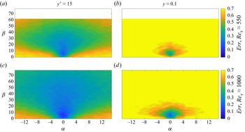
Figure 18 shows the normalised r.m.s. error, evaluated according to (4.2), for planes $y^+ \approx 15$ and $y \approx 0.1$, panels (a,c) and (b,d), respectively, and for the $Re_{\tau } \approx$ 550 and 1000 estimates, panels (a,b) and (c,d), respectively. In the plots, the contour scale is limited between 0 and 0.7, to enable a comparison with the plots by Illingworth et al. (Reference Illingworth, Monty and Marusic2018) and Oehler et al. (Reference Oehler, Garcia-Gutiérrez and Illingworth2018). For the $Re_{\tau } \approx$ 550 estimates, the maximum errors are approximately 0.68 and 0.86 for planes $y^+ \approx 15$ and $y \approx 0.1$, respectively, whereas for the $Re_{\tau } \approx$ 1000 estimates, the maximum errors are approximately 0.62 and 0.79 for planes $y^+ \approx 15$ and $y \approx 0.1$, respectively. The largest errors occur for $\beta \approx 0$ and high values of $\alpha$, i.e. structures that are long in the spanwise direction and thin in the streamwise direction. Elongated structures in the streamwise direction, with low $\alpha$, are more accurately estimated.

Figure 18.

Normalised r.m.s. error (4.2) as a function of $(\alpha ,\beta )$ for (a,c) $y^+ \approx 15$ and (b,d) $y \approx 0.1$. Panels (a,b) and (c,d) show results for $Re_{\tau} \approx 550$ and 1000, respectively. True forcing statistics and shear stresses on both walls were used to perform the estimates.

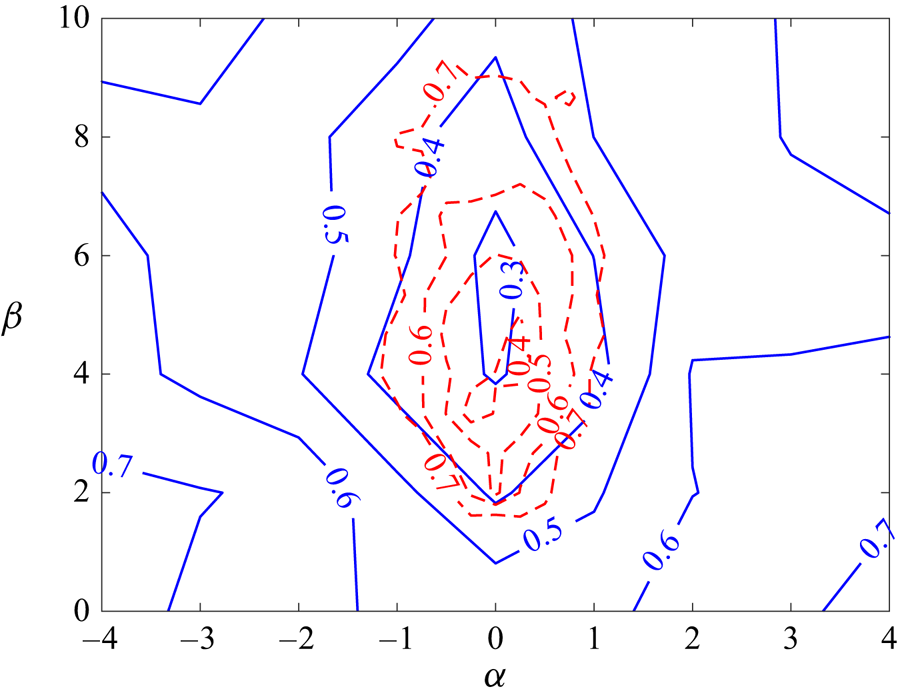
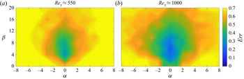
Illingworth et al. (Reference Illingworth, Monty and Marusic2018) employed a Kalman filter and observed the streamwise, wall-normal and spanwise velocity components at a wall-normal distance of $y^+ = 197$ as inputs, evaluating the normalised r.m.s. the error at the plane $y \approx 0.1$ ($y^+ = 100$ for the $Re_{\tau } = 1000$ channel considered in that work). The authors studied two estimators, the first based on the LNS equations with white-noise forcing, which showed a maximum error of 8.37, and the second including an eddy-viscosity model in the linear operator, which boosted the performance, displaying a maximum error of 1.07. Figure 19 contains a zoomed-in version of figure 18(c,d), restricting the wavenumber axes to match figure 4 of Illingworth et al. (Reference Illingworth, Monty and Marusic2018), i.e. $-8 \leq \alpha \leq 8$ and $0 \leq \beta \leq 20$. Figure 18(c,d) is equivalent to figure 4(a,b) in Illingworth et al. (Reference Illingworth, Monty and Marusic2018), i.e. both panels were obtained for $Re_{\tau } \approx$ 1000, with contour scale and wavenumber space limited to $Err \in [0,0.7]$, $\alpha \in [-8,8]$ and $\beta \in [0,20]$. The present estimates provide much lower errors than those obtained by Illingworth et al. (Reference Illingworth, Monty and Marusic2018), especially in the neighbourhood of $\alpha \approx 0$.

Figure 19.

Zoomed-in version of figure 18, with the normalised error for $y \approx 0.1$, restricting the wavenumber space to $-8 \leq \alpha \leq 8$ and $0 \leq \beta \leq 20$.

As discussed in the Introduction, the work by Oehler et al. (Reference Oehler, Garcia-Gutiérrez and Illingworth2018) is an extension of Illingworth et al. (Reference Illingworth, Monty and Marusic2018), including estimates performed at $Re_{\tau } = 2000$. The former authors also displayed normalised estimation error maps as a function of $(\alpha ,\beta )$ similar to those by Illingworth et al. (Reference Illingworth, Monty and Marusic2018) in their figure 6. Figure 20 shows a direct comparison between the normalised r.m.s. error as a function of wavenumber pair for the $Re_{\tau } \approx 1000$ estimate (continuous contours) and the results by Oehler et al. (Reference Oehler, Garcia-Gutiérrez and Illingworth2018) (dashed contours). The resolvent-based method provides superior estimates, with lower error values extending over a wider wavenumber range. The results in § 3 show that these lower errors are achieved here by incorporating forcing statistics taken from the DNS. However, care should be taken in these comparisons with Illingworth et al. (Reference Illingworth, Monty and Marusic2018) and Oehler et al. (Reference Oehler, Garcia-Gutiérrez and Illingworth2018) due to differences in the measurement plane and Reynolds number, respectively. Moreover, the procedure in Illingworth et al. (Reference Illingworth, Monty and Marusic2018) and Oehler et al. (Reference Oehler, Garcia-Gutiérrez and Illingworth2018) ensures a causal estimation, whereas the present estimates are not causal.

Figure 20.

Comparison between the normalised r.m.s. errors of the $Re_{\tau } \approx 1000$ estimate (blue continuous contours) and Oehler et al. (Reference Oehler, Garcia-Gutiérrez and Illingworth2018) results (red dashed contours), for estimates at $y = 0.1$ and 0.3. An average of $Err$ at the two heights was taken, following Oehler et al. (Reference Oehler, Garcia-Gutiérrez and Illingworth2018).

4.3. Maximum observed height

The trend of accuracy loss far from the wall can be quantified by defining a maximum observed distance. This distance is here defined as the position for which $Err(\alpha ,{y_{obs}},\beta ) \leq 0.5$. Figure 21 shows contour maps of the observable height in inner units, i.e. $y_{obs}^{+}$, measured from the channel wall, for the three studied Reynolds numbers. This 0.5 maximum normalised error criterion and contour levels of $y^{+} = 15$, 30, 50, 100 and 200 were employed to obtain the maps shown in figure 21. Smaller structures, of small wavelength pair (${\lambda _{x}}^{+},{\lambda _{z}}^{+}$), can only be estimated near the wall. Far from the wall, only the larger structures are observed. This behaviour is consistently observed for the three Reynolds numbers. These results corroborate the snapshot reconstructions and power spectra previously addressed, e.g. figure 7, where the small structures that are present in the DNS snapshot at a distance of $y^{+} \approx 200$ could not be properly estimated. As the Reynolds number is increased, the emergence of larger-scale structures at higher $y^+$ is captured by the estimation, with large wavelengths observed at logarithmic-layer heights $y^+ \approx 100$ and 200.

Figure 21.

Observed height ($y_{obs}^{+}$) maps for the three Reynolds numbers. Estimates obtained using wall measurements of shear stress for $Re_{\tau } \approx$ 180, 550 and 1000.