2 Theory

In this section we present the theoretical background for our numerical results in this paper, including the statistics of the displacement of single molecules (§ 2.1), the separation between pairs of molecules at specified initial separations in both forward and backward reference frames (§ 2.2), and the connection between Lagrangian and Eulerian results for passive scalar mixing (§ 2.3). For stationary turbulence we expect the theoretical results derived by Saffman (Reference Saffman1960) for one-molecule statistics to hold equally well for both forward and backward dispersion. However, for pairs, it is important to make the distinction. It is well known that backward relative dispersion at intermediate times is stronger than forward dispersion (Sawford et al. Reference Sawford, Yeung and Borgas2005; Berg et al. Reference Berg, Luthi, Mann and Ott2006). There has been, in fact, considerable recent interest in backward dispersion of fluid particles (Jucha et al. Reference Jucha, Xu, Pumir and Bodenschatz2014; Buaria et al. Reference Buaria, Sawford and Yeung2015) as well as theoretical work on molecular trajectories (Eyink Reference Eyink2011; Benveniste & Drivas Reference Benveniste and Drivas2014). However, current knowledge of molecular path statistics especially with regard to their Schmidt number dependence and connection to Eulerian passive scalar statistics is still limited.

3 Numerical approach and database

We have performed simulations of stationary isotropic turbulence over a range of Reynolds numbers. The Eulerian velocity and scalar fields are computed using a pseudo-spectral approach in space and a second-order Runge–Kutta integration in time. Stationarity in the velocity field is achieved by maintaining (Donzis & Yeung Reference Donzis and Yeung2010) the energy spectrum in the lowest few wavenumber shells at values suggested by long-time averages derived from previous simulations which used stochastic forcing (Eswaran & Pope Reference Eswaran and Pope1988). For scalar fields the fluctuations are initially absent but subsequently generated by a uniform mean gradient. Although the forcing scheme employed tends to minimize temporal oscillations of the kinetic energy and dissipation rate, statistics in specific directions can still vary significantly at a given time instant. In order to minimize limitations in statistical sampling, for each value of $Sc$ we simulate and subsequently average over results for three scalars with $\boldsymbol{{\rm\nabla}}{\it\Phi}$ in different coordinate directions.

Molecules are tracked by integrating (1.1) using an extension of a parallelized particle-tracking algorithm used recently for fluid particles (Buaria et al. Reference Buaria, Sawford and Yeung2015). To advance from time $t_{n}$ to $t_{n+1}=t_{n}+{\rm\Delta}t$ we calculate the predictor step estimate of the new position $\boldsymbol{x}^{m}(t_{n+1})$ by the formula

where $\boldsymbol{Z}$ is a standardized Gaussian random variable in 3D, and the Wiener process increment is implemented as $\text{d}\boldsymbol{W}=\sqrt{{\rm\Delta}t}~\boldsymbol{Z}$ . The end result, after the corrector step, is

The fluid velocities at the two molecular positions shown in (3.2) are calculated by cubic-spline interpolation (Yeung & Pope Reference Yeung and Pope1988). This scheme is strong order $1/2$ and weak order 1 (Kloeden & Platen Reference Kloeden and Platen1992). However, in contrast to Eulerian simulations, no special numerical constraints arise for the time step or grid spacing at either very low or very high Schmidt number (Donzis et al. Reference Donzis, Sreenivasan and Yeung2010; Yeung & Sreenivasan Reference Yeung and Sreenivasan2014), although it is obviously important to have a substantial number of molecules for statistical sampling. This approach is similar to the thermal marker technique of Papavassiliou & Hanratty (Reference Papavassiliou and Hanratty1995).

To obtain both forward and backward displacement statistics, we use our recently developed postprocessing approach (Buaria et al. Reference Buaria, Sawford and Yeung2015). While single-molecule statistics are relatively simple to obtain, two-molecule statistics require a careful approach in forming pairs of desired initial separation from the entire population. For a given trajectory extending from $t=0$ to $t=T$ , the initial separation for forward pairs is simply $r_{0}=|\boldsymbol{r}(t=0)|$ , whereas for backward pairs the initial separation is defined as $r_{0}=|\boldsymbol{r}(t^{\prime }=0)|$ , where $t^{\prime }=T-t$ is the backward time. Thus, forward and backward statistics are compared using the properties of $\boldsymbol{r}(t)$ and $\boldsymbol{r}(t^{\prime })$ . However, since the turbulence is stationary, the statistics evaluated at any time $t^{\prime }$ are equivalent to those evaluated at time $-t$ . Henceforth, for convenience, we will use $t$ to represent both forward and backward times, unless specified otherwise. Since pairs are formed from a population of many millions, samples of $r_{0}$ vary continuously over a wide range and are (see § 5) sorted into bins of finite width. This method allows us to compute the backward statistics without the need to store numerous time-resolved snapshots of the velocity field, which would be extremely memory-intensive, especially as the Reynolds number increases. Since final-time positions are not prescribed, we have no samples of initially coincident molecular pairs in the backward frame, and pairs of small $r_{0}$ are correspondingly fewer in number. However, in most cases adequate sampling is achieved for pairs of initial separation down to as small as ${\it\eta}/4$ , which, as seen later in § 6, is generally sufficiently small as an approximation to $r_{0}=0$ . More details about the methodology can be found in Buaria et al. (Reference Buaria, Sawford and Yeung2015).

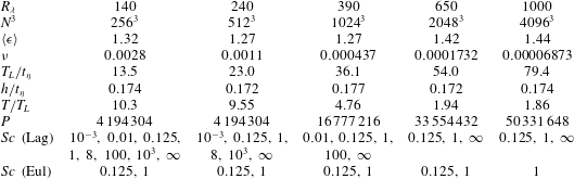
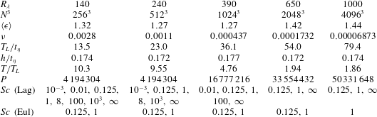
Table 1 gives a summary of the database used in the current work along with the main simulation parameters. In all cases the solution domain is of length $2{\rm\pi}$ on each side, and the grid spacing is approximately twice the Kolmogorov length scale ${\it\eta}$ . As mentioned earlier, the forcing scheme used (Donzis & Yeung Reference Donzis and Yeung2010) tends to limit the variations in kinetic energy and mean dissipation rate, and thus both ${\it\eta}$ and $t_{{\it\eta}}$ can be taken as constant throughout each simulation. Most of the simulation parameters are the same as reported in our recent work (Buaria et al. Reference Buaria, Sawford and Yeung2015) focused on fluid particle pairs, except that the time span of both Eulerian and Lagrangian simulation at $R_{{\it\lambda}}=650$ and 1000 is limited by computational expense. In the smaller simulations we have tracked molecules at several values of the Schmidt number spanning many decades. For time-dependent Eulerian scalar fields we have limited ourselves to $Sc=0.125$ and 1 (and only the latter in the more expensive $4096^{3}$ simulation).

Table 1.

Parameters of the simulations performed: the Taylor-scale Reynolds number ( $R_{{\it\lambda}}$ ), the number of grid points ( $N^{3}$ ), the mean dissipation rate ( $\langle {\it\epsilon}\rangle$ ), the kinematic viscosity ( ${\it\nu}$ ), the ratio of the Lagrangian integral time scale ( $T_{L}$ ) to the Kolmogorov time scale ( $t_{{\it\eta}}$ ), the output time interval ( $h$ ) in Kolmogorov scales, the time span of the simulation ( $T$ ) in integral time scales, the number of molecules ( $P$ ) tracked for each value of the Schmidt number ( $Sc$ ) and the values of $Sc$ computed for each case in both the Lagrangian (Lag) and the Eulerian (Eul) part. The case $Sc=\infty$ corresponds to fluid particles.

4 Single-molecule statistics

Single-molecule statistics (where each molecule is an independent sample) provide a basic characterization of molecular trajectory properties and are also related to the production of scalar variance (§ 2.3). In this section we do not differentiate between forward and backward results, since in stationary turbulence these statistics are equivalent.

Figure 1.

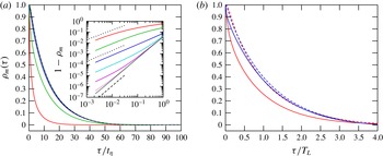
Substance autocorrelation: (a) as a function of the non-dimensional time lag ( ${\it\tau}/t_{{\it\eta}}$ ) for $R_{{\it\lambda}}=140$ and, from bottom to top, for $Sc=0.001$ (red), $0.01$ (green), $0.125$ (blue), $1$ (cyan), 8 (magenta), 100 (pink), 1000 (dark green) and $\infty$ (dashed black); data for $Sc=100$ and 1000 are almost indistinguishable from $Sc=\infty$ ; the inset shows $1-{\it\rho}_{m}$ on log–log scales with $Sc$ increasing downwards, with dotted and dashed straight lines indicating slopes $1$ and $2$ respectively; (b) versus the time lag scaled by $T_{L}$ , for $Sc=0.01$ (solid) and $\infty$ (dashed), at $R_{{\it\lambda}}=140$ (red) (lower lines) and $390$ (blue) (upper lines).

As suggested in § 2.1, the first quantity to examine is the substance autocorrelation, ${\it\rho}_{m}({\it\tau})$ , which by stationarity is an even function of the time lag ( ${\it\tau}$ ). Figure 1 shows, as a function of time lag, (a) ${\it\rho}_{m}({\it\tau})$ for a range of $Sc$ at given $R_{{\it\lambda}}$ , and (b) data for a range of $R_{{\it\lambda}}$ at given $Sc$ . The case $Sc=\infty$ corresponds to fluid particles. In (a), with $R_{{\it\lambda}}$ held fixed at 140, as $Sc$ decreases, we observe that the autocorrelation drops off to zero faster with time. This faster decorrelation at decreasing $Sc$ is expected, because Brownian motion contributions to the displacements at successive time instants are independent and uncorrelated, and these contributions become stronger at higher molecular diffusivity. However, the departure from the fluid particle case is substantial only for $Sc\ll 1$ , showing that the effects of molecular diffusion are weak compared with turbulent transport unless $Sc$ is less than unity.

It is well understood that since the velocity of a fluid particle is differentiable in time, the fluid particle velocity autocorrelation ${\it\rho}_{L}({\it\tau})$ has a parabolic decay near ${\it\tau}=0$ , i.e.

where ${\it\lambda}_{t}$ is the Taylor time scale related to the acceleration variance ${\it\sigma}_{a}^{2}$ as $\sqrt{2}{\it\sigma}_{u}/{\it\sigma}_{a}$ . By expressing ${\it\sigma}_{a}$ in Kolmogorov variables and substituting this in (2.6) we obtain

where $a_{0}$ is the Kolmogorov-scaled acceleration variance (which is known to increase with Reynolds number as a result of intermittency (Yeung et al. Reference Yeung, Pope, Lamorgese and Donzis2006)). The linear term in (4.2) will dominate if ${\it\tau}/t_{{\it\eta}}\ll a_{0}^{2}Sc$ , which is more easily satisfied at low $R_{{\it\lambda}}$ and low $Sc$ . To examine this behaviour, in the inset in figure 1(a) we show $1-{\it\rho}_{m}$ versus ${\it\tau}/t_{{\it\eta}}$ on log–log scales. The approach to linear behaviour at small time lags is very readily seen for $Sc<1$ . For $Sc>1$ there is a range of times $a_{0}^{-2}Sc^{-1}\ll t/t_{{\it\eta}}\ll 1$ over which the quadratic term in (4.2) dominates. Thus, for $Sc>1$ , we can observe that the curves nearly overlap (as the quadratic term is independent of $Sc$ ) and display slope 2 at early time lags.

The effect of the Reynolds number on the Schmidt number dependence is seen in figure 1(b), which shows the substance autocorrelation for $Sc=0.01$ and the fluid particle velocity autocorrelation (i.e. $Sc=\infty$ ). The difference between the two solid lines is substantial, showing that at fixed $Sc$ the decorrelation with increasing time lag occurs more slowly when the Reynolds number increases. However, it is also clear that at higher Reynolds number the difference between the solid and dashed blue (upper) lines is weak, which indicates that the sensitivity to $Sc$ is much diminished as the Reynolds number increases.

Table 2.

Lagrangian integral time scale for molecular trajectories.

The areas under the curves in figures 1(a) and 1(b) are (based on the normalization chosen) equal to the ratios $T_{m}/t_{{\it\eta}}$ and $T_{m}/T_{L}$ respectively. These ratios are themselves related through the factor $T_{L}/t_{{\it\eta}}$ , which increases with the Reynolds number. Table 2 shows the variation of $T_{m}/T_{L}$ with $Sc$ at $R_{{\it\lambda}}$ up to 390. (At $R_{{\it\lambda}}$ 650 and 1000 the simulation time $T/T_{L}$ is too short to estimate $T_{m}/T_{L}$ reliably.) It can be seen that $T_{m}/T_{L}$ is relatively low for $Sc\ll 1$ and approaches unity as $Sc$ increases. In addition, as the Reynolds number increases, $T_{m}/T_{L}$ at a given $Sc$ becomes closer to unity. This is consistent with the fact that as the Reynolds number increases the influence of molecular diffusion also becomes very weak. However, for finite Reynolds number, the effects of molecular diffusion must be taken into account, especially if $Sc$ is low and $R_{{\it\lambda}}$ is modest.

Figure 2.

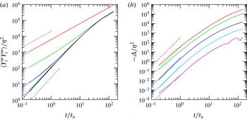
(a) Single-molecule Kolmogorov-scaled mean-square displacement at $R_{{\it\lambda}}=140$ , for $Sc=0.001$ (red), $0.01$ (green), $0.125$ (blue), $1$ (cyan), $8$ (magenta), $100$ (orange) and $1000$ (black), increasing from top to bottom (the last three cases being virtually indistinguishable). The dashed colour lines are the corresponding small-time results given by (2.7). The dotted black lines are for slopes 1 and 2. (b) The negative of the interaction term given by (2.4), scaled by Kolmogorov variables, for $R_{{\it\lambda}}=140$ and $Sc=0.001$ , 0.01, 0.125, 1 and 8 (same colours as in (a)), increasing from top to bottom. The dashed colour lines represent Saffman’s small-time results given by (2.8).

Figure 2 shows (a) the mean-square displacement and (b) the magnitude of the interaction term (defined in (2.4)), both normalized by Kolmogorov variables. As a result of molecular diffusion, the behaviour of the mean-square displacement at small times, as given by (2.7), is very different depending on the Schmidt number. For sufficiently small times $t/t_{{\it\eta}}\ll Sc^{-1}R_{{\it\lambda}}^{-1}$ the linear diffusion term dominates, as is readily seen for $Sc<1$ in figure 2(a), where $Sc$ is varied over a wide range at fixed $R_{{\it\lambda}}$ . For large $Sc$ and/or large $R_{{\it\lambda}}$ this linear growth is restricted to very small times and there is a range of times $Sc^{-1}R_{{\it\lambda}}^{-1}\ll t/t_{{\it\eta}}\ll 1$ over which the quadratic ballistic term dominates. This is readily seen in the collapse of curves for $Sc>1$ onto the fluid particle result for $Sc=\infty$ . At large times, all curves approach a diffusive regime where the growth of the mean-square displacement is linear, as given by (2.9). However, the curve for $Sc=0.001$ lies far above all the others, which is because in this case the diffusivity is so high that the second term in (2.9) dominates. By using ${\it\sigma}_{u}^{2}T_{m}={\it\kappa}_{t}$ as defined earlier, the mean-square displacement equals $6({\it\kappa}_{t}+{\it\kappa})t$ , such that the slope in the large-time limit is determined by the additive effect of the turbulent and molecular diffusivities. The Schmidt number dependence at other Reynolds numbers also follows similar trends, but at higher $R_{{\it\lambda}}$ generally a lower $Sc$ is needed for molecular diffusion to be dominant.

A more sensitive test of Schmidt number effects is to plot the interaction term given by (2.4), which explicitly quantifies the effects of molecular diffusion on turbulence. In figure 2(b) it can be seen that, although there is some numerical noise resulting from taking differences between small values which are very close to each other, the agreement with (2.9) is good for moderate and high $Sc$ . However, with decreasing $Sc$ the DNS data fall increasingly below the theory. This is because, as noted before, (2.8) holds only at times $t/t_{{\it\eta}}\ll Sc$ , which is not satisfied in the data range of figure 2(b).

Figure 3.

Variation of the molecular integral time scale with respect to the Lagrangian time scale as a function of $Sc$ for $R_{{\it\lambda}}=140$ (circles, in red), $240$ (triangles, in green) and $390$ (squares, in blue). The open and closed symbols represent estimates based on the substance autocorrelation and the interaction term respectively. The dashed lines are at slope $-1$ .

On the other hand, at large times, the interaction term is given by (2.10), in which the relative magnitudes of the integral time scales $T_{m}$ and $T_{L}$ are important. In figure 3 we show data for $1-T_{m}/T_{L}$ versus $Sc$ , which provides a test for the functional form suggested in (2.13), with each dashed line corresponding to a different value of the parameter $a$ therein. At high $Sc$ , or at moderate $Sc$ at high $R_{{\it\lambda}}$ , $T_{m}$ becomes very close to $T_{L}$ and the quantity $1-T_{m}/T_{L}$ can become unreliable, or even spuriously negative, especially if $T_{m}$ or $T_{L}$ is affected by limitations such as the length of the simulation. As a result, some data points corresponding to cases listed in table 2 are not shown in this figure which is drawn on logarithmic scales. Nevertheless, good agreement with the $Sc^{-1}$ dependence of Saffman’s theoretical result is observed over a range of moderate Schmidt numbers, but with the parameter $a$ dependent on the Reynolds number. At very low $Sc$ , the discrepancy between theory and DNS is substantial, which is not surprising since physically both $T_{m}$ and $T_{L}$ must be non-negative with $T_{m}\leqslant T_{L}$ , so $1-T_{m}/T_{L}\leqslant 1$ .

5 Statistics of molecule pairs

In this section we present results for the forward and backward dispersion of molecular pairs. Since the turbulence is isotropic, the dependence on the initial separation vector is through its magnitude ( $r_{0}$ ) only. The statistics of molecule pairs are extracted using the same approach as our recent work on fluid particle pairs (Buaria et al. Reference Buaria, Sawford and Yeung2015), where samples of a continuous variation of $r_{0}$ are sorted into finite bins of logarithmic spacing. To enhance the sampling without sacrificing resolution in $r_{0}$ , we choose overlapping bins within a factor of four, defined as $2^{i-3}\leqslant r_{0}/{\it\eta}\leqslant 2^{i-1}$ for $i=0,1,2,3,\ldots$ onwards. To identify a bin, we use $\tilde{r}_{0}/{\it\eta}$ , which is the geometric mean between its lower and upper bounds, normalized by the Kolmogorov scale, i.e. $\tilde{r}_{0}/{\it\eta}=2^{i-2}$ for $i=0,1,2,3,\ldots$ onwards. Consequently, all of the pair statistics reported here are averages over the sample of initial separations in each bin, and so are reported as functions of $\tilde{r}_{0}$ rather than the random variable $r_{0}$ . Earlier studies focused on fluid particles (Sawford et al. Reference Sawford, Yeung and Borgas2005; Berg et al. Reference Berg, Luthi, Mann and Ott2006) have shown that backward dispersion is similar to forward dispersion at both very short and very long times but stronger at intermediate times. More recently, it has been recognized that (Jucha et al. Reference Jucha, Xu, Pumir and Bodenschatz2014; Buaria et al. Reference Buaria, Sawford and Yeung2015) the forward and backward dispersion do differ at early but finite times, at a rate that grows as $t^{3}$ , which could be overlooked if only the leading $t^{2}$ terms in the Taylor-series expansions for both forward and backward mean-square relative displacement were retained.

Figure 4.

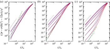
Compensated mean-square relative displacement of molecule pairs as a function of forward time (solid lines, in red) and backward time (dashed lines, in blue), scaled by Kolmogorov variables, at $R_{{\it\lambda}}=140$ for $Sc=0.01$ (a), $1$ (b) and $100$  (c). The green dashed lines represent the Saffman $t^{3}$ small-time limit. The value of $\tilde{r}_{0}/{\it\eta}$ (1/4, 1, 4, 16, 64) increases from bottom to top. (In (a) the lines for $\tilde{r}_{0}/{\it\eta}=1/4$ and $1$ are virtually indistinguishable, whereas in (b) the $\tilde{r}_{0}/{\it\eta}=1/4$ data coincide with the long-dashed line in green at small times.) The black dotted lines indicate a slope of  $2$ .

An important question in this section is how molecular diffusion affects the behaviour of the mean-square relative displacement, $\langle |\boldsymbol{r}(t)-\boldsymbol{r}(0)|^{2}\rangle$ . In view of the structure of (2.17)–(2.18), it is convenient to separate out the linear diffusive term, which could become large at low $Sc$ and obscure other effects of interest. Accordingly, in figure 4 we show the evolution of the mean-square relative displacement compensated for the direct effect of molecular diffusion, i.e. $(\langle |\boldsymbol{r}(t)-\boldsymbol{r}(0)|^{2}\rangle -12{\it\kappa}t)/{\it\eta}^{2}$ , at three different Schmidt numbers with fixed $R_{{\it\lambda}}=140$ . On the scales of this figure, forward and backward dispersion generally agree closely at both small and large times. At large times ( $t\gg T_{m}$ ), the curves for all values of $\tilde{r}_{0}$ are also seen to converge towards a linear diffusive limit, as given by (2.19). However, at very low $Sc$ (0.01 or lower), where molecular diffusion is dominant, the differences between forward and backward dispersion are small even at intermediate times. This is consistent with the results of Sawford et al. (Reference Sawford, Yeung and Borgas2005), who showed that forward and backward dispersion would be equivalent if the velocity field were Gaussian. As $Sc$ decreases, Brownian motion contributions (which are Gaussian) are more prominent. Approach to the large-time diffusive limit also occurs earlier for such small $Sc$ since the ratio $T_{m}/T_{L}$ (and hence $T_{m}/t_{{\it\eta}}$ ) decreases with decreasing $Sc$ .

The nature of the behaviour at early times in figure 4 is sensitive to both the initial separation and the Schmidt number. If $\tilde{r}_{0}$ is large, then unless $Sc$ is extremely small, the early-time growth is quadratic, as explained by (2.18). The lines for large $\tilde{r}_{0}$ are also closer to each other since the Eulerian structure functions increase monotonically with $\tilde{r}_{0}$ until they become constant at large $\tilde{r}_{0}$ . However, as discussed in relation to (2.17), if $\tilde{r}_{0}$ is small, the early-time behaviour depends strongly on $Sc$ , being cubic for ${\tilde{r}_{0}}^{2}/{\it\eta}^{2}\ll Sc^{-1}t/t_{{\it\eta}}$ with $t/t_{{\it\eta}}\ll \min (1,Sc)$ and quadratic for $t/t_{{\it\eta}}\ll Sc(\tilde{r}_{0}/{\it\eta})^{2}$ . Thus, in the data at $Sc=0.01$ , for $\tilde{r}_{0}/{\it\eta}\rightarrow 0$ we see a convergence to a stronger than quadratic dependence on time, but the times shown are too large for the Saffman $t^{3}$ behaviour to be observed. For $Sc=1$ , the data for $\tilde{r}_{0}/{\it\eta}=1/4$ converge to the Saffman result for both forward and backward dispersion. Finally, for $Sc=100$ , much smaller values of $\tilde{r}_{0}/{\it\eta}$ are needed to observe the Saffman result; instead, the ballistic $t^{2}$ behaviour is observed.

Figure 5.

Forward (a,c) and backward (b,d) CLS of mean-square separation, defined by (5.1), at $R_{{\it\lambda}}=390$ (dotted), $650$ (dashed) and $1000$ (solid) for $Sc=0.125$ (a,b) and $1$ (c,d). The initial separations are $\tilde{r}_{0}/{\it\eta}=2$ (red), $4$ (green), $8$ (blue) and $16$ (black) (right to left at large times). The horizontal dotted lines are drawn for reference at the heights $0.56$ (forward) and 1.57 (backward) for $Sc=0.125$ , $0.55$ (forward) and 1.53 (backward) for $Sc=1$ .

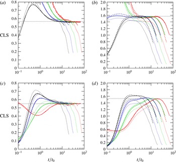
The most important dynamical issue at high Reynolds number is, of course, the possibility of Richardson scaling at intermediate times, as defined by (2.20). An effective way to characterize the scaling behaviour is to calculate the so-called cubed-local slope (CLS) (Sawford et al. Reference Sawford, Yeung and Hackl2008),

If a well-defined Richardson scaling range is present, then the plot of the CLS versus $t/t_{0}$ will show a plateau at height equal to Richardson’s constant, over a range of $\tilde{r}_{0}$ and in the range $(t_{{\it\eta}},t_{0},t_{{\it\kappa}})\ll t\ll T_{m}$ . In figure 5 we show data at the three highest Reynolds numbers for $Sc=0.125$ and $1$ , for four values of $\tilde{r}_{0}/{\it\eta}$ . In general, there is clear evidence for Richardson scaling, at slightly different plateau heights, for all cases shown, while (as for fluid particles) the Richardson constant for backward dispersion is higher. For the forward case of $Sc=0.125$ , as $R_{{\it\lambda}}$ increases, the plateau indicating Richardson scaling shifts down from 0.59 at $R_{{\it\lambda}}=390$ to 0.56 at $R_{{\it\lambda}}=650$ and $R_{{\it\lambda}}=1000$ . For $Sc=1$ , the data for $R_{{\it\lambda}}=650$ and $1000$ overlap almost perfectly with each other, indicating a very robust scaling, with the Richardson constant being $0.55$ , a little lower than the value of 0.56 for $Sc=0.125$ .

Figure 6.

Forward (a) and backward (b) CLS at $R_{{\it\lambda}}=1000$ for $Sc=0.125$ (solid), $1$ (dashed) and $\infty$ (dotted) for the same initial separations as figure 5. The horizontal dotted lines are drawn for reference at the heights 0.55 and 0.56 for forward, 1.53 and 1.57 for backward.

Table 3.

Forward and backward Richardson constants as estimated from the CLS plots for various $R_{{\it\lambda}}$ and $Sc$ . The data for $Sc=\infty$ are the same as those reported in Buaria et al. (Reference Buaria, Sawford and Yeung2015).

For backward dispersion, the convergence towards Richardson scaling is not as strong as for forward dispersion, especially at $Sc=1$ , but is still clearly evident. For $Sc=0.125$ , as $R_{{\it\lambda}}$ increases from 390 to 1000, there is a clear trend, with plateaus at $1.41$ , $1.55$ and $1.57$ . For $Sc=1$ , the plateaus tend to be defined by the decreasing trends in the peak values with decreasing $\tilde{r}_{0}$ , towards coincident values for $\tilde{r}_{0}/{\it\eta}=2$ and 4, rather than as an extended plateau for any one value of $\tilde{r}_{0}$ . These coincident values are $1.32$ , $1.50$ and $1.53$ for $R_{{\it\lambda}}=390$ , 650 and 1000 respectively.

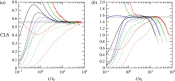
While figure 5 shows the Reynolds-number dependence at fixed Schmidt numbers, it is also useful to examine the Schmidt-number dependence of the CLS at the highest available $R_{{\it\lambda}}$ , including the case of $Sc=\infty$ (where we used fluid particle results given in Buaria et al. (Reference Buaria, Sawford and Yeung2015)). Figure 6 shows such data at $R_{{\it\lambda}}=1000$ for $Sc=0.125$ , 1 and $\infty$ . For forward dispersion (a), the curves for $Sc=1$ and $\infty$ essentially coincide at a plateau at height 0.55, a little lower than the plateau at 0.56 for $Sc=0.125$ . This suggests that the Richardson constant inferred here is well converged with respect to $Sc$ even if a weak decrease with $Sc$ may still persist. For the backward case (b), the dependence on $Sc$ is more visible, with the curves for $Sc=0.125$ plateauing at 1.57, which is slightly above the value of 1.53 for $Sc=1$ . For $Sc=\infty$ , the trends with both $\tilde{r}_{0}/{\it\eta}$ and $R_{{\it\lambda}}$ suggest a best estimate of $1.5$ for the backward Richardson constant (Buaria et al. Reference Buaria, Sawford and Yeung2015). This value corresponds to the short plateau for $\tilde{r}_{0}/{\it\eta}=8$ in figure 6. This again suggests that an even higher $R_{{\it\lambda}}$ is required to reach the asymptotic state for backward dispersion, at which the backward Richardson constant would also become independent of $Sc$ .

A summary of our estimates for both forward and backward Richardson constants is given in table 3. There are systematic trends with respect to both the Schmidt number and the Reynolds number, and clear convergence with both increasing $Sc$ at fixed $R_{{\it\lambda}}$ and vice versa. The trends are also consistent with the work of Eyink (Reference Eyink2011), who estimated the forward and backward constants to be 0.64 and 1.35 respectively using DNS results on stochastic tracers with zero initial separation for $Sc=1$ at $R_{{\it\lambda}}=433$ , and that of Benveniste & Drivas (Reference Benveniste and Drivas2014), who reported the backward constant to be 1.33 using the same database as Eyink (Reference Eyink2011). Thus, the overall conclusion is that both Schmidt-number and Reynolds-number effects on the value of Richardson’s constant (forward and backward) are weak, and that the values inferred here are consistent with those reported earlier for fluid particles (0.55 and 1.5 for forward and backward respectively, as shown in table 3 for $Sc=\infty$ ).

The general appearance of figures 5 and 6 bears several similarities to our recent analysis of Richardson scaling for fluid particles (Buaria et al. Reference Buaria, Sawford and Yeung2015). However, the scaling for molecules appears to be more robust. One possible explanation is that as a pair of molecules moves under the combined effects of turbulence and molecular diffusion, its memory of initial separation is lost faster than for fluid particles. If the Schmidt number is not too low, this effect may result in an early onset of a wider inertial range, with a wider plateau. While $Sc\sim O(1)$ produces a more robust Richardson scaling, for $Sc\ll 1$ molecular diffusion may be so strong that the nature of the dispersion becomes increasingly similar to pure Brownian motion, which deviates strongly from inertial range scaling. A complete absence of Richardson scaling is indeed found for our CLS data at $Sc=0.01$ and 0.001 (not shown), although at higher Reynolds numbers this behaviour would require increasingly lower Schmidt numbers.

Some authors (Eyink Reference Eyink2011; Benveniste & Drivas Reference Benveniste and Drivas2014) have argued that Richardson scaling is also supported by a collapse of results for the separation PDF onto the Richardson similarity form (Richardson Reference Richardson1926; Sawford et al. Reference Sawford, Yeung and Borgas2005). In fact, this collapse occurs over only a limited range of scales ( $r/\langle r^{2}\rangle ^{1/2}\leqslant 2$ ), and on larger scales there is no collapse (Buaria et al. Reference Buaria, Sawford and Yeung2015). Our results for molecular trajectories, not shown here, are consistent with those of Buaria et al. (Reference Buaria, Sawford and Yeung2015). This is not necessarily evidence for a failure of Richardson scaling, but rather shows that the assumption underlying the particular similarity form proposed by Richardson, namely that relative dispersion is described by a diffusion equation, is not satisfied.

The results of §§ 4 and 5 have provided reliable information on one- and two-molecule statistics over a Reynolds- and Schmidt-number range considerably wider than previously reported in the literature. In the next section we use these results to address turbulent mixing in a Lagrangian frame.

6 Lagrangian description of scalar mixing

In this section we use the results for displacement statistics given in earlier sections to derive scalar field statistics from a Lagrangian perspective. Comparisons with Eulerian results are made only for $Sc=0.125$ and $1$ , since higher or lower $Sc$ require more computational resources. As derived earlier in § 2.2, the scalar production and dissipation can be written in terms of displacement statistics for single molecules and pairs of molecules, as given by (2.30) and (2.29) respectively. However, both of these expressions involve numerical differentiation and subtraction between terms that may be very close to each other, especially for moderate and low $Sc$ . To avoid numerical inaccuracies caused by these issues we derive alternative formulae in appendix B. We compute the scalar production and dissipation terms using the expressions

where $u_{i}$ is the fluid velocity at the molecular position and $u_{i}^{(r)}$ is the relative fluid velocity between two molecules. In addition, stationarity allows us to replace (6.2) by

where $t^{\prime }=T-t$ , and conditioning on properties at the fixed final time ( $T$ ) of the simulations is more readily implemented. However, as seen later, (2.30) and (2.29) are still useful from a theoretical perspective.

Figure 7.

Non-dimensional scalar production as obtained from Lagrangian (solid lines) and Eulerian (dotted black lines) approaches, at $R_{{\it\lambda}}=140$ (red), $240$ (green), $390$ (blue), $650$ (cyan) and $1000$ (magenta), increasing from bottom to top. Panels (a) and (b) show data for $Sc=1/8$ and $1$ respectively. The Eulerian result at $R_{{\it\lambda}}=1000$ is given only for $Sc=1$ .

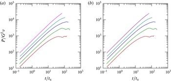
Figure 7 shows results for the scalar production normalized in the form $P/G^{2}{\it\nu}$ , for $Sc=1/8$ and 1, as the Reynolds number is varied from 140 to 1000. Excellent agreement is observed between the Lagrangian results (calculated from (2.30) and (6.1)) and the Eulerian result (dotted black lines) $P=-2\langle \boldsymbol{u}{\it\phi}\rangle \boldsymbol{\cdot }\boldsymbol{{\rm\nabla}}{\it\Phi}$ (§ 2.3), which is ensemble averaged over mean gradients aligned with each of the three coordinate axes. The normalization chosen allows the small-time results to be written wholly in terms of $t/t_{{\it\eta}}$ , $R_{{\it\lambda}}$ and $Sc$ . In particular, for small times, substitution of (2.7) in (2.30) gives the Lagrangian result as

which clearly supports a leading slope 1 behaviour for $Sc=1/8$ and 1 in the figure, with a direct dependence on $R_{{\it\lambda}}$ which is also clearly seen. In the Eulerian frame, with ${\it\phi}=0$ everywhere as initial condition, at small times $\partial {\it\phi}/\partial t=-\boldsymbol{u}\boldsymbol{\cdot }\boldsymbol{{\rm\nabla}}{\it\Phi}$ from (2.27), which implies that the scalar fluctuations and hence the production term grow linearly with time, at a rate consistent with (6.4).

At large times, a stationary state is expected as the production and dissipation become balanced by each other (Overholt & Pope Reference Overholt and Pope1996). Substitution of (2.9) in (2.30) gives the Lagrangian result as

which becomes a constant, consistent with stationarity. Agreement between the Lagrangian and Eulerian results is also verified by using (2.26) with ${\it\sigma}_{u}^{2}T_{m}$ approaching ${\it\kappa}_{t}$ . The time taken to reach a stationary state, if measured in $t_{{\it\eta}}$ , is seen to be longer as the Reynolds number increases. This is expected, since the approach to a stationary state is determined by the large-scale motions, whose time scale increases with respect to $t_{{\it\eta}}$ as the Reynolds number increases.

Figure 8.

Lagrangian estimates of $\tilde{{\it\chi}}(\tilde{r}_{0})$ at $Sc=1$ and $R_{{\it\lambda}}=140$ , $390$ and $1000$ (a–c), for $\tilde{r}_{0}/{\it\eta}=1/4$ (red), $1/2$ (green), $1$ (blue), $2$ (cyan) and $4$ (magenta) (increasing from bottom to top at small times). The scalar dissipation is given by $\tilde{{\it\chi}}(\tilde{r}_{0}=0)$ . The dashed black line is the corresponding Eulerian result for the scalar dissipation (which is virtually coincident with the Lagrangian data for $\tilde{{\it\chi}}$ at $\tilde{r}_{0}/{\it\eta}=1/4$ ). The short dotted black line restricted to small times represents (6.8) with $\tilde{r}_{0}/{\it\eta}=1/4$ .

As noted earlier (§§ 2.3 and 5), statistics for pairs with zero backward initial separation are not available, i.e. the limiting condition $\tilde{r}_{0}(T)\rightarrow 0$ written above cannot be exactly attained. Thus, we are interested in the quantity

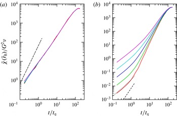
which effectively provides a Lagrangian estimate of ${\it\chi}$ based on results at a finite non-zero $\tilde{r}_{0}(T)$ approaching zero, but not exactly equal to zero. Figure 8 shows non-dimensionalized $\tilde{{\it\chi}}(\tilde{r}_{0})$ for $\tilde{r}_{0}/{\it\eta}=1/4$ to 4 at $Sc=1$ , along with the corresponding Eulerian result, for $R_{{\it\lambda}}$ ranging from $140$ to $1000$ . It can be seen that as $\tilde{r}_{0}$ becomes smaller, $\tilde{{\it\chi}}(\tilde{r}_{0})$ approaches the Eulerian result ${\it\chi}$ , with the lines in red virtually coinciding with the black dashed lines. At large times, all lines shown converge towards

which can be obtained by noting that the mean-squared relative displacement in (2.29) becomes twice the one-molecule mean-squared displacement used to obtain the scalar production term. To understand the convergence of results in the limit of $\tilde{r}_{0}\rightarrow 0$ we can consider theoretical results on $\tilde{{\it\chi}}(\tilde{r}_{0})$ at small times, If we consider pairs of very small separation only, i.e. $\tilde{r}_{0}\ll {\it\eta}$ , we can obtain the time derivative in (6.6) by differentiating (the backward version of, with a change in sign in the ballistic $t^{3}$ term) (2.17). The result, non-dimensionalized in the same manner as the production term, is

where $\langle r_{0}^{2}\rangle$ is the average over all initial separations in the bin centred on $\tilde{r}_{0}$ . This expression has a strong dependence on $\tilde{r}_{0}$ which is (to leading order) linear in time, while the last term, scaling as $t^{2}$ , is the true scalar dissipation in the limit of $\tilde{r}_{0}\rightarrow 0$ . The short dotted line of slope 2 drawn between $t/t_{{\it\eta}}=0.1$ and 1 confirms excellent agreement with the data at small times in figure 8. For a given $Sc$ and $R_{{\it\lambda}}$ , the relative magnitude of the first bracket can be controlled by choosing a sufficiently small $r_{0}$ . In figure 8 it can be seen that, at small times, $\tilde{r}_{0}/{\it\eta}=1/4$ is sufficiently small to obtain very close agreement with the Eulerian result (which becomes $(2/3Sc)(t/t_{{\it\eta}})^{2}$ ).

Figure 9.

The same as figure 8, but for $R_{{\it\lambda}}=390$ at (a) $Sc=0.01$ and (b) $Sc=100$ . In each panel the black dotted line represents (6.8) while the black dashed line represents the Saffman term in the same equation with $\tilde{r}_{0}=0$ .

As noted earlier, one advantage of the Lagrangian approach adopted here is that it is able to provide results on the statistics of the scalar field when $Sc$ is far from unity more easily than in the Eulerian frame. In figure 9 we show results for $\tilde{{\it\chi}}(\tilde{r}_{0})$ for various $\tilde{r}_{0}$ at one very low value (0.01) and one very high value (100) of $Sc$ , at the highest $R_{{\it\lambda}}$ (390) for which we have such data available. Both are clearly quite distinct from the case of $Sc=1$ at the same $R_{{\it\lambda}}$ , which is already shown in figure 8(b).

For $Sc=0.01$ , we can see that the curves for all $\tilde{r}_{0}/{\it\eta}$ almost completely overlap, since molecular diffusion effects are so strong that the effect of $\tilde{r}_{0}$ is almost negligible. The discrepancy between the DNS data lines and the Saffman limit (which has slope $2$ in this figure) is because the observation times $t$ do not satisfy the condition $t/t_{{\it\eta}}\ll Sc=0.01$ . We see though that the results are trending towards the Saffman limit with decreasing time.

A substantial contrast for $Sc=100$ is evident in figure 9(b), where the $\tilde{r}_{0}$ dependence is very strong. While the data at small times agree very well with (6.8), in this case well-sampled results for $\tilde{r}_{0}$ substantially smaller than ${\it\eta}/4$ are necessary to approximate the limiting case $\tilde{r}_{0}\rightarrow 0$ well. This is a challenging requirement, since a substantial increase in the number of pairs of small separation can be achieved only by tracking a much larger population of molecules. The need for more samples will also grow with increasing Reynolds number, such that a satisfactory convergence to $\tilde{r}_{0}\rightarrow 0$ at high $Sc$ and high $R_{{\it\lambda}}$ would be almost impossible to achieve in practice. However, $\tilde{{\it\chi}}(\tilde{r}_{0}/{\it\eta}=1/4)$ provides a better estimate for the dissipation at larger times, and particularly for the stationary state, as the dependence on $\tilde{r}_{0}$ weakens and eventually vanishes.

In (6.5) and (6.7), it has already been noted that in the large-time limit, both the production and the dissipation approach $2{\it\sigma}_{u}^{2}T_{m}/{\it\nu}$ under the normalization used above. A semi-empirical estimate of this dimensionless quantity can be made by writing it in terms of the Reynolds number and several time scales in turbulence, as

where the Eulerian large-eddy time scale $T_{E}={\it\sigma}_{u}^{2}/\langle {\it\epsilon}\rangle$ , and for $R_{{\it\lambda}}\geqslant 140$ the ratio of the Lagrangian to Eulerian time scales is $T_{L}/T_{E}=2/\tilde{C}_{0}$ , with $\tilde{C}_{0}\approx 6.5$ (Sawford et al. Reference Sawford, Yeung and Hackl2008). Thus, we have the result

where the ratio $T_{m}/T_{L}$ has (as in table 2) a very weak dependence on $Sc$ at large $R_{{\it\lambda}}$ .

Figure 10.

Evolution of normalized rates of production (a) and the quantity $\tilde{{\it\chi}}(\tilde{r}_{0}/{\it\eta}=1/4)$ (b) computed from molecular statistics for $R_{{\it\lambda}}=140$ (solid lines) and 390 (dashed lines), at $Sc=0.01$ (red), 1 (green) and 100 (blue). The Schmidt number increases from bottom to top in (a) but top to bottom in (b). For production, the lines for $Sc=1$ and $100$ are virtually indistinguishable. The horizontal black dotted lines drawn for comparison are at heights $0.041{R_{{\it\lambda}}}^{2}$ .

It is worth recapitulating that, to leading order and in the limit of vanishing backward initial separation, the rate of production of scalar fluctuations is initially independent of $Sc$ according to (6.4), whereas the rate of dissipation is initially independent of Reynolds number according to (6.8). Figure 10 shows the evolution of both production and $\tilde{{\it\chi}}(\tilde{r}_{0}/{\it\eta}=1/4)$ , our Lagrangian approximation to the scalar dissipation, as they eventually approach the same large-time limit represented by (6.10). The behaviour at small times is exactly as expected from (6.4) and (6.8). At large times, for $R_{{\it\lambda}}=140$ , both scalar production and dissipation approach the same stationary state, although the curves for $Sc=0.01$ are distinctively lower than that of $Sc\gtrsim 1$ . However, at $R_{{\it\lambda}}=390$ , we observe that all $Sc$ cases nearly overlap at large times, since for the same $Sc$ , $T_{m}/T_{L}$ is closer to unity for $R_{{\it\lambda}}=390$ compared with $R_{{\it\lambda}}=140$ . This observation that in the stationary state the scalar dissipation becomes independent of $Sc$ with increasing $R_{{\it\lambda}}$ , which in this case is derived from Lagrangian displacement statistics of molecules, is consistent with the corresponding Eulerian view of the scalar dissipation anomaly (Donzis, Sreenivasan & Yeung Reference Donzis, Sreenivasan and Yeung2005), and is evidence for so-called ‘spontaneous stochasticity’ (Bernard, Gawedzki & Kupiainen Reference Bernard, Gawedzki and Kupiainen1998; Eyink Reference Eyink2011). As a consequence, in the large-Reynolds-number limit fluid particles can be used in place of molecules to calculate scalar statistics on scales outside the dissipation subrange.

Finally, we examine the evolution of the non-dimensional scalar time scale, in the form of the ratio of the scalar field time scale $\langle {\it\phi}^{2}\rangle /\langle {\it\chi}\rangle$ to the turbulence time scale $K/\langle {\it\epsilon}\rangle$ , where $K=3/2{\it\sigma}_{u}^{2}$ is the turbulence kinetic energy. At very small times, from (2.24) we have $\langle {\it\phi}^{2}\rangle \approx {\it\sigma}_{u}^{2}t^{2}G^{2}$ , while from (6.8) in the limit $\tilde{r}_{0}\rightarrow 0$ we have $\langle {\it\chi}\rangle \approx 2/3Sc^{-1}(t^{2}/t_{{\it\eta}}^{2})G^{2}{\it\nu}$ . This readily leads to

Data for the non-dimensional scalar time scale in the large-time stationary limit in DNS have been examined by Borgas et al. (Reference Borgas, Sawford, Xu, Donzis and Yeung2004) (for $Sc\geqslant 1$ ) and Donzis et al. (Reference Donzis, Sreenivasan and Yeung2005) (for $Sc\geqslant 1/8$ ). Both present semi-empirical results, based on integration of the scalar spectrum, describing the dependence of the time scale on the Reynolds number and Schmidt number. For $Sc=1$ the result given by Borgas et al. (Reference Borgas, Sawford, Xu, Donzis and Yeung2004) is simpler (and is found to fit the data slightly better). It is of the form

where values of $a=0.41$ and $b=4.33$ represent the DNS data well. Clearly, (6.12) breaks down for $R_{{\it\lambda}}=0$ , but we are mostly interested in the large-Reynolds-number limit. For $Sc\gg 1$ both groups propose a correction logarithmic in Schmidt number, which arises from the Batchelor $k^{-1}$ spectrum (Batchelor Reference Batchelor1959), so that (6.12) becomes

where $B_{{\it\phi}}\approx 5$ (Borgas et al. Reference Borgas, Sawford, Xu, Donzis and Yeung2004; Donzis et al. Reference Donzis, Sreenivasan and Yeung2010) is the Batchelor constant. For $Sc\ll 1$ , Donzis et al. (Reference Donzis, Sreenivasan and Yeung2005) propose an inverse square-root correction, so in this case (6.12) becomes

Figure 11.

Evolution of the ratio of scalar to mechanical time scales. The dashed lines in (a) represent Eulerian data for $Sc=1/8$ (lower curve) and $Sc=1$ (upper curve). The corresponding solid lines are smoothing functions satisfying the small- and large-time limits (6.11)–(6.14). Panel (b) shows these smoothing functions (the dashed and solid curves are for $Sc=1/8$ and 1 respectively) from fits to data at $R_{{\it\lambda}}=140$ (red), 240 (blue), 390 (magenta) and 650 (cyan) (bottom to top at small times). The dashed lines in (c) show Lagrangian data (for $\tilde{r}_{0}/{\it\eta}=1/4$ ) at $R_{{\it\lambda}}=140$ for $Sc=0.01$ (black), 0.125 (blue), 1 (cyan), 8 (green), 100 (red) and 1000 (magenta) (bottom to top). The corresponding solid lines are smoothing functions interpolated to the small-time limit (6.11).

Here, we take $c=1.25$ . The data used in developing these semi-empirical relations were averaged over an extended time period of several eddy-turnover times in a stationary state, whereas the present data are time series subject to significant sampling variation, particularly at low Reynolds number. In order to smooth out these variations, we have fitted suitable functions, typically an exponential decay with a linear correction, to the data. These functions have been constrained to satisfy the small-time limit (6.11) and the stationary limits (6.12)–(6.14). Figure 11(a) shows the result of such a fit to Eulerian time series for $Sc=1/8$ and $Sc=1$ at $R_{{\it\lambda}}=140$ . Given the variation, particularly at large times, the fitted functions are good representations of the data. The sampling variation decreases, and the fits improve, with increasing Reynolds number. Figure 11(b) shows the fitted functions for $R_{{\it\lambda}}=140{-}650$ . There are two points to note. First, at small times, the time scale is directly proportional to $Sc$ even in the large-Reynolds-number limit, so molecular diffusion can never be neglected. Second, in the stationary state for fixed $Sc$ , the time scale becomes independent of $Sc$ with increasing Reynolds number. This is again a manifestation of the scalar dissipation anomaly. These findings are confirmation of the small- and large-time predictions presented above. Finally, figure 11(c) shows results as a function of $Sc$ at $R_{{\it\lambda}}=140$ . In this case we show Lagrangian results for $\tilde{r}_{0}/{\it\eta}=1/4$ , which approximate the dissipation rate and hence the scalar time scale, since our Eulerian results do not cover a wide range of $Sc$ . We see that at small times our results, shown as the dashed lines, deviate from the limit (6.11) because $\tilde{r}_{0}/{\it\eta}=1/4$ is not small enough. Nevertheless, we have again been able to use suitable functional forms, shown as the solid lines, to fit our data and interpolate to the small-time limit. In this case of fixed Reynolds number, we see that with increasing $Sc$ , the time scale in the stationary limit increases in agreement with the logarithmic dependence in (6.13). Thus, in agreement with the theory developed in Borgas et al. (Reference Borgas, Sawford, Xu, Donzis and Yeung2004) and Donzis et al. (Reference Donzis, Sreenivasan and Yeung2005), our data show that the limit ${\it\kappa}\rightarrow 0$ is singular. For $R_{{\it\lambda}}\rightarrow \infty$ at finite $Sc$ the scalar dissipation and the scalar time scale are independent of molecular diffusion. On the other hand, for $Sc\rightarrow \infty$ at finite $R_{{\it\lambda}}$ the scalar dissipation vanishes and the scalar time scale diverges.