





1 Introduction
1.1 The focusing cubic Schrödinger equation on the line
We consider the focusing cubic Schrödinger equation in one space dimension

The Cauchy problem for (1.1) is globally well-posed in
$L^2(\mathbb R)$
 , see, for example, [Reference Tsutsumi83]. The focusing cubic Schrödinger equation (1.1) is a prime example of a completely integrable nonlinear dispersive equation on the line in the sense that it admits a Lax pair formulation as well as Bäcklund transformations.
We recall that (1.1) is invariant with respect to the scaling

Moreover, (1.1) is invariant under Galilei boosts, phase shifts, and spatial translations, which means that if
$\psi (t,x)$
 is a solution to (1.1), then for any
$p, \gamma , \sigma \in \mathbb R$
 the function

is also a solution to (1.1).
Two important features of the dynamics of the focusing cubic Schrödinger equation on the line are the modified scattering behavior of dispersive solutions to (1.1) and the existence of solitary wave solutions to (1.1).
The modified scattering behavior is related to the weak dispersion in one space dimension. More specifically, solutions to the linear Schrödinger equation on the line only decay in
$L^\infty (\mathbb R)$
 at the slow rate
$t^{-\frac 12}$
 as
$t \to \infty $
 . The cubic nonlinearity is therefore long-range and the asymptotics of dispersive solutions to (1.1) are bound to feature corrections with respect to the free flow.
An example of a solitary wave solution to (1.1) is given by

The invariance of (1.1) under scaling, Galilei boosts, phase shifts, and spatial translations then generates the following 4-parameter family of solitary waves

where we use the notation

for the unique positive even ground state solution to the equation

A fundamental question concerning the family of solitary waves (1.3) is their stability under the flow of (1.1) with respect to small perturbations. Orbital stability in
$H^1(\mathbb R)$
 follows from the classical works [Reference Cazenave and Lions6, Reference Shatah and Strauss78, Reference Weinstein85, Reference Weinstein86, Reference Grillakis, Shatah and Strauss30]. Exploiting the complete integrability of (1.1), one can in fact show that orbital stability holds with respect to weaker topologies, see for instance [Reference Mizumachi and Pelinovsky67, Reference Koch and Tataru41]. The asymptotic stability of the family of solitary waves (1.3) with respect to perturbations that are small in weighted Sobolev norms was established in [Reference Cuccagna and Pelinovsky19, Reference Saalmann76, Reference Borghese, Jenkins and McLaughlin1] using complete integrability techniques. For perturbations in the energy space, asymptotic stability of (1.3) cannot hold since the family of 2-solitons constructed by the inverse scattering transform in [Reference Olmedilla71, Reference Zakharov and Shabat87] provides counter-examples, as pointed out in [Reference Martel62].
1.2 Main result
In this work we study the asymptotic stability problem for the family of solitary waves (1.3) using perturbative techniques that do not rely on the complete integrability of the focusing cubic Schrödinger equation on the line. Specifically, we combine modulation techniques with a space-time resonances approach based on the distorted Fourier transform. For technical reasons we restrict to even solutions to (1.1). Our main result establishes the asymptotic stability of the 2-parameter family of (even) solitary waves

with respect to even perturbations that are small in a weighted Sobolev norm.
A common difficulty of asymptotic stability problems for solitary wave solutions to nonlinear Schrödinger equations on the line with low power nonlinearities is the weak dispersion in one space dimension. In the case of the focusing cubic Schrödinger equation (1.1), an additional significant challenge is the slow local decay caused by the threshold resonances of the linearized operator around the solitary waves (1.5). We uncover that in the case of the focusing cubic Schrödinger equation the worst effects of the threshold resonances are suppressed by two remarkable null structures of the quadratic nonlinearities. Beyond the intrinsic interest in this problem, we also view it as a valuable and instructive step to further develop perturbative techniques to approach related asymptotic stability problems for solitary waves of (nonintegrable) Schrödinger models on the line with threshold resonances or internal modes, where much remains to be understood in the absence of favorable structures.
The following is the main result of this work.
Theorem 1.1. For any
$\omega _0 \in (0,\infty )$
 there exist constants
$0 < \varepsilon _0 \ll 1$
 ,
$0 < \delta \ll 1$
 , and
$C_0 \geq 1$
 with the following property: Let
$\gamma _0 \in \mathbb R$
 and let
$u_0 \in H^1_x(\mathbb R) \cap L^{2,1}_x(\mathbb R)$
 be even with

Then the
$H^1_x \cap L^{2,1}_x$
 –solution
$\psi (t,x)$
 to (1.1) with initial condition

exists globally in time and admits a decomposition

for some continuously differentiable paths
$(\omega , \gamma ) \colon [0,\infty ) \to (0,\infty ) \times \mathbb R$
 so that

Moreover, there exists
$\omega _\infty \in (0,\infty )$
 such that

The asymptotics of the radiation term
$u(t,x)$
 exhibit logarithmic phase corrections with respect to the free flow: there exist
$W_-,W_+ \in L^\infty (\mathbb R)$
 such that uniformly for all
$x\in \mathbb R$
 and all
$t \geq 1$
 ,

where

and

Analogous statements hold for negative times
$t \leq 0$
 .
Remark 1.2. We compare the statement of Theorem 1.1 with the asymptotic stability results obtained in [Reference Borghese, Jenkins and McLaughlin1, Reference Cuccagna and Pelinovsky19, Reference Saalmann76] using complete integrability techniques. While [Reference Borghese, Jenkins and McLaughlin1, Reference Cuccagna and Pelinovsky19, Reference Saalmann76] do not impose parity restrictions, we consider even perturbations for technical reasons explained in Remark 1.3 below. As in [Reference Borghese, Jenkins and McLaughlin1, Reference Cuccagna and Pelinovsky19, Reference Saalmann76] we prove that the radiation term decays at the rate (1.8) of linear Schrödinger waves in one space dimension, and as in [Reference Borghese, Jenkins and McLaughlin1, Reference Saalmann76] we obtain asymptotics (1.10) for the radiation term that uncover logarithmic phase corrections with respect to the corresponding free flow. We determine the scaling parameter
$\omega _\infty $
 for the final soliton, but unlike [Reference Borghese, Jenkins and McLaughlin1, Reference Cuccagna and Pelinovsky19, Reference Saalmann76] a small uncertainty regarding the phase shift parameter of the final soliton remains due to the nonintegrable decay rate (1.9). Our assumptions on the initial perturbations are slightly stronger than in [Reference Borghese, Jenkins and McLaughlin1, Reference Cuccagna and Pelinovsky19, Reference Saalmann76].
However, in contrast to [Reference Borghese, Jenkins and McLaughlin1, Reference Cuccagna and Pelinovsky19, Reference Saalmann76] the strategy of our proof combining modulation techniques and a space-time resonances approach based on the distorted Fourier transform is applicable to many other asymptotic stability problems for solitary wave solutions to nonlinear Schrödinger equations. In particular, we view the analysis in this work for the focusing cubic Schrödinger equation as a valuable and instructive step towards studying asymptotic stability problems for Schrödinger models on the line with threshold resonances or internal modes, where much remains to be understood in the absence of favorable structures.
Remark 1.3. The restriction to even perturbations in the statement of Theorem 1.1 is for the following technical reason. If we considered arbitrary perturbations, we would also have to take into account the invariance of (1.1) under Galilei boosts and under spatial translations. Correspondingly, we would have to track the evolution of two additional modulation parameters. We found that the modulation equation for the Galilei boost parameter
$p(t)$
 also exhibits a remarkable null structure, analogous to the crucial null structure in the modulation equation for the scaling parameter
$\omega (t)$
 , see Lemma 6.3 and Section 8. Thus, we could seek to extend the strategy of the proof of Theorem 1.1 to this more general setting. However, related to the fact that we do not obtain integrable decay rates in (1.9) in the statement of Theorem 1.1, we would be facing a small uncertainty in the localization of the center of the modulated solitary wave. This would lead to small additional losses in the weighted energy estimates for the renormalized quadratic nonlinearities in Section 9, and we would not be able to close the bootstrap estimates in the same manner as in Section 9. Overcoming the additional challenges caused by the uncertainty in the localization of the center of the modulated solitary wave necessitates further new techniques beyond the scope of this paper.
1.3 References
The literature on the asymptotic stability of solitary wave solutions to nonlinear Schrödinger equations and related models is vast. Recently, this topic has received significant attention especially in one space dimension, where the combination of weak dispersion, low power nonlinearities, and intriguing spectral features leads to a rich class of dynamics.
For problems in one space dimension, it has become customary to distinguish two notions of asymptotic stability, which complement each other. Local asymptotic stability refers to convergence of the perturbed solution locally in space to a final soliton, usually under weak assumptions such as small finite energy perturbations. Full (or detailed) asymptotic stability includes decay rates and asymptotics for the convergence to the final soliton at the expense of stronger assumptions on the initial perturbations such as smallness with respect to weighted Sobolev norms.
The analysis in this paper combines a circle of ideas and techniques related to modified scattering, modulation, and distorted Fourier theory. In what follows, we point the reader to the most relevant related articles, mostly focusing on problems in one space dimension. We refer to the surveys [Reference Cuccagna and Maeda13, Reference Kowalczyk, Martel and Muñoz46, Reference Schlag77, Reference Tao82] for a more exhaustive list of references, especially for results in higher space dimensions and for related models.
The modified scattering of small solutions to cubic Schrödinger equations on the line with or without potential has been studied in [Reference Hayashi and Naumkin31, Reference Lindblad and Soffer58, Reference Kato and Pusateri39, Reference Ifrim and Tataru36, Reference Germain, Pusateri and Rousset25, Reference Chen and Pusateri9, Reference Chen and Pusateri10, Reference Delort20, Reference Naumkin68, Reference Naumkin69, Reference Masaki, Murphy and Segata64, Reference Naumkin and Weder70]. For related results on the long-time behavior of small solutions to quadratic or cubic Klein-Gordon equations in one space dimension we refer to [Reference Delort21, Reference Lindblad and Soffer57, Reference Lindblad and Soffer56, Reference Hayashi and Naumkin32, Reference Hayashi and Naumkin33, Reference Hayashi and Naumkin34, Reference Delort22, Reference Stingo81, Reference Candy and Lindblad5, Reference Sterbenz80, Reference Lindblad and Soffer59, Reference Lindblad, Lührmann and Soffer54, Reference Lindblad, Lührmann and Soffer55, Reference Lindblad, Lührmann, Schlag and Soffer53, Reference Germain and Pusateri24]. Full asymptotic stability results for large solitary wave solutions to Schrödinger equations on the line have been obtained in [Reference Buslaev and Perelman2, Reference Buslaev and Sulem4, Reference Krieger and Schlag49, Reference Collot and Germain11, Reference Masaki, Murphy and Segata65], while local asymptotic stability results include [Reference Martel62, Reference Martel63, Reference Rialland74, Reference Rialland75, Reference Cuccagna and Maeda17, Reference Cuccagna and Maeda16]. For small solitary wave solutions to Schrödinger equations in one space dimension we refer to [Reference Mizumachi66, Reference Chen8] for full asymptotic stability results and to [Reference Cuccagna and Maeda12, Reference Cuccagna and Maeda14] for local asymptotic stability results. Closely related are the following full asymptotic stability results [Reference Kopylova and Komech42, Reference Kopylova and Komech43, Reference Germain and Pusateri24, Reference Lührmann and Schlag60, Reference Germain, Pusateri and Zhang26, Reference Kairzhan and Pusateri38, Reference Lührmann and Schlag61] and the following local asymptotic stability results [Reference Kowalczyk, Martel and Muñoz45, Reference Kowalczyk, Martel and Muñoz47, Reference Kowalczyk, Martel, Muñoz and Van Den Bosch48, Reference Kowalczyk and Martel44, Reference Li and Lührmann52, Reference Cuccagna and Maeda15, Reference Cuccagna, Maeda, Murgante and Scrobogna18, Reference Palacios and Pusateri72] for solitons in scalar field theories on the line.
References for the spectral and distorted Fourier theory as well as for linear dispersive estimates for scalar and matrix Schrödinger operators in one space dimension include [Reference Weder84, Reference Goldberg and Schlag29, Reference Goldberg28, Reference Chang, Gustafson, Nakanishi and Tsai7, Reference Krieger and Schlag49, Reference Li51, Reference Buslaev and Perelman2].
As pointed out at the beginning of the introduction, using complete integrability techniques the full asymptotic stability of the family of solitary wave solutions (1.3) to the focusing cubic Schrödinger equation was established in [Reference Cuccagna and Pelinovsky19, Reference Saalmann76, Reference Borghese, Jenkins and McLaughlin1].
Closely related articles. We conclude our literature overview with a brief discussion of the articles that are very closely related to our work. Co-dimensional asymptotic stability for solitary wave solutions to super-critical focusing Schrödinger equations
$i\partial _t \psi + \partial _x^2 \psi + |\psi |^{p-1} \psi = 0$
 ,
$p> 5$
 , on the line was established in [Reference Krieger and Schlag49]. Related earlier results were obtained in [Reference Buslaev and Perelman2] under tailored assumptions on the nonlinearity and the spectrum of the linearized operator. The analysis in [Reference Krieger and Schlag49] combines modulation to take into account the symmetries of the equation with a dispersive setup largely based on Strichartz estimates, which suffices for the higher power nonlinearities considered in [Reference Krieger and Schlag49]. Moreover, [Reference Krieger and Schlag49] systematically develops the spectral and distorted Fourier theory as well as linear dispersive decay estimates for matrix linearized Schrödinger operators around solitary waves with no threshold resonance (generic case). More recently, [Reference Collot and Germain11] established full asymptotic stability of solitary waves for general nonlinear Schrödinger equations
$i\partial _t \psi + \partial _x^2 \psi + F'(|\psi |^2) \psi = 0$
 allowing for cubic nonlinearities under the key assumption that the matrix linearized Schrödinger operator exhibits neither nonzero eigenvalues nor threshold resonances (generic case). To deal with modified scattering dynamics related to the long-range nature of the cubic nonlinearity, the analysis in [Reference Collot and Germain11] combines modulation with a space-time resonances approach based on the distorted Fourier transform. Previously, a similar strategy had been developed in [Reference Chen8] in the related context of proving the full asymptotic stability of small solitary wave solutions to cubic Schrödinger equations on the line with a trapping potential.
The analysis in this work further develops the framework from [Reference Collot and Germain11] to prove full asymptotic stability of solitary waves of the focusing cubic Schrödinger equation on the line, where the linearized matrix operator additionally exhibits threshold resonances (nongeneric case). We also need to set up the distorted Fourier theory for this linearized operator building on the generic case treated in [Reference Krieger and Schlag49], and we establish linear dispersive decay estimates building on results from [Reference Li51]. Moreover, we use a variable coefficient normal form reminiscent of the one employed in the proof of full asymptotic stability of the sine-Gordon kink under odd perturbations in [Reference Lührmann and Schlag60], and we benefit from insights from the study of the long-time behavior of small solutions to nonlinear Klein-Gordon equations in one space dimension in the presence of a threshold resonance in the series of articles [Reference Lindblad, Lührmann and Soffer54, Reference Lindblad, Lührmann and Soffer55, Reference Lindblad, Lührmann, Schlag and Soffer53, Reference Lührmann and Schlag60, Reference Lührmann and Schlag61].
1.4 Overview of the proof
In this subsection we provide an overview of the main ideas entering the proof of Theorem 1.1.
Linearized Operator. Writing the focusing cubic Schrödinger equation (1.1) as a system for the vector
$(\psi , \bar {\psi })$
 and linearizing around a solitary wave
$e^{i\omega t} e^{i\gamma } \phi _\omega (x)$
 for some fixed
$\omega \in (0,\infty )$
 ,
$\gamma \in \mathbb R$
 , we arrive at the nonselfadjoint matrix Schrödinger operator

This operator is closed on
$H^2_x(\mathbb R) \times H^2_x(\mathbb R)$
 and its spectrum is well-known:
$\mathcal H(\omega )$
 has essential spectrum
$(-\infty , -\omega ] \cup [\omega , \infty )$
 with no embedded eigenvalues. The only eigenvalue is
$0$
 with algebraic multiplicity equal to
$4$
 and geometric multiplicity equal to
$2$
 . Its generalized eigenfunctions are generated by the symmetries, that is, the invariance of (1.1) under phase shifts, scaling, spatial translations, and Galilei boosts. They are explicitly given by

and it holds that

The vector-valued functions
$Y_{1,\omega }, Y_{2,\omega }$
 are even, while
$Y_{3,\omega }, Y_{4,\omega }$
 are odd. Since we only study even solutions to (1.1), we consider
$\mathcal H(\omega )$
 restricted to the subspace of even functions. The eigenvalue
$0$
 then has algebraic multiplicity
$2$
 and geometric multiplicity
$1$
 . Moreover,
$\mathcal H(\omega )$
 exhibits an even threshold resonance at the edge of each part of the essential spectrum. Indeed, the functions

belong to
$L^\infty _x(\mathbb R) \times L^\infty _x(\mathbb R) \setminus L^2_x(\mathbb R) \times L^2_x(\mathbb R)$
 and satisfy

In Section 3 we recall the spectral theory for
$\mathcal H(\omega )$
 and we systematically develop the distorted Fourier theory for
$\mathcal H(\omega )$
 . We point out that the distorted Fourier theory established in [Reference Buslaev and Perelman2, Reference Krieger and Schlag49] for matrix Schrödinger operators of the form (1.12) in the generic case (no threshold resonances) does not directly apply to
$\mathcal H(\omega )$
 . Analogously to [Reference Buslaev and Perelman2, Reference Krieger and Schlag49], our construction of the distorted Fourier transform associated with
$\mathcal H(\omega )$
 is based on an explicit computation of the jump of the resolvent across the essential spectrum and on a representation of the linear evolution
$e^{it\mathcal H(\omega )}$
 in terms of a contour integral of the resolvent (analogue of Stone’s theorem in the nonselfadjoint case). In Section 4 we collect linear decay estimates for the linear evolution associated with the operator
$\mathcal H(\omega )$
 .
Spectrum of the operator
$\mathcal H(\omega )$
 in (1.12).

Modulation. Our starting point for the analysis of the asymptotic stability of the family of solitary waves (1.5) is to use standard modulation techniques to decompose the perturbed even solution
$\psi (t,x)$
 to (1.1) into a modulated solitary wave and a radiation term that is orthogonal to directions related to the invariance of (1.1) under scaling and phase shifts. Specifically, we write

for continuously differentiable paths
$\omega (t) \in (0,\infty )$
 with
$|\omega (t) - \omega _0| \lesssim \varepsilon $
 and
$\gamma (t) \in \mathbb R$
 that are uniquely determined by the orthogonality conditions

The resulting evolution equation for the radiation term
$U(t)$
 reads

It is coupled to the following system of first-order differential equations for the modulation parameters

In the preceding identities,
$\sigma _2, \sigma _3$
 are the Pauli matrices defined in (2.1),
${\mathcal Mod}$
 denotes relatively harmless terms that are a consequence of the time-dependence of the modulation parameters, and the quadratic and cubic nonlinearities on the right-hand sides of (1.15) and (1.16) are given by

Moreover, the matrix
$\mathbb {M}$
 on the left-hand side of (1.16) is given by

which is clearly invertible for sufficiently small perturbations
$U(t)$
 .
Schematic Setup and Strategy. Now our primary task is to simultaneously establish decay and asymptotics for the radiation term
$U(t)$
 and to prove convergence of the modulation parameter
$\omega (t)$
 to an asymptotic value
$\omega _\infty \in (0,\infty ) $
 as
$t\to \infty $
 , in other words to establish sufficiently fast decay of
$\omega (t) - \omega _\infty $
 to zero. In view of the weak dispersion in one space dimension in conjunction with the low power nonlinearities on the right-hand sides of (1.15) and (1.16), this is a formidable challenge that gets compounded by the subtle, but severe effects of the threshold resonances on the dynamics.
In order to prove decay for the radiation term by perturbative means, we naturally want to invoke dispersive estimates for the linear evolution
$i\partial _t U - \mathcal H(\omega ) U = 0$
 associated with (1.15). However, the modulation parameter
$\omega = \omega (t)$
 is time-dependent. We therefore need to pass to a time-independent reference operator
$\mathcal H({\underline {\omega }})$
 on the left-hand side of (1.15) for a suitably chosen fixed scaling parameter
${\underline {\omega }}$
 and then treat the difference perturbatively. Heuristically, we take
${\underline {\omega }}$
 to be the asymptotic limit of
$\omega (t)$
 as
$t \to \infty $
 . The proof of Theorem 1.1 proceeds via an elaborate bootstrap argument, so that on a given finite time interval
$[0,T]$
 we actually chooseFootnote
1
${\underline {\omega }} = \omega (T)$
 to be the final value of the continuously differentiable path
$\omega (t)$
 on that time interval. As part of our bootstrap argument we seek to show the decay estimate

where
$0 < \delta \ll 1$
 is a small absolute constant. Later, we will then extract the final value
$\omega _\infty $
 of the path
$\omega (t)$
 as
$t \to \infty $
 from (1.18) with
$T = T_n$
 for an increasing sequence of times
$T_n \nearrow \infty $
 . The decay rate (1.18) turns out to be just about enough to treat perturbatively the error terms that arise from passing to a time-independent reference operator. We point out that since
$\omega (t)-{\underline {\omega }} = -\int _t^T \dot {\omega }(s) \, \mathrm {d} s$
 by the fundamental theorem of calculus, an almost twice integrable in time decay rate
$s^{-2+\delta }$
 for
$\dot {\omega }(s)$
 as
$s \to \infty $
 would be necessary to crudely infer the decay estimate (1.18).
For the discussion of the main aspects of the nonlinear analysis, in what follows we only consider schematic versions of (1.15) and (1.16) that retain the most relevant terms. Specifically, in the evolution equation (1.15) for the radiation term, we disregard milder modulation terms and we pass to the reference operator
$\mathcal H({\underline {\omega }})$
 , which produces the delicate difference term
$(\omega - {\underline {\omega }}) \sigma _3 U$
 on the right-hand side. Moreover, in the quadratic nonlinearity we replace
$\phi _\omega (x)$
 by
$\phi _{\underline {\omega }}(x)$
 and ignore the resulting milder error terms. In the modulation equations (1.16), we focus on the equation for
$\dot {\omega }$
 . To unveil its leading order structure, we only keep the quadratic nonlinearity on the right-hand side and we again replace the time-dependent parameter
$\omega $
 by
${\underline {\omega }}$
 , disregarding the resulting milder error terms. Then we are facing the following schematic evolution equation for the radiation term

coupled to a differential equation for the modulation parameter
$\omega (t)$
 of the schematic form

Our overall strategy is to take a space-time resonances approach based on the distorted Fourier transform associated with the reference operator
$\mathcal H({\underline {\omega }})$
 to infer decay and asymptotics for
$U(t)$
 , while we exploit the oscillations in the equation for
$\dot {\omega }$
 to arrive at the decay estimate (1.18) for
$\omega (t) - {\underline {\omega }}$
 . As we explain next, in comparison with the generic case (no threshold resonances) considered in [Reference Collot and Germain11], this strategy is significantly compounded by the slow local decay of the radiation term caused by the threshold resonances of the linearized operator
$\mathcal H({\underline {\omega }})$
 .
Main Enemy: Slow Local Decay. Since the quadratic nonlinearity defined in (1.17) is spatially localized due to the rapid decay of the coefficient
$\phi _{\underline {\omega }}(x)$
 , the leading order behavior of
$\mathcal Q_{\underline {\omega }}(U(t))$
 is entirely governed by the local decay of the radiation term
$U(t)$
 . In view of (1.20), the same observation holds for the leading order behavior of
$\dot {\omega }(t)$
 .
In the absence of threshold resonances (generic case), the Schrödinger waves enjoy improved local decay, which simplifies the treatment of the terms
$(\omega -{\underline {\omega }}) \sigma _3 U$
 and
$\mathcal Q_{\underline {\omega }}(U)$
 on the right-hand side of (1.19) and the derivation of sufficient decay for
$\omega (t) - {\underline {\omega }}$
 . However, in our setting the threshold resonances of
$\mathcal H({\underline {\omega }})$
 lead to slow local decay. In fact, [Reference Li51, Theorem 1.1] by the first author quantifies how the slow local decay can be pinned down exactly to the contributions of the threshold resonances, while the bulk of the Schrödinger waves still enjoy improved local decay. Specifically, for the linear evolution of a (vector-valued) Schwartz function
$F$
 we have for all
$t \geq 1$
 that

where
$\underline {P_{\mathrm {e}}}$
 denotes the Riesz projection to the essential spectrum relative to
$\mathcal H({\underline {\omega }})$
 ,
$\Phi _{\pm ,{\underline {\omega }}}(x)$
 are the threshold resonances defined in (1.13), and
$c_{\pm , {\underline {\omega }}}(F)$
 should be thought of as projections of
$F$
 onto these

Thus, the leading order behavior of
$\mathcal Q_{\underline {\omega }}(U(t))$
 can be thought of as a linear combination of slowly decaying quadratic source terms of the schematic form

see the expansion (5.51) for the precise expression. These source terms create resonances both in the evolution equation (1.19) for the radiation term and in the differential equation (1.20) for
$\dot {\omega }$
 . For more detailed explanations we refer to the discussions after (5.53), respectively after (8.14). In particular, the slow
$t^{-1}$
 decay of the schematic source terms (1.21) is far away from the twice integrability in time of
$\dot {\omega }(t)$
 pointed out earlier, which would be necessary to crudely infer the decay estimate (1.18).
Null Structures. It turns out that we do not have to address the worst effects of the resonant quadratic source terms (1.21) in our analysis thanks to two remarkable null structures in the quadratic nonlinearities of the evolution equation for the radiation term as well as of the modulation equations. These null structures appear to be closely related to the completely integrable structure of the equation, but we do not have a rigorous proof for this connection.
We refer to Lemma 5.4 and the discussion in Subsection 5.4 for a quadratic null structure in the evolution equation for the radiation term. It was already observed by the first author in [Reference Li51, Lemma 1.6] and it is reminiscent of a similar null structure for perturbations of the sine-Gordon kink, see [Reference Lührmann and Schlag60, Reference Lindblad, Lührmann, Schlag and Soffer53]. Using a variable coefficient normal form inspired by [Reference Lindblad, Lührmann and Soffer55, Reference Lührmann and Schlag60], we can then recast the quadratic nonlinearity
$\mathcal Q_{\underline {\omega }}(U)$
 on the right-hand side of (1.19) into a spatially localized cubic term, which is slightly better behaved than the constant coefficient cubic term
$\mathcal C(U)$
 .
For the details of the null structure in the modulation equations we refer to Lemma 6.3 and the discussion in Section 8, specifically the treatment of the term
$I(s)$
 in (8.12). Thanks to this remarkable null structure, in the proof of the decay estimate (1.18) we can integrate by parts in the time integral of the leading order quadratic contribution

which effectively turns it into the contribution of a cubic term

We show that the latter does not exhibit any time resonances, whence we can integrate by parts in time once more and turn it into the time integral of a quartic term, which enjoys the desired crude twice integrability to conclude (1.18).
Modified Scattering Analysis. Finally, we discuss the analysis of the modified scattering behavior of the radiation term. As explained above, we can use a variable coefficient normal form to recast the quadratic nonlinearity
$\mathcal Q_{\underline {\omega }}(U)$
 on the right-hand side of (1.19) into a better behaved spatially localized cubic term. Moreover, thanks to the sufficiently fast decay (1.18) of
$\omega (t) - {\underline {\omega }}$
 , we can use an integrating factor argument inspired by [Reference Collot and Germain11, Proposition 9.5] to effectively remove the term
$(\omega -{\underline {\omega }}) \sigma _3 U$
 from (1.19), see (5.45) and (5.46). Then we are essentially reduced to studying the asymptotic behavior of small solutions to the cubic matrix Schrödinger equation

In analogy to the study of the long-time dynamics of small solutions to the scalar cubic Schrödinger equation with (or without) potential in one space dimension

we expect logarithmic phase corrections with respect to the free flow. As in the generic case considered in [Reference Collot and Germain11], we proceed in the spirit of the space-time resonances method for the scalar equation (1.23), see [Reference Kato and Pusateri39, Reference Germain, Pusateri and Rousset25, Reference Chen and Pusateri9, Reference Chen and Pusateri10], and we introduce the profile of the radiation term
$U(t)$
 relative to the reference operator
$\mathcal H({\underline {\omega }})$
 by filtering out the linear evolution

where we recall that
$\underline {P_{\mathrm {e}}}$
 denotes the projection to the essential spectrum for
$\mathcal H({\underline {\omega }})$
 .
Then the idea is to consider the evolution equation for the (vector-valued) distorted Fourier transform relative to
$\mathcal H({\underline {\omega }})$
 of the profile
$\widetilde {\mathcal F}_{\underline {\omega }}[F_{\underline {\omega }}(t)](\xi ) =: ( {{\tilde {f}}_{+,{\underline {\omega }}}}(t,\xi ), {{\tilde {f}}_{-,{\underline {\omega }}}}(t,\xi ) )$
 , which reads

We uncover the fine structure of the contributions of the cubic terms on the right-hand side of (1.25) by inserting the representation formula (5.35) for the radiation term in terms of the distorted Fourier transform of its profile. Analyzing the interactions of the corresponding distorted Fourier basis elements (cubic spectral distributions), we arrive at the decomposition

The three terms on the right-hand side of (1.26) are trilinear expressions in terms of the components of the distorted Fourier transform of the profile involving a Dirac kernel, a Hilbert-type kernel, and a regular kernel, respectively. See Section 6.1 for the details.
In view of the linear dispersive decay estimate from Lemma 4.1, in order to recover the linear decay rate
$t^{-\frac 12}$
 for the radiation term, it suffices to establish slowly growing weighted energy estimates

and uniform-in-time pointwise bounds

Thanks to a simple relation between the two components
${{\tilde {f}}_{+,{\underline {\omega }}}}(t,\xi )$
 and
${{\tilde {f}}_{-,{\underline {\omega }}}}(t,\xi )$
 , see Lemma 3.14, it in fact suffices to derive the bounds (1.27), (1.28) for the component
${{\tilde {f}}_{+,{\underline {\omega }}}}(t,\xi )$
 .
In Section 9 we establish the weighted energy estimates (1.27), where
$0 < \delta \ll 1$
 is the same small absolute constant as in (1.18). In Section 10 we infer the pointwise bounds (1.28) for the distorted Fourier transform of the profile via an ODE argument, in the course of which we capture the logarithmic phase corrections in the asymptotics of the radiation term. More specifically, we carry out a stationary phase analysis of the contributions of the cubic terms in (1.25), where we rely on their fine structure determined in (1.26). We find that the evolution equation for
$\tilde {f}_{+,{\underline {\omega }}}(t,\xi )$
 is effectively given by

where the leading order term stems from the cubic interactions with a Dirac kernel, and where the remainder term
$r(t,\xi )$
 enjoys faster decay. Using a standard integrating factor argument, we can then deduce the pointwise bounds (1.28).
Further Comments. We conclude the discussion of the main ideas of the proof of Theorem 1.1 with several more technical comments.
-
(i) Owing to the quadratic null structures uncovered in Lemma 5.4 and Lemma 6.3, the quadratic nonlinearity affects neither the asymptotics of the radiation term nor the asymptotic behavior of the modulation parameters. In the absence of favorable structures for related models with threshold resonances, this is a regime where much remains to be understood.
-
(ii) In contrast to the generic case treated in [Reference Collot and Germain11], we do not obtain integrable decay rates for $\omega (t)-\omega (T)$
 and for
$\dot {\gamma }(t)-\omega (t)$
. As a consequence, we have to handle a slight uncertainty in the phase shift in the proof of Theorem 1.1 and we do not extract the phase shift parameter for the final soliton. It is an interesting question how one could possibly further enhance the analysis in this paper to deduce integrable decay rates.
-
(iii) Interestingly, in the derivation of the differential equation to extract the asymptotics of the distorted Fourier transform of the profile in Lemma 10.4, the (critically decaying) cubic interactions with a Hilbert-type kernel do not contribute due to the vanishing property (6.10), see the proof of (10.23).
-
(iv) The null structure in the modulation equations discussed above is reminiscent of a similar favorable structure exploited in the modulation equations in [Reference Krieger and Schlag50, Lemma 5.12] in the context of constructing blow-up solutions to the critical focusing nonlinear Schrödinger equation on the line. The authors are grateful to Joachim Krieger for pointing out this connection.
-
(v) The tensorized product structure of the distorted Fourier basis elements is convenient in our analysis, see for instance Lemma 3.16 and the study of the fine structure of the cubic spectral distributions in Subsection 6.1.
-
(vi) We exploit the simple relationship (5.47) between the two components ${{\tilde {f}}_{+,{\underline {\omega }}}}(t,\xi )$
and
${{\tilde {f}}_{-,{\underline {\omega }}}}(t,\xi )$
of the distorted Fourier transform of the profile in the nonlinear analysis. It should be compared with the corresponding relation in the generic case, see, for example, [Reference Collot and Germain11, Lemma 5.12]. -
(vii) In the derivation of the slowly growing weighted energy estimates for the profile in Proposition 9.4, the dual local smoothing estimates for the Schrödinger evolution from Lemma 4.4 play a key role in handling all contributions of spatially localized nonlinearities with cubic-type time decay. This idea was first used in [Reference Chen and Pusateri10]. See also [Reference Lindblad, Lührmann and Soffer54, Reference Lindblad, Lührmann and Soffer55, Reference Lührmann and Schlag60] for a related approach.
-
(viii) We made use of the Wolfram Mathematica software system in the computation of the resolvent kernel in Subsection 3.2 as well as in the computation of the quadratic null structures in Lemma 5.4 and in Lemma 6.3.


2 Preliminaries
Notation and conventions. Throughout this paper implicit constants in estimates may depend on the initial scaling parameter
$\omega _0 \in (0,\infty )$
 fixed in the statement of Theorem 1.1. We denote by
$C> 0$
 an absolute constant whose value may change from line to line. For nonnegative
$X, Y$
 we use the notation
$X \lesssim Y$
 if
$X \leq C Y$
 and we write
$X \ll Y$
 to indicate that the implicit constant should be regarded as small. Moreover, we adopt the Japanese bracket notation

We use the standard notation for the Lebesgue spaces
$L^p$
 and for the Sobolev spaces
$H^k$
 ,
$W^{k,p}$
 . The space
$L^{2,1}$
 is defined by the weighted norm
$\|f\|_{L^{2,1}} := \|\langle x\rangle f\|_{L^2}$
 .
Pauli matrices. We recall the standard definitions of the Pauli matrices

Inner products. We define the
$L^2$
 -inner product of two scalar-valued functions
$f, g \colon \mathbb R \to \mathbb C$
 by

and the
$L^2$
 -inner product of two vector-valued functions
$U, V \colon \mathbb R \to \mathbb C^2$
 by

Fourier transform. Our conventions for the (flat) Fourier transform of a function
$f \in \mathcal S(\mathbb R)$
 are

Then the convolution laws for
$g,h \in \mathcal S(\mathbb R)$
 read

We recall that in the sense of tempered distributions


While (2.4) is standard, we refer to [Reference Lührmann and Schlag60, Lemma 5.6] for a proof of (2.5).
$\mathcal J$
 -invariance. Following the terminology in [Reference Krieger and Schlag49], we say that a vector
$U \in \mathbb C^2$
 is
$\mathcal J$
 -invariant if

The inner product (2.3) of two
$\mathcal J$
 -invariant vectors is real-valued. The
$\mathcal J$
 -invariance of the evolution equation (5.4) for the vectorial perturbation will allow us to go back from the system to the scalar cubic Schrödinger equation (1.1).
3 Spectral theory and distorted Fourier transform
Linearizing the focusing cubic Schrödinger equation (1.1) around the solitary wave solutions (1.3) leads to the following nonselfadjoint matrix Schrödinger operator

After recalling its well-known spectrum, the main purpose of this section is to systematically develop the distorted Fourier theory for
$\mathcal H(\omega )$
 .
We note that for matrix Schrödinger operators of the form (3.1) in the generic case (no threshold resonances) the distorted Fourier theory was established in [Reference Krieger and Schlag49, Reference Buslaev and Perelman2], but the results from [Reference Krieger and Schlag49, Reference Buslaev and Perelman2] do not directly apply to
$\mathcal H(\omega )$
 . Proceeding similarly to [Reference Krieger and Schlag49], we first determine the kernel of the resolvent of
$\mathcal H(\omega )$
 , which yields an explicit formula for the jump of the resolvent across the essential spectrum. Inserting the latter into a representation of the linear evolution
$e^{it\mathcal H(\omega )}$
 in terms of a contour integral of the resolvent (analogue of Stone’s theorem in the nonselfadjoint case) then naturally leads to the definition of the distorted Fourier transform associated with
$\mathcal H(\omega )$
 .
Throughout this section the following identities for the operator
$\mathcal H(\omega )$
 will be used. We have the symmetry relations

where
$\sigma _1,\sigma _2,\sigma _3$
 are the Pauli matrices defined in (2.1) and where
$\mathcal H(\omega )^\ast $
 denotes the adjoint of
$\mathcal H(\omega )$
 with respect to the inner product (2.3). Moreover, we point out a scaling relation specific to the cubic Schrödinger equation. If a function
$G(x) = (g_1(x),g_2(x))^\top $
 solves the equation

for some
$\lambda \in \mathbb C$
 , then the function
$G(\sqrt {\omega }x)=(g_1(\sqrt {\omega }x,g_2(\sqrt {\omega }x))^\top $
 solves the equation

3.1 Spectrum of linearized operator
The spectrum of the matrix Schrödinger operator
$\mathcal H(\omega )$
 is well-known. A full description is provided in the next proposition.
Proposition 3.1. Fix
$\omega \in (0,\infty )$
 . Then the following holds for the operator
$\mathcal H(\omega )$
 defined in (3.1) on
$L^2(\mathbb R) \times L^2(\mathbb R)$
 with domain
$H^2(\mathbb R) \times H^2(\mathbb R)$
 :
-
1. Discrete spectrum: $0$
is the only eigenvalue with algebraic multiplicity equal to 4 and geometric multiplicity equal to 2. -
2. Generalized nullspace: $\mathcal N_{\mathrm {g}}(\mathcal H(\omega )) = \ker (\mathcal H(\omega )^2)$
is spanned by the generalized eigenfunctions (3.5) $$ \begin{align} Y_{1,\omega} := \begin{bmatrix} i\phi_\omega \\ -i\phi_\omega \end{bmatrix}, \quad Y_{2,\omega} := \begin{bmatrix} \partial_\omega \phi_\omega \\ \partial_\omega \phi_\omega \end{bmatrix}, \quad Y_{3,\omega} := \begin{bmatrix} \partial_x \phi_\omega \\ \partial_x \phi_\omega \end{bmatrix}, \quad Y_{4,\omega} := \begin{bmatrix} ix\phi_\omega \\ -ix\phi_\omega \end{bmatrix}, \end{align} $$
which satisfy
(3.6) $$ \begin{align} \mathcal H(\omega) Y_{1,\omega} = 0,\quad \mathcal H(\omega) Y_{2,\omega} = i Y_{1,\omega}, \quad \mathcal H(\omega) {Y_{3,\omega}} = 0, \quad \mathcal H(\omega) Y_{4,\omega} = -2i Y_{3,\omega}. \end{align} $$
Moreover, we have $\mathcal N_{\mathrm {g}}(\mathcal H(\omega )^*) = \ker ((\mathcal H(\omega )^*)^2)= \mathrm {span}(\sigma _{2}Y_{k,\omega }:1\leq k\leq 4)$
, and the vectors
$Y_{k,\omega }$
and
$\sigma _2 Y_{k,\omega }$
,
$1 \leq k \leq 4$
, are
$\mathcal J$
-invariant. The functions
$Y_{1,\omega }$
,
$Y_{2,\omega }$
are even, while the functions
$Y_{3,\omega }$
,
$Y_{4,\omega }$
are odd. -
3. The essential spectrum of $\mathcal H(\omega )$
is
$(-\infty ,-\omega ] \cup [\omega ,\infty )$
and there are no embedded eigenvalues. -
4. Threshold resonances: The even vector-valued functions
(3.7) $$ \begin{align} \Phi_{+,\omega}(x) := \begin{bmatrix} \tanh^2(\sqrt{\omega}x) \\ -\operatorname{\mathrm{sech}}^2(\sqrt{\omega}x) \end{bmatrix}, \quad \Phi_{-,\omega}(x) := \sigma_1 \Phi_{+,\omega}(x) = \begin{bmatrix} -\operatorname{\mathrm{sech}}^2(\sqrt{\omega}x) \\ \tanh^2(\sqrt{\omega}x) \end{bmatrix} \end{align} $$belong to $L^\infty (\mathbb R) \times L^\infty (\mathbb R) \setminus L^2(\mathbb R) \times L^2(\mathbb R)$
and satisfy (3.8) $$ \begin{align} \mathcal H(\omega) \Phi_{+,\omega} = \omega \Phi_{+,\omega}, \quad \mathcal H(\omega) \Phi_{-,\omega} = -\omega \Phi_{-,\omega}. \end{align} $$


Remark 3.2. In the proof of Theorem 1.1 we only consider even solutions to the focusing cubic Schrödinger equation. For the restriction of
$\mathcal H(\omega )$
 to the subspace of even functions in
$H^2(\mathbb R) \times H^2(\mathbb R)$
 the eigenvalue
$0$
 has algebraic multiplicity
$2$
 and geometric multiplicity
$1$
 .
Proof of Proposition 3.1
For (2), the full description of the generalized nullspace can be found in, for example, [Reference Buslaev and Perelman3, Proposition 1.2.2.] and [Reference Weinstein85, Appendix B], and the statement for the generalized nullspace for the adjoint
$\mathcal H^*$
 follows from the symmetry relations (3.2) and (3.5). Note that a vector
$Y$
 is
$\mathcal J$
 -invariant if and only if
$\sigma _2 Y$
 is
$\mathcal J$
 -invariant. This does not necessarily hold true for
$\sigma _3 Y$
 . Furthermore, the asserted geometric and algebraic multiplicity of the zero eigenvalue in item (1) is obvious from (3.6). To show that zero is the only eigenvalue, we note that since by direct computation

the statement from [Reference Buslaev and Perelman3, Proposition 1.2.2.] implies that
$\mathrm {spec}(\mathcal H) \subset \mathbb R$
 , and by [Reference Pelinovsky, Kivshar and Afanasjev73, page 130] there are no nonzero real eigenvalues (internal modes) for
$\mathcal H$
 . For (3), the statement about the essential spectrum follows from Weyl’s criterion (see, e.g., [Reference Hundertmark and Lee35]), and the absence of embedded eigenvalues was proven in [Reference Krieger and Schlag49, Proposition 9.2]. Lastly, for (4), the formulas for
$\Phi _{\pm ,\omega }(x)$
 are obtained from [Reference Chang, Gustafson, Nakanishi and Tsai7, (3.54)] using the conjugation identity (3.12) and the rescaling identity (3.4).
3.2 Resolvent kernel
The goal of this subsection is to derive an explicit formula for the kernel of the resolvent of the operator
$\mathcal H(\omega )$
 when
$\omega = 1$
 . Afterwards, we deduce the corresponding formulas for the resolvent of
$\mathcal H(\omega )$
 for arbitrary
$\omega> 0$
 .
Adopting the same notation as in [Reference Chang, Gustafson, Nakanishi and Tsai7], we define the scalar Schrödinger operators

Then the following factorization identities hold

By [Reference Chang, Gustafson, Nakanishi and Tsai7, (3.24)], we have

and we infer from (3.9) that

Next, we introduce the matrix operators

where

The identity (3.10) implies that

Recall that the operators
$\mathcal L_0$
 and
$\mathcal L_1$
 are related to the operators
$\mathcal H_0 = \mathcal H_0(1)$
 and
$\mathcal H_1 = \mathcal H(1)$
 respectively by the conjugation identities

Upon defining

we deduce from (3.11) and (3.12) the identity

Then, using the self-adjointness of
$\mathcal H_0$
 and the symmetry relations (3.2), we infer the adjoint identity

The identity (3.14) is our starting point for the derivation of the kernel of the resolvent of
$\mathcal H_1$
 . We begin by computing a fundamental set of solutions to the equation
$\mathcal H_1 \mathbf {f} = z\mathbf {f}$
 , where
$z \in \mathbb C_+$
 is close to the positive part
$[1,\infty )$
 of the essential spectrum.
Lemma 3.3. Let
$z = \xi ^2 + 1 + i \varepsilon $
 with
$\xi \in \mathbb R$
 and
$\varepsilon>0$
 , and let
$x \in \mathbb R$
 . Denote by
$\sqrt {\cdot }$
 a branch of the square root that is analytic on
$\mathbb C \backslash [0,\infty )$
 and such that
$\sqrt {-1} = i$
 . Define the functions


Then
$\{ \mathbf {f}_1(\cdot ,z), \mathbf {f}_3(\cdot ,z), \mathbf {g}_2(\cdot ,z), {\mathbf {g}_4(\cdot ,z)} \}$
 form a fundamental set of solutions to
$(\mathcal H_1 - z)\mathbf {f} = 0$
 . Moreover, they satisfy the asymptotics

and their WronskiansFootnote 2 are given by


Proof. From the definition of
$\widetilde {\mathcal D}$
 in (3.13) we obtain that

where

For any function
$h(z)$
 , we have by direct computation

In addition, it holds that

It is straightforward to check that the following vector-valued functions

form a fundamental set of solutions to
$\mathcal H_0 \mathbf {f} = z\mathbf {f}$
 . Hence, in view of the above identities and (3.14), we can build four linearly independent solutions to
$\mathcal H_1 \mathbf {f} = z\mathbf {f}$
 as follows,

Dividing by the factor
$z$
 (or by
$-z$
 ) gives the expressions (3.15)–(3.18). By our choice of branch for the square root, we note that
$\mathrm {Re} (\sqrt {1-z}) < 0$
 as well as
$\mathrm {Re} ( \sqrt {1+z} )> 0$
 for
$z = \xi ^2 + 1 + i\varepsilon $
 with
$\xi \in \mathbb R$
 and
$\varepsilon> 0$
 . Thus, the asserted limits (3.19) follow from the expressions (3.15)–(3.18). The formulas (3.20), (3.21), (3.22) for the Wronskians follow by direct computation.
Remark 3.4. The explicit formulas for the Jost functions
$\mathbf {f}_1$
 and
$\mathbf {g}_4$
 for
$z=\xi ^2+1+i0$
 are already contained in [Reference Kaup40]. An analogous derivation of these formulas using the identity (3.14) as in the proof of the preceding Lemma 3.3 was recently given in [Reference Cuccagna and Maeda17, Section 10].
Next, we define for
$x\in \mathbb R$
 and
$z = \xi ^2 + 1 + i \varepsilon $
 with
$\xi \in \mathbb R$
 and
$\varepsilon> 0$
 , the
$2 \times 2$
 matrix-valued functions


where the functions
$\mathbf {f}_1$
 ,
$\mathbf {f}_3$
 ,
$\mathbf {g}_2$
 , and
$\mathbf {g}_4$
 on the right-hand sides are defined as in the statement of the preceding Lemma 3.3. Proceeding as in the proof of [Reference Krieger and Schlag49, Lemma 6.5], we now express the kernel of the resolvent of
$\mathcal H_1$
 in terms of the matrices
$\mathbb F$
 ,
$\mathbb G$
 , and
$\mathbb D$
 defined above.
Lemma 3.5. Let
$z = \xi ^2+1+i\varepsilon $
 with
$\xi \in \mathbb R$
 and
$\varepsilon>0$
 . We have

In particular, for
$x \geq y$
 it holds that

while for
$x \leq y$
 it holds that

Proof. We want to find the Green’s function for the system of equations

where
$\mathbf {h} \in L^2(\mathbb R) \times L^2(\mathbb R)$
 is given. In view of the asymptotics (3.19), an
$L^2(\mathbb R)$
 -integrable solution to (3.29) takes the form

where the matrices
$\mathbb M_1$
 and
$\mathbb M_2$
 are required to satisfy the compatibility conditions

This system of equations can be written in matrix form as

Using that
$\mathbb D = \mathbb D^\top $
 and applying [Reference Krieger and Schlag49, (5.22)], we have

whence

Finally, we obtain the expressions (3.27)–(3.28) for the resolvent kernels by direct computation from (3.31), (3.30) and from the explicit expressions (3.15)–(3.18) as well as (3.20)–(3.22).
Next, we compute the formula for the jump of the resolvent across the positive part
$[1,\infty )$
 of the essential spectrum.
Lemma 3.6. For
$x, \xi \in \mathbb R$
 set

and

Then for any
$\xi>0$
 ,

Proof. Let
$z_\varepsilon := \xi ^2 + 1 + i \varepsilon $
 with
$\xi> 0$
 and
$\varepsilon>0$
 . Note that

We first consider the case
$x \geq y$
 . From (3.27), we have

Thus, we also obtain that

Then using that
$(\xi ^2+1)^2 = (\xi -i)^2(\xi +i)^2$
 , we find

This proves (3.34) for
$x \geq y$
 . For the case
$x \leq y$
 we repeat the preceding computations using (3.28), which gives the same formula.
The functions
$\mathbf {F}(x,\xi )$
 and
$\mathbf {G}(x,\xi )$
 form a pair of bounded solutions to the equation
$\mathcal H_1\mathbf { f}=(\xi ^2+1)\mathbf {f}$
 . The identity (3.34) expresses a product-type formula for the jump of the resolvent across
$[1,\infty )$
 . The scaling relations (3.3)–(3.4) then imply that for arbitrary
$\omega>0$
 , the functions
$\mathbf { F}(\sqrt {\omega }x, \frac {\xi }{\sqrt {\omega }})$
 ,
$\mathbf {G}(\sqrt {\omega }x, \frac {\xi }{\sqrt {\omega }})$
 are a pair of bounded solutions to the equation
$\mathcal H(\omega )\mathbf {f} = (\xi ^2+\omega )\mathbf {f}$
 . The next corollary describes the jump of the resolvent for arbitrary
$\omega> 0$
 in terms of these rescaled functions. The proof proceeds along the lines of the preceding Lemma 3.6.
Corollary 3.7. Fix
$\omega \in (0,\infty )$
 . For
$x, \xi \in \mathbb R$
 set

Then for any
$\xi>0$
 ,

We denote by
$P_{\mathrm {d}}$
 the Riesz projection onto the discrete spectrum of
$\mathcal H(\omega )$
 defined as

where
$\gamma $
 is a simple closed curve around the origin that lies within the resolvent set of
$\mathcal H(\omega )$
 . Then we define the projection onto the essential spectrum by

We refer the reader to [Reference Krieger and Schlag49, Remark 9.5] for a proof of the fact that the Riesz projections
$P_{\mathrm {d}}$
 and
$P_{\mathrm {e}}$
 preserve the space of
$\mathcal J$
 -invariant functions on
$L^2(\mathbb R) \times L^2(\mathbb R)$
 . The next lemma provides an explicit decomposition of
$L^2(\mathbb R) \times L^2(\mathbb R)$
 into the spectral subspaces associated with the essential spectrum and with the discrete spectrum of
$\mathcal H(\omega )$
 .
Lemma 3.8. There is the decomposition

where the individual summands are linearly independent, but not necessarily orthogonal. The decomposition (3.38) is invariant under the flow of
$\mathcal H(\omega )$
 , and the projection
$P_{\mathrm {e}}$
 is the projection onto the orthogonal complement in (3.38). Explicitly, for
$U \in L^2(\mathbb R) \times L^2(\mathbb R)$
 it holds that

with

By direct computation, we have

For even
$U \in L^2(\mathbb R) \times L^2(\mathbb R)$
 it follows that

The projection
$P_{\mathrm {e}}$
 is bounded as an operator
$H^1(\mathbb R) \to H^1(\mathbb R)$
 ,
$L^{2,1}(\mathbb R) \to L^{2,1}(\mathbb R)$
 , and as an operator
$L^p(\mathbb R) \to L^p(\mathbb R)$
 for any
$1 \leq p \leq \infty $
 .
Proof. We only prove (3.39) and (3.41), and refer to the proof of Lemma 9.4 in [Reference Krieger and Schlag49] for the first part of the statement of the lemma. The identity (3.39) follows from (3.38) and the fact that
$\mathcal N_g(\mathcal H(\omega ))$
 is spanned by
$Y_{j,\omega }$
 ,
$1 \leq j \leq 4$
 , see Proposition 3.1. Since
$P_{\mathrm {e}} U$
 is orthogonal to
$\mathcal N_g(\mathcal H(\omega )^\ast )$
 and since
$\mathcal N_g(\mathcal H(\omega )^\ast )$
 is spanned by
$\sigma _2 Y_{k,\omega }$
 ,
$1 \leq k \leq 4$
 , see Proposition 3.1, we obtain from (3.39) for
$1 \leq k \leq 4$
 that

The asserted formulas for
$d_{j,\omega }$
 now follow from the facts that
$Y_{1,\omega }$
 ,
$Y_{2,\omega }$
 are even, while
$Y_{3,\omega }, Y_{4,\omega }$
 are odd, and that
$\langle Y_{j,\omega }, \sigma _2 Y_{j,\omega } \rangle = 0$
 for
$1 \leq j \leq 4$
 . The identity (3.41) for even
$U \in L^2(\mathbb R) \times L^2(\mathbb R)$
 follows immediately from (3.39) because
$Y_{3,\omega }, Y_{4,\omega }$
 are odd. Finally, the asserted boundedness properties of the projection
$P_{\mathrm {e}}$
 are a consequence of (3.39) and the fact that the generalized eigenfunctions
$Y_{j,\omega }$
 ,
$1 \leq j \leq 4$
 , are Schwartz functions.
Finally, we recall from Lemma 12 and Remark 1 in [Reference Erdoğan and Schlag23] a representation of the (nonunitary) flow
$e^{it\mathcal H(\omega )}$
 in terms of the jump of the resolvent across the essential spectrum. The statement is analogous to Stone’s formula for self-adjoint Schrödinger operators, where it is a consequence of the spectral theorem.
Proposition 3.9. There is the representation formula

3.3 Distorted Fourier theory
Now we are in a position to introduce the distorted Fourier transform relative to
$\mathcal H(\omega )$
 . We essentially read off its definition from the representation formula (3.42) for the flow
$e^{it\mathcal H(\omega )}$
 upon inserting the (explicit) expression for the kernel of the jump of the resolvent across the essential spectrum obtained in Corollary 3.7.
Proposition 3.10. Fix
$\omega \in (0,\infty )$
 . For
$x, \xi \in \mathbb R$
 set

where


Then we have for every
$F, G \in \mathcal S(\mathbb R) \times \mathcal S(\mathbb R)$
 that

and

These integrals are absolutely convergent because the integrands are rapidly decaying.
Proof. We proceed along the lines of the proofs of Proposition 6.9 and Corollary 6.10 in [Reference Krieger and Schlag49]. From the representation formula (3.42) we obtain after a change of variables

Inserting the identity (3.36) from Corollary 3.7 for the jump of the resolvent and observing how the definition (3.43) of
$\Psi _{\pm ,\omega }(x,\xi )$
 is related to the entries of
$\mathbb E_\omega (x,\xi )$
 , we find for
$\xi \geq 0$
 that

On the other hand, using the symmetries (3.2) and the anti-commutation identity
$\sigma _1\sigma _3 = -\sigma _3\sigma _1$
 , we find that the jump of the resolvent across the negative part
$(-\infty ,-\omega ]$
 of the essential spectrum is given by

whence

Combining the preceding identities yields (3.46). The identity (3.47) follows from (3.46) by evaluating at time
$t=0$
 . Using that
$\mathcal H^m \Psi _{\pm , \omega }(\cdot , \xi ) = (\pm 1)^m (\xi ^2+\omega )^m \Psi _{\pm ,\omega }(\cdot , \xi )$
 , we conclude the rapid decay of the integrands in
$\xi $
 .
We view the functions
$\Psi _{\pm , \omega }(x,\xi )$
 as the distorted Fourier basis for the operator
$\mathcal H(\omega )$
 . They are generalized eigenfunctions for the essential spectrum in the sense that

In view of the representation formulas (3.46) and (3.47), we define the distorted Fourier transform relative to
$\mathcal H(\omega )$
 of a vector-valued function
$F \in \mathcal S(\mathbb R) \times \mathcal S(\mathbb R)$
 by

By duality, we infer from Proposition 3.10 that for any
$F \in \mathcal S(\mathbb R)\times \mathcal S(\mathbb R)$


and

In view of (3.49) and (3.50), we define the inverse of the distorted Fourier transform relative to
$\mathcal H(\omega )$
 of a vector-valued function
$G = (G_1, G_2)^{\top } \in \mathcal S(\mathbb R) \times \mathcal S(\mathbb R)$
 by

Then we can write (3.50) more succinctly as
$P_{\mathrm {e}} = \widetilde {\mathcal F}_\omega ^{-1} \widetilde {\mathcal F}_\omega $
 .
Next, we collect several basic properties of the distorted Fourier transform and its inverse. We begin with the following orthogonality relations for the distorted Fourier basis elements.
Lemma 3.11. Fix
$\omega \in (0,\infty )$
 . Then we have in the sense of distributions,


Proof. It suffices to prove these identities for
$\omega \equiv 1$
 thanks to the rescaling identity
$\Psi _{\pm ,\omega }(x,\xi ) = \Psi _{\pm , 1}(\omega ^{\frac {1}{2}}x,\omega ^{-\frac {1}{2}}\xi )$
 . Using (3.44)–(3.45) we compute in the sense of distributions

where we use the short-hand notation
$m_1 \equiv m_{1,1}$
 and
$m_2 \equiv m_{2,1}$
 . Using that
$\operatorname {\mathrm {sech}}^2 + \tanh ^2 = 1$
 , we may further simplify the integrand by writing

Invoking the Fourier transform identities (2.4), (2.5) as well as (A.2), (A.15) from Appendix A, we find

This completes the proof of (3.52).
We proceed similarly to prove (3.54). Here we have

where

Invoking (A.2) and (A.15) from Appendix A, we conclude

This completes the proof of (3.54).
Finally, the identities (3.53) and (3.55) follow from (3.52) and (3.54) respectively by using the definition
$\Psi _{-,\omega } = \sigma _1 \Psi _{+,\omega }$
 and the anti-commutation identity
$\sigma _3 \sigma _1 = -\sigma _1 \sigma _3$
 .
Using Lemma 3.11, we determine how the distorted Fourier transform acts on the projections
$P_{\mathrm {e}}$
 and
$P_{\mathrm {d}}$
 . Additionally, we obtain representation formulas for the evolution
$e^{it\mathcal H(\omega )}$
 on the distorted Fourier side.
Corollary 3.12. Fix
$\omega \in (0,\infty )$
 . We have

and the evolution
$e^{it\mathcal H(\omega )}$
 satisfies


Proof. We first prove (3.57) and (3.58). By taking the inner product of (3.49) with
$\sigma _3\Psi _{+,\omega }(\cdot ,\xi )$
 , we infer (3.57) from (3.52) and (3.54). We derive (3.58) analogously using (3.53) and (3.55). Finally, evaluating (3.57) and (3.58) at
$t=0$
 gives
$\widetilde {\mathcal F}_{\pm ,\omega } P_{\mathrm {e}} = \widetilde {\mathcal F}_{\pm , \omega }$
 , which then implies
$\widetilde {\mathcal F}_{\pm ,\omega } P_{\mathrm {d}} = 0$
 .
Next, we derive expressions for the action of
$\sigma _3$
 and of
$\partial _x$
 on the distorted Fourier side.
Lemma 3.13. Fix
$\omega \in (0,\infty )$
 . Let
$F= (f_1,f_2)^\top \in \mathcal S(\mathbb R) \times \mathcal S(\mathbb R)$
 . We have

where

Moreover, we have

where

Proof. The asserted identities follow directly from the definitions (3.44), (3.45), and (3.48). To compute the action of
$\partial _x$
 we integrate by parts.
Finally, we relate
$\widetilde {\mathcal F}_{+,\omega }$
 and
$\widetilde {\mathcal F}_{-,\omega }$
 under complex conjugation.
Lemma 3.14. Fix
$\omega \in (0,\infty )$
 . Let
$F= (f,{\overline f})^\top $
 for
$f \in \mathcal S(\mathbb R)$
 . Then we have

Proof. We start from the right hand side, viz.,

Remark 3.15. We exploit the simple relationship (3.59) between the components of the distorted Fourier transform in the nonlinear analysis in this paper. In the generic case (no threshold resonances) the corresponding relation between the components of the distorted Fourier transform is more involved, see Lemma 5.12 in [Reference Collot and Germain11].
3.4 Mapping properties
In this subsection, we record some bounds for
$m_{j,\omega }(x,\xi )$
 ,
$j \in \{1,2\}$
 , and we derive mapping properties for the distorted Fourier transform.
Lemma 3.16. For a fixed
$\omega \in (0,\infty )$
 , we have for any
$j \in \mathbb N_0$
 and any
$k\in \{0,1\}$
 that

Moreover, both
$m_{1,\omega }(x,\xi )$
 and
$m_{2,\omega }(x,\xi )$
 can be written as sums of tensorized terms of the form
$a(x)b(\xi )$
 , where
$a(x)$
 is a smooth bounded function and
$b(\xi )$
 is a bounded Lipschitz function.
We obtain the following mapping properties of the distorted Fourier transform.
Proposition 3.17. The distorted Fourier transform (3.48) and its inverse (3.51) are bounded from
$L^p$
 to
$L^{p'}$
 for
$1 \leq p \leq 2$
 , and from
$H^1$
 to
$L^{2,1}$
 and from
$L^{2,1}$
 to
$H^1$
 .
Proof. In view of the tensorized structure of
$m_{1,\omega }(x,\xi )$
 and
$m_{2,\omega }(x,\xi )$
 observed in Lemma 3.16, it suffices to study the mapping properties of an operator of the form

where
$a,b \in W^{1,\infty }(\mathbb R)$
 . Indeed, the expressions (3.44)–(3.45) indicate that the distorted Fourier transform (3.48) can be written as sums of such operators. The
$L_x^1$
 to
$L_\xi ^\infty $
 bound then follows from taking absolute values, while the
$L_x^2$
 to
$L_\xi ^2$
 follows from an application of Plancherel’s identity

Hence, we obtain
$L_x^p$
 to
$L_\xi ^{p'}$
 boundedness by interpolation. Next, we consider the
$H_x^1$
 to
$L_\xi ^{2,1}$
 bound. Using integration by parts, we have

By Plancherel’s identity, we find that

and we conclude that

Finally, we look at the
$L_x^{2,1}$
 to
$H_\xi ^1$
 bound. Taking a derivative, we have

which implies that

From here, we can conclude the
$L_x^{2,1}$
 to
$H_\xi ^1$
 bound.
The corresponding mapping properties of the inverse distorted Fourier transform (3.51) can be proved similarly.
Lastly, we record below the explicit expressions for the components of the rescaled vector-valued functions
$\mathbf {F}(\sqrt {\omega }x, \frac {\xi }{\sqrt {\omega }})$
 and
$\mathbf {G}(\sqrt {\omega }x, \frac {\xi }{\sqrt {\omega }})$
 with
$\mathbf {F}(x,\xi )$
 and
$\mathbf {G}(x,\xi )$
 defined in (3.32),


The following lemma will be used to prove improved local decay estimates in Lemma 4.2.
Lemma 3.18. Fix
$\omega \in (0,\infty )$
 . For
$j = 1, 2$
 and for any integer
$\ell \geq 0$
 we have uniformly for all
$x \in \mathbb R$
 and all
$\xi \in \mathbb R$
 that


Proof. By inspection, the symbols
$\mathfrak m_{j,\omega }$
 ,
$j=1,2$
 , are smooth in both
$x$
 and
$\xi $
 variables and satisfy the uniform bound

for any
$k,\ell \in \mathbb N_0$
 . The estimates (3.65) and (3.66) hence follow. We prove the remaining asserted bounds (3.67), (3.68), (3.69) for the terms involving
$\mathbf {F}_{j,\omega }$
 ,
$j = 1,2$
 . The corresponding proofs for the terms with
$\mathbf {G}_{j,\omega }$
 ,
$j = 1,2$
 , essentially proceed identically. In order to establish (3.67) we use the fundamental theorem of calculus to write for
$\xi \neq 0$
 ,

Then (3.67) follows using (3.65). Similarly, we write for
$\xi \neq 0$
 ,

Hence, (3.68) follows using (3.65). Finally, for the proof of (3.69) we compute that

with

4 Linear decay estimates
In this section we recall several decay estimates for the linear Schrödinger evolution. We provide complete proofs for the convenience of the reader.
4.1 Dispersive decay
We begin with a dispersive decay estimate.
Lemma 4.1. Suppose
$a \colon \mathbb R^2 \to \mathbb C$
 satisfies

Then there exists a constant
$C \geq 1$
 such that uniformly for all
$t \geq 1$
 ,

In particular, it follows that for all
$t \geq 1$
 ,

Proof. In what follows we prove (4.2) for the case of the phase
$e^{it\xi ^2}$
 . By applying the change of variables
$\xi \mapsto \xi - \frac {x}{2t}$
 , we have

Using the identity

we find that

where

We now establish (4.2) by estimating the right-hand side of (4.3). We split the integral in (4.3) into two regions by writing

Using
$h(t,x,0) = 0$
 , the fundamental theorem of calculus, and the Cauchy-Schwarz inequality, we obtain the uniform bound

Then, by (4.1), we find that

On
$II(t,x)$
 , we integrate by parts and write

Using (4.4) and (4.1), we obtain that

Moreover, using (4.4), the Cauchy-Schwarz inequality, and (4.1), we conclude that

This finishes the proof of (4.2).
4.2 Improved local decay
A sharp understanding of the leading order local decay behavior of the radiation is key at several places in the proof of Theorem 1.1. The next lemma effectively asserts that the Schrödinger waves enjoy improved local decay upon subtracting off the threshold resonances.
Lemma 4.2. Fix
$\omega \in (0, \infty )$
 . Then there exists
$C \geq 1$
 such that for
$j = 1,2$
 we have uniformly for all
$t \geq 0$
 that

and

Proof. In what follows it suffices to consider the case of the phase
$e^{it\xi ^2}$
 , the other case being analogous. We begin with the proof of (4.5). For short times
$0 \leq t \leq 1$
 we use (3.60) to obtain the crude bound

For times
$t \geq 1$
 , we split the integral into two parts

Then we integrate by parts in the frequency variable
$\xi $
 in each integral. Recalling the definitions of
$\mathbf {F}_{j,\omega }(x,\xi )$
 and
$\mathbf {G}_{j,\omega }(x,\xi )$
 from (3.61)–(3.64), we find

and

Both boundary terms on the right-hand sides of (4.7) and (4.8) vanish at
$\xi = \pm \infty $
 , but they take different limits at
$\xi = 0$
 . Indeed, we have

and by direct computation one sees that
$(\partial _\xi \mathbf {F}_{j,\omega })(x,0) \neq -(\partial _\xi \mathbf { G}_{j,\omega })(x,0)$
 . Since
$\vert \partial _\xi \mathbf {F}_{j,\omega }(x,0) \vert + \vert \partial _\xi \mathbf {G}_{j,\omega }(x,0) \vert \lesssim \langle x\rangle $
 by (3.65), we can estimate both boundary terms by
$\langle x\rangle \Vert g \Vert _{L_\xi ^\infty }$
 , which leads to an acceptable bound when paired with the inverse weights.
Next, we analyze the remaining two terms on the right-hand side of (4.7) involving
$\mathbf {F}_{j,\omega }$
 . The case of (4.8) with
$\mathbf {G}_{j,\omega }$
 can be treated analogously. Using the bound (3.68), we can estimate the second term on the right-hand side of (4.7) by

For the third term on the right-hand side of (4.7), we further split the integral into a low frequency and a high frequency part via a smooth cut-off function
$\chi _0(\xi )$
 localized around the origin,

Using the bound (3.67) and the Cauchy-Schwarz inequality, we estimate the first term
$I(t,x)$
 by

while we use (3.65) and the Cauchy-Schwarz inequality to bound the second term
$II(t,x)$
 by

This finishes the proof of the bound (4.5).
Now we turn to the second asserted estimate (4.6). In what follows, in view of Lemma 3.16 we may assume without loss of generality that both
$m_{1,\omega }(x,\xi )$
 and
$m_{2,\omega }(x,\xi )$
 can be written as a product
$a(x) b(\xi )$
 with
$a,b \in W^{1,\infty }(\mathbb R)$
 . Moreover, we record the identity

For short times
$0 \leq t \leq 1$
 , we use (4.9) to write

Then the first term on the right-hand side of (4.10) is of the form

It can therefore be bounded using Plancherel’s identity by

Instead, for the second term on the right-hand side of (4.10), we use (3.16) and the Cauchy-Schwarz inequality to conclude

For longer times
$t \geq 1$
 , we split the integral into two parts as before,

and then integrate by parts in the frequency variable in each integral. Both integrals can be analyzed in the same way, so we focus on the first integral. We find

Using (3.66), the first term on the right-hand side of (4.11) can be estimated by

For the second term on the right-hand side of (4.11), we use (3.69) to conclude

Finally, to treat the third term on the right-hand side of (4.11), we insert the following identity

Then the first term in (4.13) leads to estimating

Using the tensorized structure
$a(x) b(\xi )$
 of
$m_{j,\omega }(x,\xi )$
 along with Plancherel’s identity, this term can be bounded in
$L^2_x$
 by
$t^{-1} \|\partial _\xi g\|_{L^2_\xi }$
 , as desired. On the other hand, by the fundamental theorem of calculus and (3.16), we have uniformly for all
$\xi \in \mathbb R$
 that

Hence, for the contributions of the other two terms in (4.13) we obtain by the Cauchy-Schwarz inequality,

and

This finishes the proof of the second asserted bound (4.6).
The main purpose of the next lemma is to conclude that high frequencies enjoy improved local decay.
Lemma 4.3. Let
$\mathfrak a \in W^{1,\infty }(\mathbb R)$
 . Denote by
$\chi _0(\xi )$
 a smooth even nonnegative cut-off function with
$\chi _0(\xi ) = 1$
 for
$|\xi | \leq 1$
 and
$\chi _0(\xi ) = 0$
 for
$|\xi | \geq 2$
 . There exists
$C \geq 1$
 such that uniformly for all
$t \geq 0$
 ,


Proof. In what follows we treat the case of the phase
$e^{it\xi ^2}$
 . We begin with the proof of (4.14). For short times
$0 \leq t \leq 1$
 , we just use the crude bound

For longer times
$t \geq 1$
 , we integrate by parts in the variable
$\xi $
 and then use the Cauchy-Schwarz inequality to conclude

as desired. Next, we turn to the proof of (4.15). For short times
$0 \leq t \leq 1$
 we trivially estimate

Instead for times
$t \geq 1$
 we integrate by parts in
$\xi $
 ,

Using the bounds

the asserted improved local decay estimate (4.15) then follows by the Cauchy-Schwarz inequality.
4.3 Local smoothing estimate
We recall a local smoothing estimate from [Reference Chen and Pusateri10, Lemma 3.5] that will be used throughout Section 9 in the derivation of the weighted energy estimates to handle the contributions of spatially localized nonlinearities with cubic-type decay. The proof is provided for the reader’s convenience.
Lemma 4.4. Let
$a:\mathbb R^2 \rightarrow \mathbb C$
 satisfy

and let
$\varphi :\mathbb R \rightarrow \mathbb C$
 satisfy
$\vert \varphi (\xi )\vert \lesssim \vert \xi \vert ^{\frac {1}{2}}$
 . Then, for all
$t> 0$
 ,

and by duality,

Proof. Since we may decompose
$h = h\unicode{x1D7D9}_{\xi \geq 0 }+h\unicode{x1D7D9}_{\xi < 0 }$
 , it suffices to show (4.17) with
$h\unicode{x1D7D9}_{\xi \geq 0 }$
 replacing
$h$
 . By a combination of a change of variables
$\xi ^2 = \lambda $
 , Plancherel’s identity (in
$s$
 ), and an inverse change of variables
$\xi = + \sqrt {\lambda }$
 , we obtain uniformly for all
$x\in \mathbb R$
 that

This concludes (4.17). For the inhomogeneous estimate, we take an inner product with an arbitrary function
$h \in L_\xi ^2(\mathbb R)$
 and the expression on the left-hand side of (4.18). By Fubini’s theorem and Hölder’s inequality, we find that

This bound implies (4.18) by duality.
Next, we state a corollary for the special case when the functions
$a(x,\xi )$
 and
$F(s,x)$
 in (4.18) do not depend on
$x$
 .
Corollary 4.5. Let
$a:\mathbb R \rightarrow \mathbb C$
 satisfy

and let
$\varphi :\mathbb R \rightarrow \mathbb C$
 satisfy
$\vert \varphi (\xi )\vert \lesssim \vert \xi \vert ^{\frac {1}{2}}$
 . Then, for all
$t> 0$
 ,

and

5 Setting up the analysis
In this section we introduce the setup for the analysis of the asymptotic stability of the solitary waves (1.5) for the focusing cubic Schrödinger equation (1.1). For small even perturbations of (1.5) we first decompose the corresponding solution to (1.1) into a modulated solitary wave and a radiation term. We derive a system of first-order differential equations for the modulation parameters and a Schrödinger evolution equation for the radiation term. Then we introduce the profile of the radiation term and we prepare the evolution equation for the distorted Fourier transform of the profile for the nonlinear analysis in the subsequent sections. In particular, we exploit a remarkable null structure to renormalize a resonant quadratic term in the evolution equation for the profile via a suitable normal form.
5.1 Local existence
The following local existence result for (1.1) suffices for our purposes. It can be proven via a standard fixed point argument, see for instance [Reference Ginibre and Velo27].
Lemma 5.1 (Local existence)
For any
$\psi _0 \in H^1_x(\mathbb R) \cap L^{2,1}_x(\mathbb R)$
 there exists a unique solution
$\psi \in \mathcal C([0,T_\ast ); H^1_x \cap L^{2,1}_x)$
 to (1.1) with initial condition
$\psi (0) = \psi _0$
 defined on a maximal interval of existence
$[0,T_\ast )$
 for some
$T_\ast> 0$
 . Moreover, the following continuation criterion holds

5.2 Modulation and orbital stability
We now consider small even perturbations of the solitary waves (1.5). In the next proposition we establish a decomposition of the corresponding even solution to (1.1) into a modulated solitary wave and a radiation term that is orthogonal to directions related to the invariance of (1.1) under scaling and phase shifts. Moreover, we derive the modulation equations and the Schrödinger evolution equation for the radiation term.
Proposition 5.2. Let
$\omega _0 \in (0, \infty )$
 . There exist constants
$C_1 \geq 1$
 and
$0 < \varepsilon _1 \ll 1$
 such that the following holds: For any
$\gamma _0 \in \mathbb R$
 and any even
$u_0 \in H^1_x(\mathbb R) \cap L^{2,1}_x(\mathbb R)$
 with
$\|u_0\|_{H^1_x} \leq \varepsilon _1$
 , denote by
$\psi (t,x)$
 the
$H^1_x \cap L^{2,1}_x$
 –solution to (1.1) with initial condition

on its maximal interval of existence
$[0, T_\ast )$
 furnished by Lemma 5.1. Then there exist unique continuously differentiable paths
$(\omega , \gamma ) \colon [0,T_\ast ) \to (0,\infty ) \times \mathbb R$
 so that the even solution
$\psi (t,x)$
 to (1.1) can be decomposed as

and the following properties hold:
-
(1) Evolution equation for the radiationFootnote 3 :
(5.4) $$ \begin{align} i\partial_t U - \mathcal H(\omega)U = (\dot{\gamma} - \omega) \sigma_3 U + {\mathcal Mod} + \mathcal N(U), \quad U := \begin{bmatrix} u \\ \overline{u} \end{bmatrix}, \end{align} $$
with
(5.5) $$ \begin{align} \mathcal H(\omega) &:= \mathcal H_0(\omega) + \mathcal V(\omega) := \begin{bmatrix} -\partial_x^2 + \omega & 0 \\ 0 & \partial_x^2 - \omega \end{bmatrix} + \begin{bmatrix} -2\phi_\omega^2 & - \phi_\omega^2 \\ \phi_\omega^2 & 2\phi_\omega^2 \end{bmatrix}, \end{align} $$
(5.6) $$ \begin{align} {\mathcal Mod} &:= -i(\dot{\gamma} - \omega) Y_{1, \omega} - i \dot{\omega} Y_{2, \omega}, \end{align} $$
(5.7) $$ \begin{align} \mathcal N(U) &:= \mathcal Q_\omega(U) + \mathcal C(U) := \begin{bmatrix} -\phi_\omega(u^2 + 2u \bar{u}) \\ \phi_\omega({\overline u}^2 + 2u {\overline u}) \end{bmatrix} + \begin{bmatrix} -u {\overline u} u \\ {\overline u} u {\overline u} \end{bmatrix}. \end{align} $$
-
(2) Modulation equationsFootnote 4 :
(5.8) $$ \begin{align} \mathbb{M} \begin{bmatrix} \dot{\gamma} - \omega \\ \dot \omega \end{bmatrix} = \begin{bmatrix} \langle i \mathcal N(U), \sigma_2 Y_{1,\omega} \rangle \\ \langle i \mathcal N(U), \sigma_2 Y_{2, \omega} \rangle \end{bmatrix} \end{align} $$
with
(5.9) $$ \begin{align} \mathbb{M} := \begin{bmatrix} 0 & c_\omega \\ c_\omega & 0 \end{bmatrix} + \begin{bmatrix} \langle U, \sigma_1Y_{1, \omega} \rangle & \langle U, \sigma_2 \partial_\omega Y_{1, \omega} \rangle \\ \langle U, \sigma_1 Y_{2, \omega} \rangle & \langle U, \sigma_2 \partial_\omega Y_{2, \omega} \rangle \end{bmatrix}, \quad c_\omega := \frac{2}{\sqrt{\omega}}. \end{align} $$
-
(3) Orthogonality:
(5.10) $$ \begin{align} \langle U(t), \sigma_2 Y_{1, \omega(t)} \rangle = \langle U(t), \sigma_2 Y_{2, \omega(t)} \rangle = 0, \quad 0 \leq t < T_\ast. \end{align} $$
-
(4) Stability:
(5.11) $$ \begin{align} \sup_{0 \leq t < T_\ast} \, \big( \|u(t)\|_{H^1_x} + |\omega(t) - \omega_0| \big) \leq C_1 \|u_0\|_{H^1_x}. \end{align} $$
-
(5) Comparison estimate:
(5.12) $$ \begin{align} \frac12 \omega_0 \leq \omega(t) \leq 2 \omega_0, \quad 0 \leq t < T_{\ast}. \end{align} $$


The proof of Proposition 5.2 is based on standard modulation and orbital stability techniques. Recall that solutions to (1.1) conserve the mass

and the energy

We use the following expansions of the mass functional and of the energy functional around a solitary wave.
Lemma 5.3. Let
$\omega \in (0, \infty )$
 and
$u \in H^1_x(\mathbb R)$
 . Set

-
(a) Expansion of the mass around a solitary wave:
(5.15) $$ \begin{align} M[\phi_\omega + u] - M[\phi_\omega] = M[u] - \langle U, \sigma_2 Y_{1,\omega} \rangle. \end{align} $$
-
(b) Expansion of the energy around a solitary wave:
(5.16) $$ \begin{align} \begin{aligned} E[\phi_\omega + u] - E[\phi_\omega] &= \frac12 \langle (-\partial_x^2 - 3\phi_\omega^2) u_1, u_1 \rangle + \frac12 \langle (-\partial_x^2 - \phi_\omega^2) u_2, u_2 \rangle + \frac{\omega}{2} \langle U, \sigma_2 Y_{1,\omega} \rangle \\ &\quad - \frac12 \int_{\mathbb R} \phi_\omega \big( u^2 {\overline u} + u {\overline u}^2 \big) \, \mathrm{d} x - \frac14 \int_{\mathbb R} |u|^4 \, \mathrm{d} x \end{aligned} \end{align} $$
as well as
(5.17) $$ \begin{align} \begin{aligned} E[\phi_\omega + u] - E[\phi_\omega] &= E[u] + \frac{\omega}{2} \langle U, \sigma_2 Y_{1,\omega} \rangle - \frac14 \int_{\mathbb R} \phi_\omega^2 \big( u^2 + 4 u {\overline u} + {\overline u}^2 \big) \, \mathrm{d} x \\ &\quad - \frac12 \int_{\mathbb R} \phi_\omega \big( u^2 {\overline u} + u {\overline u}^2 \big) \, \mathrm{d} x. \end{aligned} \end{align} $$


Proof. The identities follow by direct computation.
We are now in a position to prove Proposition 5.2.
Proof of Proposition 5.2
We denote by
$\psi (t,x)$
 the even
$H^1_x \cap L^{2,1}_x$
 -solution to (1.1) with initial condition (5.2) on its maximal interval of existence
$[0,T_\ast )$
 furnished by Lemma 5.1.
Step 1. (Time-independent modulation) We show that there exist constants
$C_1 \equiv C_1(\omega _0) \geq 1$
 and
$\kappa _1 \equiv \kappa _1(\omega _0)$
 with
$0 < \kappa _1 \ll 1$
 such that if
$\|u_0\|_{H^1_x} \leq \kappa _1$
 , then there exist
$\omega (0) \in (0,\infty )$
 and
$\gamma (0) \in \mathbb R$
 satisfying

as well as

with

Observe that by construction we then have
$\|u(0)\|_{H^1_x} \lesssim \|u_0\|_{H^1_x}$
 . To this end we introduce the functional

By direct computation we find that

is invertible. Moreover, an analogous computation shows that the Jacobian matrix of
$\mathcal K$
 with respect to the modulation parameters is uniformly nondegenerate in a neighborhood of
$(e^{i\gamma _0} \phi _{\omega _0}, \omega _0, \gamma _0)$
 . The assertion now follows from a quantitative version of the implicit function theorem, see for instance [Reference Jendrej37, Remark 3.2].
Step 2. (Derivation of perturbation equation and modulation equations) Next, given continuously differentiable paths
$(\omega , \gamma ) \colon [0,T_\ast ) \to (0,\infty ) \times \mathbb R$
 and a decomposition of
$\psi (t,x)$
 into

we formally compute, using (1.1) and (1.4), that the perturbation
$u(t,x)$
 satisfies

Correspondingly, we obtain the evolution equation (5.4) for the vectorial perturbation
$U(t) = \big (u(t),{\overline u}(t)\big )^\top $
 . Moreover, formally differentiating the orthogonality conditions

and inserting the evolution equation (5.4), we find for
$j=1,2$
 and for
$0 \leq t < T_*$
 that

Then, using (3.2), (3.6), and (5.21), we conclude

and using
$i\sigma _3\sigma _2 = \sigma _1$
 , we have

Furthermore, we recall that

Hence, using (3.40) and the preceding identities, we obtain the modulation equations (5.8).
Step 3. (Cauchy problem for the modulation parameters) Given the
$H^1_x \cap L^{2,1}_x$
 -solution
$\psi (t,x)$
 to (1.1) with initial condition (5.2) on its maximal interval of existence
$[0,T_\ast )$
 , we write
$u(t,x) = e^{-i\gamma (t)}\psi (t,x) - \phi _{\omega (t)}(x)$
 and view the modulation equations (5.8) as a system of first-order nonlinear ODEs for
$(\omega (t), \gamma (t))$
 on
$[0,T_\ast )$
 with initial conditions
$\omega (0)$
 and
$\gamma (0)$
 determined in Step 1. If
$|\omega (t) - \omega (0)| + \|u(t)\|_{H^1_x} \ll 1$
 are sufficiently small (depending on the size of
$\omega _0$
 ), we obtain by the Picard-Lindelöf theorem a local-in-time continuously differentiable solution
$(\omega (t), \gamma (t))$
 to this system defined on some time interval
$[0,T_0]$
 with
$0 < T_0 < T_\ast $
 . As long as
$|\omega (t)-\omega (0)| + \|u(t)\|_{H^1_x} \ll 1$
 , this solution can be continued to the entire time interval
$[0,T_\ast )$
 . We achieve this control in the next step by using the expansion of the conservation laws around the solitary wave from Lemma 5.3 and by invoking the orthogonality conditions (5.21).
Step 4. (Orbital stability and conclusion) We consider the quantity

Observe that upon inserting the decomposition (5.19) for
$\psi (t)$
 , we have

We also define

On the one hand, using the expansions of the conservation laws (5.15), (5.16), the orthogonality conditions (5.21), and the fact that
$\mathcal J'[\omega (0)] = M[\phi _{\omega (0)}]$
 , we obtain

where

On the other hand, by conservation of mass and energy for solutions to (1.1), we infer from the expansions (5.15), (5.17), and the orthogonality conditions (5.21) that

Apart from the orthogonality conditions (5.21) that we have imposed, the even parity of the radiation term trivially implies

where the odd generalized eigenfunctions
$Y_{3,\omega }$
 and
$Y_{4,\omega }$
 were introduced in (3.5). Then we have by [Reference Weinstein85, Theorem 2.5] the coercivity estimate

Moreover, we obtain from the strict convexity
$\mathcal J"[\omega (0)] = c_{\omega (0)}> 0$
 that

Combining all of the preceding estimates and identities, we deduce that

For sufficiently small
$\|u(0)\|_{H^1_x} \lesssim \|u_0\|_{H^1_x} \ll 1$
 depending only on the size of
$\omega _0$
 , a standard continuity argument then gives the desired bound on the time interval
$[0,T_0]$
 ,

By (5.23) we can then continue the solution
$\omega (t), \gamma (t)$
 to the entire interval
$[0,T_\ast )$
 . Finally, we obtain the comparison estimate (5.12) in the statement of Proposition 5.2 from (5.18) and from (5.23) by choosing
$\|u_0\|_{H^1_x}~\ll ~1$
 sufficiently small, if necessary, depending on the size of
$\omega _0$
 . This finishes the proof of the proposition.
5.3 Evolution equation for the profile
In order to analyze the asymptotic behavior of the radiation term
$U(t)$
 , we need to pass to a time-independent reference operator in the evolution equation (5.4). Starting from the setup provided by Proposition 5.2, we fix
${\underline {\omega }} \in (0,\infty )$
 with
$\frac 12 \omega _0 \leq {\underline {\omega }} \leq 2\omega _0$
 . Then we write the evolution equation (5.4) for
$U(t)$
 with respect to the time-independent Schrödinger operator
$\mathcal H({\underline {\omega }})$
 as

where


In (5.24) we passed to the fixed parameter
${\underline {\omega }} \in (0,\infty )$
 in the time-independent reference operator
$\mathcal H({\underline {\omega }})$
 and in the quadratic nonlinearity, which produced the error terms


Denoting by
$\underline {P_{\mathrm {d}}}$
 the Riesz projection onto the discrete spectrum of
$\mathcal H({\underline {\omega }})$
 defined in (3.37), and denoting by
$\underline {P_{\mathrm {e}}} = I - \underline {P_{\mathrm {d}}}$
 the corresponding projection to the essential spectrum, Lemma 3.8 gives the following decomposition of the even radiation term

where

We recall from [Reference Krieger and Schlag49, Remark 9.5] that the Riesz projection
$\underline {P_{\mathrm {e}}}$
 preserves the space of
$\mathcal J$
 -invariant functions. Hence, it holds that
$\sigma _1 \overline {(\underline {P_{\mathrm {e}}} U)} = \underline {P_{\mathrm {e}}} U$
 , and we can therefore write

Next, we introduce the profile
$F_{{\underline {\omega }}}(t)$
 of the radiation term with respect to the Schrödinger operator
$\mathcal H({\underline {\omega }})$
 . Filtering out the linear evolution from
$(\underline {P_{\mathrm {e}}} U)(t)$
 , we define

It follows from (5.24) that the evolution equation for the profile
$F_{\underline {\omega }}(t)$
 is given by

Recall from (3.48) that the (vector-valued) distorted Fourier transform of the profile
$F_{\underline {\omega }}(t)$
 relative to
$\mathcal H({\underline {\omega }})$
 is

We use the following notation for its components

By Proposition 3.10 and by (3.49) we have the representation formula

or in components


Using Corollary 3.12 we infer from (5.32) that the evolution equations for the components
${\tilde {f}}_{\pm , {\underline {\omega }}}(t,\xi )$
 of the distorted Fourier transform of the profile read

We now recast the right-hand side of (5.38) into a form that is more suitable for the nonlinear analysis in the next sections. For the first term on the right-hand side of (5.38) we observe that by Lemma 3.13,


where

Using Corollary 3.12, we find

whence the first terms on the right-hand sides of (5.39) and (5.40) simply read

Moreover, in the quadratic and the cubic nonlinearities on the right-hand side of (5.38), we insert the decomposition (5.30) of the radiation term
$U$
 into its projection to the essential spectrum and into its discrete components. Correspondingly, we write

with a remainder term

The evolution equation for
${\tilde {f}}_{+, {\underline {\omega }}}(t,\xi )$
 now reads

and the evolution equation for
${{\tilde {f}}_{-,{\underline {\omega }}}}(t,\xi )$
 is given by

Lastly, inspired by [Reference Collot and Germain11, Proposition 9.5], we observe that the first term on the right-hand side of the evolution equation (5.43) for
${{\tilde {f}}_{+,{\underline {\omega }}}}(t,\xi )$
 can be absorbed into the phase via an integrating factor. Setting

we write (5.43) as

The evolution equation (5.44) can be rewritten similarly, but in the next sections we will mostly be working with the evolution equations for
${{\tilde {f}}_{+,{\underline {\omega }}}}(t,\xi )$
 to derive suitable bounds for both components of the distorted Fourier transform (5.33) of the profile. The reason is that thanks to Lemma 3.14 the components
${{\tilde {f}}_{+,{\underline {\omega }}}}(t,\xi )$
 and
${{\tilde {f}}_{-,{\underline {\omega }}}}(t,\xi )$
 are related by the simple identity

so that bounds for
${{\tilde {f}}_{+,{\underline {\omega }}}}(t,\xi )$
 can be transferred to
${{\tilde {f}}_{-,{\underline {\omega }}}}(t,\xi )$
 via (5.47).
5.4 Normal form transformation
As a final preparation for the nonlinear analysis in the next sections, we exploit a remarkable null structure to recast the quadratic nonlinearity
$\mathcal Q_{\underline {\omega }}(\underline {P_{\mathrm {e}}} U)$
 in the evolution equation (5.46) for
${{\tilde {f}}_{+,{\underline {\omega }}}}(t,\xi )$
 into a better form. To this end we implement a version of a variable coefficient normal form introduced in [Reference Lindblad, Lührmann and Soffer55, Reference Lührmann and Schlag60].
In view of the spatial localization of the coefficient
$\phi _{\underline {\omega }}(x)$
 , the leading order behavior of the quadratic nonlinearity
$\mathcal Q_{\underline {\omega }}(\underline {P_{\mathrm {e}}} U)$
 is governed by the local decay of the radiation term, which is slow due to the two threshold resonances on the edges of the essential spectrum of the linearized operator
$\mathcal H({\underline {\omega }})$
 . In order to peel off the leading order local decay behavior of the radiation term, we therefore single out the low frequency contributions in the representation formulas (5.36) and (5.37) by writing

where we define

and

Here, we denote by
$\chi _0(\xi )$
 a smooth even nonnegative bump function with
$\chi _0(\xi ) = 1$
 for
$|\xi | \leq 1$
 and
$\chi _0(\xi ) = 0$
 for
$|\xi | \geq 2$
 . Inserting the decompositions (5.48) into the quadratic nonlinearity, we obtain the expansion

with

and the remainder term

consisting of the terms

Observe that the components of
$\mathcal Q_{1,{\underline {\omega }}}(x)$
 ,
$\mathcal Q_{2,{\underline {\omega }}}(x)$
 , and
$\mathcal Q_{3,{\underline {\omega }}}(x)$
 are real-valued Schwartz functions. By a formal stationary phase analysis, we expect
$h_{1,{\underline {\omega }}}(t) \sim t^{-\frac 12} e^{-it{\underline {\omega }}}$
 and
$h_{2,{\underline {\omega }}}(t) \sim t^{-\frac 12} e^{it{\underline {\omega }}}$
 as
$t \to \infty $
 . Correspondingly, we expect that
$\partial _t ( e^{it{\underline {\omega }}} h_{1,{\underline {\omega }}}(t) )$
 and
$\partial _t ( e^{-it{\underline {\omega }}} h_{2,{\underline {\omega }}}(t) )$
 have stronger time decay. Filtering out the phases, we write

where we use the short-hand notation

While the phases
$e^{i t(\xi ^2+{\underline {\omega }})}$
 and
$e^{i t(\xi ^2+3{\underline {\omega }})}$
 have no time resonances, the phase
$e^{i t(\xi ^2-{\underline {\omega }})}$
 does have time resonances at the frequencies
$\xi = \pm \sqrt {{\underline {\omega }}}$
 . However, the corresponding coefficient
$\widetilde {\mathcal Q}_{1,{\underline {\omega }}}(\xi )$
 exhibits the following remarkable null structure, which has already been observed in [Reference Li51, Lemma 1.6].
Lemma 5.4. For any
${\underline {\omega }} \in (0,\infty )$
 it holds that

In particular, we have

Proof. Starting from the definitions (3.43), (5.25), and (5.49), we compute

Changing variables to
$y := \sqrt {{\underline {\omega }}}x$
 in both integrals, we obtain

where we use the short-hand notation
$\underline {\xi } := {\underline {\omega }}^{-\frac 12}\xi $
 and where

Using the identity
$\tanh ^2(y) = 1 - \operatorname {\mathrm {sech}}^2(y)$
 , we now write
$H(y,\underline {\xi })$
 as a linear combination of the functions
$\operatorname {\mathrm {sech}}^\ell (y)$
 and
$\operatorname {\mathrm {sech}}^\ell (y)\tanh (y)$
 for
$\ell \geq 1$
 ,

Invoking the Fourier transform identities (A.1), (A.5)–(A.10) from Appendix A, we find that

where in the last line we changed back to the original frequency variable
$\xi $
 .
Remark 5.5. In view of Lemma 5.4 the coefficients
$\widetilde {\mathcal Q}_1(\xi )$
 as well as
$(\xi ^2-{\underline {\omega }})^{-1} \widetilde {\mathcal Q}_1(\xi )$
 are rapidly decaying and smooth up to the factor
$(|\xi | + i\sqrt {{\underline {\omega }}})^{-2}$
 , which stems from the definition of the distorted Fourier basis elements. The same conclusions hold for the coefficients
$\widetilde {\mathcal Q}_{2, {\underline {\omega }}}(\xi )$
 ,
$(\xi ^2+{\underline {\omega }})^{-1} \widetilde {\mathcal Q}_{2,{\underline {\omega }}}(\xi )$
 as well as for
$\widetilde {\mathcal Q}_3(\xi )$
 ,
$(\xi ^2+3{\underline {\omega }})^{-1} \widetilde {\mathcal Q}_3(\xi )$
 .
Thanks to the null structure (5.54) uncovered in Lemma 5.4, we can rewrite (5.53) as

with

and

Inserting (5.55) back into (5.46), we arrive at the renormalized evolution equation

with

For the analysis in the next sections it will be useful to keep in mind that all terms contained in
$\widetilde {\mathcal R}_{\underline {\omega }}(t,\xi )$
 can be thought of as spatially localized with at least cubic-type
$\langle t\rangle ^{-\frac 32+\delta }$
 time decay.
6 Nonlinear spectral distributions
In this section we determine the structure of cubic spectral distributions, which arise in the evolution equations for the profile, and of quadratic spectral distributions that occur in the modulation equations.
6.1 Cubic spectral distributions for the profile equation
Fix
${\underline {\omega }} \in (0,\infty )$
 . In view of (3.43), (3.48), and (5.26), we have

Inserting the representation formula (5.36) for
$u_{\mathrm {e}}(t,x)$
 , and using the complex conjugate of (5.36) for
$\bar {u}_{\mathrm {e}}(t,x)$
 , leads to the following expression involving 16 terms

The following notations are used in the preceding expression: The set
$S$
 is given by

and
$\mathfrak s = \mathfrak s(j_1,j_2,j_3) \in \{-1,+1\}$
 are signs defined by

The phase takes the form

where
$j_1,j_2,j_3 \in \{+,-\}$
 . The 16 cubic spectral distributions are formally given by


where
$k_1,k_2,k_3 \in \{1,2\}$
 . We observe from the explicit expressions (3.44)–(3.45) that only
$\mu _{1,1,1,1,{\underline {\omega }}}$
 is singular, while the other 15 cubic spectral distributions are regular in the sense of the following definition.
Definition 6.1. A cubic spectral distribution
$\mu (\xi ,\xi _1,\xi _2,\xi _3)$
 is regular if
$\mu $
 can be written as a linear combination of terms of the form

where the multipliers
$\mathfrak b_0,\mathfrak b_1,\mathfrak b_2,\mathfrak b_3 \in W^{1,\infty }(\mathbb R)$
 are of the form

and where
$\kappa (\xi ) = \widehat {\mathcal F}[\varphi ](\xi )$
 for some Schwartz function
$\varphi (x)$
 .
Next, we provide a complete breakdown of the singular cubic spectral distribution
$\mu _{1,1,1,1,{\underline {\omega }}}$
 .
Lemma 6.2. We have

where
$\mu _{\mathrm {reg},{\underline {\omega }}}$
 is a regular cubic spectral distribution in the sense of Definition 6.1, and as tempered distributions,

and

with
$\mathfrak p,\mathfrak p_1,\mathfrak p_2$
 given by


Furthermore, we have the following properties:
-
1. Tensorized structure: both symbols $(\mathfrak p_1/\mathfrak p)(\xi ,\xi _1,\xi _2,\xi _3)$
and
$(\mathfrak p_2/\mathfrak p)(\xi ,\xi _1,\xi _2,\xi _3)$
are linear combinations of the form
$ \overline {\mathfrak b_0}(\xi ) \mathfrak b_1(\xi _1) \overline {\mathfrak b_2}(\xi _2) \mathfrak b_3(\xi _3)$
with multipliers
$\mathfrak b_0,\mathfrak b_1,\mathfrak b_2,\mathfrak b_3 \in W^{1,\infty }(\mathbb R)$
, -
2. Diagonal property: for any $\xi \in \mathbb R$
, we have (6.10) $$ \begin{align} \frac{\mathfrak p_1(\xi,\xi,\xi,\xi)}{\mathfrak p(\xi,\xi,\xi,\xi)} = 1 \quad \text{and} \quad \frac{\mathfrak p_2(\xi,\xi,\xi,\xi)}{\mathfrak p(\xi,\xi,\xi,\xi)} = 0, \end{align} $$
-
3. Vanishing property for $\mu _{\mathrm {p.v.},{\underline {\omega }}}$
: in each tensorized term there is at least one frequency variable that vanishes at zero, that is, for every product
$\overline {\mathfrak b_0}(\xi ) \mathfrak b_1(\xi _1) \overline {\mathfrak b_2}(\xi _2) \mathfrak b_3(\xi _3)$
in
$(\mathfrak p_2/\mathfrak p)(\xi ,\xi _1,\xi _2,\xi _3)$
, there exists some
$j \in \{0,1,2,3\}$
for which
$\mathfrak b_j(0) = 0$
.


Proof. First, we introduce some short-hand notation for the rescaled frequency variables

We then insert the explicit expressions (3.44)–(3.45) into (6.1) to find that

where

After a change of variables
$y := \sqrt {{\underline {\omega }}}x$
 , we have

Then, we repeatedly use the identities

to isolate the constant-in-
$\!\! y$
 term and the
$\tanh (y)$
 term in the full expansion of
$H\big (y,\underline {\xi },\underline {\xi }_1,\underline {\xi }_2,\underline {\xi }_3\big )$
 . By direct computation we find that

where by “higher order terms” we mean that they are a linear combination of terms of the form

These are the terms that contribute to
$\mu _{\mathrm {reg},{\underline {\omega }}}$
 , while the constant
$1$
 term and the
$\tanh (y)$
 term on the right-hand side of
$H\big (y,\underline {\xi },\underline {\xi }_1,\underline {\xi }_2,\underline {\xi }_3\big )$
 lead to the spectral distributions
$\mu _{\delta _0,{\underline {\omega }}}$
 , respectively
$\mu _{\mathrm {p.v.},{\underline {\omega }}}$
 , after taking a Fourier transform (in the distributional sense) evaluated at
$(\underline {\xi }-\underline {\xi }_1+\underline {\xi }_2-\underline {\xi }_3)$
 . As a reminder, see (2.4) and (2.5), we have in the sense of tempered distributions

Finally, the further properties exhibited by the symbols
$\mathfrak p_1/\mathfrak p$
 and
$\mathfrak p_2/\mathfrak p$
 can be observed directly from their explicit expressions (6.7)–(6.9).
In view of Definition 6.1 and Lemma 6.2, we may now decompose

where

and where
$\widetilde {\mathcal C}_{+,\mathrm {reg},{\underline {\omega }}}(t,\xi )$
 is a linear combination of terms of the form

or

where
$\varphi (x)$
 is some Schwartz function and where
$w_{j,{\underline {\omega }}}(s,x)$
 ,
$1\leq j \leq 3$
 , are given by either

with
$\mathfrak b_j \in W^{1,\infty }(\mathbb R)$
 ,
$1 \leq j \leq 3$
 .
6.2 Quadratic spectral distributions for the modulation equations
In the next lemma we compute quadratic spectral distributions that arise in the modulation equations. We uncover null structures that play a pivotal role in controlling the modulation parameters in Section 8.
Lemma 6.3. Fix
${\underline {\omega }} \in (0,\infty )$
 , and define

Then we have


and
$\nu _{--,{\underline {\omega }}}(\xi _1, \xi _2) = - \nu _{++,{\underline {\omega }}}(\xi _1, \xi _2)$
 .
Proof. We first note that
$\nu _{--,{\underline {\omega }}}(\xi _1, \xi _2) = - \nu _{++,{\underline {\omega }}}(\xi _1, \xi _2)$
 follows by inspection from the definitions. Hence, it suffices to determine the expressions for
$\nu _{++,{\underline {\omega }}}(\xi _1, \xi _2)$
 and
$\nu _{+-,{\underline {\omega }}}(\xi _1,\xi _2)$
 . Recall from (3.43) that
$\Psi _{j,{\underline {\omega }}}(x,\xi ) = \Psi _{j,1}(\sqrt {{\underline {\omega }}}x,\xi /\sqrt {{\underline {\omega }}})$
 . Moreover,
$\phi _{\underline {\omega }}(x) = \sqrt {{\underline {\omega }}}Q(\sqrt {{\underline {\omega }}}x)$
 with
$Q(x) = \sqrt {2}\operatorname {\mathrm {sech}}(x)$
 . Upon rescaling, we have

where

Now we compute the expressions for
$\nu _{++,{\underline {\omega }}}(\xi _1, \xi _2)$
 and
$\nu _{+-,{\underline {\omega }}}(\xi _1, \xi _2)$
 . Inserting the formulas (3.44), (3.45) for
$\Psi _{1,1}$
 ,
$\Psi _{2,1}$
 , and
$Q(x) = \sqrt {2} \operatorname {\mathrm {sech}}(x)$
 , we obtain

where

Expanding these expressions and using the identity
$\tanh ^2(x) = 1-\operatorname {\mathrm {sech}}^2(x)$
 , we obtain

and

Hence, by (A.2), (A.12), (A.15), and (A.16), we compute

and

Then we arrive at the asserted expressions (6.12) and (6.13) after rescaling according to (6.14).
7 Bootstrap setup and proof of Theorem 1.1
In this section we formulate the two main bootstrap propositions, and we establish the proof of Theorem 1.1 as a consequence. The proofs of these two propositions will then occupy the remainder of the paper.
7.1 The main bootstrap propositions
Here we begin in earnest with the analysis of the long-time behavior of small even perturbations of the solitary waves (1.5). Our starting point is the decomposition (5.3) of the corresponding solution to (1.1) on its maximal time interval of existence
$[0,T_\ast )$
 into a modulated solitary wave and a radiation term satisfying
$(1)$
 –
$\!\! (5)$
 in the statement of Proposition 5.2. We now have to simultaneously prove decay of the radiation term and control the evolution of the paths
$\omega (t)$
 and
$\gamma (t)$
 . In particular, we need to establish the convergence of the path
$\omega (t)$
 to a final scaling parameter as
$t \to \infty $
 . We break this task into proving two key bootstrap propositions, which combined lead to a succinct proof of Theorem 1.1.
In order to infer decay of the radiation term, we seek to control the following norms of the components
$\big ( {{\tilde {f}}_{+,{\underline {\omega }}}}(t,\xi ), {{\tilde {f}}_{-,{\underline {\omega }}}}(t,\xi ) \big )$
 of the distorted Fourier transform (5.33) of the profile of the radiation term relative to a reference operator
$\mathcal H({\underline {\omega }})$
 for some fixed
$\frac 12 \omega _0 \leq {\underline {\omega }} \leq 2\omega _0$
 . Denoting by
$0 < \delta \ll 1$
 a small absolute constant, we define for
$0 < T < T_\ast $
 ,

In the first bootstrap proposition we establish decay of the modulation parameter
$\omega (t)$
 to its final value
$\omega (T)$
 on a given time interval
$[0,T]$
 .
Proposition 7.1 (Control of modulation parameters)
Let
$\omega _0 \in (0,\infty )$
 and let
$0 < \varepsilon _1 \ll 1$
 be the small constant from the statement of Proposition 5.2. There exist constants
$0 < \varepsilon _0 \ll \varepsilon _1 \ll 1$
 and
$C_0 \geq 1$
 with the following properties: Let
$\gamma _0 \in \mathbb R$
 and let
$u_0 \in H^1_x(\mathbb R) \cap L^{2,1}_x(\mathbb R)$
 be even with
$\varepsilon := \|u_0\|_{H^1_x \cap L^{2,1}_x} \leq \varepsilon _0$
 . Denote by
$\psi (t,x)$
 the even solution to (1.1) with initial condition

on its maximal interval of existence
$[0,T_\ast )$
 furnished by Lemma 5.1. Let
$(\omega , \gamma ) \colon [0,T_\ast ) \to (0,\infty ) \times \mathbb R$
 be the unique continuously differentiable paths so that the decomposition

satisfies (1)–(5) in the statement of Proposition 5.2. Fix
$0 < T < T_\ast $
 and
${\underline {\omega }} \in (0,\infty )$
 with
$\frac 12 \omega _0 \leq {\underline {\omega }} \leq 2 \omega _0$
 . Denote by
$\big ({\tilde {f}}_{+,{\underline {\omega }}}(t,\xi ), {\tilde {f}}_{-,{\underline {\omega }}}(t,\xi )\big )$
 the components of the distorted Fourier transform (5.33) of the profile defined in (5.31). Suppose


Then it follows that

We defer the proof of Proposition 7.1 to Section 8. In the second bootstrap proposition we obtain control of the norm (7.1) of the components of the distorted Fourier transform of the profile of the radiation term.
Proposition 7.2 (Profile bounds)
Let
$\omega _0 \in (0,\infty )$
 and let
$0 < \varepsilon _1 \ll 1$
 be the small constant from the statement of Proposition 5.2. There exist constants
$0 < \varepsilon _0 \ll \varepsilon _1 \ll 1$
 and
$C_0 \geq 1$
 with the following properties: Let
$\gamma _0 \in \mathbb R$
 and let
$u_0 \in H^1_x(\mathbb R) \cap L^{2,1}_x(\mathbb R)$
 be even with
$\varepsilon := \|u_0\|_{H^1_x \cap L^{2,1}_x} \leq \varepsilon _0$
 . Denote by
$\psi (t,x)$
 the even solution to (1.1) with initial condition

on its maximal interval of existence
$[0,T_\ast )$
 furnished by Lemma 5.1. Let
$(\omega , \gamma ) \colon [0,T_\ast ) \to (0,\infty ) \times \mathbb R$
 be the unique continuously differentiable paths so that the decomposition

satisfies (1)–(5) in the statement of Proposition 5.2. Fix
$0 < T < T_\ast $
 and
${\underline {\omega }} \in (0,\infty )$
 with
$\frac 12 \omega _0 \leq {\underline {\omega }} \leq 2 \omega _0$
 . Denote by
$\big ({\tilde {f}}_{+,{\underline {\omega }}}(t,\xi ), {\tilde {f}}_{-,{\underline {\omega }}}(t,\xi )\big )$
 the components of the distorted Fourier transform (5.33) of the profile defined in (5.31). Suppose


Then it follows that

The proof of Proposition 7.2 follows by a standard continuity argument from Proposition 9.4, Proposition 10.3, and the local existence theory. From the bootstrap assumptions in the statements of Proposition 7.1 and of Proposition 7.2, we now deduce several decay estimates and some auxiliary bounds that will be used again and again throughout the remainder of the paper.
Corollary 7.3. Let
$\omega _0 \in (0,\infty )$
 , and let
$0 < \varepsilon _0 \ll \varepsilon _1 \ll 1$
 and
$C_0 \geq 1$
 be the constants from the statements of Proposition 5.2, Proposition 7.1, and Proposition 7.2. Let
$\gamma _0 \in \mathbb R$
 and let
$u_0 \in H^1_x(\mathbb R) \cap L^{2,1}_x(\mathbb R)$
 be even with
$\varepsilon := \|u_0\|_{H^1_x \cap L^{2,1}_x} \leq \varepsilon _0$
 . Denote by
$\psi (t,x)$
 the even solution to (1.1) with initial condition

on its maximal interval of existence
$[0,T_\ast )$
 furnished by Lemma 5.1. Let
$(\omega , \gamma ) \colon [0,T_\ast ) \to (0,\infty ) \times \mathbb R$
 be the unique continuously differentiable paths so that the decomposition

satisfies (1)–(5) in the statement of Proposition 5.2. Fix
$0 < T < T_\ast $
 and
${\underline {\omega }} \in (0,\infty )$
 with
$\frac 12 \omega _0 \leq {\underline {\omega }} \leq 2 \omega _0$
 . Denote by
$\big ({\tilde {f}}_{+,{\underline {\omega }}}(t,\xi ), {\tilde {f}}_{-,{\underline {\omega }}}(t,\xi )\big )$
 the components of the distorted Fourier transform (5.33) of the profile defined in (5.31). Suppose


Then the following estimates hold:
-
(1) Sobolev bound for the profile:
(7.16) $$ \begin{align} \sup_{0 \leq t \leq T} \, \Big( \big\|\langle \xi\rangle {\tilde{f}}_{+, {\underline{\omega}}}(t)\big\|_{L^2_\xi} + \big\|\langle \xi\rangle {\tilde{f}}_{-, {\underline{\omega}}}(t)\big\|_{L^2_\xi} \Big) \lesssim \varepsilon. \end{align} $$
-
(2) Decomposition of the radiation term:
(7.17) $$ \begin{align} U(t) = (\underline{P_{\mathrm{e}}} U)(t) + d_{1,{\underline{\omega}}}(t) Y_{1,{\underline{\omega}}} + d_{2,{\underline{\omega}}}(t) Y_{2,{\underline{\omega}}}, \quad 0 \leq t \leq T, \end{align} $$
with
(7.18) $$ \begin{align} \sup_{0 \leq t \leq T} \, \langle t\rangle^{\frac12} \| (\underline{P_{\mathrm{e}}} U)(t) \|_{L^\infty_x} &\lesssim \varepsilon, \end{align} $$
(7.19) $$ \begin{align} \sup_{0 \leq t \leq T} \, \langle t\rangle^{\frac32-\delta} \big( |d_{1,{\underline{\omega}}}(t)| + |d_{2,{\underline{\omega}}}(t)| \big) &\lesssim \varepsilon. \end{align} $$
-
(3) Dispersive decay:
(7.20) $$ \begin{align} \sup_{0 \leq t \leq T} \, \langle t\rangle^{\frac12} \|U(t)\|_{L^\infty_x} \lesssim \varepsilon. \end{align} $$
-
(4) Auxiliary decay estimates for the modulation parameters:
(7.21) $$ \begin{align} \sup_{0 \leq t \leq T} \, \langle t\rangle \big( |\dot{\omega}(t)| + |\dot{\gamma}(t) - \omega(t)| \big) &\lesssim \varepsilon, \end{align} $$
(7.22) $$ \begin{align} \sup_{0 \leq t \leq T} \, \langle t\rangle^{1-\delta} |\dot{\gamma}(t) - {\underline{\omega}}| &\lesssim \varepsilon.\end{align} $$
-
(5) Growth bound for the phase:
(7.23) $$ \begin{align} \sup_{0 \leq t \leq T} \, \langle t\rangle^{-\delta} |\theta(t)| \lesssim \varepsilon. \end{align} $$
-
(6) Auxiliary bounds for remainder terms in the evolution equations for the profiles:
(7.24) $$ \begin{align} \sup_{0 \leq t \leq T} \, \langle t\rangle^{\frac12} \Big( \big\| \mathcal L_{{\overline u}, {\underline{\omega}}}(t,\xi) \big\|_{H_\xi^1} + \big\| \mathcal L_{u,{\underline{\omega}}}(t,\xi) \big\|_{H_\xi^1} \Big) &\lesssim \varepsilon, \end{align} $$
(7.25) $$ \begin{align} \sup_{0 \leq t \leq T} \, \langle t\rangle^{2-\delta} \big\| \underline{P_{\mathrm{e}}} {\mathcal Mod}(t) \big\|_{L^{2,1}_x} &\lesssim \varepsilon^2, \end{align} $$
(7.26) $$ \begin{align} \sup_{0 \leq t \leq T} \, \langle t\rangle^{\frac32 - \delta} \big\| \mathcal E_1(t) \big\|_{L^{2,1}_x} &\lesssim \varepsilon^2,\end{align} $$
(7.27) $$ \begin{align} \sup_{0 \leq t \leq T} \, \langle t\rangle^{2 - \delta} \Big( \big\| \mathcal E_2(t) \big\|_{L^{2,1}_x} + \big\| \mathcal E_3(t) \big\|_{L^{2,1}_x} \Big) &\lesssim \varepsilon^2. \end{align} $$
-
(7) Leading order local decay:
(7.28) $$ \begin{align} u_{\mathrm{e}}(t,x) &= h_{1,{\underline{\omega}}}(t) \Phi_{1,{\underline{\omega}}}(x) - h_{2,{\underline{\omega}}}(t) \Phi_{2,{\underline{\omega}}}(x) + R_{u,{\underline{\omega}}}(t,x), \quad 0 \leq t \leq T, \end{align} $$
(7.29) $$ \begin{align} \bar{u}_{\mathrm{e}}(t,x) &= h_{1,{\underline{\omega}}}(t) \Phi_{2,{\underline{\omega}}}(x) - h_{2,{\underline{\omega}}}(t) \Phi_{1,{\underline{\omega}}}(x) + R_{{\overline u},{\underline{\omega}}}(t,x), \quad 0 \leq t \leq T, \end{align} $$
with
(7.30) $$ \begin{align} \sup_{0 \leq t \leq T} \, \langle t\rangle^{\frac12} \big( |h_{1,{\underline{\omega}}}(t)| + |h_{2,{\underline{\omega}}}(t)| \big) &\lesssim \varepsilon, \end{align} $$
(7.31) $$ \begin{align} \sup_{0 \leq t \leq T} \, \langle t\rangle^{1-\delta} \Big( \big|\partial_t \big( e^{i t {\underline{\omega}}} h_{1,{\underline{\omega}}}(t) \big) \big| + \big|\partial_t \big( e^{-i t {\underline{\omega}}} h_{2,{\underline{\omega}}}(t) \big) \big| \Big) &\lesssim \varepsilon, \end{align} $$
(7.32) $$ \begin{align} \sup_{0 \leq t \leq T} \, \langle t\rangle^{1-\delta} \Big( \big\|\langle x\rangle^{-2} R_{u,{\underline{\omega}}}(t,x)\big\|_{L^\infty_x} + \big\| \langle x\rangle^{-2} R_{\bar{u},{\underline{\omega}}}(t,x) \big\|_{L^\infty_x} \Big) &\lesssim \varepsilon, \end{align} $$
(7.33) $$ \begin{align} \sup_{0 \leq t \leq T} \, \langle t\rangle^{1-\delta} \Big( \big\|\langle x\rangle^{-3} \partial_x R_{u,{\underline{\omega}}}(t,x)\big\|_{L^2_x} + \big\| \langle x\rangle^{-3} \partial_x R_{\bar{u},{\underline{\omega}}}(t,x) \big\|_{L^2_x} \Big) &\lesssim \varepsilon. \end{align} $$
-
(8) Bounds for auxiliary free Schrödinger evolutions:
Denote by $\chi _0(\xi )$
a smooth even nonnegative cut-off function with
$\chi _0(\xi ) = 1$
for
$|\xi | \leq 1$
and
$\chi _0(\xi ) = 0$
for
$|\xi | \geq 2$
. Given symbols
$\mathfrak a, \mathfrak b \in W^{1,\infty }(\mathbb R)$
, we define $$ \begin{align*} \begin{aligned} v_{+,{\underline{\omega}}}(t,x) &:= e^{-i t {\underline{\omega}}} \int_{\mathbb R} e^{ix\xi_1} e^{-it\xi_1^2} \mathfrak a(\xi_1) {{\tilde{f}}_{+,{\underline{\omega}}}}(t,\xi_1) \, \mathrm{d} \xi_1, \\ v_{-,{\underline{\omega}}}(t,x) &:= e^{i t {\underline{\omega}}} \int_{\mathbb R} e^{ix\xi_2} e^{it\xi_2^2} \mathfrak b(\xi_2) {{\tilde{f}}_{-,{\underline{\omega}}}}(t,\xi_2) \, \mathrm{d} \xi_2. \end{aligned} \end{align*} $$
Moreover, we introduce the decompositions
$$ \begin{align*} v_{+,{\underline{\omega}}}(t,x) &= \tilde{h}_{1,{\underline{\omega}}}(t) + R_{v_+,{\underline{\omega}}}(t,x), \\ v_{-,{\underline{\omega}}}(t,x) &= \tilde{h}_{2,{\underline{\omega}}}(t) + R_{v_-,{\underline{\omega}}}(t,x), \end{align*} $$
with
$$ \begin{align*} \tilde{h}_{1,{\underline{\omega}}}(t) &= e^{-i t {\underline{\omega}}} \int_{\mathbb R} e^{-i t \xi_1^2} \chi_0(\xi_1) \mathfrak a(\xi_1) {{\tilde{f}}_{+,{\underline{\omega}}}}(t,\xi_1) \, \mathrm{d} \xi_1, \\ \tilde{h}_{2,{\underline{\omega}}}(t) &= e^{i t {\underline{\omega}}} \int_{\mathbb R} e^{i t \xi_2^2} \chi_0(\xi_2) \mathfrak b(\xi_2) {{\tilde{f}}_{-,{\underline{\omega}}}}(t,\xi_2) \, \mathrm{d} \xi_2. \end{align*} $$
Then the following estimates hold:
(7.34) $$ \begin{align} \sup_{0 \leq t \leq T} \, \langle t\rangle^{\frac12} \big( \|v_{+,{\underline{\omega}}}(t)\|_{L^\infty_x} + \|v_{-,{\underline{\omega}}}(t)\|_{L^\infty_x} \big) &\lesssim \varepsilon, \end{align} $$
(7.35) $$ \begin{align}\sup_{0 \leq t \leq T} \, \big( \|v_{+,{\underline{\omega}}}(t)\|_{L^2_x} + \|v_{-,{\underline{\omega}}}(t)\|_{L^2_x} \big) &\lesssim \varepsilon, \end{align} $$
(7.36) $$ \begin{align} \sup_{0 \leq t \leq T} \, \langle t\rangle^{1-\delta} \big( \|\langle x\rangle^{-1} \partial_x v_{+,{\underline{\omega}}}(t)\|_{L^2_x} + \|\langle x\rangle^{-1} \partial_x v_{-,{\underline{\omega}}}(t)\|_{L^2_x} \big) &\lesssim \varepsilon, \end{align} $$
(7.37) $$ \begin{align} \sup_{0 \leq t \leq T} \, \langle t\rangle^{\frac12} \big( |\tilde{h}_{1,{\underline{\omega}}}(t)| + |\tilde{h}_{2,{\underline{\omega}}}(t)| \big) &\lesssim \varepsilon,\end{align} $$
(7.38) $$ \begin{align} \sup_{0 \leq t \leq T} \, \langle t\rangle^{1-\delta} \Big( \big| \partial_t \big( e^{it{\underline{\omega}}} \tilde{h}_{1,{\underline{\omega}}}(t) \big) \big| + \big| \partial_t \big( e^{-it{\underline{\omega}}} \tilde{h}_{2,{\underline{\omega}}}(t) \big) \big| \Big) &\lesssim \varepsilon, \end{align} $$
(7.39) $$ \begin{align} \sup_{0 \leq t \leq T} \, \langle t\rangle^{1-\delta} \Big( \big\| \langle x\rangle^{-2} R_{v_+,{\underline{\omega}}}(t,x) \big\|_{L^\infty_x} + \big\| \langle x\rangle^{-2} R_{v_-,{\underline{\omega}}}(t,x) \big\|_{L^\infty_x} \Big) &\lesssim \varepsilon. \end{align} $$


Proof of Corollary 7.3
We prove the asserted estimates item by item.
Proof of (1). Using Corollary 3.12, the boundedness of the distorted Fourier transform as an operator
$H^1_x \to L^{2,1}_\xi $
 by Proposition 3.17, and the stability bound (5.11), we obtain for all
$0 \leq t \leq T$
 that

Proof of (2). The decomposition (7.17) of the radiation term
$U(t)$
 follows from Lemma 3.8. We first prove the dispersive decay estimate (7.18). For short times
$0 \leq t \leq 1$
 the bound is just a consequence of the Sobolev embedding
$H^1_x(\mathbb R) \hookrightarrow L^\infty _x(\mathbb R)$
 , the
$H^1_x \to H^1_x$
 boundedness of the projection
$\underline {P_{\mathrm {e}}}$
 by Lemma 3.8, and the stability bound (5.11). For times
$1 \leq t \leq T$
 the decay estimate
$\|(\underline {P_{\mathrm {e}}} U)(t)\|_{L^\infty _x} \lesssim \varepsilon t^{-\frac 12}$
 follows by Lemma 4.1 from the representation formula (5.35) for
$(\underline {P_{\mathrm {e}}} U)(t)$
 and the bounds (7.15), (7.16).
Next, we turn to the decay estimates (7.19) for the discrete components. Testing the decomposition (7.17) against
$\sigma _2 Y_{j,\omega (t)}$
 for
$j = 1, 2$
 and using the orthogonality properties (5.10) of the radiation term, we find that

Using that
$\langle Y_{j,{\underline {\omega }}}, \sigma _2 Y_{j,{\underline {\omega }}} \rangle = 0$
 for
$j = 1, 2$
 and that
$\langle Y_{1,{\underline {\omega }}}, \sigma _2 Y_{2,{\underline {\omega }}} \rangle = \langle Y_{2,{\underline {\omega }}}, \sigma _2 Y_{1,{\underline {\omega }}} \rangle = -c_{\underline {\omega }}$
 , we can rewrite the matrix on the left-hand side of (7.40) as

In view of (7.14) and (5.12), the matrix on the left-hand side of (7.40) is invertible with a uniform-in-time upper bound on its operator norm whose size depends only on
$\omega _0$
 . In combination with (7.14) and (7.18), we conclude the desired bound

Proof of (3). The decay estimate (7.20) for the radiation term
$U(t)$
 follows immediately from the decomposition (7.17) and the decay estimates (7.18), (7.19).
Proof of (4). We begin with the proof of the first bound (7.21). To this end we observe that by (5.11), the time-dependent matrix (5.9) on the left-hand side of the modulation equations (5.8) is of the form

Hence, by (5.12) this matrix is invertible and the operator norm of its inverse has a uniform-in-time upper bound whose size depends only on
$\omega _0$
 . The asserted bound (7.21) then follows from the modulation equations (5.8) using (5.12), (7.20), and the Cauchy-Schwarz inequality,

The second asserted bound (7.22) is an immediate consequence of the bootstrap assumption (7.14) and the first bound (7.21).
Proof of (5). The growth bound (7.23) for the phase
$\theta (t)$
 follows immediately from its definition (5.45) using (7.22).
Proof of (6). We start with the proof of (7.24). From the definitions (3.45), (5.41) together with (5.12), (7.20), we conclude uniformly for all
$\xi \in \mathbb R$
 that

The asserted bound (7.24) immediately follows.
Next, we establish the bound (7.25). Using Lemma 3.8, we obtain from the definition (5.27) of
${\mathcal Mod}(t)$
 that

Thus, invoking (5.12), (7.14), (7.21), the
$L^{2,1}_x$
 boundedness of
$\underline {P_{\mathrm {e}}}$
 by Lemma 3.8, and the spatial localization of the generalized eigenfunctions
$Y_{j,\omega }$
 , we infer the desired bound

Now we turn to the proof of (7.26). Using (7.14), (7.20), and the spatial localization of
$\phi _\omega (x)$
 , we deduce straight from the definition (5.28) of
$\mathcal E_1(t)$
 that

as desired.
Finally, we prove (7.27). Again using (7.14), (7.20), and the spatial localization of
$\phi _\omega (x)$
 , we infer from the definition (5.29) of
$\mathcal E_2(t)$
 that

For the proof of the corresponding bound for
$\mathcal E_3(t)$
 defined in (5.42), we insert the decomposition (7.17) of
$U(t)$
 into its projection to the essential spectrum and its discrete components. Then the key observation is that in every resulting nonlinear term at least one input is given by
$d_{1,{\underline {\omega }}}(t) Y_{1,{\underline {\omega }}}(x)$
 or
$d_{2,{\underline {\omega }}}(t) Y_{2,{\underline {\omega }}}(x)$
 , which enjoy faster decay and spatial localization. Correspondingly, we obtain by (7.18) and (7.19) that

as well as

Combining the preceding estimates yields the asserted bound (7.27).
Proof of (7). In what follows we establish the estimates (7.30), (7.31) for
$h_{1,{\underline {\omega }}}(t)$
 and the estimates (7.32), (7.33) for
$R_{u,{\underline {\omega }}}(t,x)$
 . The corresponding estimates for
$h_{2,{\underline {\omega }}}(t)$
 and
$R_{\bar {u},{\underline {\omega }}}(t,x)$
 follow analogously.
We begin with the proof of (7.30) for
$h_{1,{\underline {\omega }}}(t)$
 defined in (5.50). For short times
$0 \leq t \leq 1$
 we use (7.15) and crudely bound

For times
$t \geq 1$
 the decay estimate (7.30) for
$h_{1,{\underline {\omega }}}(t)$
 follows from Lemma 4.1 and the bounds (7.15), (7.16).
Next we turn to the proof of (7.31) for
$h_{1,{\underline {\omega }}}(t)$
 . From the definition (5.50) we obtain

The first term
$I(t)$
 is easily bounded for short times
$0 \leq t \leq 1$
 , while for times
$t \geq 1$
 we integrate by parts in the frequency variable
$\xi $
 ,

and use (7.15) to conclude that

To estimate the second term
$II(t)$
 we insert the evolution equation (5.43) for
${{\tilde {f}}_{+,{\underline {\omega }}}}(t,\xi )$
 . This gives

Now we estimate each term on the right-hand side separately. By (7.15) and (7.22) we obtain that

Using (7.22) and (7.24), we conclude

Next, using the
$L^2_x \to L^2_\xi $
 boundedness of the distorted Fourier transform by Proposition 3.17, the
$L^2_x \to L^2_x$
 boundedness of the projection
$\underline {P_{\mathrm {e}}}$
 by Lemma 3.8 along with the estimates (5.11),(7.18), we infer that

Finally, writing
$\widetilde {\mathcal F}_{+,{\underline {\omega }}}[{\mathcal Mod}(t)](\xi ) = \widetilde {\mathcal F}_{+,{\underline {\omega }}}[\underline {P_{\mathrm {e}}} {\mathcal Mod}(t)](\xi )$
 thanks to (3.56) and invoking the
$L^2_x \to L^2_\xi $
 boundedness of the distorted Fourier transform by Proposition 3.17 together with the estimates (7.25), (7.26), (7.27) yields

Combining the preceding estimates finishes the proof of (7.31).
Now we prove (7.32) for the remainder term
$R_{u,{\underline {\omega }}}(t,x)$
 . In view of the representation formula (5.36) for
$u_{\mathrm {e}}(t,x)$
 and the decomposition (5.48), the precise expression for
$R_{u,{\underline {\omega }}}(t,x)$
 is given by

By Lemma 4.2 and the bounds (7.15), (7.16), we obtain for all
$t \geq 0$
 that

Moreover, by Lemma 4.3 and the bounds (7.15), (7.16), we obtain for all
$t \geq 0$
 that

Combining the preceding estimates gives (7.32).
Finally, we establish (7.33) for the remainder term
$R_{u,{\underline {\omega }}}(t,x)$
 . By direct computation

As before, Lemma 4.2 together with the bounds (7.15) and (7.16) implies for all
$t \geq 0$
 that

while Lemma 4.3 combined with the bounds (7.15) and (7.16) gives for all
$t \geq 0$
 ,

The estimate (7.33) now follows from the preceding bounds.
Proof of (8). In what follows we freely assume that
$t \geq 1$
 , and we omit the details for the short time bounds. The dispersive decay estimate (7.34) follows directly from Lemma 4.1 and (7.15), (7.16), while the
$L^2_x$
 bound (7.35) follows from Plancherel’s theorem and (7.16).
To prove (7.36) for
$v_{+,{\underline {\omega }}}(t,x)$
 we compute

and then integrate by parts in
$\xi _1$
 to find

Using Plancherel’s theorem and (7.15), (7.16), we obtain the desired estimate

The proof of (7.36) for
$v_{-,{\underline {\omega }}}(t,x)$
 is analogous.
Next, we observe that the proofs of (7.37) and (7.38) are analogous to the proofs of (7.30) and (7.31). We omit the details.
Finally, we turn to the proof of the improved local decay estimate (7.39) for
$R_{v_+,{\underline {\omega }}}(t,x)$
 , the other case being analogous. From the definitions of
$v_{+,{\underline {\omega }}}(t,x)$
 and
$\tilde {h}_{1,{\underline {\omega }}}(t)$
 we infer that

Thus, the estimate (7.39) follows from Lemma 4.3 and the bounds (7.15), (7.16).
7.2 Proof of Theorem 1.1
Now we are in a position to prove Theorem 1.1 based on the conclusions of Proposition 7.1, Proposition 7.2, and Corollary 7.3.
Proof of Theorem 1.1
Fix
$\omega _0 \in (0,\infty )$
 . Let
$0 < \varepsilon _0 \ll 1$
 and
$C_0 \geq 1$
 be the constants from the statements of Proposition 7.1 and Proposition 7.2. Let
$\gamma _0 \in \mathbb R$
 and let
$u_0 \in H^1_x(\mathbb R) \cap L^{2,1}_x(\mathbb R)$
 be even satisfying the smallness condition (1.6) in the statement of Theorem 1.1. Then Lemma 5.1 furnishes a local-in-time
$H^1_x \cap L^{2,1}_x$
 –solution
$\psi (t,x)$
 to the focusing cubic Schrödinger equation (1.1) for the initial condition (1.7) given by

The solution
$\psi (t,x)$
 exists on a maximal interval of existence
$[0,T_\ast )$
 for some
$0 < T_\ast \leq \infty $
 , and the continuation criterion (5.1) holds. Then Proposition 5.2 provides unique continuously differentiable paths
$(\omega , \gamma ) \colon [0, T_\ast ) \to (0,\infty ) \times \mathbb R$
 so that the decomposition of the solution

satisfies
$(1)$
 –
$\!\!(5)$
 in the statement of Proposition 5.2. We consider the exit time

where
$\big ( {\tilde {f}}_{+, \omega (T)}(t), {\tilde {f}}_{-, \omega (T)}(t) \big )$
 denote the components of the distorted Fourier transform (5.33) of the profile of the radiation term relative to the linearized operator
$\mathcal H\big (\omega (T)\big )$
 . By the local existence theory we have
$T_0> 0$
 .
Our first goal is to show that
$T_0 = T_\ast $
 . We argue by contradiction and suppose
$0 < T_0 < T_\ast $
 . Then we pick a strictly monotone increasing sequence
$\{T_n\}_{n \in \mathbb N} \subset [0,T_0)$
 with
$T_n \nearrow T_0$
 as
$n \to \infty $
 . Since the paths
$(\omega , \gamma ) \colon [0,T_\ast ) \to (0,\infty ) \times \mathbb R$
 are continuous, it follows that

Using Proposition 7.2 with
${\underline {\omega }} = \omega (T_0)$
 fixed, and noting that by the mapping properties for the distorted Fourier transform from Proposition 3.17 we have

we conclude via a continuity argument that

Keeping
$\omega (T_0)$
 fixed, it follows by continuity that there exists
$T_0 < \widetilde {T} < T_\ast $
 such that


Then we first invoke Proposition 7.1 on the time interval
$[0, {\widetilde {T}}]$
 with
${\underline {\omega }} = \omega (T_0)$
 fixed to infer from (7.41), (7.42) that

Subsequently, equipped with (7.43) we use Proposition 7.2 with
${\underline {\omega }} = \omega ({\widetilde {T}})$
 fixed to deduce via a continuity argument on the time interval
$[0, {\widetilde {T}}]$
 that

But then (7.43) and (7.44) are a contradiction to
${\widetilde {T}}> T_0$
 . Hence, we must have
$T_0 = T_\ast $
 .
By the definition of the exit time we therefore have uniformly for all
$0 < T < T_\ast $
 that

In combination with (7.16), (7.17), and (7.19), the mapping properties of the distorted Fourier transform from Proposition 3.17 lead to the uniform bound

whence the continuation criterion (5.1) implies
$T_\ast = \infty $
 .
Next, we pick a strictly increasing sequence
$\{T_n\}_{n\in \mathbb N} \subset (0, \infty )$
 with
$T_n \nearrow \infty $
 as
$n \to \infty $
 . Using that for each
$n \in \mathbb N$
 we have

we conclude that
$\{ \omega (T_n) \}_n \subset (0,\infty )$
 is a Cauchy sequence satisfying
$|\omega (T_n) - \omega _0| \lesssim \varepsilon $
 by (5.12). Thus, there exists
$\omega _\infty \in (0, \infty )$
 with
$|\omega _\infty - \omega _0| \lesssim \varepsilon $
 such that
$\omega (T_n) \to \omega _\infty $
 as
$n \to \infty $
 . The value
$\omega _\infty $
 is independent of the chosen sequence
$\{T_n\}_{n\in \mathbb N}$
 since (7.45) implies

Then from (7.46) and from Proposition 7.2 with
${\underline {\omega }} = \omega _\infty $
 fixed, we conclude via one more continuity argument that

From (7.46) and (7.47), we obtain (7.20) uniformly for all
$T> 0$
 , which implies the dispersive decay estimate (1.8) for the radiation term in the statement of Theorem 1.1. Moreover, the asserted decay estimates (1.9) for the modulation parameters follow from (7.46) and (7.22).
Finally, we derive the asymptotics for the radiation term building on the computations and estimates in Section 10. We begin by invoking Lemma 3.8 to decompose the even radiation term into its projection to the essential spectrum and its discrete components with respect to the reference operator
$\mathcal H(\omega _\infty )$
 ,

By the representation formula (3.49) and the definition of the profile (5.31), we have

Using (7.19), we find that the discrete parameters satisfy the decay estimate

Next, we determine the asymptotics of the components
${\tilde {f}}_{+, \omega _\infty }(t,\xi )$
 and
${\tilde {f}}_{-, \omega _\infty }(t, \xi )$
 of the distorted Fourier transform of the profile. In view of Proposition 10.3, we define


where

By (10.14) and (10.15), we find that for all
$1 \leq t_1 < t_2 <\infty $
 ,

Hence, there exist profiles
$V_\pm \in L_\xi ^\infty (\mathbb R)$
 such that
$\lim _{t \rightarrow \infty }w_{\pm ,\omega _\infty }(t,\xi ) = V_\pm (\xi )$
 for every
$\xi \in \mathbb R$
 and such that

Repeating the arguments in the proof of Proposition 10.3 using (7.50), (7.51), (7.53), and the fact that
$\vert w_{\pm ,\omega _\infty }(t,\xi )\vert = \vert {\tilde {f}}_{\pm ,\omega _\infty }(t,\xi )\vert $
 , we conclude that there exist asymptotic profiles
$W_\pm \in L^\infty _\xi (\mathbb R)$
 with
$|W_\pm (\xi )| = |V_\pm (\xi )|$
 such that for all
$t \geq 1$
 ,


We return to the vector
$(\underline {P_{\mathrm {e}}} U)(t,x) := \big (u_{\mathrm {e}}(t,x),{\overline u}_{\mathrm {e}}(t,x)\big )^\top $
 whose components are given by

Upon inserting the asymptotic formula (4.2) from Lemma 4.1, we deduce for
$t\geq 1$
 that

This implies via (7.49), (7.54), and (7.55) the asserted asymptotics (1.10) for the radiation term
$u(t,x)$
 and finishes the proof of the theorem.
8 Control of the Modulation Parameters
In this section we prove Proposition 7.1. The proof exploits the oscillations of
$\dot {\omega }$
 and crucially relies on a remarkable quadratic null structure in the modulation equations.
Proof of Proposition 7.1
Our goal is to show that uniformly for all
$0 \leq t \leq T$
 it holds that

The asserted improved bound (7.6) in the statement of Proposition 7.1 then follows directly from (8.1). We begin with an application of the fundamental theorem of calculus to write for
$0 \leq t \leq T$
 ,

We would now like to insert the equation for
$\dot {\omega }(s)$
 resulting from the first-order modulation equations (5.8). Making the time-dependence of all variables explicit, we recall that (5.8) reads for
$0 \leq s \leq T$
 ,

with

and where we set
$Z_{j,\omega } := \partial _\omega Y_{j,\omega }$
 for
$j \in \{1,2\}$
 . The matrix
$\mathbb M(s)$
 is invertible since the first matrix on the right-hand side of (8.4) is invertible with
$\frac 12 \omega _0 \leq \omega (s) \leq 2\omega _0$
 , while the second matrix on the right-hand side of (8.4) is of size
$\mathcal O(\varepsilon )$
 by (5.11) with
$0 < \varepsilon \leq \varepsilon _0 \ll 1$
 sufficiently small depending on the size of
$\omega _0$
 . Correspondingly, we have the following uniform-in-time operator norm bound for the inverse

Since we need to exploit the oscillatory properties of
$\dot {\omega }(s)$
 in (8.2), this crude bound does not suffice for our purposes. Instead, we need to expand the inverse
$[\mathbb M(s)]^{-1}$
 into leading order terms and a sufficiently fast decaying remainder term. To this end we pass to the fixed modulation parameter
${\underline {\omega }}$
 and we insert the decomposition (7.17) of
$U(s)$
 into its projection to the essential spectrum and its discrete components. We obtain

with

and
$\mathbb B(s) := \mathbb M(s) - \mathbb M_{{\underline {\omega }}} - \mathbb A_{{\underline {\omega }}}(s)$
 . Using (7.18), we obtain the simple operator norm decay estimate

Moreover, using (7.4), (7.18), (7.20), and the faster decay of the discrete components (7.19), it is straightforward to infer the following operator norm decay bound

By direct computation we find that

with

Using (8.5), (8.6), and (8.7), we obtain that

Next, we expand the right-hand side of the modulation equations (8.3) into leading order quadratic and cubic terms and a remainder term. Passing to the fixed modulation parameter
${\underline {\omega }}$
 and inserting the decomposition (7.17) of
$U(t)$
 into its projection to the essential spectrum and its discrete components, we write

Using (7.4), (7.18), (7.19), and (7.20), it follows that the remainder term
$H(s)$
 has sufficient decay

Now we rewrite the modulation equations (8.3) by inserting the expansions (8.8) and (8.10),

In what follows we estimate the delicate contributions of the (second components) of the vectorial terms
$I(s)$
 ,
$II(s)$
 , and
$III(s)$
 to the integral on the right-hand side of (8.2) by exploiting their oscillatory properties. The treatment of the term
$I(s)$
 additionally hinges on a crucial null structure for a resonant quadratic term. Instead the contributions of the terms
$IV(s)$
 ,
$V(s)$
 ,
$VI(s)$
 , and
$VII(s)$
 can be bounded quite crudely. We proceed term by term.
Contribution of I(s). Only the second component of the vector
$I(s)$
 contributes to
$\dot {\omega }(s)$
 . We have

whence the contribution of
$I(s)$
 to the integral on the right-hand side of (8.2) is

Inserting the representation formulas (5.36) for
$u_{\mathrm {e}}(s,x)$
 , respectively (5.37) for
$\bar {u}_{\mathrm {e}}(s,x)$
 , we find by direct computation

Thus, we have

where

These quadratic spectral distributions have been computed explicitly in Subsection 6.2. We observe that the term
$I_{(c)}(s)$
 has time resonances, while the terms
$I_{(a)}(s)$
 and
$I_{(b)}(s)$
 do not have time resonances. In what follows, we describe in detail how to control the contributions of the resonant term
$I_{(c)}(s)$
 to the time integral on the right-hand side of (8.13). A remarkable null structure of the quadratic spectral distribution
$\nu _{+-,{\underline {\omega }}}(\xi _1, \xi _2)$
 is key for this step. Subsequently, we outline how to control the contributions of the nonresonant terms
$I_{(a)}(s)$
 and
$I_{(b)}(s)$
 .
Contribution of the resonant term I(c)(s). Estimating the contribution of
$I_{(c)}(s)$
 to the time integral on the right-hand side of (8.13) amounts to bounding for
$0 \leq t \leq T$
 ,

Remarkably, Lemma 6.3 uncovers that the quadratic spectral distribution
$\nu _{+-,{\underline {\omega }}}(\xi _1, \xi _2)$
 comes with a factor of
$(-\xi _1^2+\xi _2^2)$
 , whence we can integrate by parts in time. A closer inspection of the expression (6.13) shows that
$\nu _{+-,{\underline {\omega }}}(\xi _1, \xi _2)$
 is a linear combination of terms of the form

where the multipliers
$\mathfrak a_{\underline {\omega }}(\eta )$
 ,
$\mathfrak b_{\underline {\omega }}(\eta )$
 are of the form

and where

We emphasize that
$\mathfrak a_{\underline {\omega }}, \mathfrak b_{\underline {\omega }} \in W^{1,\infty }(\mathbb R)$
 . Without loss of generality, it therefore suffices to consider for times
$0 \leq t \leq T$
 ,

Integrating by parts in time, we find

In order to estimate the preceding terms, it is useful to introduce the free Schrödinger evolutions


Occasionally, we will need to isolate their leading order local decay behavior. To this end we introduce the decompositions


with

We observe that the bounds (7.34)–(7.39) apply to the Schrödinger evolutions
$v_{+,{\underline {\omega }}}(s,x)$
 ,
$v_{-,{\underline {\omega }}}(s,x)$
 , and their components.
The bound for the first term
$\mathcal I_{{\underline {\omega }}}^{1}(t;T)$
 is straightforward. We rewrite
$\mathcal I_{{\underline {\omega }}}^{1}(t;T)$
 in terms of the Schrödinger waves (8.17), (8.18) as

Then we obtain by (7.34) the sufficient bound

In order to estimate the terms
$\mathcal I_{{\underline {\omega }}}^{2}(t;T)$
 and
$\mathcal I_{{\underline {\omega }}}^{3}(t;T)$
 , we insert the evolution equations (5.43) for the profile
${{\tilde {f}}_{+,{\underline {\omega }}}}(s,\xi _1)$
 , respectively (5.44) for the profile
${{\tilde {f}}_{-,{\underline {\omega }}}}(s,\xi _2)$
 . We provide the details for the term
$\mathcal I_{{\underline {\omega }}}^{2}(t;T)$
 , and we leave the analogous treatment of the term
$\mathcal I_{{\underline {\omega }}}^{3}(t;T)$
 to the reader. Inserting (5.43) we find that

We write the term
$\mathcal I_{{\underline {\omega }}}^{2,1}(t;T)$
 as


Similarly, we write the term
$\mathcal I_{{\underline {\omega }}}^{2,2}(t;T)$
 as

Using Plancherel’s theorem and the bounds (7.22), (7.24), (7.34), we conclude

Now we turn to the term
$\mathcal I_{{\underline {\omega }}}^{2,3}(t;T)$
 , which we write as

In view of the expression for the quadratic nonlinearity (5.25) and the definition of the distorted Fourier transform in (3.43), (3.48), we have

Inserting the decomposition (7.28) of
$u_{\mathrm {e}}(s,x)$
 , respectively the decomposition (7.29) of
$\bar {u}_{\mathrm {e}}(s,x)$
 , and inserting the decomposition (8.20) of
$v_{-,{\underline {\omega }}}(s,x)$
 , we find that
$\mathcal I_{{\underline {\omega }}}^{2,3}(t;T)$
 is a sum of terms of the form

with
$j_1, j_2, k_1, k_2, \ell \in \{1,2\}$
 and

and of terms of the form

where at least one of the inputs
$g_1(s,y)$
 ,
$g_2(s,y)$
 is given by
$R_{u,{\underline {\omega }}}(s,y)$
 or
$R_{{\overline u},{\underline {\omega }}}(s,y)$
 , or if not, then
$g_3(s,x)$
 is given by
$R_{v_-,{\underline {\omega }}}(s,x)$
 , while the other inputs are arbitrary among
$h_{j,{\underline {\omega }}}(s) \Phi _{k,{\underline {\omega }}}(y)$
 ,
$j, k \in \{1,2\}$
 ,
$R_{u,{\underline {\omega }}}(s,y)$
 ,
$R_{{\overline u},{\underline {\omega }}}(s,y)$
 for
$g_1(s,y)$
 ,
$g_2(s,y)$
 and among
$\tilde {h}_{2,{\underline {\omega }}}(s)$
 ,
$R_{v_-,{\underline {\omega }}}(s,x)$
 for
$g_3(s,x)$
 .
We begin with the discussion of the contributions of the terms of the form (8.22). First, we point out that by a repeated application of Plancherel’s theorem, making use of the tensorized product structure of
$\Psi _{\ell ,{\underline {\omega }}}(y,\xi _1)$
 , see Lemma 3.16, we have

Then the idea is to observe that the leading order behavior of
$h_{j_1,{\underline {\omega }}}(s) h_{j_2,{\underline {\omega }}}(s) \tilde {h}_{2,{\underline {\omega }}}(s)$
 is schematically given by

Thus, there are no time resonances. So we can integrate by parts in time and then infer sufficient decay using the bounds (7.30), (7.31), (7.37), and (7.38). Concretely, let us provide the details for the contribution

Filtering out the leading order phase and integrating by parts in time, we find

Using the estimates (7.30), (7.31), and (7.37), we obtain the sufficient bounds

as well as

This finishes the discussion of the contribution of the terms of the form (8.22), and it remains to consider the terms of the form (8.23). Concretely, we provide the details for the case where
$g_1(s,y)$
 is given by
$R_{u,{\underline {\omega }}}(s,y)$
 ,
$g_2(s,y)$
 by
$h_{1,{\underline {\omega }}}(s) \Phi _{2,{\underline {\omega }}}(y)$
 , and
$g_3(s,x)$
 by
$\tilde {h}_{2,{\underline {\omega }}}(s)$
 . Applying the Cauchy-Schwarz inequality and Plancherel’s theorem repeatedly, and then using the bounds (7.32), (7.30), (7.37), we obtain

This is a sufficient bound and finishes the discussion of the term
$\mathcal I_{{\underline {\omega }}}^{2,3}(t;T)$
 .
Next, we discuss the term
$\mathcal I_{{\underline {\omega }}}^{2,4}(t;T)$
 given by

Recall that the multiplier
$\mathfrak a_{\underline {\omega }}(\xi _1)$
 is of one of the forms listed in (8.16). We first observe that we may in fact assume that
$\mathfrak a_{\underline {\omega }}(\xi _1)$
 is of the form

If instead
$\mathfrak a_{\underline {\omega }}(\xi _1)$
 is of the form
$\xi _1^2 (|\xi _1|-i\sqrt {{\underline {\omega }}})^{-2}$
 , we can turn one factor of
$\xi _1$
 into a spatial derivative with respect to
$x$
 and then integrate by parts in
$x$
 . If the derivative falls onto the Schwartz function
$q_{\underline {\omega }}(x)$
 , we are effectively in the above setting. If instead the derivative falls onto
$v_{-,{\underline {\omega }}}(s,x)$
 , we use its improved local decay (7.36). In that case, we use Plancherel’s theorem and the
$L^2$
 boundedness of
$\widetilde {\mathcal F}_{+, {\underline {\omega }}}$
 by Proposition 3.17 along with the bounds (5.11), (7.20), (7.36) to infer

as desired. In what follows, we can therefore assume that
$\mathfrak a_{\underline {\omega }}(\xi _1)$
 is of the form (8.24). Hence, given another symbol
$\mathfrak m \in W^{1,\infty }(\mathbb R)$
 , both
$\mathfrak a_{\underline {\omega }}(\xi _1) \mathfrak m(\xi _1)$
 and
$\partial _{\xi _1} ( \mathfrak a_{\underline {\omega }}(\xi _1) \mathfrak m(\xi _1) )$
 are in
$L^2_{\xi _1}$
 , whence
$\langle x\rangle \widehat {\mathcal F}^{-1}[\mathfrak a_{\underline {\omega }}(\cdot ) \mathfrak m(\cdot )](x)$
 is
$L^2_x$
 integrable, and thus
$\widehat {\mathcal F}^{-1}[\mathfrak a_{\underline {\omega }}(\cdot ) \mathfrak m(\cdot )](x)$
 is in
$L^1_x$
 .
In view of the structure of the cubic spectral distributions determined in Subsection 6.1, the integral

in the expression for
$\mathcal I_{{\underline {\omega }}}^{2,4}(t;T)$
 can be written as a linear combination of three types of contributions: regular contributions, principal value contributions, and Dirac delta contributions. To specify these contributions, we denote by
$\mathfrak m, \mathfrak n_1, \mathfrak n_2, \mathfrak n_3 \in W^{1,\infty }(\mathbb R)$
 symbols of the form

Then a regular contribution is of the form

with
$\varphi \in \mathcal S(\mathbb R)$
 a Schwartz function and
$w_{j,{\underline {\omega }}}(s,y)$
 ,
$1 \leq j \leq 3$
 , given by

or complex conjugates thereof. A principal value contribution is of the form

with
$v_{+, \mathfrak n_j,{\underline {\omega }}}(s,y)$
 ,
$1 \leq j \leq 3$
 , given by

A Dirac delta contribution is of the form

with
$v_{+, \mathfrak n_j,{\underline {\omega }}}(s,y)$
 ,
$1 \leq j \leq 3$
 , given by

We emphasize that the bounds (7.34)–(7.39) apply to the Schrödinger evolutions
$w_{j,{\underline {\omega }}}(s,y)$
 ,
$1 \leq j \leq 3$
 , and
$v_{+, \mathfrak n_j,{\underline {\omega }}}(s,y)$
 ,
$1 \leq j \leq 3$
 . Then in order to estimate the contribution of
$I_{\mathrm {reg}}(s,x)$
 to
$\mathcal I_{{\underline {\omega }}}^{2,4}(t;T)$
 , we use Plancherel’s theorem repeatedly along with the bounds (7.34). This gives the sufficient bound

Next, for the contribution of
$I_{\mathrm {p.v.}}(s,x)$
 to
$\mathcal I_{{\underline {\omega }}}^{2,4}(t;T)$
 , we use Young’s inequality and the bounds (7.34) to infer

Similarly, we bound the contribution of
$I_{\delta _0}(s,x)$
 to
$\mathcal I_{{\underline {\omega }}}^{2,4}(t;T)$
 using Young’s inequality and (7.34),

This finishes the discussion of the term
$\mathcal I_{{\underline {\omega }}}^{2,4}(t;T)$
 .
Finally, we write the term
$\mathcal I_{{\underline {\omega }}}^{2,5}(t;T)$
 as

Using the Cauchy-Schwarz inequality combined with Plancherel’s identity and the
$L^2$
 boundedness of
$\widetilde {\mathcal F}_{+,{\underline {\omega }}}$
 by Proposition 3.17 along with the estimates (7.25), (7.26), (7.27), (7.34) gives the sufficient bound

Contribution of the nonresonant terms
$I_{(a)}(s)$
 and
$I_{(b)}(s)$
 . Here we outline how to control the contributions of the nonresonant term
$I_{(a)}(s)$
 . The other nonresonant term
$I_{(b)}(s)$
 can be handled exactly in the same manner. For
$0 \leq t \leq T$
 we therefore consider

The phase has no time resonances, so we can certainly integrate by parts in time. Remarkably, it turns out that the quadratic spectral distribution
$\nu _{++,{\underline {\omega }}}(\xi _1, \xi _2)$
 computed in (6.12) comes with a factor
$(\xi _1^2 + \xi _2^2 + 2{\underline {\omega }})$
 , analogously to the structure (6.13) of the quadratic spectral distribution
$\nu _{+-,{\underline {\omega }}}(\xi _1, \xi _2)$
 . The presence of this factor is not strictly necessary for controlling the contribution of the term
$I_{(a)}(s)$
 since the phase has no time resonances. Nevertheless, as a further inspection of (6.13) shows, it puts us exactly in the setting of the treatment of the resonant term
$I_{(c)}(s)$
 in the preceding step. We can therefore omit further details.
Contribution of
$II(s)$
 . Again, only the second component of the vectorial term
$II(s)$
 contributes to
$\dot {\omega }(s)$
 . In view of

the contribution of
$II(s)$
 to the integral on the right-hand side of (8.2) is given by

Inserting the decomposition (7.28) of
$u_{\mathrm {e}}(s,x)$
 , respectively the decomposition (7.29) of
$\bar {u}_{\mathrm {e}}(s,x)$
 , we find that
$\big \langle \big ( u_{\mathrm {e}} \bar {u}_{\mathrm {e}} u_{\mathrm {e}} - \bar {u}_{\mathrm {e}} u_{\mathrm {e}} \bar {u}_{\mathrm {e}} \big )(s), \phi _{{\underline {\omega }}} \big \rangle $
 is a sum of terms of the form

and of terms of the form

where at least one of the inputs
$g_1(s,x)$
 ,
$g_2(s,x)$
 , or
$g_3(s,x)$
 is given by
$R_{u,{\underline {\omega }}}(s,x)$
 or
$R_{{\overline u},{\underline {\omega }}}(s,x)$
 , while the other inputs are arbitrary among
$h_{j,{\underline {\omega }}}(s) \Phi _{k,{\underline {\omega }}}(x)$
 ,
$j, k \in \{1,2\}$
 , and
$R_{u,{\underline {\omega }}}(s,x)$
 ,
$R_{{\overline u},{\underline {\omega }}}(s,x)$
 .
We first discuss the contributions of the terms of the form (8.26) to the integral on the right-hand side of (8.2). Since the terms
$\langle \Phi _{k_1,{\underline {\omega }}} \Phi _{k_2,{\underline {\omega }}} \Phi _{k_3,{\underline {\omega }}}, \phi _{{\underline {\omega }}} \rangle $
 with
$k_1, k_2, k_3 \in \{1, 2\}$
 are time-independent, the idea is to observe that the leading order behavior of
$h_{j_1,{\underline {\omega }}}(s) h_{j_2,{\underline {\omega }}}(s) h_{j_3,{\underline {\omega }}}(s)$
 is schematically given by

Thus, there are no time resonances. So we can integrate by parts in time and then infer sufficient decay using the bounds (7.30), (7.31). Concretely, let us provide the details for the contribution

Filtering out the leading order phase and integrating by parts in time, we find

Hence, invoking the estimates (7.30), (7.31) we arrive at the desired bound

Now we turn to the contribution of the milder terms of the form (8.27) to the integral on the right-hand side of (8.2). Thanks to the spatial localization provided by
$\phi _{{\underline {\omega }}}(x)$
 their contributions can all be estimated using (7.30), (7.32) by

as desired.
Contribution of
$III(s)$
 . This case can be treated similarly to the contributions of
$II(s)$
 . We describe schematically how to proceed, and leave the details to the reader. Recall that

In view of the definition of
$\mathbb A_{\underline {\omega }}(s)$
 and
$\mathcal Q_{{\underline {\omega }}}\big (\underline {P_{\mathrm {e}}} U(s)\big )$
 , the contribution of the second component of
$III(s)$
 to the integral on the right-hand side of (8.2) is given by a sum of terms of the form

where
$q_1(x)$
 ,
$q_2(x)$
 are spatially localized and where the inputs
$g_1(s,x)$
 ,
$g_2(s,x)$
 ,
$g_3(s,x)$
 are given by
$u_{\mathrm {e}}(s,x)$
 or
$\bar {u}_{\mathrm {e}}(s,x)$
 . In the preceding line the term
$\langle g_1(s,\cdot ), q_1(\cdot ) \rangle $
 stems from one of the entries of
$\mathbb A_{\underline {\omega }}(s)$
 , while
$\langle \phi _{\underline {\omega }}(\cdot ) g_2(s,\cdot ) g_3(s,\cdot ), q_2(\cdot ) \rangle $
 is a component of one of the entries
$\langle i \mathcal Q_{{\underline {\omega }}}\big (\underline {P_{\mathrm {e}}} U(s)\big ),\sigma _2 Y_{j,{\underline {\omega }}} \rangle $
 ,
$1 \leq j \leq 2$
 . Upon inserting the decompositions (7.28) for
$u_{\mathrm {e}}(s,x)$
 , respectively (7.29) for
$\bar {u}_{\mathrm {e}}(s,x)$
 , it is clear that estimating the contributions of
$III(s)$
 effectively reduces to the two cases carried out in detail for
$II(s)$
 .
Contributions of
$IV(s)$
 ,
$V(s)$
 ,
$VI(s)$
 , and
$VII(s)$
 . Using (8.6) and (7.18), we have

Similarly, using (8.9) and (7.18), we find that

as well as

Finally, (8.5) and (8.11) imply

It follows that for
$0 \leq t \leq T$
 ,

which is an acceptable contribution to (8.2).
Conclusion. By combining all of the preceding estimates, we arrive at the bound (8.1), which finishes the proof of Proposition 7.1.
9 Weighted energy estimates
In this section we obtain slowly growing weighted energy estimates for the distorted Fourier transform of the profile.
9.1 Preparations
In the next few lemmas, we collect several estimates that will be used frequently in the derivation of the weighted energy estimates. We begin with a local decay estimate for the spatial derivative of the radiation term.
Lemma 9.1. Suppose the assumptions in the statement of Proposition 7.2 are in place. Then we have

Proof. We recall from (5.30) the decomposition

where
$\underline {P_{\mathrm {e}}} U = (u_{\mathrm {e}},\bar {u}_{\mathrm {e}})^\top $
 . Using (7.30), (7.33), and the fact that
$\partial _x \Phi _{1,{\underline {\omega }}}(x)$
 and
$\partial _x \Phi _{2,{\underline {\omega }}}(x)$
 are bounded, we find that

Since
$Y_{1,{\underline {\omega }}}(x)$
 and
$Y_{2,{\underline {\omega }}}(x)$
 are Schwartz functions, we obtain the asserted bound by combining the estimates (7.19) and (9.2).
Next, we prove pointwise and weighted energy bounds for the terms
${\widetilde {B}}_{ {\underline {\omega }}}(t,\xi )$
 and
$\widetilde {\mathcal R}_{q,{\underline {\omega }}}(t,\xi )$
 that appear in the renormalized profile equation (5.58).
Lemma 9.2. Let
${\widetilde {B}}_{ {\underline {\omega }}}(t,\xi )$
 and
$\widetilde {\mathcal R}_{q,{\underline {\omega }}}(t,\xi )$
 be given by (5.56) and (5.57) respectively. Suppose the assumptions in the statement of Proposition 7.2 are in place. Then we have


Proof. From its definition,
${\widetilde {B}}_{ {\underline {\omega }}}(t,\xi )$
 is a sum of terms of the form
$ e^{it(\xi ^2+{\underline {\omega }})}\mathfrak c(t)\mathfrak d(\xi )$
 , where
$\mathfrak c(t)\mathfrak d(\xi )$
 is of the form

In view of Lemma 5.4 and Remark 5.5, we may place
$\mathfrak d(\xi )$
 and its derivative in
$L_\xi ^2$
 or in
$L_\xi ^\infty $
 with bounds
$\lesssim 1$
 . Using the bound (7.30) from Corollary 7.3, we find that

Thus, the bounds (9.3)–(9.4) follow.
Next, from the definition of
$\widetilde {\mathcal R}_{q,{\underline {\omega }}}$
 , we find that it is a linear combination of terms of the form
$e^{imt{\underline {\omega }}}\mathfrak e(t)\mathfrak f(t)\mathfrak d(\xi )$
 ,
$m \in \{-1,+1\}$
 where
$\mathfrak e(t)$
 is either
$h_{1,{\underline {\omega }}}(t)$
 or
$h_{2,{\underline {\omega }}}(t)$
 ,
$\mathfrak f(t)$
 is either
$\partial _t(e^{it{\underline {\omega }}}h_{1,{\underline {\omega }}}(t))$
 or
$\partial _t(e^{-it{\underline {\omega }}}h_{2,{\underline {\omega }}}(t))$
 , and
$\mathfrak d(\xi )$
 is exactly the same as before. Hence, the estimates (9.5) and (9.6) follow directly from (7.30), (7.31), and the regularity of
$\mathfrak d(\xi )$
 .
The following lemma provides cubic-type decay estimates for the spatial derivative of the remainder terms in (5.58).
Lemma 9.3. Suppose the assumptions in the statement of Proposition 7.2 are in place. Then we have

as well as


Proof. We start with the proof of (9.7) and of (9.8). From (5.52), we observe that the components of the vector
$\mathcal Q_{\mathrm {r},{\underline {\omega }}}\big ((\underline {P_{\mathrm {e}}} U)(t)\big )$
 are sums of terms of the form

where the input
$g_1(t,x)$
 is given by
$R_{u,{\underline {\omega }}}(t,x)$
 or
$R_{{\overline u},{\underline {\omega }}}(t,x)$
 and the other input
$g_2(t,x)$
 is given by either
$h_{1,{\underline {\omega }}}(t)\Phi _{2,{\underline {\omega }}}(x)$
 ,
$h_{2,{\underline {\omega }}}(t)\Phi _{1,{\underline {\omega }}}(x)$
 ,
$R_{u,{\underline {\omega }}}(t,x)$
 or
$R_{{\overline u},{\underline {\omega }}}(t,x)$
 . Since
$\phi _{{\underline {\omega }}}(x)$
 is Schwartz and since
$\Phi _{j,{\underline {\omega }}}(x)$
 ,
$j \in \{1,2\}$
 , are smooth functions, the bounds (9.7) and (9.8) can be inferred from the estimates (7.30), (7.32), or (7.33).
Next, we establish (9.9). We recall specifically from the proof of (7.25) that we have

with short-hand notation
$Z_j(t,x) := Y_{j,\omega (t)}(x) - Y_{j,{\underline {\omega }}}(x)$
 ,
$j \in \{1,2\}$
 . In view of (3.41) and the fact that the eigenfunctions are Schwartz functions, we obtain by the Cauchy-Schwarz inequality, (7.21), and (7.22) that

Now we prove (9.10) and (9.11). Using (7.14), (7.20), (9.1), and the spatial localization of
$\phi _\omega (x)$
 , we deduce from the definition (5.28) of
$\mathcal E_1(t)$
 that

Similarly, we infer from the definition (5.29) of
$\mathcal E_2(t)$
 that

We recall from the discussion of the proof of (7.27) for
$\mathcal E_3(t)$
 that
$\mathcal E_3(t)$
 is a sum of nonlinear terms, each of which has at least one input given by
$d_{1,{\underline {\omega }}}(t)Y_{1,{\underline {\omega }}}(x)$
 or
$d_{2,{\underline {\omega }}}(t)Y_{2,{\underline {\omega }}}(x)$
 . Using again that the eigenfunctions
$Y_{1,{\underline {\omega }}}(x)$
 and
$Y_{2,{\underline {\omega }}}(x)$
 are Schwartz, we obtain the asserted bound (9.11) for
$\mathcal E_3(t)$
 by (7.18), (7.19), and (7.33).
9.2 Main weighted energy estimates
We are now prepared for the proofs of the main weighted energy estimates for the distorted Fourier transform of the profile.
Proposition 9.4. Suppose the assumptions in the statement of Proposition 7.2 are in place. Then we have for all
$0 \leq t \leq T$
 that

Proof. First, we observe that by (5.47),

whence

By the stability bound (5.11), the mapping properties of the Fourier transform from Proposition 3.17, and the
$L^2_x$
 boundedness of the projection
$\underline {P_{\mathrm {e}}}$
 from Lemma 3.8, we have

Although the boundedness of these operators depends on the reference value
${\underline {\omega }}$
 , the constant
$C$
 above only depends on
$\omega _0$
 since
${\underline {\omega }} \in (\frac {1}{2}\omega _0,2\omega _0)$
 by (5.12), which is independent of the value of the constant
$C_0$
 in the statement of Proposition 7.2.
In what follows it therefore suffices to show for all
$0 \leq t \leq T$
 that

Integrating the normalized evolution equation (5.58), we obtain for
$0 \leq t \leq T$
 ,

By taking derivatives in
$\xi $
 , we find that

The first four terms on the right-hand side of the preceding expression are relatively straightforward to estimate. For the profile at the initial time, the mapping properties of the distorted Fourier transform and the
$L_x^{2,1}$
 boundedness of
$\underline {P_{\mathrm {e}}}$
 ensure that

where the constant
$C$
 only depends on
$\omega _0$
 . Using the bound (9.3), we have

In addition, using the decay estimate (7.22) from Corollary 7.3 for the modulation parameter, we find that

The weighted energy estimates for the remaining terms
$\mathcal J_{{\underline {\omega }}}^2(t,\xi )$
 and
$\mathcal J_{{\underline {\omega }}}^3(t,\xi )$
 will occupy the rest of the proof. We note that each of these terms carries a phase
$e^{is(\xi ^2+{\underline {\omega }})}$
 and that a factor of
$2i s \xi $
 is produced whenever the
$\xi $
 derivative hits this phase. The growing factor of
$s$
 can be problematic but the additional factor of
$\xi $
 actually provides a local smoothing effect, at least for the low frequencies. In the high frequencies, we turn the multiplication by
$\xi $
 into a spatial derivative through the distorted (or flat) Fourier transform, and we are then able to apply local smoothing estimates. This observation will be key for analyzing the weighted energy contributions of the remainder term
$\mathcal J_{{\underline {\omega }}}^2(t,\xi )$
 and of the regular cubic terms in
$\mathcal J_{{\underline {\omega }}}^3(t,\xi )$
 . For the analysis of the singular cubic terms, we will further exploit the structure of the cubic spectral distributions given by Lemma 6.2.
Contribution of the remainder term
$\mathcal J_{{\underline {\omega }}}^2(t,\xi )$
 : By differentiating in
$\xi $
 , we find that

For the latter integral in (9.12), we insert the definition (5.59) of
$\widetilde {\mathcal R}_{{\underline {\omega }}}(s,\xi )$
 and write

where

Note that we are using (3.56) to write
$\underline {P_{\mathrm {e}}} {\mathcal Mod}(s)$
 instead of
${\mathcal Mod}(s)$
 in the above expression.
The terms in (9.13) can be crudely bounded as follows. Using (9.5), we have

Using (7.22) and (7.24), we have

Using (7.25), (7.26), (7.27), (9.7), and the
$L_x^{2,1}\rightarrow H_\xi ^{1}$
 boundedness of the distorted Fourier transform, we find that

For the first term on the right-hand side of (9.12), we again insert the definition (5.59) of
$\widetilde {\mathcal R}_{{\underline {\omega }}}(s,\xi )$
 and write

Observe that only
$\widetilde {\mathcal R}_{q,{\underline {\omega }}}(s,\xi )$
 is tensorized in the sense that it is a sum of terms of the form
$\mathfrak c(s)\mathfrak d(\xi )$
 with
$\mathfrak c(s)$
 decaying like
$\varepsilon ^2 \langle s\rangle ^{-\frac {3}{2}+\delta }$
 and
$\mathfrak d(\xi )$
 a rapidly decaying function. The local smoothing estimate (4.21) then implies that

Recalling the definition of
$\mathcal L_{{\overline u},{\underline {\omega }}}$
 from (5.41), we have

where
$\varphi _{{\underline {\omega }}}(\xi ) := \frac {\xi }{(\vert \xi \vert + i \sqrt {{\underline {\omega }}})^2} $
 and
$\alpha _{{\underline {\omega }}}(x) := (2\pi )^{-\frac {1}{2}} {\underline {\omega }} \operatorname {\mathrm {sech}}^2(\sqrt {{\underline {\omega }}}x) \in \mathcal S(\mathbb R)$
 . Since
$\vert \varphi _{\underline {\omega }}(\xi ) \vert \lesssim \vert \xi \vert ^{\frac {1}{2}}$
 and since
$\alpha _{\underline {\omega }}(x)$
 is spatially localized, we may apply the local smoothing estimate (4.18) from Lemma 4.4 and use the dispersive bound (7.20) along with (7.22) to obtain

For the contribution of the term
$\mathcal I_{\mathrm {r}}^{2,3}(t,\xi )$
 , we split the integral into a low frequency and a high frequency part by inserting a smooth cut-off
$\chi _0(\xi )$
 localized around the origin. We then apply the explicit definition of the distorted Fourier transform from (3.48) to write

where we define
$\mathfrak m_{+,{\underline {\omega }}} = \frac {1}{\sqrt {2\pi }}(m_{1,{\underline {\omega }}},m_{2,{\underline {\omega }}})^\top $
 with
$m_{1,{\underline {\omega }}}$
 ,
$m_{2,{\underline {\omega }}}$
 given in (3.44), (3.45) respectively. By Lemma 3.16, we find that

Since
$\vert \xi \chi _0(\xi ) \vert \lesssim \vert \xi \vert ^{\frac {1}{2}}$
 and since (9.15) holds, we can apply Lemma 4.4 to the low frequency term. Hence, by using the local smoothing estimate (4.18) and the Cauchy-Schwarz inequality along with the estimates (9.7), (7.25), (7.26), (7.27), we obtain that

For the high frequency part, we integrate by parts using
$i\partial _x(e^{-ix\xi }) = \xi e^{-ix\xi }$
 to write

Since
$\vert 1-\chi _0(\xi ) \vert \lesssim \vert \xi \vert ^{\frac {1}{2}}$
 , the contribution of the second term
$\mathcal I_{\mathrm {r},\mathrm {high}}^{2,3,2}(t,\xi )$
 can be handled similarly to
$\mathcal I_{\mathrm {r},\mathrm {low}}^{2,3}(t,\xi )$
 . For the first term
$\mathcal I_{\mathrm {r},\mathrm {high}}^{2,3,1}(t,\xi )$
 , we use the estimates (9.8)–(9.11) to obtain

Thus, we conclude the discussion for the weighted energy contribution of the remainder term
$\mathcal J_{{\underline {\omega }}}^2(t,\xi )$
 .
Contribution of the cubic term
$\mathcal J_{{\underline {\omega }}}^3(t,\xi )$
 : In view of the cubic spectral distributions in Lemma 6.2, we insert the decomposition (6.11) for
$\widetilde {\mathcal F}_{+, {\underline {\omega }}}[\mathcal C\big ((\underline {P_{\mathrm {e}}} U)(s)\big )]$
 and we write

where the Dirac delta and principal value contributions are given respectively by

with
$\mathfrak p,\mathfrak p_1,\mathfrak p_2$
 defined in (6.7)–(6.9), and

The regular contribution
$\mathcal J_{{\underline {\omega }}}^{3,\mathrm {reg}}(t,\xi )$
 is a linear combination of terms of the form

where

with
$\varphi \in \mathcal S(\mathbb R)$
 a Schwartz function and
$w_{j,{\underline {\omega }}}(s,x)$
 ,
$1 \leq j \leq 3$
 , given by

or complex conjugates thereof, and where the symbols
$\mathfrak b_j(\xi ) \in W^{1,\infty }(\mathbb R)$
 are given by (6.3). We observe that the functions
$w_{j,{\underline {\omega }}}(s,x)$
 enjoy the free Schrödinger decay estimates (7.34)–(7.39).
Contribution of the regular cubic term
$\mathcal J_{{\underline {\omega }}}^{3,\mathrm {reg}}(t,\xi )$
 : We proceed with the weighted energy estimates of the regular cubic contribution term, treating only the generic term (9.17). By taking a derivative in
$\xi $
 in (9.17), we obtain the terms

The second and third terms in (9.19) can be bounded crudely. By using the free Schrödinger evolution bounds (7.34) on
$w_{j,{\underline {\omega }}}$
 ,
$1\leq j \leq 3$
 , and the fact that
$\varphi $
 is Schwartz, we obtain the bound

Since the multiplier
$\mathfrak b_0$
 is in
$W^{1,\infty }(\mathbb R)$
 , we obtain that

For the first term on the right hand side of (9.19), we split the integral into low and high frequency parts by writing

with a cutoff function
$\chi _0(\xi )$
 defined as before. By applying the local smoothing estimate (4.18) from Lemma 4.4, we find that

For the high frequency part, we integrate by parts using
$i\xi e^{-ix\xi } = -\partial _x (e^{-ix\xi })$
 to write

Since we have

we may apply the local smoothing estimate (4.18) from Lemma 4.4, in combination with the free evolution bounds (7.34), (7.37) and the fact that
$\varphi (x)$
 is Schwartz to obtain that

This finishes the discussion of the regular cubic contribution.
Contribution of the singular cubic term
$\mathcal J_{{\underline {\omega }}}^{3,\delta _0}(t,\xi )$
 with a Dirac kernel: We make a change of variables from (
$\xi _1,\xi _2$
 ) to
$(\sigma ,\eta )$
 in
$\mathcal J_{{\underline {\omega }}}^{3,\delta _0}(t,\xi )$
 by setting

and we obtain that

Observe that the variable
$\xi $
 is now absent from the phase
$e^{2is\eta \sigma }$
 after this change of variables. In view of Item (1) of Lemma 6.2, the term
$\mathcal J_{{\underline {\omega }}}^{3,\delta _0}(t,\xi )$
 is a linear combination of terms of the form

where
$g_j(s,\xi _j) := \mathfrak b_j(\xi _j){{\tilde {f}}_{+,{\underline {\omega }}}}(s,\xi _j)$
 and where
$\mathfrak b_j(\xi _j)$
 ,
$0\leq j \leq 3$
 , are multipliers in
$W^{1,\infty }(\mathbb R)$
 . Taking a derivative in
$\xi $
 in (9.22), we obtain the terms

In each of the terms above, we undo the change of variables from (9.21) and express the resulting double integral (in
$\xi _1$
 and
$\xi _2$
 ) as a convolution. Hence, we write

where we define
${\widetilde {w}}_0(s,\xi _1) := e^{-is\xi _1^2}\partial _{\xi _1}(\mathfrak b_1(\xi _1){{\tilde {f}}_{+,{\underline {\omega }}}}(s,\xi _1))$
 and
${\widetilde {w}}_j(s,\xi _j) = e^{-is\xi _j^2}\mathfrak b_j(\xi _j){{\tilde {f}}_{+,{\underline {\omega }}}}(s,\xi _j) $
 ,
$1 \leq j \leq 3$
 . We omit writing out the expressions for
$\mathcal I_{\delta _0}^3(t,\xi )$
 and
$\mathcal I_{\delta _0}^4(t,\xi )$
 , which are similar to
$\mathcal I_{\delta _0}^2(t,\xi )$
 . Using the free Schrödinger evolution bounds (7.34), (7.35), we find that

and

Moreover, by (7.10) and (7.16), we have

Then using the convolution property of the standard Fourier transform, Plancherel’s identity, and (9.23), (9.24), (9.25), we obtain

and

The weighted energy contributions for
$\mathcal I_{\delta _0}^3(t,\xi )$
 and
$\mathcal I_{\delta _0}^4(t,\xi )$
 are handled analogously and we omit the details. Thus, we conclude the weighted energy estimates for the Dirac delta contribution.
Contribution of the principal value cubic term
$\mathcal J_{{\underline {\omega }}}^{3,\mathrm {p.v.}}(t,\xi )$
 : In view of Lemma 6.2, the term
$\mathcal J_{{\underline {\omega }}}^{3,\mathrm {p.v.}}(t,\xi )$
 is a linear combination of terms of the form

where
$\Phi $
 is defined in (9.16) and
$g_j(s,\xi ) := \mathfrak a_j(\xi ){{\tilde {f}}_{+,{\underline {\omega }}}}(s,\xi )$
 with symbols
$\mathfrak a_j \in W^{1,\infty }(\mathbb R)$
 for
$1 \leq j \leq 3$
 . Moreover, in view of Item (3) of Lemma 6.2, at least one of the symbols
$\mathfrak a_j(\xi )$
 ,
$0 \leq j \leq 3$
 , satisfies the vanishing property
$\mathfrak a_j(0) = 0$
 . By taking a derivative in
$\xi $
 in (9.26), we get

By direct computation, we find the identity

Inserting this identity into the term
$\mathcal I_{\mathrm {p.v.}}^1(t,\xi )$
 , and integrating by parts via the identity
$\partial _{\xi _j}e^{is\Phi } = is(\partial _{\xi _j}\Phi )e^{is\Phi }$
 , we obtain

where

In what follows, we focus on estimating the contributions of
$\mathcal I_{\mathrm {p.v.}}^{1,1}(t,\xi )$
 and
$\mathcal I_{\mathrm {p.v.}}^{1,3}(t,\xi )$
 because the strategy to handle the terms
$\mathcal I_{\mathrm {p.v.}}^{1,2}(t,\xi )$
 ,
$\mathcal I_{\mathrm {p.v.}}^2(t,\xi )$
 and
$\mathcal I_{\mathrm {p.v.}}^3(t,\xi )$
 is similar to the treatment of
$\mathcal I_{\mathrm {p.v.}}^{1,1}(t,\xi )$
 . By a change of variables (on
$\xi _4$
 ), we rewrite
$\mathcal I_{\mathrm {p.v.}}^{1,1}(t,\xi )$
 as a convolution

with
${\widetilde {w}}_0(s,\xi _1) := e^{-is\xi _1^2}\partial _{\xi _1}(\mathfrak a_1(\xi _1){{\tilde {f}}_{+,{\underline {\omega }}}}(s,\xi _1))$
 and
${\widetilde {w}}_j(s,\xi _j) = e^{-is\xi _j^2}\mathfrak a_j(\xi _j){{\tilde {f}}_{+,{\underline {\omega }}}}(s,\xi _j) $
 ,
$1 \leq j \leq 3$
 . Then, using (9.23) and (9.25) along with Plancherel’s identity, we find that

For the term
$\mathcal I_{\mathrm {p.v.}}^{1,3}(t,\xi )$
 , we either have
$\mathfrak a_0(0) = 0$
 or
$\mathfrak a_j(0) = 0$
 for some
$j \in \{1,2,3\}$
 due to the vanishing property aforementioned. In the former case, the analysis will proceed in the same manner as in the term (9.20) for the regular cubic contribution. For the latter case, we assume without loss of generality that
$\mathfrak a_1(0) = 0$
 . Again, by a change of variables (on
$\xi _4$
 ), we rewrite the term
$\mathcal I_{\mathrm {p.v.}}^{1,3}(t,\xi )$
 as a convolution

with
${\widetilde {w}}_j(s,\xi )$
 ,
$1 \leq j \leq 3$
 defined as before. By a small modification to the proof of (7.36) using
$\mathfrak a_1(0)=0$
 , we find the improved local decay

Hence, using the preceding improved local decay bound and the dispersive bounds (9.23) in combination with the spatial localization of
$\varphi $
 and Plancherel’s identity, we find that

Hence, we conclude the weighted energy estimates for the principal value contribution.
Conclusion: Combining all of the preceding estimates, we find that uniformly for all
$0\leq t \leq T$
 ,

This finishes the proof of Proposition 9.4.
10 Pointwise estimates for the profile
In this section we establish uniform-in-time pointwise bounds on the distorted Fourier transform of the profile.
10.1 Stationary phase lemmas
We begin with a few stationary phase lemmas that will be applied to the singular cubic terms in the renormalized evolution equation (5.58) for the profile. The proof of the next lemma is essentially contained in Section 2 of [Reference Kato and Pusateri39] but we state it for the reader’s convenience.
Lemma 10.1. Let
$g_1,g_2,g_3$
 satisfy for all
$t \in \mathbb R$


for some
$\tilde {\varepsilon } \in (0,1)$
 , and let

Then, we have for all
$t \geq 1$


where the remainder term satisfies

Proof. By using Plancherel’s identity along with the identity
$\widehat {\mathcal F}[e^{2it\sigma \eta }](x,y) = \frac {1}{2t}e^{-i\frac {xy}{2t}}$
 , we find that

where the function
$H$
 is defined by

It remains to show that the remainder term
$r(t,\xi )$
 satisfies the asserted estimate (10.4). By direct computation, we have

Hence, using the elementary estimate

and the bounds (10.1), we conclude that

The next lemma determines the leading order behavior of the cubic interaction term with a Hilbert-type kernel. It is a special case of Lemma 5.1 in [Reference Germain, Pusateri and Rousset25], and we give a streamlined proof for this special case.
Lemma 10.2. Let
$\varphi $
 be an even Schwartz function, let
$g_1,g_2,g_3$
 satisfy for all
$t \in \mathbb R$


for some
$\tilde {\varepsilon } \in (0,1)$
 , and let

where
$\Phi (\xi ,\xi _1,\xi _2,\xi _4) := \xi ^2-\xi _1^2+\xi _2^2-(\xi -\xi _1+\xi _2-\xi _4)^2$
 . Then, we have for all
$t \geq 1$
 that

where the remainder term satisfies

Proof. We apply a change of variables from
$(\xi _1,\xi _2,\xi _4)$
 to
$(\sigma ,\eta ,\gamma )$
 by setting

Then we have

where

with

By the previous lemma we have the pointwise estimate

It remains to show that the remainder term
$R(t,\xi )$
 satisfies the asserted bound (10.8). By (10.1) we have the crude bounds

and

Indeed, by taking absolute values and making a change of variables in
$\sigma $
 for the expression of
${\tilde {r}}(t,\gamma )$
 , we find that

Using the bound

and using Young’s convolution inequality twice, we obtain that

This shows (10.11), and the proof for (10.12) can be obtained similarly.
Next, we insert frequency cutoffs to rewrite the integral in the expression of
$R(t,\xi )$
 as

where
$\chi (\gamma )$
 is a nonnegative even bump function supported on
$[-2,2]$
 with
$\chi \equiv 1$
 on
$[-1,1]$
 . Since
$\chi $
 and
$\varphi $
 are even functions, we have

Hence, we may rewrite the term
$I(t,\xi )$
 as

with

Using (10.11) and (10.12) we find that

Hence, by the fundamental theorem of calculus, we have

Using (10.10), the localization of
$\varphi (\gamma )$
 and Hölder’s inequality, we obtain

Thus, we conclude the asserted estimate (10.8) by combining the preceding estimates.
10.2 Main pointwise estimates
We now establish uniform-in-time pointwise estimates for the distorted Fourier transform of the profile.
Proposition 10.3. Suppose the assumptions in the statement of Proposition 7.2 are in place. Then we have uniformly for all
$1 \leq t \leq T$
 that

Moreover, we obtain for arbitrary times
$1 \leq t_1 \leq t_2 \leq T$
 that


where

The main part of the proof of Proposition 10.3 is based on the differential equation (10.17) in the next lemma.
Lemma 10.4. Suppose the assumptions in the statement of Proposition 7.2 are in place. Assume
$T \geq 1$
 . Then we have for all
$\xi \in \mathbb R$
 and for all
$1 \leq t \leq T$
 that

where the remainder term

satisfies

Proof of Proposition 10.3
In view of (5.47), we have

In what follows it therefore suffices to show for all
$1 \leq t \leq T$
 that

This bound follows from (10.14) evaluated at times
$t_2 = t$
 and
$t_1=1$
 , and by the triangle inequality.
The asserted estimate (10.14) is an immediate consequence of Lemma 10.4. We multiply the differential equation (10.17) by the integrating factor (10.16) to obtain

Then, using the bootstrap assumption (7.10) and the bounds (9.4), (10.19), we find that the right-hand side of (10.20) can be bounded in
$L_\xi ^\infty $
 by
$\varepsilon ^2 \langle t\rangle ^{-\frac {11}{10}+\delta }$
 , and we obtain the asserted estimate (10.14) by integrating the above differential equation in time.
Next, we look at the estimate for
${{\tilde {f}}_{-,{\underline {\omega }}}}(t,\xi )$
 . From (5.47), we find for any
$\xi \in \mathbb R$
 that

Hence, we compute from (5.47) and (10.20) that

Again, the right-hand side of the above differential equation can be bounded in
$L_\xi ^\infty $
 by
$\varepsilon ^2 \langle t\rangle ^{-\frac {11}{10}+\delta }$
 . Since
$\Theta _-(t,\xi ) = -\Theta _+(t,-\xi )$
 , we conclude the asserted estimate (10.15) by integrating the above differential equation in time and using (9.4).
Proof of Lemma 10.4
The equation (10.17) is simply a rewritten version of the evolution equation for the renormalized profile (5.58).
The main work is now to show that the error term
$\widetilde {\mathcal E}_{\underline {\omega }}(t,\xi )$
 defined in (10.18) satisfies (10.19). We may crudely bound the last two terms on the right-hand side of (10.18) as follows.
We recall from (5.59) that

Using Sobolev embedding, the
$L_x^{2,1}\rightarrow H_\xi ^1$
 boundedness of the distorted Fourier transform along with the bounds (9.6), (7.22), (7.24)–(7.27), we obtain that

Similarly, by (7.22) and (9.4), we find that

For the cubic term in
$\widetilde {\mathcal E}_{\underline {\omega }}(t,\xi )$
 , we insert the decomposition from Lemma 6.2 to write

where

with
$\mathfrak p,\mathfrak p_1,\mathfrak p_2$
 defined in (6.7)–(6.9) and
$\Phi (\xi ,\xi _1,\xi _2,\xi _4)$
 given by (9.16). The regular cubic term
$\widetilde {\mathcal J}_{{\underline {\omega }}}^{\mathrm {reg}}(t,\xi )$
 is a linear combination of terms of the form

with
$\varphi \in \mathcal S(\mathbb R)$
 a Schwartz function, and inputs
$w_{j,{\underline {\omega }}}(t,x)$
 ,
$1 \leq j \leq 3$
 , given by

or complex conjugates thereof, and where the symbols
$\mathfrak b_j(\xi ) \in W^{1,\infty }(\mathbb R)$
 ,
$0 \leq j \leq 3$
 , are given by (6.3). The functions
$w_{j,{\underline {\omega }}}(t,x)$
 ,
$1 \leq j \leq 3$
 , satisfy the free Schrödinger dispersive estimates (7.34), and we can quickly infer from (10.21) and Hölder’s inequality that

The pointwise estimates for
$\widetilde {\mathcal J}_{{\underline {\omega }}}^{\delta _0}(t,\xi )$
 and
$\widetilde {\mathcal J}_{{\underline {\omega }}}^{\mathrm {p.v.}}(t,\xi )$
 now occupy the rest of the proof. By stationary phase analysis, the leading order of these integrals is governed by the behavior at their diagonal, that is, when all input frequencies are aligned at
$\xi $
 . In view of Item (2) of Lemma 6.2 and the preceding stationary phase lemmas, it is therefore natural to expect the following estimates


Proof of (10.22): Using the change of variables (9.21), we write

where

By Item (1) of Lemma 6.2, we find that
$G_{{\underline {\omega }}}^{\delta _0}(t,\xi ,\sigma ,\eta )$
 is a sum of tensorized terms of the form

with inputs
$g_j(t,\xi ) := \mathfrak b_j(\xi ){{\tilde {f}}_{+,{\underline {\omega }}}}(t,\xi )$
 and multipliers
$\mathfrak b_j \in W^{1,\infty }(\mathbb R)$
 for
$0 \leq j \leq 3$
 . Since the inputs
$g_j(t,\xi )$
 ,
$1\leq j \leq 3$
 , satisfy the assumption (10.5) in view of the bootstrap assumption (7.10), we may apply Lemma 10.1 to conclude that

where the remainder satisfies
$\Vert r(t,\xi )\Vert _{L_\xi ^\infty } \lesssim \varepsilon ^3 \langle t\rangle ^{-\frac 65+3\delta }$
 . Using (6.10) we conclude

Hence, we have proven (10.22).
Proof of (10.23): We write

where
$\varphi (\xi ) := \frac {\xi }{\sqrt {{\underline {\omega }}}} \operatorname {\mathrm {cosech}}\left (\frac {\pi \xi }{2\sqrt {{\underline {\omega }}}}\right )$
 is an even Schwartz function, and

Again by Item (1) of Lemma 6.2, we find that
$G_{{\underline {\omega }}}^{\mathrm {p.v.}}(t,\xi ,\xi _1,\xi _2,\xi _3)$
 is a sum of tensorized terms of the form

with inputs
$g_j(t,\xi ) := \mathfrak b_j(\xi ){{\tilde {f}}_{+,{\underline {\omega }}}}(t,\xi )$
 and multipliers
$\mathfrak b_j \in W^{1,\infty }(\mathbb R)$
 for
$0 \leq j \leq 3$
 . By applying Lemma 10.2 to each term, we obtain that

where the remainder satisfies
$\Vert R(t,\xi )\Vert _{L_\xi ^\infty } \lesssim \varepsilon ^3 \langle t\rangle ^{-\frac 65+4\delta }$
 . For the leading term, we insert low- and high-frequency cut-offs centered at
$\xi $
 to write

with
$\chi (\cdot )$
 as before and
$\mu \in (0,1)$
 a small positive constant to be determined.
By (6.10) we have
$G_{{\underline {\omega }}}^{\mathrm {p.v.}}(t,\xi ,\xi ,\xi ,\xi ) = 0$
 for every
$\xi \in \mathbb R$
 . Using the fundamental theorem of calculus and the bootstrap assumptions, we find that

By using this bound along with Hölder’s inequality, we obtain that

To estimate the term
$II(t,\xi )$
 , we additionally insert low- and high-frequency cut-offs centered at the origin to write

Here
$\nu \in (0,1)$
 is another small positive constant to be determined. For these terms, we will need the following basic bounds


and

By Hölder’s inequality, we have

For
$II_2(t,\xi )$
 , we integrate by parts in
$\gamma $
 using
$\partial _\gamma e^{-it\gamma ^2} = -2it\gamma e^{-it\gamma ^2}$
 and write

Using Hölder’s inequality along with the basic bounds (10.25)–(10.26), and the fact that
$\varphi $
 is Schwartz, we find that

Thus, with the choices
$\mu = \frac {1}{5}$
 and
$\nu = \frac {2}{5}$
 , we conclude that

which implies the asserted estimate (10.23).
Conclusion: By combining all of the preceding estimates, we conclude (10.19).
A Fourier transforms of hyperbolic functions
The main purpose of this appendix is to systematically derive explicit expressions for the Fourier transforms of the functions
$\operatorname {\mathrm {sech}}^\ell (x)$
 and
$\operatorname {\mathrm {sech}}^\ell (x)\tanh (x)$
 for
$1 \leq \ell \leq 8$
 , which are needed in this work. To this end, we recall that the Fourier transforms of the functions
$\operatorname {\mathrm {sech}}(x)$
 and
$\operatorname {\mathrm {sech}}^2(x)$
 are given by


See for instance [Reference Stein and Shakarchi79, Example 3.3] for a proof of (A.1) and [Reference Lührmann and Schlag60, Corollary 5.7] for a proof of (A.2).
Lemma A.1. For any integer
$\ell \geq 1$
 , we have

and

Proof. By elementary computations, we find for
$\ell \geq 1$
 that

as well as

Hence, using the Fourier transform property
$\widehat {\mathcal F}[\partial _x f](\xi ) = i\xi \widehat {\mathcal F}[f](\xi )$
 , we obtain (A.3) and (A.4).
Thus, starting from (A.1) and (A.2) we can recursively compute the Fourier transforms of higher powers of
$\operatorname {\mathrm {sech}}(x)$
 using the identity (A.3). This then enables us to determine formulas for
$\widehat {\mathcal F}[\operatorname {\mathrm {sech}}^\ell (x)\tanh (x)]$
 using (A.4).
Proceeding in this manner, we find for odd integers
$\ell $
 that


as well as


For even integers
$\ell $
 , we conclude


and


Acknowledgments
The authors are grateful to Gong Chen and Wilhelm Schlag for helpful discussions and for valuable comments on the manuscript. The second author warmly thanks the Erwin-Schrödinger International Institute for Mathematics and Physics for its hospitality and support, where part of this work was conducted during the thematic programme “Nonlinear Waves and Relativity.”
Competing interests
None.
Funding statement
The authors were partially supported by NSF grant DMS-1954707 and by NSF CAREER grant DMS-2235233.
Data availability statement
Data sharing is not applicable to this article as no datasets were generated or analyzed during the current study.


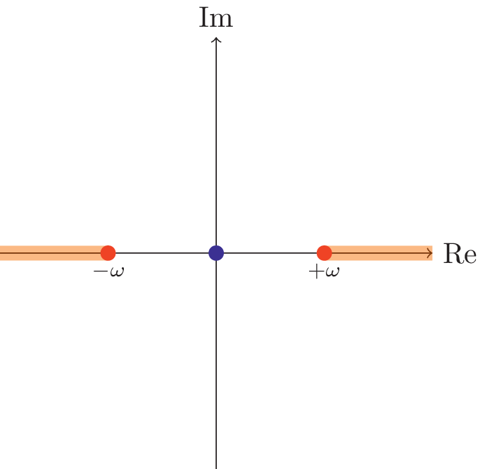


 Open access

