1 Introduction
Originally introduced by Kraichnan (Reference Kraichnan1973) to study energy transfer in inertial turbulence, the triad truncation projects the fluid dynamics onto three Fourier modes with wavevectors
 $\{\boldsymbol{k},\boldsymbol{p},\boldsymbol{q}\}$
such that
 $\boldsymbol{k}+\boldsymbol{p}+\boldsymbol{q}=\mathbf{0}$
. The truncated dynamics of isolated triads differs from the exact fluid flow, failing for example to conserve the topology of the vorticity field (Moffatt Reference Moffatt2014b
). Notwithstanding, the analysis of triadic interactions has yielded important qualitative insights about the direction of energy transfer in externally forced (Waleffe Reference Waleffe1992, Reference Waleffe1993) and magnetohydrodynamic (Lessinnes, Plunian & Carati Reference Lessinnes, Plunian and Carati2009; Linkmann et al.
Reference Linkmann, Berera, McKay and Jäger2016; Linkmann & Dallas Reference Linkmann and Dallas2017) turbulence. Kraichnan (Reference Kraichnan1973) combined the triad truncation with absolute equilibrium considerations to argue against the possibility of an inverse inertial energy cascade in three-dimensional (3-D) helical turbulence (Brissaud et al.
Reference Brissaud, Frisch, Leorat, Lesieur and Mazure1973). Direct numerical simulations of the Navier–Stokes equations (NS) verified later that such turbulence indeed produces only direct energy and helicity cascades (Borue & Orszag Reference Borue and Orszag1997). In the meantime, Waleffe (Reference Waleffe1992, Reference Waleffe1993) formulated his instability assumption, suggesting that there exists a subclass of triads capable of transferring energy to larger scales, but that this subclass is not dominant in isotropic and reflection-invariant turbulence. To amplify the impact of such upward-cascading triads, Biferale, Musacchio & Toschi (Reference Biferale, Musacchio and Toschi2012, Reference Biferale, Musacchio and Toschi2013) studied a projection of the NS equations onto positive helicity states, which breaks reflection invariance and eliminates triads promoting forward energy transfer, and found that inverse energy transfer can develop in such a reduced system. Similar conclusions apply to NS-like equations where the nonlinear term is modified to weight various types of triadic interactions differently (Sahoo, Alexakis & Biferale Reference Sahoo, Alexakis and Biferale2017). New analytical properties of the triadic system continue to be discovered, including pseudo-invariants for a subclass of the interactions (Rathmann & Ditlevsen Reference Rathmann and Ditlevsen2017), with direct implications for externally driven turbulence in passive fluids.
Building on work by Moffatt (Reference Moffatt2014b ), we will extend here the analysis of triad truncations to a class of generalised Navier–Stokes (GNS) equations that constitute effective phenomenological models (Słomka & Dunkel Reference Słomka and Dunkel2017a ,Reference Słomka and Dunkel b ) for intrinsically driven chaotic flows in active fluids (Saintillan & Shelley Reference Saintillan and Shelley2008; Brotto et al. Reference Brotto, Caussin, Lauga and Bartolo2013; Marchetti et al. Reference Marchetti, Joanny, Ramaswamy, Liverpool, Prost, Rao and Simha2013; Giomi Reference Giomi2015), arising from the non-equilibrium stresses exerted by biological or engineered active components (Mendelson et al. Reference Mendelson, Bourque, Wilkening, Anderson and Watkins1999; Dombrowski et al. Reference Dombrowski, Cisneros, Chatkaew, Goldstein and Kessler2004; Howse et al. Reference Howse, Jones, Ryan, Gough, Vafabakhsh and Golestanian2007; Walther & Muller Reference Walther and Muller2008). The recent numerical investigation of a polynomial GNS model (Słomka & Dunkel Reference Słomka and Dunkel2017b ) suggested that active suspensions, such as water-based solutions driven by swimming bacteria (Sokolov et al. Reference Sokolov, Aranson, Kessler and Goldstein2007; Dunkel et al. Reference Dunkel, Heidenreich, Drescher, Wensink, Bär and Goldstein2013) or microtubule networks (Sanchez et al. Reference Sanchez, Chen, DeCamp, Heymann and Dogic2012), can spontaneously break mirror symmetry and develop upward energy transfer even in three dimensions. The analysis below rationalises these findings by identifying a previously unknown cubic invariant, which allows us to classify and contrast the triad dynamics for the classical Euler and the GNS equations. For the GNS case, we show that the asymptotic dynamics reduces to that of a forced rigid body coupled to a particle moving in a magnetic field. For the classical Euler triads, we combine the cubic invariant with the conservation of in-plane energy and enstrophy (Moffatt Reference Moffatt2014b ) to characterise in detail the geometry of the solution space.
1.1 Generalised Navier–Stokes equations for active turbulence
Classical turbulence concerns externally driven flows at high Reynolds number (Frisch Reference Frisch2004; Falkovich & Sreenivasan Reference Falkovich and Sreenivasan2006). By contrast, energy injection in suspensions of self-motile structures (Needleman & Dogic Reference Needleman and Dogic2017) is delocalised and inherently coupled to the flow field. For example, swimming microorganisms (Mendelson et al.
Reference Mendelson, Bourque, Wilkening, Anderson and Watkins1999; Dombrowski et al.
Reference Dombrowski, Cisneros, Chatkaew, Goldstein and Kessler2004; Pedley Reference Pedley2010; Ishikawa et al.
Reference Ishikawa, Yoshida, Ueno, Wiedeman, Imai and Yamaguchi2011; Dunkel et al.
Reference Dunkel, Heidenreich, Drescher, Wensink, Bär and Goldstein2013) stir the surrounding fluid, but also respond to the flow field and interact through the fluid. Similar flow-dependent forcing mechanisms are present in suspensions of artificial microswimmers (Howse et al.
Reference Howse, Jones, Ryan, Gough, Vafabakhsh and Golestanian2007; Walther & Muller Reference Walther and Muller2008; Bricard et al.
Reference Bricard, Caussin, Desreumaux, Dauchot and Bartolo2013) or adenosine triphosphate-driven microtubule networks (Sanchez et al.
Reference Sanchez, Chen, DeCamp, Heymann and Dogic2012). When the concentration of such active objects is sufficiently high, self-sustained chaotic flow patterns emerge; this phenomenon is commonly referred to as active turbulence nowadays (Wolgemuth Reference Wolgemuth2008; Wensink et al.
Reference Wensink, Dunkel, Heidenreich, Drescher, Goldstein, Löwen and Yeomans2012; Bratanov, Jenko & Frey Reference Bratanov, Jenko and Frey2015; Giomi Reference Giomi2015; Urzay, Doostmohammadi & Yeomans Reference Urzay, Doostmohammadi and Yeomans2017). A striking difference between classical and active turbulence is that the latter often exhibits characteristic scales, leading to a preferred eddy size (Sokolov et al.
Reference Sokolov, Aranson, Kessler and Goldstein2007; Sanchez et al.
Reference Sanchez, Chen, DeCamp, Heymann and Dogic2012; Sokolov & Aranson Reference Sokolov and Aranson2012; Wensink et al.
Reference Wensink, Dunkel, Heidenreich, Drescher, Goldstein, Löwen and Yeomans2012; Dunkel et al.
Reference Dunkel, Heidenreich, Drescher, Wensink, Bär and Goldstein2013). A minimal phenomenological model combining scale selection with flow-dependent driving is given by the higher-order GNS equations for the velocity field
 $\boldsymbol{v}(\boldsymbol{x},t)$
(Słomka & Dunkel Reference Słomka and Dunkel2017a
,Reference Słomka and Dunkel
b
)
 $$\begin{eqnarray}\displaystyle \unicode[STIX]{x1D735}\boldsymbol{\cdot }\boldsymbol{v}=0, & & \displaystyle\end{eqnarray}$$

 $p$
is the pressure, and the higher-order stress tensor

with
 $\unicode[STIX]{x1D6FB}^{2n}\equiv (\unicode[STIX]{x1D6FB}^{2})^{n}$
,
 $n\geqslant 2$
, accounts effectively for both passive contributions from the intrinsic solvent fluid viscosity and active contributions representing the stresses exerted by the microswimmers on the fluid. By construction, equations (1.1) and (1.2) neglect non-advective nonlinearities such as nematic alignment interactions that become important at very high swimmer concentrations. Related higher-order Navier–Stokes models have been studied previously in the context of soft-mode turbulence and seismic waves (Beresnev & Nikolaevskiy Reference Beresnev and Nikolaevskiy1993; Tribelsky & Tsuboi Reference Tribelsky and Tsuboi1996; Tribelsky Reference Tribelsky2008) so that the considerations below may extend to these systems as well. On a periodic cubic domain, the Fourier representation of (1.1) and (1.2) reads
 $$\begin{eqnarray}\displaystyle \left[\frac{\unicode[STIX]{x2202}}{\unicode[STIX]{x2202}t}+\unicode[STIX]{x1D709}(k)\right]\hat{v}_{a}(\boldsymbol{k},t)=-\text{i}\mathop{\sum }_{\boldsymbol{k}+\boldsymbol{p}+\boldsymbol{q}=\mathbf{0}}P_{ab}(\boldsymbol{k})q_{c}\hat{v}_{c}^{\ast }(\boldsymbol{p},t)\hat{v}_{b}^{\ast }(\boldsymbol{q},t), & & \displaystyle\end{eqnarray}$$
where
 $k=|\boldsymbol{k}|$
, the projector
 $P_{ab}=\unicode[STIX]{x1D6FF}_{ab}-k_{a}k_{b}/k^{2}$
enforces incompressibility and the dispersion relation is given by the polynomial
 $$\begin{eqnarray}\displaystyle \unicode[STIX]{x1D709}(k)=\unicode[STIX]{x1D6E4}_{0}k^{2}+\unicode[STIX]{x1D6E4}_{2}k^{4}+\unicode[STIX]{x1D6E4}_{4}k^{6}, & & \displaystyle\end{eqnarray}$$
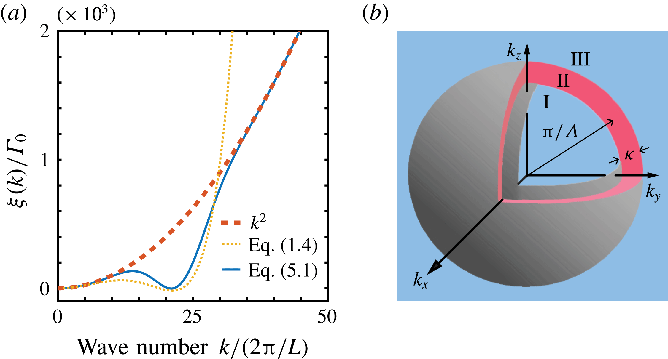
see figure 1(a). Microswimmer activity is modelled by letting
 $\unicode[STIX]{x1D6E4}_{2}<0$
, which introduces a band of linearly unstable modes with
 $\unicode[STIX]{x1D709}(k)<0$
, while
 $\unicode[STIX]{x1D6E4}_{0}>0$
and
 $\unicode[STIX]{x1D6E4}_{4}>0$
represent damping at large and small scales with
 $\unicode[STIX]{x1D709}(k)>0$
. The most unstable wavenumber
 $k_{\unicode[STIX]{x1D6EC}}$
determines the typical eddy size
 $\unicode[STIX]{x1D6EC}=\unicode[STIX]{x03C0}/k_{\unicode[STIX]{x1D6EC}}$
, the corresponding growth rate sets the time scale
 $\unicode[STIX]{x1D70F}=-\unicode[STIX]{x1D709}(k_{\unicode[STIX]{x1D6EC}})^{-1}$
, and we denote by
 $\unicode[STIX]{x1D705}$
the bandwidth of the unstable modes, see figure 1(b). The parameters
 $(\unicode[STIX]{x1D6EC},\unicode[STIX]{x1D70F},\unicode[STIX]{x1D705})$
, uniquely determined by
 $(\unicode[STIX]{x1D6E4}_{0},\unicode[STIX]{x1D6E4}_{2},\unicode[STIX]{x1D6E4}_{4})$
, characterise the resulting flow structures and can be inferred from experimental data (Słomka & Dunkel Reference Słomka and Dunkel2017b
). Numerical simulations showed that the polynomial GNS model defined by (1.3) and (1.4) exhibits spontaneous mirror symmetry breaking by developing helical flow structures that are statistically close to Beltrami fields. The strength of the symmetry breaking is controlled by the active bandwidth
 $\unicode[STIX]{x1D705}$
, corresponding to the red domain in figure 1(b). For sufficiently small
 $\unicode[STIX]{x1D705}\ll \unicode[STIX]{x1D6EC}^{-1}$
, an upward energy transfer develops in an otherwise homogeneous and isotropic active turbulence (Słomka & Dunkel Reference Słomka and Dunkel2017b
).
(a) Dispersion relations
 $\unicode[STIX]{x1D709}(k)$
for the polynomial GNS model (1.4) and the Gaussian GNS model (5.1). Modes with
 $\unicode[STIX]{x1D709}(k)<0$
define the energy injection and scale selection domain typical of active turbulence. (b) Illustration of the key model parameters in 3-D Fourier space. The spectral bandwidth
 $\unicode[STIX]{x1D705}$
defines the width of the unstable domain II (red), which is localised around the characterised vortex-scale
 $\unicode[STIX]{x1D6EC}$
and separates dissipative Fourier modes at large (region I) and small scales (region III); reproduced with permission from Słomka & Dunkel (Reference Słomka and Dunkel2017b
).

1.2 Triad interactions in active turbulence
In this work, we investigate analytically and numerically the dynamical system arising from the triad truncation of (1.3). In contrast to the approach typically adopted when studying the inertial energy transfer in classical turbulence, our analysis does not neglect the linear term
 $\unicode[STIX]{x1D709}(k)$
, although we will later discuss the implications for the classical case
 $\unicode[STIX]{x1D709}(k)\equiv 0$
as well. Specifically, we focus on the subclass of all possible triad interactions in which one or two ‘legs’ lie in the energy injection range, while the remaining legs are dissipative. We refer to such triads as ‘active triads’, to distinguish them from the ‘classical triads’ for which
 $\unicode[STIX]{x1D709}(k)\equiv 0$
. Utilising a previously unrecognised cubic invariant, we show that the resulting triad dynamics is asymptotically equivalent to a coupled system of a rigid body and a particle moving in a magnetic field. This analogy allows us to classify the active triads by their asymptotic stability: triads forced at the small or large scale are unstable and increase energy and helicity exponentially, whereas triads forced at the intermediate scale are stable and develop a limit cycle. This asymptotic behaviour of the active triads is in stark contrast to the classical triadic dynamics, for which the rigid-body analogy does not hold in general but whose solutions one can classify using the cubic invariant. For the untruncated system (1.3), it is plausible that unstable active triads dominate the initial relaxation characterised by helicity growth, whereas stable active triads determine the subsequent statistically stationary stage. To support this hypothesis, and to demonstrate that the predictions of the polynomial model generalise to a broader class of flow-dependent forcing schemes, we will also consider a non-polynomial active turbulence model (5.1) which combines the usual viscous dissipation
 ${\sim}\unicode[STIX]{x1D6E4}_{0}k^{2}$
with a Gaussian forcing term, see blue solid curve in figure 1(a). We will use direct numerical simulations to show that the Gaussian activity model develops strongly aligned steady-state velocity and vorticity fields and an inverse energy cascade. The upward energy transfer is non-inertial, yet the weak dependence of the energy flux on the wavenumber generates energy spectra that approximately follow
 $-5/3$
scaling (Kolmogorov Reference Kolmogorov1941) at large wavelengths. These results suggest that Beltrami-type flows and an inverse energy cascade are generic features of 3-D active turbulence models with flow-dependent narrow spectral forcing.
2 Triad truncation and its asymptotic dynamics
We introduce the triad truncation of (1.3) for
 $\unicode[STIX]{x1D709}(k)\neq 0$
, extending the approach of Kraichnan (Reference Kraichnan1973) who considered the case
 $\unicode[STIX]{x1D709}(k)\equiv 0$
corresponding to the inertial range approximation. We adopt the notation and build on the results of Moffatt (Reference Moffatt2014b
).
2.1 Truncation
Triad truncation is the projection of the dynamics (1.3) onto three Fourier modes
 $\{\hat{\boldsymbol{v}}(\boldsymbol{k},t),\hat{\boldsymbol{v}}(\boldsymbol{p},t),\hat{\boldsymbol{v}}(\boldsymbol{q},t)\}$
such that
 $\boldsymbol{k}+\boldsymbol{p}+\boldsymbol{q}=\mathbf{0}$
. The truncation is a first step beyond full linearisation (which completely decouples the Fourier modes), to keep the smallest non-trivial portion of the quadratic nonlinearity. The velocity field reduces to
 $$\begin{eqnarray}\displaystyle \boldsymbol{v}(\boldsymbol{x},t)=\hat{\boldsymbol{v}}(\boldsymbol{k},t)\text{e}^{\text{i}\boldsymbol{k}\boldsymbol{\cdot }\boldsymbol{x}}+\hat{\boldsymbol{v}}(\boldsymbol{p},t)\text{e}^{\text{i}\boldsymbol{p}\boldsymbol{\cdot }\boldsymbol{x}}+\hat{\boldsymbol{v}}(\boldsymbol{q},t)\text{e}^{\text{i}\boldsymbol{q}\boldsymbol{\cdot }\boldsymbol{x}}+\text{c.c.}, & & \displaystyle\end{eqnarray}$$
where c.c. denotes complex conjugate terms which ensure that
 $\boldsymbol{v}(\boldsymbol{x},t)$
is real. Since the triad
 $\{\boldsymbol{k},\boldsymbol{p},\boldsymbol{q}\}$
forms a triangle, it may be taken to lie in the
 $(x,y)$
-plane by rotating the coordinate system, implying that the velocity field is independent of the spatial variable
 $z$
. This allows one to introduce a streamfunction
 $\unicode[STIX]{x1D713}$
and write the velocity field as
 $\boldsymbol{v}=(\unicode[STIX]{x2202}\unicode[STIX]{x1D713}/\unicode[STIX]{x2202}y,-\unicode[STIX]{x2202}\unicode[STIX]{x1D713}/\unicode[STIX]{x2202}x,v_{z})$
. Thus, rather than working with the representation (2.1), it is more convenient to introduce the triadic expansions of the scalars
 $\unicode[STIX]{x1D713}$
and
 $v_{z}$
(Moffatt Reference Moffatt2014b
)
 $$\begin{eqnarray}\displaystyle \unicode[STIX]{x1D713}(x,y,t) & = & \displaystyle A_{k}(t)\text{e}^{\text{i}\boldsymbol{k}\boldsymbol{\cdot }\boldsymbol{x}}+A_{p}(t)\text{e}^{\text{i}\boldsymbol{p}\boldsymbol{\cdot }\boldsymbol{x}}+A_{q}(t)\text{e}^{\text{i}\boldsymbol{q}\boldsymbol{\cdot }\boldsymbol{x}}+\text{c.c.},\end{eqnarray}$$
 $$\begin{eqnarray}\displaystyle v_{z}(x,y,t) & = & \displaystyle B_{k}(t)\text{e}^{\text{i}\boldsymbol{k}\boldsymbol{\cdot }\boldsymbol{x}}+B_{p}(t)\text{e}^{\text{i}\boldsymbol{p}\boldsymbol{\cdot }\boldsymbol{x}}+B_{q}(t)\text{e}^{\text{i}\boldsymbol{q}\boldsymbol{\cdot }\boldsymbol{x}}+\text{c.c.}\end{eqnarray}$$
 $\boldsymbol{A}=(A_{k},A_{p},A_{q})$
and
 $\boldsymbol{B}=(B_{k},B_{p},B_{q})$
results in the following system of coupled differential equations
 $$\begin{eqnarray}\displaystyle \unicode[STIX]{x1D644}\dot{\boldsymbol{A}}+\unicode[STIX]{x1D63F}\unicode[STIX]{x1D644}\boldsymbol{A} & = & \displaystyle 2\unicode[STIX]{x1D6E5}(\unicode[STIX]{x1D644}\boldsymbol{A}^{\ast }\times \boldsymbol{A}^{\ast }),\end{eqnarray}$$
 $$\begin{eqnarray}\displaystyle \dot{\boldsymbol{B}}+\unicode[STIX]{x1D63F}\boldsymbol{B} & = & \displaystyle 2\unicode[STIX]{x1D6E5}(\boldsymbol{B}^{\ast }\times \boldsymbol{A}^{\ast }),\end{eqnarray}$$
 $\unicode[STIX]{x1D6E5}=(k_{x}p_{y}-k_{y}p_{x})/2$
is the area of the triangle formed by
 $\{\boldsymbol{k},\boldsymbol{p},\boldsymbol{q}\}$
and
 $$\begin{eqnarray}\displaystyle \unicode[STIX]{x1D644}=\text{diag}(k^{2},p^{2},q^{2}),\quad \unicode[STIX]{x1D63F}=\text{diag}(\unicode[STIX]{x1D709}(k),\unicode[STIX]{x1D709}(p),\unicode[STIX]{x1D709}(q)). & & \displaystyle\end{eqnarray}$$
The positive and negative entries of
 $\unicode[STIX]{x1D63F}$
represent dissipation and forcing of the three modes, respectively. The key difference between the system (2.3) and the classical triad truncation is the matrix
 $\unicode[STIX]{x1D63F}$
, which vanishes in the latter case. The typically studied case
 $\unicode[STIX]{x1D63F}=\text{0}$
is suitable for the inertial range considerations in classical turbulence and arises formally from the truncation of the inviscid Euler equation. In the context of active turbulence, we are interested in the case
 $\unicode[STIX]{x1D63F}\neq \text{0}$
.
Energy
 $E$
and helicity
 $H$
of the triad are given by Moffatt (Reference Moffatt2014b
)
 $$\begin{eqnarray}\displaystyle 2E & = & \displaystyle k^{2}|A_{k}|^{2}+p^{2}|A_{p}|^{2}+q^{2}|A_{q}|^{2}+|\boldsymbol{B}|^{2},\end{eqnarray}$$
 $$\begin{eqnarray}\displaystyle H & = & \displaystyle \unicode[STIX]{x1D644}\boldsymbol{A}\boldsymbol{\cdot }\boldsymbol{B}^{\ast }+\unicode[STIX]{x1D644}\boldsymbol{A}^{\ast }\boldsymbol{\cdot }\boldsymbol{B}.\end{eqnarray}$$
 $$\begin{eqnarray}\displaystyle \text{tr}(\unicode[STIX]{x1D63F})=\unicode[STIX]{x1D709}(k)+\unicode[STIX]{x1D709}(p)+\unicode[STIX]{x1D709}(q)>0. & & \displaystyle\end{eqnarray}$$
Since in a finite spatial domain the number of active modes with
 $\unicode[STIX]{x1D709}(k)<0$
is finite, this condition is always satisfied for triads with at most two active legs, say
 $\unicode[STIX]{x1D709}(p)<0$
and
 $\unicode[STIX]{x1D709}(k)<0$
but
 $\unicode[STIX]{x1D709}(q)>0$
, provided the forcing is sufficiently weak.
Finally, we express the helical decomposition (Constantin & Majda Reference Constantin and Majda1988; Waleffe Reference Waleffe1992; Alexakis Reference Alexakis2017; Biferale, Buzzicotti & Linkmann Reference Biferale, Buzzicotti and Linkmann2017) in terms of
 $\boldsymbol{A}$
and
 $\boldsymbol{B}$
. Since the triad lies in the
 $(x,y)$
-plane, the curl eigenmodes can be taken as
 $$\begin{eqnarray}\displaystyle \boldsymbol{h}_{\pm }(\boldsymbol{k})=\hat{\boldsymbol{z}}\times \hat{\boldsymbol{k}}\pm \text{i}\hat{\boldsymbol{z}}=(-k_{y},k_{x},\pm \text{i}k)/k. & & \displaystyle\end{eqnarray}$$
Projecting
 $\hat{\boldsymbol{v}}(\boldsymbol{k})$
onto these eigenmodes gives the helical decomposition
 $$\begin{eqnarray}\displaystyle a_{\pm }(\boldsymbol{k})=\frac{1}{2}\boldsymbol{h}^{\pm }(\boldsymbol{k})^{\ast }\boldsymbol{\cdot }\hat{\boldsymbol{v}}(\boldsymbol{k})=-\frac{\text{i}}{2}(kA_{k}\pm B_{k}). & & \displaystyle\end{eqnarray}$$
Analogous expressions hold for
 $\boldsymbol{p}$
and
 $\boldsymbol{q}$
.
2.2 Asymptotic rigid-body dynamics: a cubic invariant
Since, according to (2.3), the dynamics of
 $\boldsymbol{A}$
affects
 $\boldsymbol{B}$
, but not vice versa, we study (2.3a
) first. In components, equation (2.3a
) reads
 $$\begin{eqnarray}\displaystyle \left.\begin{array}{@{}c@{}}k^{2}{\dot{A}}_{k}+\unicode[STIX]{x1D709}(k)k^{2}A_{k}=2\unicode[STIX]{x1D6E5}(p^{2}-q^{2})A_{p}^{\ast }A_{q}^{\ast }\\ p^{2}{\dot{A}}_{p}+\unicode[STIX]{x1D709}(p)p^{2}A_{p}=2\unicode[STIX]{x1D6E5}(q^{2}-k^{2})A_{q}^{\ast }A_{k}^{\ast }\\ q^{2}{\dot{A}}_{q}+\unicode[STIX]{x1D709}(q)q^{2}A_{q}=2\unicode[STIX]{x1D6E5}(k^{2}-p^{2})A_{k}^{\ast }A_{p}^{\ast }.\end{array}\right\} & & \displaystyle\end{eqnarray}$$
This system has the following three properties:
-
(i) If the initial conditions are real, then
 $\boldsymbol{A}(t)$
is real for all
$t$
. In this case, equation (2.3a
) reduces to the Euler equations for the rotation of a rigid body.
-
(ii) The change of variables given by the constant phase shifts
$(\unicode[STIX]{x1D719}_{k},\unicode[STIX]{x1D719}_{p},\unicode[STIX]{x1D719}_{q})$
(2.10)leaves the equations (2.9) unchanged.
$$\begin{eqnarray}\displaystyle (A_{k}^{\prime },A_{p}^{\prime },A_{q}^{\prime })=(A_{k}\text{e}^{-\text{i}\unicode[STIX]{x1D719}_{k}},A_{p}\text{e}^{-\text{i}\unicode[STIX]{x1D719}_{p}},A_{q}\text{e}^{-\text{i}\unicode[STIX]{x1D719}_{q}})\quad \text{where }\unicode[STIX]{x1D719}_{k}+\unicode[STIX]{x1D719}_{p}+\unicode[STIX]{x1D719}_{q}=0 & & \displaystyle\end{eqnarray}$$
-
(iii) The following identity holds
(2.11)where
$$\begin{eqnarray}\displaystyle \operatorname{Im}(A_{k}A_{p}A_{q})=|A_{k}||A_{p}||A_{q}|\sin (\unicode[STIX]{x1D719}_{k}+\unicode[STIX]{x1D719}_{p}+\unicode[STIX]{x1D719}_{q})=C\,\text{exp}[-\text{tr}(\unicode[STIX]{x1D63F})t], & & \displaystyle\end{eqnarray}$$
$C=\operatorname{Im}[A_{k}(0)A_{p}(0)A_{q}(0)]$
and we introduced polar representations
$A_{k}=|A_{k}|\text{e}^{\text{i}\unicode[STIX]{x1D719}_{k}}$
, etc. Equation (2.11) also implies that (2.12)where we introduced the real and imaginary components,
$$\begin{eqnarray}\displaystyle \operatorname{Im}(k^{2}{\dot{A}}_{k}^{\ast }A_{k})=k^{2}\det \left[\begin{array}{@{}cc@{}}\operatorname{Re}{\dot{A}}_{k} & \operatorname{Re}A_{k}\\ \operatorname{Im}{\dot{A}}_{k} & \operatorname{Im}A_{k}\end{array}\right]=2\unicode[STIX]{x1D6E5}(p^{2}-q^{2})C\,\text{exp}[-\text{tr}(\unicode[STIX]{x1D63F})t], & & \displaystyle\end{eqnarray}$$
$A_{k}=\operatorname{Re}A_{k}+\text{i}\operatorname{Im}A_{k}$
. Analogous expressions hold for
$A_{p}$
and
$A_{q}$
. Equation (2.12) has a useful geometrical interpretation: it gives the areal velocity (rate at which area is swept out) as a function of time of the complex trajectory traced out by the mode
$A_{k}(t)$
. Since we focus on triads with
$\text{tr}(\unicode[STIX]{x1D63F})>0$
, this immediately implies that the mode eventually vanishes, becomes stationary, or its trajectory approaches a line through the origin.








The property (i) was pointed out in Waleffe (Reference Waleffe1992), Moffatt (Reference Moffatt2014b
). The second property is easily verified by direct substitution. To derive the last property, multiply the first equation in (2.9) by
 $A_{p}A_{q}$
, etc., to obtain
 $$\begin{eqnarray}\displaystyle \left.\begin{array}{@{}c@{}}k^{2}{\dot{A}}_{k}A_{p}A_{q}+\unicode[STIX]{x1D709}(k)k^{2}A_{k}A_{p}A_{q}=2\unicode[STIX]{x1D6E5}(p^{2}-q^{2})|A_{p}|^{2}|A_{q}|^{2}\\ p^{2}A_{k}{\dot{A}}_{p}A_{q}+\unicode[STIX]{x1D709}(p)p^{2}A_{k}A_{p}A_{q}=2\unicode[STIX]{x1D6E5}(q^{2}-k^{2})|A_{q}|^{2}|A_{k}|^{2}\\ q^{2}A_{k}A_{p}{\dot{A}}_{q}+\unicode[STIX]{x1D709}(q)q^{2}A_{k}A_{p}A_{q}=2\unicode[STIX]{x1D6E5}(k^{2}-p^{2})|A_{k}|^{2}|A_{p}|^{2}.\end{array}\right\} & & \displaystyle\end{eqnarray}$$
Subtract from each equation its complex conjugate and add the resulting expressions
 $$\begin{eqnarray}\displaystyle {\dot{A}}_{k}A_{p}A_{q}+A_{k}{\dot{A}}_{p}A_{q}+A_{k}A_{p}{\dot{A}}_{q}+[\unicode[STIX]{x1D709}(k)+\unicode[STIX]{x1D709}(p)+\unicode[STIX]{x1D709}(q)]A_{k}A_{p}A_{q}-\text{c.c.}=0. & & \displaystyle\end{eqnarray}$$
Now use the chain rule and substitute
 $\unicode[STIX]{x1D709}(k)+\unicode[STIX]{x1D709}(p)+\unicode[STIX]{x1D709}(q)=\text{tr}(\unicode[STIX]{x1D63F})$
 $$\begin{eqnarray}\displaystyle \frac{\text{d}}{\text{d}t}(A_{k}A_{p}A_{q}-A_{k}^{\ast }A_{p}^{\ast }A_{q}^{\ast })=-\text{tr}(\unicode[STIX]{x1D63F})(A_{k}A_{p}A_{q}-A_{k}^{\ast }A_{p}^{\ast }A_{q}^{\ast }). & & \displaystyle\end{eqnarray}$$
Property (iii) then follows from integrating this first-order equation. To derive (2.12), multiply the first equation in (2.9) by
 $A_{k}^{\ast }$
, etc., subtract from each such obtained equation its complex conjugate and then use (2.11).
We note that (iii) also implies that
 $\operatorname{Im}(A_{k}A_{p}A_{q})$
is conserved in the inertial range of classical turbulence, where
 $\unicode[STIX]{x1D63F}=\text{0}$
holds. This adds a cubic invariant to a list of quadratic invariants of the classical triadic system (Waleffe Reference Waleffe1992; Moffatt Reference Moffatt2014b
; Rathmann & Ditlevsen Reference Rathmann and Ditlevsen2017). In § 4 we combine the cubic invariant with the conservation of in-plane energy and enstrophy (Moffatt Reference Moffatt2014b
) to obtain a detailed geometric classification of the solutions of the system (2.3a
) when
 $\unicode[STIX]{x1D63F}=\text{0}$
.
2.3 Asymptotic dynamics: rigid body and particle in a magnetic field
We use the properties (i)–(iii) to argue that the dynamics (2.9) is asymptotically equivalent to that of a forced rigid body with principal moments of inertia
 $(k^{2},p^{2},q^{2})$
. Since we consider triads for which
 $\text{tr}(\unicode[STIX]{x1D63F})>0$
, equation (2.11) suggests that the phase curves of (2.9) approach the following algebraic subset
 $S$
at an exponential rate
 $$\begin{eqnarray}\displaystyle \operatorname{Im}(A_{k}A_{p}A_{q})=|A_{k}||A_{p}||A_{q}|\sin (\unicode[STIX]{x1D719}_{k}+\unicode[STIX]{x1D719}_{p}+\unicode[STIX]{x1D719}_{q})=0. & & \displaystyle\end{eqnarray}$$
For the purposes of asymptotic analysis, we assume it is sufficient to consider initial conditions
 $\boldsymbol{A}(0)$
lying on the attractor
 $S$
. There are two possibilities:
 $$\begin{eqnarray}\displaystyle |A_{i}|=0\quad \text{for some }i\in \{k,p,q\}\quad \text{or}\quad \unicode[STIX]{x1D719}_{k}+\unicode[STIX]{x1D719}_{p}+\unicode[STIX]{x1D719}_{q}=n\unicode[STIX]{x03C0}. & & \displaystyle\end{eqnarray}$$
Regardless which of the three conditions
 $\boldsymbol{A}(0)$
satisfies, the property (ii) implies it is always possible to perform a change of variables that makes
 $\boldsymbol{A}(0)$
a real vector without altering the dynamics (2.9). But then it follows from property (i) that
 $\boldsymbol{A}(t)$
is real for all
 $t$
. The asymptotic dynamics of the complex system (2.9) therefore becomes effectively equivalent to that of the real system
 $$\begin{eqnarray}\displaystyle \unicode[STIX]{x1D644}\dot{\unicode[STIX]{x1D74E}}+\unicode[STIX]{x1D63F}\unicode[STIX]{x1D644}\unicode[STIX]{x1D74E}=\unicode[STIX]{x1D644}\unicode[STIX]{x1D74E}\times \unicode[STIX]{x1D74E}, & & \displaystyle\end{eqnarray}$$
where
 $\unicode[STIX]{x1D74E}=(\unicode[STIX]{x1D714}_{k},\unicode[STIX]{x1D714}_{p},\unicode[STIX]{x1D714}_{q})$
is a real vector. Equation (2.18) has the structure of the Euler equations for a forced rigid body with inertia tensor
 $\unicode[STIX]{x1D644}$
and angular velocity
 $\unicode[STIX]{x1D74E}$
. When a triadic leg lies in the active or passive range, the rigid body is either forced or damped along the corresponding axis of inertia. Importantly, the forcing/damping is proportional to the component of angular momentum
 $\unicode[STIX]{x1D644}\unicode[STIX]{x1D74E}$
along that axis. The system (2.18) admits exact solutions corresponding to exponential growth or decay of rotations about one principal axis only, for example
 $\unicode[STIX]{x1D74E}=c(\text{e}^{-D_{kk}t},0,0)$
.
We now focus on the asymptotic dynamics of the system (2.3b
) for
 $\boldsymbol{B}$
. Since by the above analysis
 $\boldsymbol{A}$
can be eventually taken to be the real vector
 $\unicode[STIX]{x1D74E}$
, the real and imaginary parts of
 $\boldsymbol{B}$
asymptotically decouple into two equations
 $$\begin{eqnarray}\displaystyle \operatorname{Re}\dot{\boldsymbol{B}}+\unicode[STIX]{x1D63F}\operatorname{Re}\boldsymbol{B} & = & \displaystyle \operatorname{Re}\boldsymbol{B}\times \unicode[STIX]{x1D74E},\end{eqnarray}$$
 $$\begin{eqnarray}\displaystyle \operatorname{Im}\dot{\boldsymbol{B}}+\unicode[STIX]{x1D63F}\operatorname{Im}\boldsymbol{B} & = & \displaystyle -\operatorname{Im}\,\boldsymbol{B}\times \unicode[STIX]{x1D74E}.\end{eqnarray}$$
 $\boldsymbol{u}=\operatorname{Re}\boldsymbol{B}$
and charge
 $+1$
moving in a magnetic field
 $\unicode[STIX]{x1D74E}$
. The second equation describes an analogous dynamics with velocity
 $\operatorname{Im}\boldsymbol{B}$
and charge
 $-1$
. Since for real-valued
 $\unicode[STIX]{x1D74E}$
the helicity (2.5b
) is determined by the real part of
 $\boldsymbol{B}$
, we may conclude that the triadic system (2.3), in the long-time limit, becomes equivalent to the following equations for the real vectors
 $\unicode[STIX]{x1D74E}$
and
 $\boldsymbol{u}$
 $$\begin{eqnarray}\displaystyle \unicode[STIX]{x1D644}\dot{\unicode[STIX]{x1D74E}}+\unicode[STIX]{x1D63F}\unicode[STIX]{x1D644}\unicode[STIX]{x1D74E} & = & \displaystyle \unicode[STIX]{x1D644}\unicode[STIX]{x1D74E}\times \unicode[STIX]{x1D74E},\end{eqnarray}$$
 $$\begin{eqnarray}\displaystyle \dot{\boldsymbol{u}}+\unicode[STIX]{x1D63F}\boldsymbol{u} & = & \displaystyle \boldsymbol{u}\times \unicode[STIX]{x1D74E}.\end{eqnarray}$$
 $\unicode[STIX]{x1D74E}$
of the forced rigid body acts as a magnetic field for a forced particle moving with velocity
 $\boldsymbol{u}$
. In this notation, the triad helicity is the dot product between the rigid-body angular momentum and the particle velocity
 $$\begin{eqnarray}\displaystyle H=2\unicode[STIX]{x1D644}\unicode[STIX]{x1D74E}\boldsymbol{\cdot }\boldsymbol{u}. & & \displaystyle\end{eqnarray}$$
Thus, the helicity is positive when the particle moves in the direction of the angular momentum and negative when it moves in the opposite direction.
3 Triad classification
We would like to classify active triads according to their long-time behaviour; we call triads stable or unstable if they tend to produce bounded or unbounded energy, respectively. It is useful to develop first an intuitive understanding based on the asymptotic correspondence with the ‘rigid body and a particle in a magnetic field’ system (2.20). Subsequently, we will confirm the intuitive picture through explicit numerical simulations.
Without forcing,
 $\unicode[STIX]{x1D63F}=\text{0}$
in (2.20a
), the rigid-body dynamics admits three fixed points, which correspond to constant angular velocity rotation about one of the three principal axes. The rotations about the small
 $(p^{2})$
or large
 $(q^{2})$
axis are stable fixed points, whereas rotation about the middle axis
 $(k^{2})$
is unstable (Arnold Reference Arnold1989). With forcing,
 $\unicode[STIX]{x1D63F}\neq \text{0}$
, the linear part of (2.20a
) promotes exponential growth of the mode for which
 $D_{ii}<0$
and damping of the remaining modes. It is conceivable that, when combined with the Eulerian nonlinearity, the coupled dynamical system (2.20), and hence the system (2.3), becomes unstable (asymptotically produces infinite energy) when the rigid body is forced at the small or large principal axis, for in this case the nonlinearity does not counteract the exponential growth. However, when forced at the middle principal axis, the nonlinearity should induce motion about the remaining axes. Since these axes are dissipative, the system should soon realign with the middle principal axis, until the nonlinearity becomes dominant again, and so on. Numerical investigations presented in § 3.2 suggest that the dynamics (2.3a
) indeed approaches a limit cycle, although we do not rule out the possibility of more complicated attractors for some particular triads and parameters
 $D_{ii}$
.
In all numerical simulations of (2.3) we use the polynomial dispersion relation
 $\unicode[STIX]{x1D709}(k)$
given by (1.4) with parameters
 $(\unicode[STIX]{x1D6E4}_{0},\unicode[STIX]{x1D6E4}_{2},\unicode[STIX]{x1D6E4}_{4})$
corresponding to the characteristic triple (
 $\unicode[STIX]{x1D6EC}=75~\unicode[STIX]{x03BC}$
m,
 $\unicode[STIX]{x1D70F}=6.4$
s,
 $\unicode[STIX]{x1D705}=8.4~\text{mm}^{-1}$
), as studied in Słomka & Dunkel (Reference Słomka and Dunkel2017b
). For time stepping, we use the classical Runge–Kutta method (RK4).
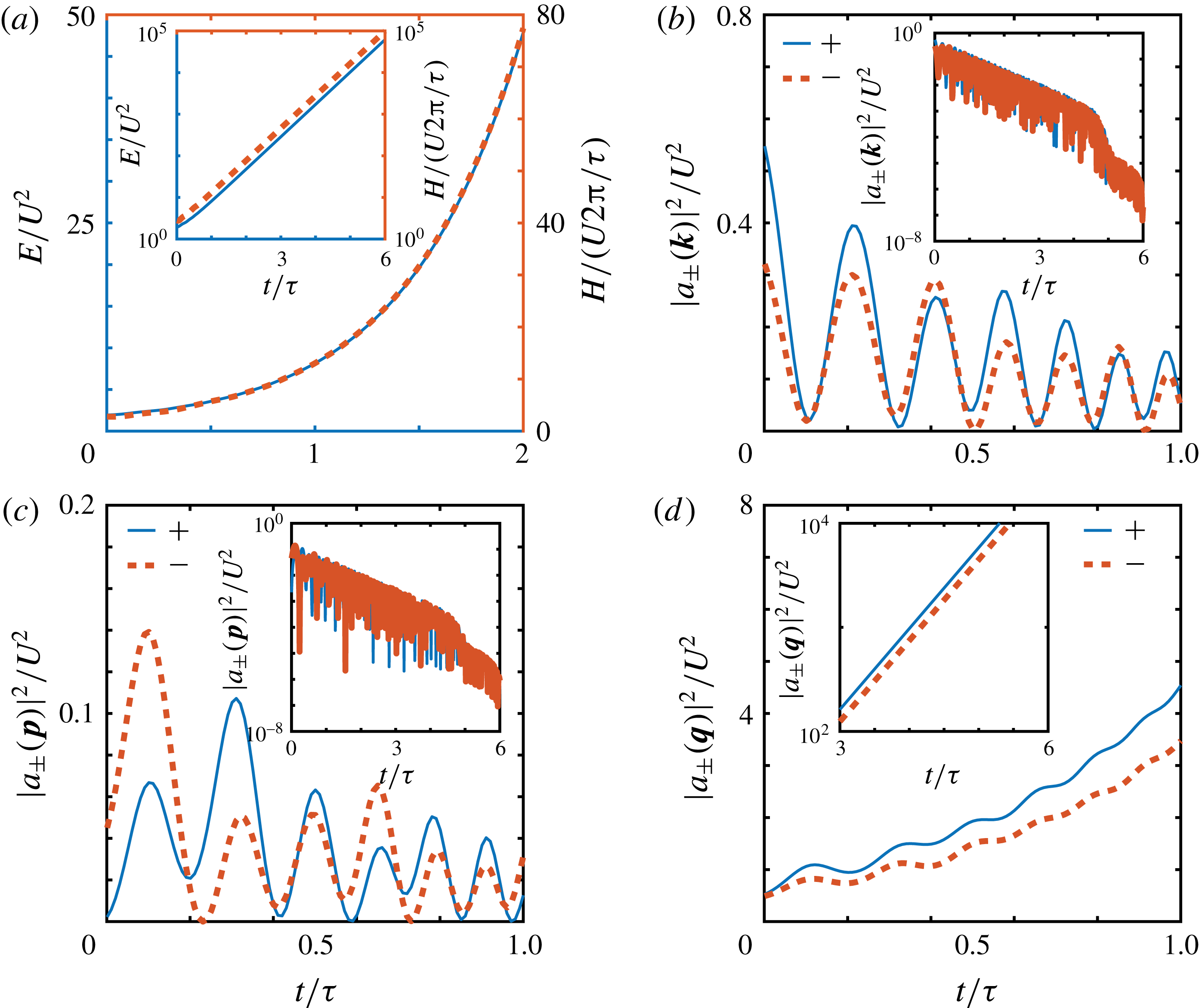
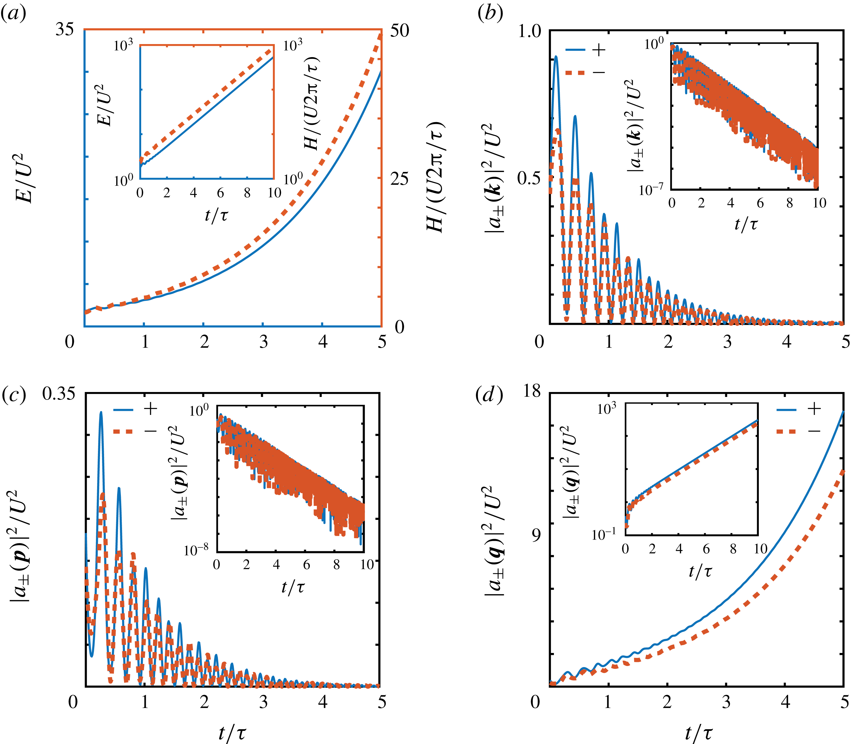
Numerical simulations of (2.3) with polynomial dispersion (1.4) initiated with random complex initial conditions show that active triads (
 $p<k<q$
) are unstable when forced at large wavenumbers
 $q$
. Energy and helicity increase exponentially (a), reflecting the exponential growth of the forced helical mode (d) and underdamped decay of the passive helical modes (b,c). Parameters:
 $\{\boldsymbol{k},\boldsymbol{p},\boldsymbol{q}\}=[(-5,9,0),(1,2,0),(4,-11,0)]$
, box size
 $L=24\unicode[STIX]{x1D6EC}$
.

3.1 Unstable triads: rigid body forced at the small or large principal axis
Suppose the triadic system is forced at the small scale
 $q$
, implying that
 $D_{qq}<0$
but
 $D_{kk}>0$
and
 $D_{pp}>0$
in (2.3). The rigid-body correspondence suggests the
 $q$
-mode should become unstable as the exponential growth and the nonlinearity reinforce each other. Indeed,
 $\boldsymbol{A}=c(0,0,\text{e}^{-D_{qq}t})$
is an exact unstable solution of (2.3a
). The remaining part of the triadic system (2.3) is the equation (2.3b
) for
 $\boldsymbol{B}$
. In the long-time limit, when
 $\boldsymbol{A}\rightarrow c(0,0,\text{e}^{-D_{qq}t})$
, we find the exact solution
 $\boldsymbol{B}=c^{\prime }(0,0,\text{e}^{-D_{qq}t})$
. Our numerical simulations suggest that this solution is an attracting phase curve for generic initial conditions, confirming the rigid-body correspondence in this case, see figure 2.
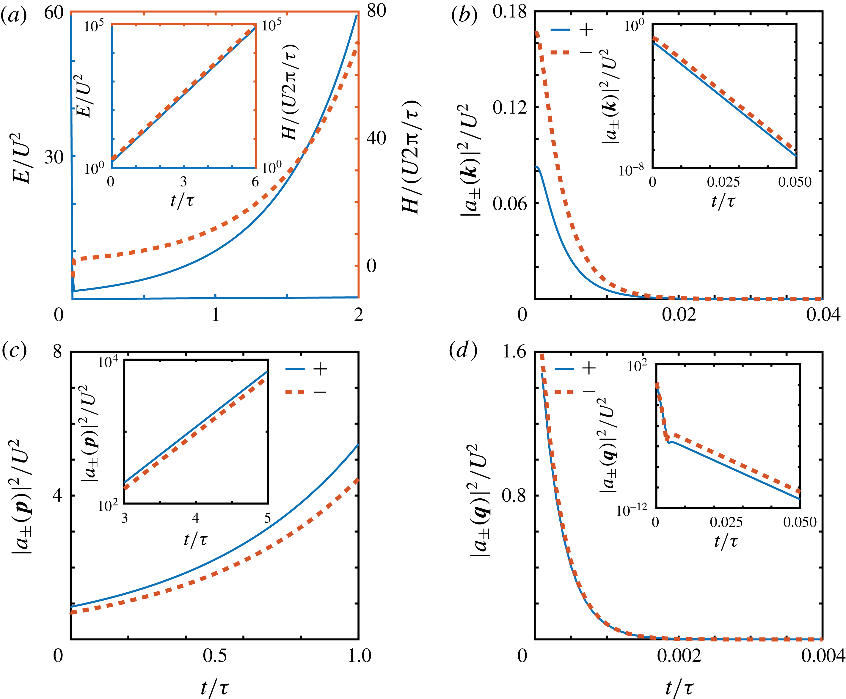
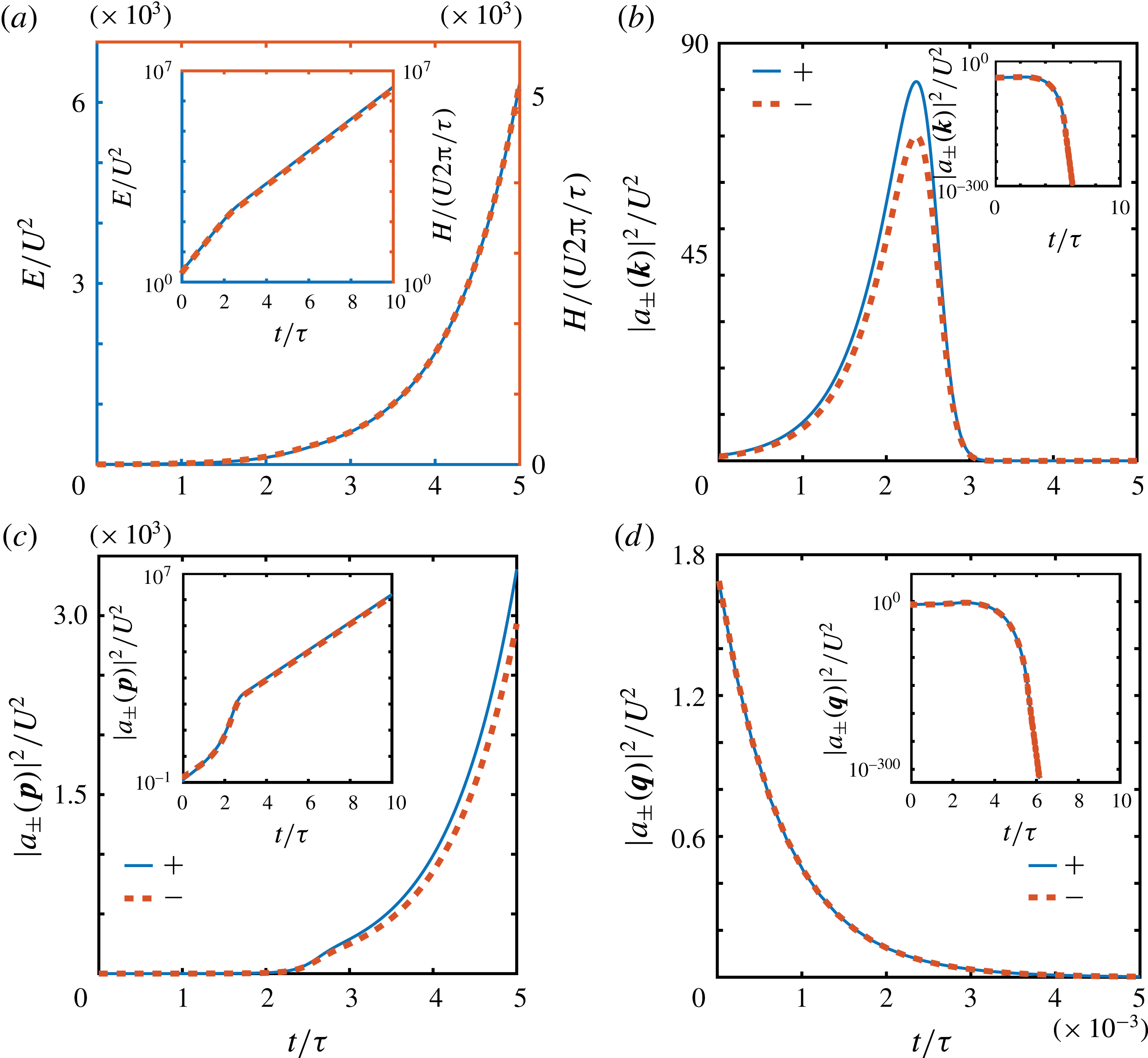
Numerical simulations of (2.3) with polynomial dispersion (1.4) initiated with random complex initial conditions show that active triads (
 $p<k<q$
) are unstable when forced at small wavenumbers
 $p$
. Energy and helicity increase exponentially (a), reflecting the exponential growth of the forced helical mode (c) and overdamped decay of the passive helical modes (b,d). Parameters:
 $\{\boldsymbol{k},\boldsymbol{p},\boldsymbol{q}\}=[(-14,-13,0),(4,-11,0),(10,24,0)]$
, box size
 $L=24\unicode[STIX]{x1D6EC}$
.

The asymptotic growth of the forced modes
 $A_{q}$
and
 $B_{q}$
implies that both energy and helicity increase exponentially, as confirmed in figure 2(a). Thus, at the level of a single triad, the mirror-symmetry breaking may be generated by the following process in the full model (1.3): the rigid body quickly approaches a state in which it is rotating about the
 $q$
-axis, with the angular speed growing exponentially, while the particle accelerates in the direction of
 $q$
or in the direction directly opposite, producing positive or negative helicity, respectively, depending on initial conditions. Spontaneous generation of non-zero helicity thus is a direct consequence of forcing through a linear instability.
A similar description characterised by exponential growth of energy and helicity applies when active triads are forced at the large scale
 $p$
, see figure 3. What distinguishes the two types of forcing is the nature of the damping of the dissipative modes. When forced at large wavenumbers
 $q$
, the decay is underdamped exhibiting oscillations, figure 2(b,c), whereas forcing at the small wavenumbers
 $p$
results in overdamped dynamics, as shown in figure 3(b,d), a direct consequence of the dependence of the damping force on the wavenumber magnitude. The asymptotic response of the system (2.3) when two modes are forced is identical to the above scenarios when one mode is forced, as discussed in the appendix A.
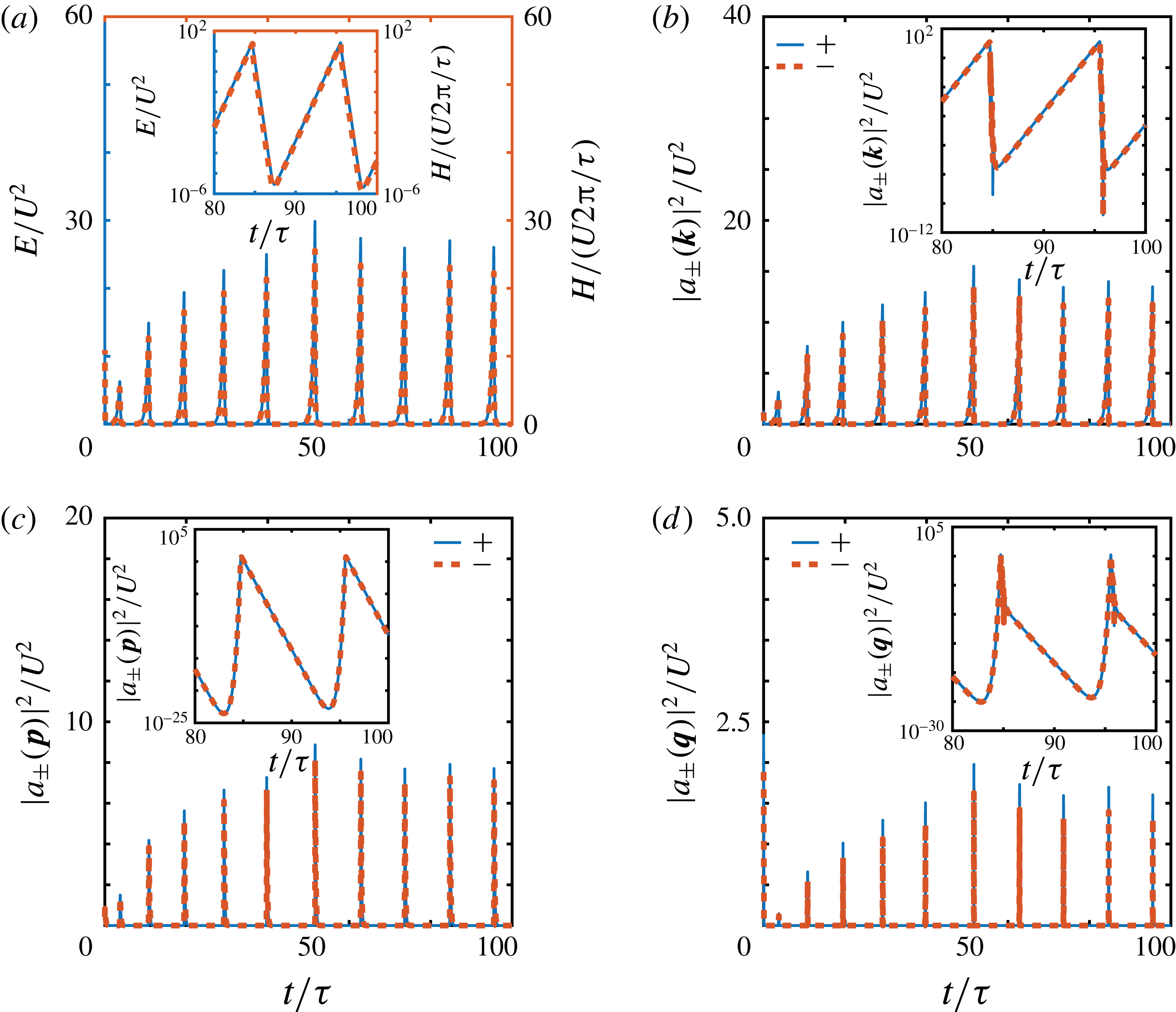
Numerical simulations of (2.3) with polynomial dispersion (1.4) initiated with random complex initial conditions show that active triads (
 $p<k<q$
) are stable when forced at intermediate scales
 $k$
. The energy and helicity (a) as well as the amplitudes of the helical modes (b–d) stay bounded and soon take the form of very rapid charge–discharge bursts, reflecting the collapse of the dynamics onto a limit cycle, see figure 5. Note the different
 $y$
-scales in (b–d), which indicate that the energy produced by the intermediate scale is primarily send to large scales. This is a manifestation of the upward transfer at the level of a single triad. Parameters:
 $\{\boldsymbol{k},\boldsymbol{p},\boldsymbol{q}\}=[(12,1,0),(3,7,0),(-15,-8,0)]$
, box size
 $L=24\unicode[STIX]{x1D6EC}$
.

3.2 Stable triads: rigid body forced at the middle principal axis
For a rigid body forced at the middle principal axis we expect periodic behaviour since the nonlinearity destabilises the action of the linear forcing in this case. Numerical simulations of (2.3) with
 $D_{kk}<0$
but
 $D_{pp}>0$
and
 $D_{qq}>0$
show that the system equilibrates by developing periodic bursts characterised by alternating exponential growth and decay of energy, helicity and the helical modes, suggesting the existence of a stable limit cycle, see figure 4.
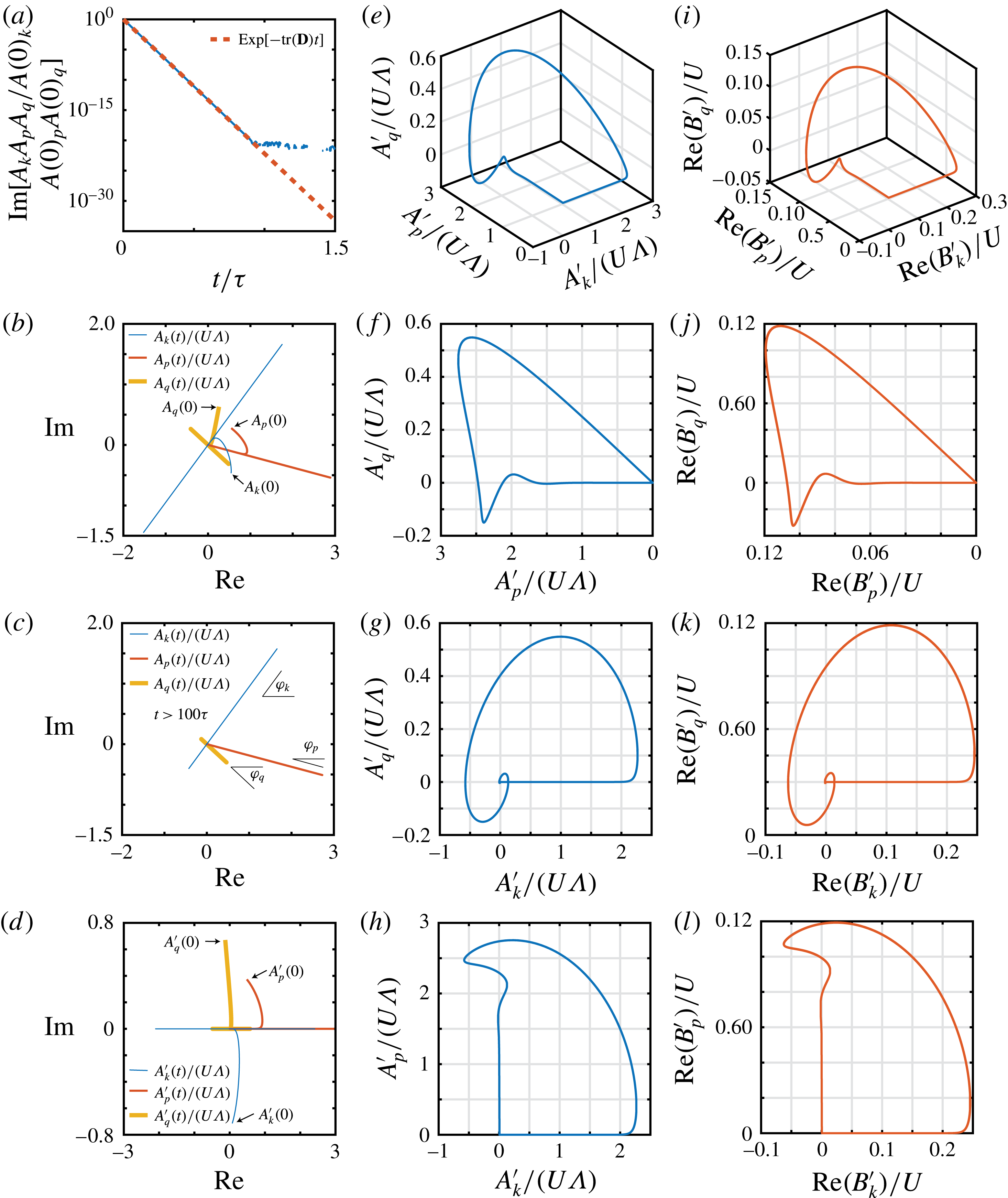
Asymptotic analysis of the results in figure 4: the dynamics of stable active triads eventually collapses onto a limit cycle in a real three-dimensional subspace. (a) The cubic quantity
 $\operatorname{Im}(A_{k}A_{p}A_{q})$
decays in accordance with (2.11) until the machine double-precision limit is reached. (b) Complex trajectories traced out by the modes
 $\boldsymbol{A}(t)=(A_{k}(t),A_{p}(t),A_{q}(t))$
approach straight lines at an exponential rate. (c) Trajectories in (b) for
 $t>100\unicode[STIX]{x1D70F}$
. The lines are characterised by the angles
 $(\unicode[STIX]{x1D719}_{k},\unicode[STIX]{x1D719}_{p},\unicode[STIX]{x1D719}_{q})=(0.759,-0.185,-0.574)$
, such that
 $\unicode[STIX]{x1D719}_{k}+\unicode[STIX]{x1D719}_{p}+\unicode[STIX]{x1D719}_{q}=0$
, as required by vanishing of
 $\operatorname{Im}(A_{k}A_{p}A_{q})$
. (d) The phases define the change of variables
 $(A_{k}^{\prime },A_{p}^{\prime },A_{q}^{\prime })=(\text{e}^{-\text{i}\unicode[STIX]{x1D719}_{k}}A_{k},\text{e}^{-\text{i}\unicode[STIX]{x1D719}_{p}}A_{p},\text{e}^{-\text{i}\unicode[STIX]{x1D719}_{q}}A_{q})$
and
 $(B_{k}^{\prime },B_{p}^{\prime },B_{q}^{\prime })=(\text{e}^{-\text{i}\unicode[STIX]{x1D719}_{k}}B_{k},\text{e}^{-\text{i}\unicode[STIX]{x1D719}_{p}}B_{p},\text{e}^{-\text{i}\unicode[STIX]{x1D719}_{q}}B_{q})$
, which leaves the differential equations (2.3) unchanged, but rotates the complex trajectories so that the variables
 $(A_{k}^{\prime }(t),A_{p}^{\prime }(t),A_{q}^{\prime }(t))$
become real in the limit
 $t\rightarrow \infty$
. (e) In this three-dimensional real subspace,
 $\boldsymbol{A}^{\prime }(t)$
collapses onto a stable limit cycle. (f–h) Projections of the limit cycle of
 $\boldsymbol{A}^{\prime }(t)$
onto the coordinate planes. (i)
 $\boldsymbol{B}^{\prime }(t)$
also develops a limit cycle, shown is the real part. (j–l) The corresponding projections of
 $\operatorname{Re}\boldsymbol{B}^{\prime }(t)$
onto the coordinate planes.

To numerically verify the existence of a limit cycle in the system (2.3a
) initiated with generic complex initial conditions, we now illustrate how to determine the three-dimensional real subspace onto which the system converges. We first note that the numerical solutions obey the property (iii) until the machine precision is reached; see figure 5(a). As a consequence, equation (2.12) implies that each mode either vanishes, stops moving or its trajectory in the complex plane approaches a line through the origin. In the present case of forcing the intermediate wavenumber
 $k$
all three modes follow the last scenario: the complex trajectories
 $(A_{k}(t),A_{p}(t),A_{q}(t))$
become straight lines, see figure 5(b), with well-defined phase angles
 $(\unicode[STIX]{x1D719}_{k},\unicode[STIX]{x1D719}_{p},\unicode[STIX]{x1D719}_{q})$
, that satisfy
 $\unicode[STIX]{x1D719}_{k}+\unicode[STIX]{x1D719}_{p}+\unicode[STIX]{x1D719}_{q}=0$
, see figure 5(c). We use these angles to define the change of variables
 $(A_{k}^{\prime },A_{p}^{\prime },A_{q}^{\prime })=(\text{e}^{-\text{i}\unicode[STIX]{x1D719}_{k}}A_{k},\text{e}^{-\text{i}\unicode[STIX]{x1D719}_{p}}A_{p},\text{e}^{-\text{i}\unicode[STIX]{x1D719}_{q}}A_{q})$
and
 $(B_{k}^{\prime },B_{p}^{\prime },B_{q}^{\prime })=(\text{e}^{-\text{i}\unicode[STIX]{x1D719}_{k}}B_{k},\text{e}^{-\text{i}\unicode[STIX]{x1D719}_{p}}B_{p},\text{e}^{-\text{i}\unicode[STIX]{x1D719}_{q}}B_{q})$
. This change of variables does not affect (2.3), it only rotates the complex trajectories so that the three modes
 $(A_{k}^{\prime },A_{p}^{\prime },A_{q}^{\prime })$
approach a real three-dimensional subspace at an exponential rate, figure 5(d). The asymptotic trajectory in that subspace reveals a limit cycle, figure 5(e–h), as expected from the rigid-body correspondence. The limit cycle represents exponential growth of the rotation rate about the
 $k$
-axis until the nonlinear effects destabilise it, followed by a rapid discharge along the two dissipative axes. The discharge along the
 $q$
-axis represents energy transfer to small scales, while the discharge along the
 $p$
-axis represents energy transfer to large scales. This behaviour likely explains, at the level of individual triadic interactions, the origin of the steady-state upscale energy transfer in the full system (1.3).
3.3 Only stable triads admit a fixed point
We still mention that the triadic system (2.3) forced at the intermediate wavenumber (and only in that case) exhibits a family of fixed points (see appendix B for details)
 $$\begin{eqnarray}\displaystyle \left[\begin{array}{@{}c@{}}A_{k}\\ A_{p}\\ A_{q}\end{array}\right] & = & \displaystyle \sqrt{\unicode[STIX]{x1D6FC}}\left[\begin{array}{@{}c@{}}\sqrt{|p^{2}-q^{2}|/|D_{kk}|}/k\\ \sqrt{|q^{2}-k^{2}|/|D_{pp}|}/p\\ \sqrt{|k^{2}-p^{2}|/|D_{qq}|}/q\end{array}\right],\end{eqnarray}$$
 $$\begin{eqnarray}\displaystyle \left[\begin{array}{@{}c@{}}B_{k}\\ B_{p}\\ B_{q}\end{array}\right] & = & \displaystyle \left[\begin{array}{@{}c@{}}k\sqrt{|p^{2}-q^{2}|/|D_{kk}|}[c_{1}+\text{i}c_{2}(-k^{2}+p^{2}+q^{2})]\\ p\sqrt{|q^{2}-k^{2}|/|D_{pp}|}[c_{1}+\text{i}c_{2}(k^{2}-p^{2}+q^{2})]\\ q\sqrt{|k^{2}-p^{2}|/|D_{qq}|}[c_{1}+\text{i}c_{2}(k^{2}+p^{2}-q^{2})]\end{array}\right],\end{eqnarray}$$
where
 $$\begin{eqnarray}\displaystyle \unicode[STIX]{x1D6FC}=-\det (\unicode[STIX]{x1D644}\unicode[STIX]{x1D63F})/(4\unicode[STIX]{x1D6E5}^{2}|p^{2}-q^{2}||q^{2}-k^{2}||k^{2}-p^{2}|). & & \displaystyle\end{eqnarray}$$
The arbitrary real constants
 $c_{1}$
and
 $c_{2}$
determine energy and helicity. The property (ii) in § 2.2 also implies that we can rotate the solution in the complex plane provided the three phases sum to zero. The fixed points are unstable to linear perturbations.
4 Implications for classical triads
In this section, we classify the geometry of the solutions of (2.3a
) for the case
 $\unicode[STIX]{x1D63F}=\text{0}$
corresponding to the triad truncation of the Euler equations
 $$\begin{eqnarray}\displaystyle \unicode[STIX]{x1D644}\dot{\boldsymbol{A}}=2\unicode[STIX]{x1D6E5}(\unicode[STIX]{x1D644}\boldsymbol{A}^{\ast }\times \boldsymbol{A}^{\ast }). & & \displaystyle\end{eqnarray}$$
The system (4.1) exhibits three constants of motion
 $$\begin{eqnarray}\displaystyle \left.\begin{array}{@{}c@{}}k^{2}|A_{k}|^{2}+p^{2}|A_{p}|^{2}+q^{2}|A_{q}|^{2}=E\\ k^{4}|A_{k}|^{2}+p^{4}|A_{p}|^{2}+q^{4}|A_{q}|^{2}=\unicode[STIX]{x1D6FA}\\ A_{k}A_{p}A_{q}-A_{k}^{\ast }A_{p}^{\ast }A_{q}^{\ast }=C.\end{array}\right\} & & \displaystyle\end{eqnarray}$$
The quadratic constants
 $E$
and
 $\unicode[STIX]{x1D6FA}$
were found by Moffatt (Reference Moffatt2014b
), the new cubic constant
 $C$
was derived in § 2.2 above. The triple (4.2) suggests that the system (4.1) is confined to a three-dimensional surface in a six-dimensional phase space. We next summarise a series of results classifying the solutions to (4.1), which are rigorously proven in appendix C.
In the six-dimensional phase space for the system for
 $\boldsymbol{A}(t)$
, we consider separately the following subsets of
 $\mathbb{R}^{6}$
 $$\begin{eqnarray}\displaystyle Z_{1} & = & \displaystyle \{A_{p}=0,A_{q}=0\}\cup \{A_{q}=0,A_{k}=0\}\cup \{A_{k}=0,A_{p}=0\},\end{eqnarray}$$
 $$\begin{eqnarray}\displaystyle Z_{3} & = & \displaystyle \{|A_{k}||A_{p}||A_{q}|\neq 0,\text{Re}(A_{k}A_{p}A_{q})=0\}\nonumber\\ \displaystyle & & \displaystyle \cap \,\left\{|A_{q}|^{2}|A_{k}|^{2}k^{2}q^{2}(k^{2}-q^{2})+|A_{p}|^{2}|A_{k}|^{2}p^{2}k^{2}(p^{2}-k^{2})\right.\nonumber\\ \displaystyle & & \displaystyle \left.+\,|A_{p}|^{2}|A_{q}|^{2}q^{2}p^{2}(q^{2}-p^{2})=0\right\}.\end{eqnarray}$$
 $Z_{1}$
correspond to fixed points of (4.1). For initial conditions in
 $Z_{3}$
, the system (4.1) is solved exactly by a quasi-periodic motion with constant amplitudes and phases evolving linearly in time according to
 $$\begin{eqnarray}\displaystyle \left.\begin{array}{@{}c@{}}\unicode[STIX]{x1D719}_{k}=\pm [(p^{2}-q^{2})|A_{p}||A_{q}|/(k^{2}|A_{k}|)]t+c_{k}\\ \unicode[STIX]{x1D719}_{p}=\pm [(q^{2}-k^{2})|A_{q}||A_{k}|/(p^{2}|A_{p}|)]t+c_{p}\\ \unicode[STIX]{x1D719}_{q}=\pm [(k^{2}-p^{2})|A_{k}||A_{p}|/(q^{2}|A_{q}|)]t+c_{q},\end{array}\right\} & & \displaystyle\end{eqnarray}$$
where the equalities hold modulo
 $2\unicode[STIX]{x03C0}$
and the constants
 $c_{i}$
are chosen so that
 $\unicode[STIX]{x1D719}_{k}+\unicode[STIX]{x1D719}_{p}+\unicode[STIX]{x1D719}_{q}=\unicode[STIX]{x03C0}/2$
or
 $\unicode[STIX]{x1D719}_{k}+\unicode[STIX]{x1D719}_{p}+\unicode[STIX]{x1D719}_{q}=3/2\unicode[STIX]{x03C0}$
holds, as required by the definition of
 $Z_{3}$
. Importantly, for initial conditions in
 $Z_{3}$
the sum of phases is conserved, so the system (4.1) stays in
 $Z_{3}$
and the phase space in fact can be reduced to a torus
 $\mathbb{T}^{2}$
. A typical trajectory for initial conditions on
 $Z_{3}$
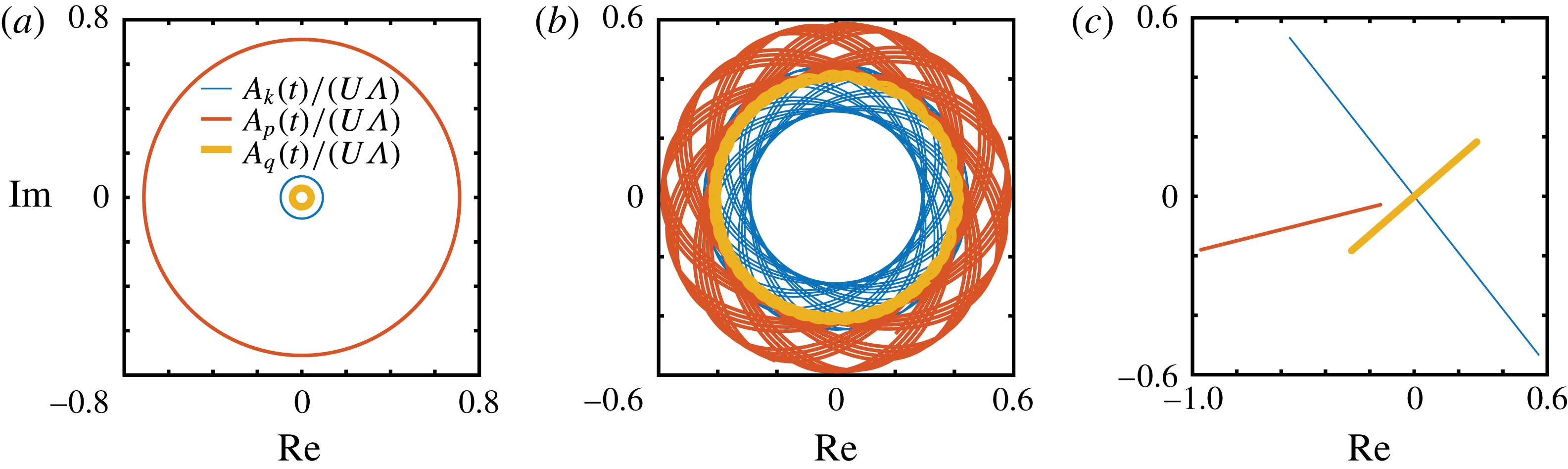
is shown in figure 6(a). In summary, fixed points and quasi-periodic motion completely characterise the solutions of (4.1) for initial conditions in
 $Z_{1}$
and
 $Z_{3}$
, respectively.
Types of orbits
 $\boldsymbol{A}(t)$
in the complex plane for the classical system (2.3a
) with
 $\unicode[STIX]{x1D63F}=\text{0}$
include: fixed points (not shown), circular orbits for initial conditions in the set
 $Z_{3}$
(a), orbits resulting from trajectories on a three-torus for generic initial conditions (b), straight lines for initial conditions with
 $C=0$
in (4.2), in which case the system reduces to the classical Euler equations for a rigid body (c).

We now consider the most important generic case of initial conditions in the complement
 $N=\mathbb{R}^{6}\backslash (Z_{1}\cap Z_{3})$
. In
 $N$
, the differential of (4.2) has full rank, implying that (4.2) defines a three-dimensional manifold in
 $N$
, that is, the solutions of (4.1) are confined to a smooth three-dimensional surface. For generic values of the triple
 $(E,\unicode[STIX]{x1D6FA},C)$
, this surface is in fact a three-torus
 $\mathbb{T}^{3}$
(or several copies of such tori). A typical trajectory in such a generic case is shown in figure 6(b). There are also special cases of
 $(E,\unicode[STIX]{x1D6FA},C)$
for which the manifold looks like (copies of) a product of a line and a torus
 $\mathbb{R}\times \mathbb{T}^{2}$
and/or (copies of)
 $\mathbb{T}^{3}$
. The reader is referred to appendix C for more details and rigorous proofs.
Finally, we still note that, since the solutions
 $\boldsymbol{A}(t)$
remain continuous and bounded for all
 $t$
, the linear system for
 $\boldsymbol{B}(t)$
can be solved exactly, at least formally, in terms of time-ordered matrix exponentials (Gantmacher Reference Gantmacher2000). In the future, it would be interesting to explore in detail potential relations between the above results and recent studies of turbulence in two-dimensional three-component flows (Biferale et al.
Reference Biferale, Buzzicotti and Linkmann2017).
5 Gaussian active turbulence model
The behaviour of individual active triads suggests that the mirror-symmetry breaking and upward energy transfer observed in the GNS system (1.3) are first triggered by unstable active triads and then sustained by stable active triads. Moreover, these effects likely hold for a broader class of forcing schemes provided the dispersion relation
 $\unicode[STIX]{x1D709}(k)$
in (1.3) introduces a narrow band of unstable modes. To test this hypothesis, we numerically study an alternative GNS model where the dispersion relation has the form
 $$\begin{eqnarray}\displaystyle \unicode[STIX]{x1D709}(k)=\unicode[STIX]{x1D6E4}_{0}k^{2}-\unicode[STIX]{x1D6FC}\exp [-(k-k_{0})^{2}/(2\unicode[STIX]{x1D70E}^{2})]. & & \displaystyle\end{eqnarray}$$
The main difference between (5.1) and the polynomial model (1.1) is that the Gaussian activity model (5.1) behaves like a Newtonian fluid with viscosity
 $\unicode[STIX]{x1D6E4}_{0}$
at both large and small scales, see figure 1(a). Equation (5.1) leads to an integro-partial differential equation in position space. In our simulations, we always fix
 $\unicode[STIX]{x1D6E4}_{0}=10^{-6}~\text{m}^{2}~\text{s}^{-1}$
, corresponding to the kinematic viscosity of water. To relate the parameters
 $(\unicode[STIX]{x1D6FC},k_{0},\unicode[STIX]{x1D70E})$
to the characteristic triple
 $(\unicode[STIX]{x1D6EC},\unicode[STIX]{x1D70F},\unicode[STIX]{x1D705})$
, we must solve
 $$\begin{eqnarray}\displaystyle \unicode[STIX]{x1D709}^{\prime }(k_{\unicode[STIX]{x1D6EC}})=0,\quad \unicode[STIX]{x1D70F}=-\unicode[STIX]{x1D709}^{-1}(k_{\unicode[STIX]{x1D6EC}}),\quad \unicode[STIX]{x1D709}(k_{\pm })=0,\quad \unicode[STIX]{x1D705}=k_{+}-k_{-}, & & \displaystyle\end{eqnarray}$$
where
 $k_{\unicode[STIX]{x1D6EC}}=\unicode[STIX]{x03C0}/\unicode[STIX]{x1D6EC}$
is the most unstable wavenumber and
 $k_{\pm }$
are the non-trivial zeros of the dispersion relation
 $\unicode[STIX]{x1D709}(k)$
. Since no closed-form solutions exist, we solve the system (5.2) numerically. We set
 $(\unicode[STIX]{x1D6FC},k_{0},\unicode[STIX]{x1D70E})=(2.544165~\text{ms}^{-1},52.36~\text{mm}^{-1},10~\text{mm}^{-1})$
, yielding
 $(\unicode[STIX]{x1D6EC},\unicode[STIX]{x1D70F},\unicode[STIX]{x1D705})=(65.14~\unicode[STIX]{x03BC}\text{m},0.1~\text{s},1.94~\text{mm}^{-1})$
, which is in the range of typical bacterial suspension values (Słomka & Dunkel Reference Słomka and Dunkel2017b
). Non-dimensionalising according to
 $$\begin{eqnarray}\displaystyle x=\frac{L}{2\unicode[STIX]{x03C0}}\tilde{x},\quad t=T\tilde{t},\quad v=\frac{L/(2\unicode[STIX]{x03C0})}{T}\tilde{v},\quad k=\frac{2\unicode[STIX]{x03C0}}{L}\tilde{k}, & & \displaystyle\end{eqnarray}$$
gives, after dropping the tildes and setting
 $T=(L/2\unicode[STIX]{x03C0})^{2}/\unicode[STIX]{x1D6E4}_{0}$
,
 $$\begin{eqnarray}\displaystyle \unicode[STIX]{x1D709}(k)=k^{2}-T\unicode[STIX]{x1D6FC}\exp \{-[(2\unicode[STIX]{x03C0}/L)k-k_{0}]^{2}/(2\unicode[STIX]{x1D70E}^{2})\}. & & \displaystyle\end{eqnarray}$$
We simulate the dimensionless system in the vorticity-vector potential formulation as described in (Słomka & Dunkel Reference Słomka and Dunkel2017b
) using the Fourier pseudo-spectral method with the ‘
 $3/2$
’-rule (Canuto et al.
Reference Canuto, Hussaini, Quarteroni and Zang1988), discretisation size
 $N=243^{3}$
and time step
 $\text{d}t=5\times 10^{-4}\unicode[STIX]{x1D70F}/T$
. We set the domain size
 $L=42\unicode[STIX]{x1D6EC}$
, which corresponds to the most unstable wavenumber at
 $k_{\unicode[STIX]{x1D6EC}}=21$
. For time stepping, we use a third-order semi-implicit backward differentiation scheme (Ascher, Ruuth & Wetton Reference Ascher, Ruuth and Wetton1995). For this choice of parameters, the resulting flow patterns arise from the balance between the active and passive stresses mediated by the nonlinear advection. Hence, advection and stresses are equally important, suggesting an effective Reynolds number of the order of unity. Indeed, adopting the standard definition of the integral-scale Reynolds number
 $Re$
(Frisch Reference Frisch2004), we find that
 $Re\sim 4.7$
for the simulations in figure 7.
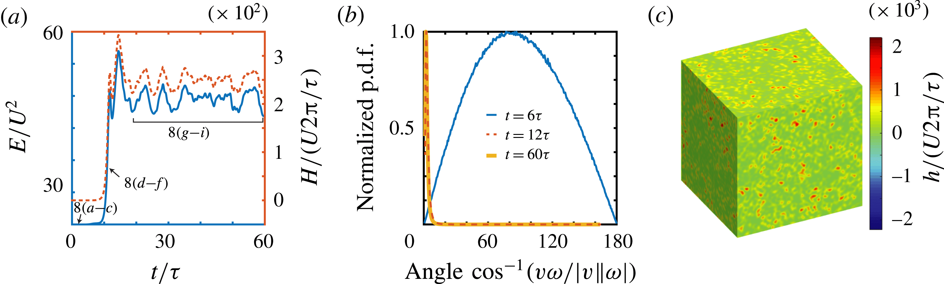
Simulation results for the Gaussian model (5.1). (a) Energy and helicity time series show the initial relaxation phase and the subsequent statistically stationary stage. Time instants and interval labels refer to figure 8. (b) Normalised histograms of the angles between velocity
 $\boldsymbol{v}$
and vorticity
 $\unicode[STIX]{x1D74E}$
at three different time instants confirm that mirror-symmetry breaking is achieved by developing Beltrami-type flows, where velocity and vorticity are nearly aligned. (c) Snapshot of the helicity density field at
 $t=60\unicode[STIX]{x1D70F}$
showing spontaneous symmetry breaking towards positive values.

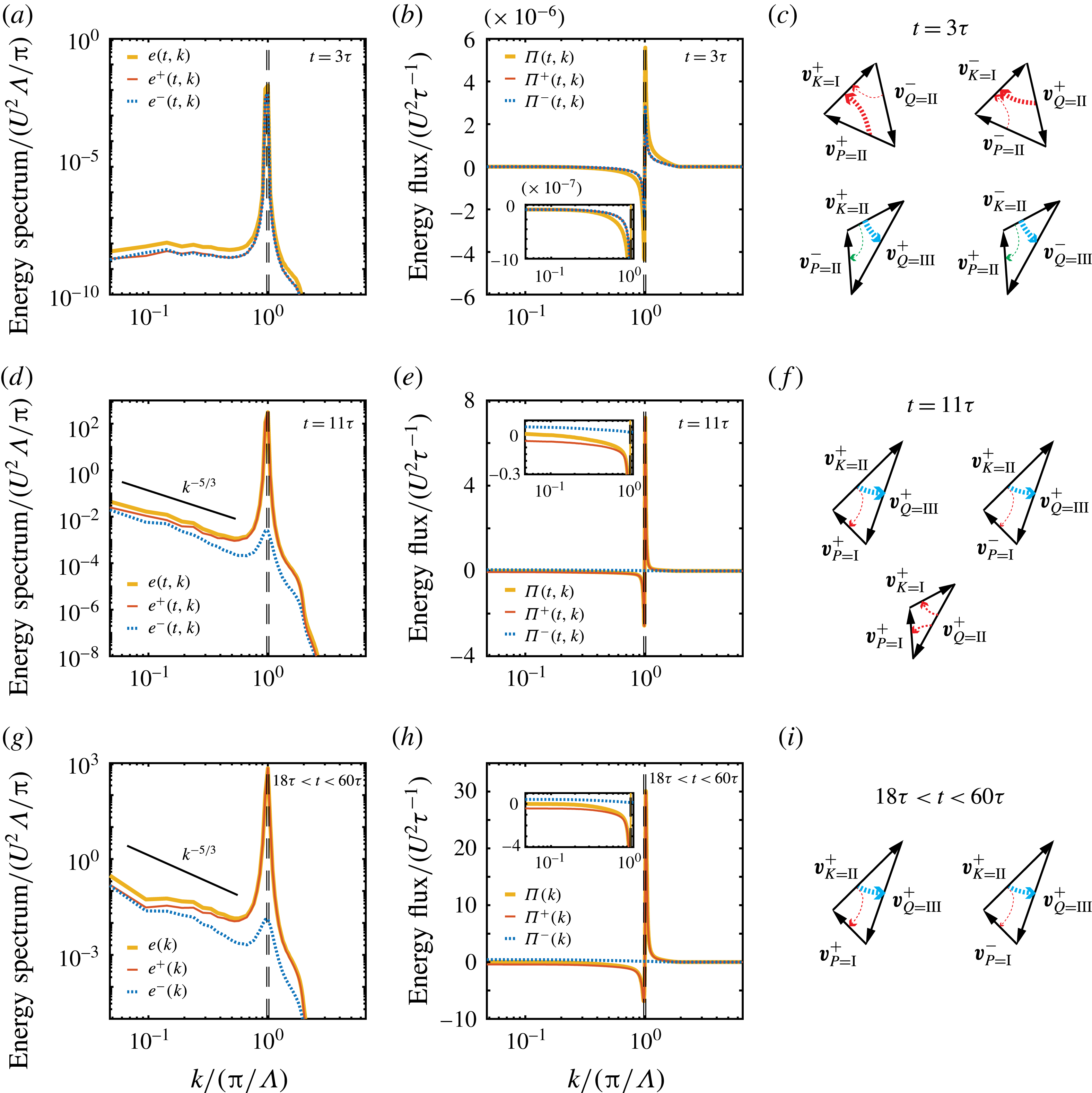
Numerical results for the Gaussian activity model (5.1) based on the simulation in figure 7. Instantaneous (a–f) and average (g–i) energy spectra, fluxes and dominant integrated triads for time instants and intervals indicated in figure 7(a). Vertical dashed lines mark the energy injection range.

To discuss the results of numerical simulations, we use the helical decomposition (Constantin & Majda Reference Constantin and Majda1988; Waleffe Reference Waleffe1992) to expand the velocity field in an orthogonal basis of curl operator eigenvectors
 $\boldsymbol{h}^{\pm }$
 $$\begin{eqnarray}\displaystyle \boldsymbol{v}(t,\boldsymbol{k})=u^{+}(t,\boldsymbol{k})\,\boldsymbol{h}^{+}(\boldsymbol{k})+u^{-}(t,\boldsymbol{k})\,\boldsymbol{h}^{-}(\boldsymbol{k}), & & \displaystyle\end{eqnarray}$$
where
 $\boldsymbol{h}^{\pm }$
satisfy
 $\text{i}\boldsymbol{k}\times \boldsymbol{h}^{\pm }=\pm k\boldsymbol{h}^{\pm }$
with
 $k=|\boldsymbol{k}|$
. The decomposition (5.5) yields a splitting into cumulative energy and flux contributions
 $e^{\pm }(k)$
and
 $\unicode[STIX]{x1D6F1}^{\pm }(k)$
from helical modes
 $u^{\pm }(\boldsymbol{k})$
lying on the wavenumber shell
 $k$
. Specifically,
 $\unicode[STIX]{x1D6F1}^{+}(k)=\sum _{i=1}^{4}\unicode[STIX]{x1D6F1}^{i}(k)$
and
 $\unicode[STIX]{x1D6F1}^{-}(k)=\sum _{i=5}^{8}\unicode[STIX]{x1D6F1}^{i}(k)$
, where
 $\unicode[STIX]{x1D6F1}^{i}(k)$
is one of the eight types of helicity-resolved fluxes and the summation follows the binary ordering of Waleffe (Reference Waleffe1992). To analyse which triads are spontaneously activated at various time instants, we consider combinations
 $K,P,Q\in \{\text{I},\text{II},\text{III}\}$
of the three spectral domains in figure 1(b), with region I corresponding to large scales, II to the energy injection range and III to small scales, and distinguish modes by their helicity index
 $s_{K},s_{P},s_{Q}\in \{\pm \}$
. The helicity-resolved integrated energy flow into the region
 $(K,s_{K})$
due to interaction with regions
 $(P,s_{P})$
and
 $(Q,s_{Q})$
is given by
 $$\begin{eqnarray}\displaystyle \unicode[STIX]{x1D61B}_{KPQ}^{s_{K}s_{P}s_{Q}}={\textstyle \frac{1}{2}}(\tilde{\unicode[STIX]{x1D61B}}_{KPQ}^{s_{K}s_{P}s_{Q}}+\tilde{\unicode[STIX]{x1D61B}}_{KQP}^{s_{K}s_{Q}s_{P}}), & & \displaystyle\end{eqnarray}$$
where the unsymmetrised flows are defined by
 $$\begin{eqnarray}\displaystyle \tilde{\unicode[STIX]{x1D61B}}_{KPQ}^{s_{K}s_{P}s_{Q}}=-\int \text{d}^{3}x\,\boldsymbol{v}_{K}^{s_{K}}\boldsymbol{\cdot }[(\boldsymbol{v}_{P}^{s_{P}}\boldsymbol{\cdot }\unicode[STIX]{x1D735})\boldsymbol{v}_{Q}^{s_{Q}}], & & \displaystyle\end{eqnarray}$$
with
 $\boldsymbol{v}_{K}^{s_{K}}(t,\boldsymbol{x})$
denoting the helical Littlewood–Paley velocity components, obtained by projecting on modes of a given helicity index
 $s_{K}\in \{\pm \}$
restricted to the Fourier space domain
 $K$
. Entries of the tensor
 $\unicode[STIX]{x1D64F}$
are large when the corresponding triads are dominant. For example, a positive (negative) value of
 $\unicode[STIX]{x1D61B}_{I,II,III}^{+++}$
indicates that energy flows into (out of) large scale (I) positive helicity modes due to interactions of these modes with positive helical modes corresponding to energy injection range (II) and small scales (III).
Our numerical simulations show that the Gaussian forcing model (5.1) and the polynomial model (1.4) exhibit qualitatively similar behaviour, cf. figures 7, 8 and corresponding plots in Słomka & Dunkel (Reference Słomka and Dunkel2017b
). The Gaussian activity model also undergoes mirror-symmetry breaking and spontaneously develops a non-zero net helicity, by realising chaotic Beltrami-type flow states in which velocity
 $\boldsymbol{v}$
and vorticity
 $\unicode[STIX]{x1D74E}$
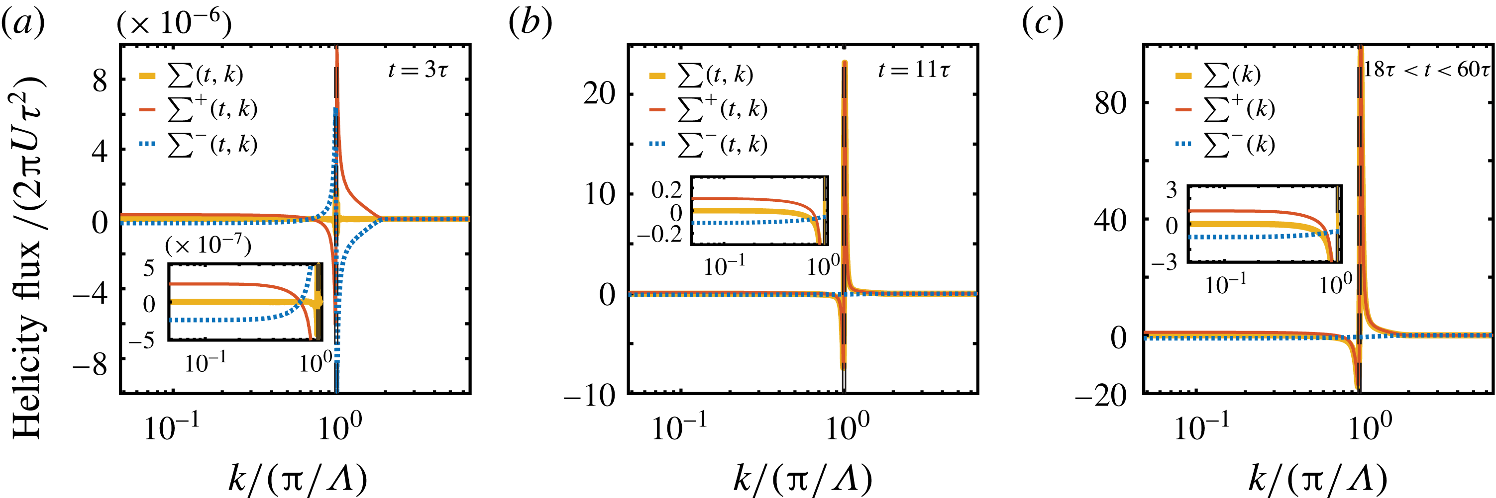
are almost aligned, see figure 7. Figure 8 shows instantaneous and time-averaged energy spectra, energy fluxes and the dominant entries of the integrated triadic energy flows (5.6) for the time instants and intervals marked in figure 7(a). The energy spectra in figures 8(a,d,g) indicate that the system spontaneously selects positive helicity modes at all relevant wavenumbers in this particular realisation, while the energy fluxes in figures 8(b,e,h) are always negative at scales larger than the energy injection range (vertical dashed lines), demonstrating the inverse energy cascade. The corresponding helicity fluxes are shown in figure 11 of the appendix. Similarly to the polynomial case, the upward energy transfer in the Gaussian model is not inertial, as indicated by the wavenumber dependence of the energy fluxes. In particular, it is not necessary to introduce hyper-viscosity at large scales to arrest the upward transfer, and the instantaneous and averaged energy fluxes can be computed directly from the balance between the nonlinear and dissipative and active terms according to equations (S23) and (S33) in Słomka & Dunkel (Reference Słomka and Dunkel2017b
). Unlike the polynomial model, however, the long-time spectra of the Gaussian model develop an approximate Kolmogorov
 $-5/3$
scaling at large wavelengths, see figure 8(d). We attribute this effect to the weak dependence of the energy flux on the wavenumber. More importantly, the dominant integrated energy flows shown in figure 8(c,f,i), where broken arrows indicate the direction of the inter-scale energy transfer and their thickness the relative magnitude of the transfer, are in agreement with the hypothesis that unstable triads drive the initial relaxation until stable triads become dominant and sustain the statistically stationary chaotic flow states.
6 Conclusions
We derived a previously unknown cubic invariant for the triad dynamics and used it to analyse and compare the triad truncations of two generalised Navier–Stokes (GNS) models and the classical Euler equations. In the GNS case, we focused on active triads with one or two modes in the energy injection range and found that their dynamics is asymptotically equivalent to a coupled system consisting of a forced rigid body and a forced particle in a magnetic field. This analogy allows one to distinguish unstable and stable active triads, based on whether the rigid body is forced along the small/large principal axes (large/small scales) or the middle principal axis (intermediate scales), respectively. The dynamics of the active GNS triads differs strongly from those of the classical Euler triads, for which the rigid-body analogy does not hold in general and solutions are confined to a three-torus for generic initial conditions (§ 4).
The existence of unstable and stable triads explains recent numerical results in Słomka & Dunkel (Reference Słomka and Dunkel2017b
), which suggested that the polynomial 3-D GNS models can spontaneously break mirror symmetry by developing Beltrami-like flow states and upward energy transfer: unstable triads induce exponential helicity growth from small perturbations and dominate the initial relaxation. Because of the nonlinear coupling between the triads, the stable triads eventually become dominant and the system settles into a statistically stationary chaotic flow state. In the stationary regime, energy is transferred from the spectral injection range to both large and small scales. This is consistent with the behaviour of stable triads, which develop a limit cycle. In the rigid-body analogy, this limit cycle represents a periodic two-phase process. During the first phase, the rigid body accumulates energy by increasing its spinning rate along the middle principal axis; during the second phase, the accumulated energy is released along the small and large principal axes. This release of the energy corresponds to energy transfer to large and small scales in the untruncated hydrodynamic equations. We confirmed the above picture for an alternative GNS model (5.1), which combines viscous dissipation and active Gaussian forcing, by computing the integrated energy flow between the three spectral domains (large scales, energy injection range and small scales). Unlike the previously studied polynomial model, the Gaussian active turbulence model develops energy spectra that approximately follow Kolmogorov’s
 $-5/3$
scaling at large wavelengths, which may be desirable in applications to microbial suspensions.
More broadly, the above results suggest that parity violation and an inverse energy cascade may be generic features of turbulence models where the forcing term depends on the velocity field. The degree to which the mirror symmetry is broken or the proportion of energy that is transferred to small and large scales should depend on the particular forcing considered. The two GNS models (1.4) and (5.1) analysed here are basic examples that introduce a bandwidth of linearly unstable modes. These models can help guide theoretical efforts to find other forcing schemes that realise specific desired features, such as the magnitude of the upward transfer or its inertial character. Biological and engineered active fluids are promising candidates for the experimental implementation, as GNS models can be fitted to reproduce experimentally observed velocity correlation functions (Słomka & Dunkel Reference Słomka and Dunkel2017b ). However, the general nature of the triad-based arguments presented here suggests that other non-equilibrium fluids might also be capable of breaking mirror symmetry and developing upward energy transfer. Last but not least, our results indicate that helical flows (Moffatt Reference Moffatt2014a ) and the Beltrami-type flows in particular, which have been primarily studied as exact stationary solutions of the Euler equations (Arnold & Khesin Reference Arnold and Khesin1999) and in the context of magnetodynamics (Marsh Reference Marsh1996; Yoshida et al. Reference Yoshida, Mahajan, Ohsaki, Iqbal and Shatashvili2001; Hudson, Hole & Dewar Reference Hudson, Hole and Dewar2007), could be more ubiquitous than previously thought.
Acknowledgements
The authors thank R. Rosales, L. Faria and V. Heinonen for helpful discussions. This work was supported by an Alfred P. Sloan Research Fellowship (J.D.), an Edmund F. Kelly Research Award (J.D.) and a Complex Systems Scholar Award of the James S. McDonnell Foundation (J.D.).
Appendix A. Triads forced at two legs
Figures 9 and 10 show the results of numerical simulations of the system (2.3) when it is forced at intermediate and small scales (figure 9) and at large and intermediate scales (figure 10). In both cases, even though the intermediate scale is forced, it is eventually suppressed and the asymptotic behaviour becomes identical to the single-mode forcing case, as described in § 3.1.
Numerical simulations of the triad dynamics (2.3) initiated with generic complex initial conditions show that active triads (
 $p<k<q$
) are unstable when forced at intermediate
 $k$
and small
 $q$
scales. Energy and helicity increase exponentially (a), reflecting the exponential growth of one of the forced modes (d) and underdamped decay of the remaining forced mode (b) and the passive mode (c). Parameters:
 $\{\boldsymbol{k},\boldsymbol{p},\boldsymbol{q}\}=[(4,-11,0),(-9,-1,0),(5,12,0)]$
, box size
 $L=24\unicode[STIX]{x1D6EC}$
.

Numerical simulations of the triad dynamics (2.3) initiated with generic complex initial conditions show that active triads (
 $p<k<q$
) are unstable when forced at large
 $p$
and intermediate
 $k$
scales. Energy and helicity increase exponentially (a), reflecting the exponential growth of one of the forced modes (c) and overdamped decay of the remaining forced mode (b) and the passive mode (d). Parameters:
 $\{\boldsymbol{k},\boldsymbol{p},\boldsymbol{q}\}=[(5,11,0),(8,8,0),(-13,-19,0)]$
, box size
 $L=24\unicode[STIX]{x1D6EC}$
.

Appendix B. Fixed points of the active triadic system and their linear stability
We show that the triadic system (2.3) forced at the intermediate wavenumber exhibits a linearly unstable fixed point. To this end, we first look for time-independent solutions of (2.3a ), satisfying
 $$\begin{eqnarray}\displaystyle \unicode[STIX]{x1D63F}\unicode[STIX]{x1D644}\boldsymbol{A}=2\unicode[STIX]{x1D6E5}(\unicode[STIX]{x1D644}\boldsymbol{A}^{\ast }\times \boldsymbol{A}^{\ast }). & & \displaystyle\end{eqnarray}$$
Remembering the convention
 $p<k<q$
and using the polar representation
 $A_{k}=|A_{k}|\text{e}^{\text{i}\unicode[STIX]{x1D719}_{k}}$
we demand that
 $$\begin{eqnarray}\displaystyle -s_{k}|D_{kk}|k^{2}|A_{k}|\text{e}^{\text{i}\unicode[STIX]{x1D719}} & = & \displaystyle 2\unicode[STIX]{x1D6E5}|p^{2}-q^{2}||A_{p}||A_{q}|,\end{eqnarray}$$
 $$\begin{eqnarray}\displaystyle s_{p}|D_{pp}|p^{2}|A_{p}|\text{e}^{\text{i}\unicode[STIX]{x1D719}} & = & \displaystyle 2\unicode[STIX]{x1D6E5}|q^{2}-k^{2}||A_{q}||A_{k}|,\end{eqnarray}$$
 $$\begin{eqnarray}\displaystyle s_{q}|D_{qq}|q^{2}|A_{q}|\text{e}^{\text{i}\unicode[STIX]{x1D719}} & = & \displaystyle 2\unicode[STIX]{x1D6E5}|k^{2}-p^{2}||A_{k}||A_{p}|,\end{eqnarray}$$
where
 $s_{k}=1$
if
 $D_{kk}>0$
and
 $s_{k}=-1$
if
 $D_{kk}<0$
and
 $\unicode[STIX]{x1D719}=\unicode[STIX]{x1D719}_{k}+\unicode[STIX]{x1D719}_{p}+\unicode[STIX]{x1D719}_{q}$
. Matching the phases, requires that
 $$\begin{eqnarray}\displaystyle \unicode[STIX]{x1D719}+\unicode[STIX]{x1D719}_{-s_{k}}=\unicode[STIX]{x1D719}+\unicode[STIX]{x1D719}_{s_{p}}=\unicode[STIX]{x1D719}+\unicode[STIX]{x1D719}_{s_{q}}=0, & & \displaystyle\end{eqnarray}$$
where the equalities hold modulo
 $2\unicode[STIX]{x03C0}$
. The only way to satisfy the above restrictions is to choose
 $s_{k}=-1$
and
 $s_{p}=s_{q}=1$
, that is, a fixed point can exist only when the intermediate wavenumber is forced. Of course, we must then have
 $\unicode[STIX]{x1D719}=0$
, which leaves a two-parameter family of fixed points. Without loss of generality, we can set all phases to zero
 $\unicode[STIX]{x1D719}_{k}=\unicode[STIX]{x1D719}_{p}=\unicode[STIX]{x1D719}_{q}=0$
. Matching the amplitudes gives
 $$\begin{eqnarray}\displaystyle |D_{kk}|k^{2}|A_{k}| & = & \displaystyle 2\unicode[STIX]{x1D6E5}|p^{2}-q^{2}||A_{p}||A_{q}|,\end{eqnarray}$$
 $$\begin{eqnarray}\displaystyle |D_{pp}|p^{2}|A_{p}| & = & \displaystyle 2\unicode[STIX]{x1D6E5}|q^{2}-k^{2}||A_{q}||A_{k}|,\end{eqnarray}$$
 $$\begin{eqnarray}\displaystyle |D_{qq}|q^{2}|A_{q}| & = & \displaystyle 2\unicode[STIX]{x1D6E5}|k^{2}-p^{2}||A_{k}||A_{p}|.\end{eqnarray}$$
Furthermore, we still have the following two identities
 $$\begin{eqnarray}\displaystyle -|D_{kk}|k^{2}|A_{k}|^{2}+|D_{pp}|p^{2}|A_{p}|^{2}+|D_{qq}|q^{2}|A_{q}|^{2} & = & \displaystyle 0,\end{eqnarray}$$
 $$\begin{eqnarray}\displaystyle -|D_{kk}|k^{4}|A_{k}|^{2}+|D_{pp}|p^{4}|A_{p}|^{2}+|D_{qq}|q^{4}|A_{q}|^{2} & = & \displaystyle 0,\end{eqnarray}$$
which represent energy and in-plane enstrophy balance: energy and enstrophy produced at the wavenumber
 $k$
are dissipated at wavenumbers
 $p$
and
 $q$
. The two constraints leave one degree of freedom represented by the line
 $$\begin{eqnarray}\displaystyle \left[\begin{array}{@{}c@{}}|A_{k}|^{2}\\ |A_{p}|^{2}\\ |A_{q}|^{2}\end{array}\right]=\unicode[STIX]{x1D6FC}\left[\begin{array}{@{}c@{}}\displaystyle \frac{|p^{2}-q^{2}|}{|D_{kk}|k^{2}}\\ \displaystyle \frac{|q^{2}-k^{2}|}{|D_{pp}|p^{2}}\\ \displaystyle \frac{|k^{2}-p^{2}|}{|D_{qq}|q^{2}}\end{array}\right]. & & \displaystyle\end{eqnarray}$$
The positive constant
 $\unicode[STIX]{x1D6FC}$
is fixed by inserting the above expression into (B 6), which then yields for
 $\boldsymbol{A}$
the fixed point
 $$\begin{eqnarray}\displaystyle \left[\begin{array}{@{}c@{}}A_{k}\\ A_{p}\\ A_{q}\end{array}\right]=\unicode[STIX]{x1D6FC}^{1/2}\left[\begin{array}{@{}c@{}}\displaystyle \sqrt{\frac{|p^{2}-q^{2}|}{|D_{kk}|k^{2}}}\\ \displaystyle \sqrt{\frac{|q^{2}-k^{2}|}{|D_{pp}|p^{2}}}\\ \displaystyle \sqrt{\frac{|k^{2}-p^{2}|}{|D_{qq}|q^{2}}}\end{array}\right], & & \displaystyle\end{eqnarray}$$
where
 $$\begin{eqnarray}\displaystyle \unicode[STIX]{x1D6FC}=-\det (\unicode[STIX]{x1D644}\unicode[STIX]{x1D63F})/(4\unicode[STIX]{x1D6E5}^{2}|p^{2}-q^{2}||q^{2}-k^{2}||k^{2}-p^{2}|). & & \displaystyle\end{eqnarray}$$
All other fixed points are obtained by the transformation
 $$\begin{eqnarray}\displaystyle \left[\begin{array}{@{}c@{}}A_{k}\\ A_{p}\\ A_{q}\end{array}\right]\rightarrow \left[\begin{array}{@{}c@{}}A_{k}\text{e}^{\text{i}\unicode[STIX]{x1D719}_{k}}\\ A_{p}\text{e}^{\text{i}\unicode[STIX]{x1D719}_{p}}\\ A_{q}\text{e}^{\text{i}\unicode[STIX]{x1D719}_{q}}\end{array}\right], & & \displaystyle\end{eqnarray}$$
where
 $\unicode[STIX]{x1D719}_{k}+\unicode[STIX]{x1D719}_{p}+\unicode[STIX]{x1D719}_{q}=0$
.
We now turn to the fixed points of the system for
 $\boldsymbol{B}(t)=\operatorname{Re}\boldsymbol{B}(t)+\text{i}\operatorname{Im}\boldsymbol{B}(t)$
, that is, we look for time-independent solutions of (2.3b
) with
 $\boldsymbol{A}$
given by (B 12). In this case, the system decouples into two linear equations for the real and imaginary parts
 $$\begin{eqnarray}\displaystyle \unicode[STIX]{x1D63F}\operatorname{Re}\boldsymbol{B} & = & \displaystyle 2\unicode[STIX]{x1D6E5}\operatorname{Re}\boldsymbol{B}\times \boldsymbol{A},\end{eqnarray}$$
 $$\begin{eqnarray}\displaystyle \unicode[STIX]{x1D63F}\operatorname{Im}\boldsymbol{B} & = & \displaystyle -2\unicode[STIX]{x1D6E5}\operatorname{Im}\boldsymbol{B}\times \boldsymbol{A}.\end{eqnarray}$$
In both cases the null-space is one-dimensional, generated by the vectors
 $$\begin{eqnarray}\displaystyle \left[\begin{array}{@{}c@{}}\operatorname{Re}B_{k}\\ \operatorname{Re}B_{p}\\ \operatorname{Re}B_{q}\end{array}\right]=\left[\begin{array}{@{}c@{}}\displaystyle k\sqrt{\frac{|p^{2}-q^{2}|}{|D_{kk}|}}\\ \displaystyle p\sqrt{\frac{|q^{2}-k^{2}|}{|D_{pp}|}}\\ \displaystyle q\sqrt{\frac{|k^{2}-p^{2}|}{|D_{qq}|}}\end{array}\right],\quad \left[\begin{array}{@{}c@{}}\operatorname{Im}B_{k}\\ \operatorname{Im}B_{p}\\ \operatorname{Im}B_{q}\end{array}\right]=\left[\begin{array}{@{}c@{}}\displaystyle k\sqrt{\frac{|p^{2}-q^{2}|}{|D_{kk}|}}(-k^{2}+p^{2}+q^{2})\\ \displaystyle p\sqrt{\frac{|q^{2}-k^{2}|}{|D_{pp}|}}(k^{2}-p^{2}+q^{2})\\ \displaystyle q\sqrt{\frac{|k^{2}-p^{2}|}{|D_{qq}|}}(k^{2}+p^{2}-q^{2})\end{array}\right]. & & \displaystyle\end{eqnarray}$$
The fixed point for
 $\boldsymbol{B}$
is obtained by combining the real and imaginary parts,
 $$\begin{eqnarray}\displaystyle \left[\begin{array}{@{}c@{}}B_{k}\\ B_{p}\\ B_{q}\end{array}\right] & \unicode[STIX]{x1D6FC}^{1/2}\left[\begin{array}{@{}c@{}}\displaystyle k\sqrt{\frac{|p^{2}-q^{2}|}{|D_{kk}|}}[c_{1}+\text{i}c_{2}(-k^{2}+p^{2}+q^{2})]\\ \displaystyle p\sqrt{\frac{|q^{2}-k^{2}|}{|D_{pp}|}}[c_{1}+\text{i}c_{2}(k^{2}-p^{2}+q^{2})]\\ \displaystyle q\sqrt{\frac{|k^{2}-p^{2}|}{|D_{qq}|}}[c_{1}+\text{i}c_{2}(k^{2}+p^{2}-q^{2})]\end{array}\right], & \displaystyle\end{eqnarray}$$
where
 $c_{1}$
and
 $c_{2}$
are some arbitrary real constants and the prefactor
 $\unicode[STIX]{x1D6FC}^{1/2}$
has been factored out for convenience. Note that if we started with any other fixed point for
 $\boldsymbol{A}$
obtained by the transformation (B 14), then the above argument still applies, provided we apply the same phase transformation to the vector
 $\boldsymbol{B}$
. The real constants
 $c_{1}$
and
 $c_{2}$
set the helicity and energy of the fixed point. Indeed
 $$\begin{eqnarray}\displaystyle H=2\unicode[STIX]{x1D644}\boldsymbol{A}\boldsymbol{\cdot }\operatorname{Re}\boldsymbol{B}=2\unicode[STIX]{x1D6FC}c_{1}\left(k^{2}\frac{|p^{2}-q^{2}|}{|D_{kk}|}+p^{2}\frac{|q^{2}-k^{2}|}{|D_{pp}|}+q^{2}\frac{|k^{2}-p^{2}|}{|D_{qq}|}\right), & & \displaystyle\end{eqnarray}$$
and
 $$\begin{eqnarray}\displaystyle \frac{2E}{\unicode[STIX]{x1D6FC}} & = & \displaystyle \frac{|p^{2}-q^{2}|}{|D_{kk}|}+\frac{|q^{2}-k^{2}|}{|D_{pp}|}+\frac{|k^{2}-p^{2}|}{|D_{qq}|}\nonumber\\ \displaystyle & & \displaystyle +\,c_{1}^{2}\left(k^{2}\frac{|p^{2}-q^{2}|}{|D_{kk}|}+p^{2}\frac{|q^{2}-k^{2}|}{|D_{pp}|}+q^{2}\frac{|k^{2}-p^{2}|}{|D_{qq}|}\right)\nonumber\\ \displaystyle & & \displaystyle +\,c_{2}^{2}\left(k^{2}\frac{|p^{2}-q^{2}|}{|D_{kk}|}(p^{2}+q^{2}-k^{2})^{2}+p^{2}\frac{|q^{2}-k^{2}|}{|D_{pp}|}(q^{2}+k^{2}-p^{2})^{2}\right.\nonumber\\ \displaystyle & & \displaystyle \left.+\,q^{2}\frac{|k^{2}-p^{2}|}{|D_{qq}|}(k^{2}+p^{2}-q^{2})^{2}\right).\end{eqnarray}$$
We now show that the fixed point for the triadic system (2.3) is linearly unstable by studying the perturbation
 $\boldsymbol{A}=\bar{\boldsymbol{A}}+\unicode[STIX]{x1D6FF}\boldsymbol{A}$
around the fixed point
 $\bar{\boldsymbol{A}}$
given by (B 12). The real and imaginary parts of the linearised dynamical equation (2.3a
) for
 $\unicode[STIX]{x1D6FF}\boldsymbol{A}=\operatorname{Re}\unicode[STIX]{x1D6FF}\boldsymbol{A}+\text{i}\operatorname{Im}\unicode[STIX]{x1D6FF}\boldsymbol{A}$
read
 $$\begin{eqnarray}\displaystyle \operatorname{Re}\unicode[STIX]{x1D6FF}\dot{\boldsymbol{A}}+\unicode[STIX]{x1D63F}\operatorname{Re}\unicode[STIX]{x1D6FF}\boldsymbol{A} & = & \displaystyle 2\unicode[STIX]{x1D6E5}\unicode[STIX]{x1D644}^{-1}(\unicode[STIX]{x1D644}\operatorname{Re}\unicode[STIX]{x1D6FF}\boldsymbol{A}\times \bar{\boldsymbol{A}})+2\unicode[STIX]{x1D6E5}\unicode[STIX]{x1D644}^{-1}(\unicode[STIX]{x1D644}\bar{\boldsymbol{A}}\times \operatorname{Re}\unicode[STIX]{x1D6FF}\boldsymbol{A}),\end{eqnarray}$$
 $$\begin{eqnarray}\displaystyle \operatorname{Im}\unicode[STIX]{x1D6FF}\dot{\boldsymbol{A}}+\unicode[STIX]{x1D63F}\operatorname{Im}\unicode[STIX]{x1D6FF}\boldsymbol{A} & = & \displaystyle -2\unicode[STIX]{x1D6E5}\unicode[STIX]{x1D644}^{-1}(\unicode[STIX]{x1D644}\operatorname{Im}\unicode[STIX]{x1D6FF}\boldsymbol{A}\times \bar{\boldsymbol{A}})-2\unicode[STIX]{x1D6E5}\unicode[STIX]{x1D644}^{-1}(\unicode[STIX]{x1D644}\bar{\boldsymbol{A}}\times \operatorname{Im}\unicode[STIX]{x1D6FF}\boldsymbol{A}).\end{eqnarray}$$
Since these two equations are decoupled, it suffices to show linear instability of the first equation. The corresponding Jacobian
 $\unicode[STIX]{x1D645}$
reads
 $$\begin{eqnarray}\displaystyle \unicode[STIX]{x1D645}=-\unicode[STIX]{x1D63F}-2\unicode[STIX]{x1D6E5}\unicode[STIX]{x1D644}^{-1}\unicode[STIX]{x1D648}_{\bar{\boldsymbol{A}}}\unicode[STIX]{x1D644}+2\unicode[STIX]{x1D6E5}I^{-1}\unicode[STIX]{x1D648}_{\unicode[STIX]{x1D644}\bar{\boldsymbol{A}}}, & & \displaystyle\end{eqnarray}$$
where
 $\unicode[STIX]{x1D648}_{\boldsymbol{w}}$
denotes the antisymmetric matrix with components
 $\unicode[STIX]{x1D614}_{ab}=\unicode[STIX]{x1D716}_{acb}w_{c}$
, corresponding to the cross-product with
 $\boldsymbol{w}$
. Direct computation reveals that the Jacobian has the following properties
 $$\begin{eqnarray}\displaystyle \text{tr}(\unicode[STIX]{x1D645})=-\text{tr}(\unicode[STIX]{x1D63F}),\quad \text{tr}(\unicode[STIX]{x1D645}^{2})-\text{tr}^{2}(\unicode[STIX]{x1D645})=0,\quad \det (\unicode[STIX]{x1D645})=4\det (\unicode[STIX]{x1D63F}). & & \displaystyle\end{eqnarray}$$
We recall the Routh–Hurwitz stability criterion for the eigenvalues of a
 $3\times 3$
matrix
 $\unicode[STIX]{x1D648}$
to have negative real parts (Gantmacher Reference Gantmacher2000)
 $$\begin{eqnarray}\displaystyle \text{tr}(\unicode[STIX]{x1D648})<0,\quad \det (\unicode[STIX]{x1D648})<0,\quad \text{tr}(\unicode[STIX]{x1D648})[\text{tr}(\unicode[STIX]{x1D648}^{2})-\text{tr}^{2}(\unicode[STIX]{x1D648})]>-2\det (\unicode[STIX]{x1D648}). & & \displaystyle\end{eqnarray}$$
The Jacobian
 $\unicode[STIX]{x1D645}$
satisfies the first condition because of our restriction (2.6), it also satisfies the second condition because the fixed point only exists for
 $\det \unicode[STIX]{x1D63F}<0$
. But it violates the last one, since for the fixed point one always has
 $\det \unicode[STIX]{x1D63F}<0$
. Thus
 $\unicode[STIX]{x1D645}$
has an eigenvalue with positive or vanishing real part. We now show that the real part is always positive, implying that the fixed point is linearly unstable. To this end, note that the properties (B 24) imply that the characteristic equation of
 $\unicode[STIX]{x1D645}$
has the form
 $$\begin{eqnarray}\displaystyle \det (\unicode[STIX]{x1D706}\unicode[STIX]{x1D644}-\unicode[STIX]{x1D645})=\unicode[STIX]{x1D706}^{3}+\unicode[STIX]{x1D706}^{2}\text{tr}(\unicode[STIX]{x1D63F})+4|\det (\unicode[STIX]{x1D63F})|=0. & & \displaystyle\end{eqnarray}$$
Since we assume that
 $\text{tr}(\unicode[STIX]{x1D63F})>0$
, this cubic equation has negative discriminant
 $$\begin{eqnarray}\displaystyle -16\text{tr}^{3}(\unicode[STIX]{x1D63F})|\det (\unicode[STIX]{x1D63F})|-432|\det (\unicode[STIX]{x1D63F})|^{2}<0, & & \displaystyle\end{eqnarray}$$
implying that (B 26) has one real root and two non-real complex conjugate roots. Equivalently, (B 26) must have the form
 $$\begin{eqnarray}\displaystyle \det (\unicode[STIX]{x1D706}\unicode[STIX]{x1D644}-\unicode[STIX]{x1D645})=(\unicode[STIX]{x1D706}-r_{1})(\unicode[STIX]{x1D706}-r_{2})(\unicode[STIX]{x1D706}-r_{2}^{\ast }), & & \displaystyle\end{eqnarray}$$
where
 $r_{1}$
is real and
 $r_{2}$
is complex. Thus, we want to eliminate the possibility that
 $\operatorname{Re}(r_{1})=r_{1}=0$
or
 $\operatorname{Re}(r_{2})=0$
. If
 $r_{1}=0$
, then (B 28) reduces to
 $$\begin{eqnarray}\displaystyle \det (\unicode[STIX]{x1D706}\unicode[STIX]{x1D644}-\unicode[STIX]{x1D645})=\unicode[STIX]{x1D706}(\unicode[STIX]{x1D706}-r_{2})(\unicode[STIX]{x1D706}-r_{2}^{\ast })=\unicode[STIX]{x1D706}^{3}-\unicode[STIX]{x1D706}^{2}(r_{2}+r_{2}^{\ast })+\unicode[STIX]{x1D706}|r_{2}|^{2}, & & \displaystyle\end{eqnarray}$$
which is incompatible with (B 26), since
 $|\det (\unicode[STIX]{x1D63F})|\neq 0$
for the active triads considered here. If
 $\operatorname{Re}(r_{2})=0$
, then (B 28) reduces to, for some real
 $r$
,
 $$\begin{eqnarray}\displaystyle \det (\unicode[STIX]{x1D706}\unicode[STIX]{x1D644}-\unicode[STIX]{x1D645})=(\unicode[STIX]{x1D706}-r_{1})(\unicode[STIX]{x1D706}-\text{i}r)(\unicode[STIX]{x1D706}+\text{i}r)=\unicode[STIX]{x1D706}^{3}-\unicode[STIX]{x1D706}^{2}r_{1}+\unicode[STIX]{x1D706}r^{2}-r_{1}r^{2}, & & \displaystyle\end{eqnarray}$$
which is also incompatible with (B 26), since imposing that
 $r=0$
to eliminate the term proportional to
 $\unicode[STIX]{x1D706}$
, also eliminates the constant term. Thus,
 $\unicode[STIX]{x1D645}$
has at least one eigenvalue with positive real part, implying that the fixed point (2.3) is linearly unstable.
Appendix C. The phase space of the system for A(t) when
$\unicode[STIX]{x1D63F}=\text{0}$

C.1 Geometry of the solutions
Consider the system (2.3a
) when
 $\unicode[STIX]{x1D63F}=\text{0}$
 $$\begin{eqnarray}\displaystyle \left.\begin{array}{@{}c@{}}k^{2}{\dot{A}}_{k}=2\unicode[STIX]{x1D6E5}(p^{2}-q^{2})A_{p}^{\ast }A_{q}^{\ast }\\ p^{2}{\dot{A}}_{p}=2\unicode[STIX]{x1D6E5}(q^{2}-k^{2})A_{q}^{\ast }A_{k}^{\ast }\\ q^{2}{\dot{A}}_{q}=2\unicode[STIX]{x1D6E5}(k^{2}-p^{2})A_{k}^{\ast }A_{p}^{\ast },\end{array}\right\} & & \displaystyle\end{eqnarray}$$
which has the three constants of motion
 $$\begin{eqnarray}\displaystyle \left.\begin{array}{@{}c@{}}k^{2}|A_{k}|^{2}+p^{2}|A_{p}|^{2}+q^{2}|A_{q}|^{2}=E\\ k^{4}|A_{k}|^{2}+p^{4}|A_{p}|^{2}+q^{4}|A_{q}|^{2}=\unicode[STIX]{x1D6FA}\\ A_{k}A_{p}A_{q}-A_{k}^{\ast }A_{p}^{\ast }A_{q}^{\ast }=C.\end{array}\right\} & & \displaystyle\end{eqnarray}$$
The quadratic invariants
 $E$
and
 $\unicode[STIX]{x1D6FA}$
were found by Moffatt (Reference Moffatt2014b
), and the cubic invariant
 $C$
was derived in § 2.2.
Equations (C 2) provide three constraints for
 $(A_{k},A_{p},A_{q})\in \mathbb{C}^{3}\simeq \mathbb{R}^{6}$
depending on
 $(E,\unicode[STIX]{x1D6FA},C)\in \mathbb{R}_{{\geqslant}0}\times \mathbb{R}_{{\geqslant}0}\times \text{i}\mathbb{R}$
. Denote by
 $M_{(E,\unicode[STIX]{x1D6FA},C)}$
the set defined by these equations. We will show that for generic values of
 $(E,\unicode[STIX]{x1D6FA},C)$
the set
 $M_{(E,\unicode[STIX]{x1D6FA},C)}$
is a compact three-dimensional manifold (possibly empty) and that each of its connected components is a three-torus.
To show that the system (C 2) defines a manifold in an appropriate subset of
 $\mathbb{R}^{6}$
, it is enough to show that its differential
 $\unicode[STIX]{x1D645}$
has full rank on that subset. Differentiating (C 2) with respect to
 $\unicode[STIX]{x2202}_{A_{i}}$
and
 $\unicode[STIX]{x2202}_{A_{i}^{\ast }}$
yields
 $$\begin{eqnarray}\displaystyle \unicode[STIX]{x1D645}=\left[\begin{array}{@{}cccccc@{}}k^{2}A_{k}^{\ast } & k^{2}A_{k} & p^{2}A_{p}^{\ast } & p^{2}A_{p} & q^{2}A_{q}^{\ast } & q^{2}A_{q}\\ k^{4}A_{k}^{\ast } & k^{4}A_{k} & p^{4}A_{p}^{\ast } & p^{4}A_{p} & q^{4}A_{q}^{\ast } & q^{4}A_{q}\\ A_{p}A_{q} & -A_{p}^{\ast }A_{q}^{\ast } & A_{k}A_{q} & -A_{k}^{\ast }A_{q}^{\ast } & A_{k}A_{p} & -A_{k}^{\ast }A_{p}^{\ast }\end{array}\right]. & & \displaystyle\end{eqnarray}$$
Note that the matrix above is in fact the complexification of
 $\unicode[STIX]{x1D645}$
, which has the same rank. First, consider the minor
 $\unicode[STIX]{x1D611}_{123}$
:
 $$\begin{eqnarray}\displaystyle \unicode[STIX]{x1D611}_{123}=\det \left[\begin{array}{@{}ccc@{}}k^{2}A_{k}^{\ast } & k^{2}A_{k} & p^{2}A_{p}^{\ast }\\ k^{4}A_{k}^{\ast } & k^{4}A_{k} & p^{4}A_{p}^{\ast }\\ A_{p}A_{q} & -A_{p}^{\ast }A_{q}^{\ast } & A_{k}A_{q}\end{array}\right]=2p^{2}k^{2}(p^{2}-k^{2})A_{p}^{\ast }\operatorname{Re}(A_{k}A_{p}A_{q}). & & \displaystyle\end{eqnarray}$$
We see that
 $\operatorname{Re}(A_{k}A_{p}A_{q})\neq 0$
implies that
 $\unicode[STIX]{x1D645}$
has full rank. We now consider the various cases when
 $\operatorname{Re}(A_{k}A_{p}A_{q})=0$
.
Case 1. Two (or more) modes vanish, say
 $A_{p}=A_{q}=0$
. Then the last row of
 $\unicode[STIX]{x1D645}$
is zero and thus
 $\unicode[STIX]{x1D645}$
can have rank at most 2. Therefore, we will consider the subset
 $$\begin{eqnarray}\displaystyle Z_{1}=\{\,A_{p}=0,A_{q}=0\}\cup \{\,A_{q}=0,A_{k}=0\}\cup \{\,A_{k}=0,A_{p}=0\} & & \displaystyle\end{eqnarray}$$
of
 $\mathbb{R}^{6}$
separately.
Case 2. One mode vanishes, say
 $A_{k}=0$
but
 $A_{p}\neq 0$
and
 $A_{q}\neq 0$
. The differential
 $\unicode[STIX]{x1D645}$
takes the form
 $$\begin{eqnarray}\displaystyle \unicode[STIX]{x1D645}|_{A_{k}=0}=\left[\begin{array}{@{}cccccc@{}}0 & 0 & p^{2}A_{p}^{\ast } & p^{2}A_{p} & q^{2}A_{q}^{\ast } & q^{2}A_{q}\\ 0 & 0 & p^{4}A_{p}^{\ast } & p^{4}A_{p} & q^{4}A_{q}^{\ast } & q^{4}A_{q}\\ A_{p}A_{q} & -A_{p}^{\ast }A_{q}^{\ast } & 0 & 0 & 0 & 0\end{array}\right]. & & \displaystyle\end{eqnarray}$$
Taking linear combination of the first two rows gives
 $$\begin{eqnarray}\displaystyle \tilde{\unicode[STIX]{x1D645}}|_{A_{k}=0}=\left[\begin{array}{@{}cccccc@{}}0 & 0 & 0 & 0 & q^{2}A_{q}^{\ast }(p^{2}-q^{2}) & q^{2}A_{q}(p^{2}-q^{2})\\ 0 & 0 & p^{4}A_{p}^{\ast } & p^{4}A_{p} & q^{4}A_{q}^{\ast } & q^{4}A_{q}\\ A_{p}A_{q} & -A_{p}^{\ast }A_{q}^{\ast } & 0 & 0 & 0 & 0\end{array}\right], & & \displaystyle\end{eqnarray}$$
which has full rank, since
 $A_{p}\neq 0$
and
 $A_{q}\neq 0$
.
Case 3. None of the modes vanish, i.e.
 $|A_{k}||A_{p}||A_{q}|\neq 0$
, but
 $\text{Re}(A_{k}A_{p}A_{q})=0$
. To simplify the analysis, note that the system (C 2) has the property (ii) of § 2.2, that is, it is invariant under the change of variables
 $$\begin{eqnarray}\displaystyle (A_{k}^{\prime },A_{p}^{\prime },A_{q}^{\prime })=(A_{k}\text{e}^{\text{i}\unicode[STIX]{x1D713}_{k}},A_{p}\text{e}^{\text{i}\unicode[STIX]{x1D713}_{p}},A_{q}\text{e}^{\text{i}\unicode[STIX]{x1D713}_{q}})\quad \text{where }\unicode[STIX]{x1D713}_{k}+\unicode[STIX]{x1D713}_{p}+\unicode[STIX]{x1D713}_{q}=0. & & \displaystyle\end{eqnarray}$$
Therefore, without loss of generality we can assume
 $A_{p}\in \mathbb{R},A_{q}\in \mathbb{R}$
, and then
 $\text{Re}(A_{k}A_{p}A_{q})=0$
together with
 $|A_{k}A_{p}A_{q}|\neq 0$
implies
 $A_{k}\in \text{i}\mathbb{R}$
. The differential becomes
 $$\begin{eqnarray}\displaystyle \unicode[STIX]{x1D645}=\left[\begin{array}{@{}cccccc@{}}-k^{2}A_{k} & k^{2}A_{k} & p^{2}A_{p} & p^{2}A_{p} & q^{2}A_{q} & q^{2}A_{q}\\ -k^{4}A_{k} & k^{4}A_{k} & p^{4}A_{p} & p^{4}A_{p} & q^{4}A_{q} & q^{4}A_{q}\\ A_{p}A_{q} & -A_{p}A_{q} & A_{k}A_{q} & A_{k}A_{q} & A_{k}A_{p} & A_{k}A_{p}\end{array}\right]. & & \displaystyle\end{eqnarray}$$
The second, fourth and sixth columns are, up to a sign, the same as the first, third and fifth columns, respectively. Thus
 $\unicode[STIX]{x1D645}$
has full rank if and only if the minor
 $\unicode[STIX]{x1D611}_{135}$
is non-zero. We have:
 $$\begin{eqnarray}\displaystyle \unicode[STIX]{x1D611}_{135} & = & \displaystyle \det \left[\begin{array}{@{}ccc@{}}-k^{2}A_{k} & p^{2}A_{p} & q^{2}A_{q}\\ -k^{4}A_{k} & p^{4}A_{p} & q^{4}A_{q}\\ A_{p}A_{q} & A_{k}A_{q} & A_{k}A_{p}\end{array}\right]\nonumber\\ \displaystyle & = & \displaystyle -A_{q}^{2}A_{k}^{2}k^{2}q^{2}(k^{2}-q^{2})-A_{p}^{2}A_{k}^{2}p^{2}k^{2}(p^{2}-k^{2})+A_{p}^{2}A_{q}^{2}q^{2}p^{2}(q^{2}-p^{2})\nonumber\\ \displaystyle & = & \displaystyle |A_{q}|^{2}|A_{k}|^{2}k^{2}q^{2}(k^{2}-q^{2})+|A_{p}|^{2}|A_{k}|^{2}p^{2}k^{2}(p^{2}-k^{2})\nonumber\\ \displaystyle & & \displaystyle +\,|A_{p}|^{2}|A_{q}|^{2}q^{2}p^{2}(q^{2}-p^{2}).\end{eqnarray}$$
Therefore, we must treat the following subset separately:
 $$\begin{eqnarray}\displaystyle Z_{3} & = & \displaystyle \{|A_{k}||A_{p}||A_{q}|\neq 0,\text{Re}(A_{k}A_{p}A_{q})=0\}\nonumber\\ \displaystyle & & \displaystyle \cap \,\{\!|A_{q}|^{2}|A_{k}|^{2}k^{2}q^{2}(k^{2}-q^{2})+|A_{p}|^{2}|A_{k}|^{2}p^{2}k^{2}(p^{2}-k^{2})\nonumber\\ \displaystyle & & \displaystyle +\,|A_{p}|^{2}|A_{q}|^{2}q^{2}p^{2}(q^{2}-p^{2})=0\!\},\end{eqnarray}$$
which will be analysed in § C.2.
We conclude that the system (C 2) defines a foliation of
 $N=\mathbb{R}^{6}\setminus (Z_{1}\cup Z_{3})$
by three-dimensional manifolds since the differential
 $\unicode[STIX]{x1D645}$
has full rank on
 $N$
. Precisely,
 $N$
is foliated by the manifolds
 $\tilde{M}_{(E,\unicode[STIX]{x1D6FA},C)}=M_{(E,\unicode[STIX]{x1D6FA},C)}\cap N$
. We call the closed set
 $$\begin{eqnarray}\displaystyle Z\! & = & \displaystyle \!\{\text{rk}\,\unicode[STIX]{x1D645}<3\}=Z_{1}\cup Z_{3}=\{\operatorname{Re}(A_{k}A_{p}A_{q})=0\}\nonumber\\ \displaystyle & & \displaystyle \!\cap \,\{|A_{q}|^{2}|A_{k}|^{2}k^{2}q^{2}(k^{2}-q^{2})+|A_{p}|^{2}|A_{k}|^{2}p^{2}k^{2}(p^{2}-k^{2})+|A_{p}|^{2}|A_{q}|^{2}q^{2}p^{2}(q^{2}-p^{2})=0\},\nonumber\\ \displaystyle & & \displaystyle\end{eqnarray}$$
the singular locus (of
 $\unicode[STIX]{x1D645}$
). Its complement,
 $N=\mathbb{R}^{6}\setminus Z$
, is called the regular locus (of
 $\unicode[STIX]{x1D645}$
).
The considerations above prove that
 $\tilde{M}_{(E,\unicode[STIX]{x1D6FA},C)}$
is a three-dimensional smooth submanifold of
 $\mathbb{R}^{6}$
. We now prove that for generic values of
 $(E,\unicode[STIX]{x1D6FA},C)$
the set
 $M_{(E,\unicode[STIX]{x1D6FA},C)}$
does not intersect
 $Z$
and thus is equal to
 $\tilde{M}_{(E,\unicode[STIX]{x1D6FA},C)}$
, and therefore is a compact three-dimensional submanifold. Moreover, we prove that it is in fact a sum of disjoint copies of the three-torus
 $\mathbb{T}^{3}$
.
First, note that
 $M_{(E,\unicode[STIX]{x1D6FA},C)}$
, as well as the sets
 $Z_{1}$
and
 $Z_{3}$
are invariant under the change of variables
 $$\begin{eqnarray}\displaystyle (A_{k},A_{p},A_{q})\mapsto (A_{k}\text{e}^{\text{i}\unicode[STIX]{x1D713}_{k}},A_{p}\text{e}^{\text{i}\unicode[STIX]{x1D713}_{p}},A_{q}\text{e}^{\text{i}\unicode[STIX]{x1D713}_{q}})\quad \text{where }\unicode[STIX]{x1D713}_{k}+\unicode[STIX]{x1D713}_{p}+\unicode[STIX]{x1D713}_{q}=0, & & \displaystyle\end{eqnarray}$$
which defines a group action of the two-torus
 $\mathbb{T}^{2}=S^{1}\times S^{1}$
on
 $M_{(E,\unicode[STIX]{x1D6FA},C)}$
. For
 $g\in \mathbb{T}^{2}$
, denote by
 $g\cdot x$
the action of the group element
 $g$
on
 $x$
. Moreover, this action is free on
 $\mathbb{R}^{6}\setminus Z_{1}$
, and in particular on every
 $\tilde{M}_{(E,\unicode[STIX]{x1D6FA},C)}$
. By Corollary 21.6 and Theorem 21.10 in Lee (Reference Lee2013) the orbit space
 $\tilde{O} _{(E,\unicode[STIX]{x1D6FA},C)}=\tilde{M}_{(E,\unicode[STIX]{x1D6FA},C)}/\mathbb{T}^{2}$
is a smooth manifold of dimension 1. Thus, the manifold
 $\tilde{M}_{(E,\unicode[STIX]{x1D6FA},C)}$
is a fibre bundle over
 $\tilde{O} _{(E,\unicode[STIX]{x1D6FA},C)}$
with fibre
 $\mathbb{T}^{2}$
(in fact, it is a principal
 $\mathbb{T}^{2}$
-bundle). We denote the quotient map by
 $\unicode[STIX]{x1D6F1}:\tilde{M}_{(E,\unicode[STIX]{x1D6FA},C)}\rightarrow \tilde{O} _{(E,\unicode[STIX]{x1D6FA},C)}$
.
Since
 $\tilde{O} _{(E,\unicode[STIX]{x1D6FA},C)}$
is one-dimensional, it is a union of circles
 $S^{1}$
and lines
 $\mathbb{R}$
. Consider any component
 $\tilde{O}$
of
 $\tilde{O} _{(E,\unicode[STIX]{x1D6FA},C)}$
and the component
 $\tilde{M}$
of
 $\tilde{M}_{(E,\unicode[STIX]{x1D6FA},C)}$
projecting to
 $\tilde{O}$
, i.e.
 $\tilde{M}=\unicode[STIX]{x1D6F1}^{-1}(\tilde{O} )$
. Suppose
 $\tilde{O}$
is diffeomorphic to
 $\mathbb{R}$
. Since
 $\mathbb{R}$
is contractible, every fibre bundle over it is trivial, so
 $\tilde{M}$
is diffeomorphic to
 $\mathbb{R}\times \mathbb{T}^{2}$
.
Suppose now
 $\tilde{O}$
is diffeomorphic to
 $S^{1}$
. Consider the map
 $\unicode[STIX]{x1D6FE}:[0,1]\rightarrow \tilde{O} \simeq S^{1}$
given by
 $\unicode[STIX]{x1D6FE}(t)=\text{e}^{2\unicode[STIX]{x03C0}\text{i}t}$
. Lift this map to a map
 $\bar{\unicode[STIX]{x1D6FE}}:[0,1]\rightarrow \tilde{M}$
, that is, take any map such that
 $\unicode[STIX]{x1D6F1}(\bar{\unicode[STIX]{x1D6FE}}(t))=\unicode[STIX]{x1D6FE}(t)$
. Note that
 $\unicode[STIX]{x1D6FE}(0)=\unicode[STIX]{x1D6FE}(1)=1$
, thus
 $\bar{\unicode[STIX]{x1D6FE}}(0),\bar{\unicode[STIX]{x1D6FE}}(1)$
belong to the same fibre of
 $\unicode[STIX]{x1D6F1}$
,
 $\unicode[STIX]{x1D6F1}^{-1}(1)$
. But
 $\mathbb{T}^{2}$
acts transitively on the fibres of
 $\unicode[STIX]{x1D6F1}$
, thus there is an element
 $g\in \mathbb{T}^{2}$
such that
 $\bar{\unicode[STIX]{x1D6FE}}(0)=g\cdot \bar{\unicode[STIX]{x1D6FE}}(1)$
. Now take a path
 $s:[0,1]\rightarrow \mathbb{T}^{2}$
such that
 $s(1)=g$
is as above and
 $s(0)$
is the identity element. Then the map
 $\unicode[STIX]{x1D702}(t)=s(t)\bar{\unicode[STIX]{x1D6FE}}(t)$
has the property that
 $\unicode[STIX]{x1D702}(0)=\unicode[STIX]{x1D702}(1)$
, and thus it descends to a map
 $\unicode[STIX]{x1D702}:S^{1}\rightarrow \mathbb{T}^{2}$
such which lifts
 $\unicode[STIX]{x1D6FE}$
, i.e.
 $\unicode[STIX]{x1D6F1}\circ \unicode[STIX]{x1D702}=\unicode[STIX]{x1D6FE}$
. Finally, after smoothing
 $\unicode[STIX]{x1D702}$
, the map
 $F:\mathbb{T}^{3}=S^{1}\times \mathbb{T}^{2}\rightarrow \tilde{M}$
given by
 $F(t,g)=g\cdot \unicode[STIX]{x1D702}(t)$
gives the desired diffeomorphism of
 $\mathbb{T}^{3}$
and
 $\tilde{M}$
.
In particular, what follows is that whenever
 $M_{(E,\unicode[STIX]{x1D6FA},C)}$
does not intersect
 $Z$
, it is a disjoint union of a finite number of three-tori. This may be empty when
 $M_{(E,\unicode[STIX]{x1D6FA},C)}$
is empty, for instance if
 $\unicode[STIX]{x1D6FA}/E>\max (k^{2},p^{2},q^{2})$
, or
 $\unicode[STIX]{x1D6FA}/E<\min (k^{2},p^{2},q^{2})$
etc. Now we determine a residual subset of triples
 $(E,\unicode[STIX]{x1D6FA},C)\in \mathbb{R}_{{\geqslant}0}\times \mathbb{R}_{{\geqslant}0}\times i\mathbb{R}$
for which
 $M_{(E,\unicode[STIX]{x1D6FA},C)}\cap Z=\varnothing$
.
Consider
 $(A_{k},A_{p},A_{q})\in M_{(E,\unicode[STIX]{x1D6FA},C)}\cap Z$
. Since
 $\text{Re}(A_{k}A_{p}A_{q})=0$
, we have
 $C=A_{k}A_{p}A_{q}-A_{k}^{\ast }A_{p}^{\ast }A_{q}^{\ast }=2i\text{Im}(A_{k}A_{p}A_{q})=2A_{k}A_{p}A_{q}$
, thus
 $|C|^{2}=4|A_{k}|^{2}|A_{p}|^{2}|A_{q}|^{2}$
. Denote
 $x=|A_{k}|^{2},y=|A_{p}|^{2},z=|A_{q}|^{2}$
. The system (C 2) together with the equations defining
 $Z$
thus implies
 $$\begin{eqnarray}\displaystyle \left.\begin{array}{@{}rcl@{}}k^{2}x+p^{2}y+q^{2}z\; & =\; & E\\ k^{4}x+p^{4}y+q^{4}z\; & =\; & \unicode[STIX]{x1D6FA}\\ k^{2}q^{2}(k^{2}-q^{2})xz+p^{2}k^{2}(p^{2}-k^{2})xy+q^{2}p^{2}(q^{2}-p^{2})yz\; & =\; & 0\\ 4xyz\; & =\; & |C|^{2}.\end{array}\right\} & & \displaystyle\end{eqnarray}$$
The first two equations express
 $y,z$
as linear functions of
 $x$
. Inserting these into the third equation one obtains a quadratic equation for
 $x$
with a non-zero leading term, which has at most
 $2$
solutions. These solutions give at most
 $2$
possible values of
 $|C|$
using the last equation. Denote the set of triples
 $(E,\unicode[STIX]{x1D6FA},C)$
obtained this way by
 $S$
. This is a codimension
 $1$
subset, thus a generic
 $(E,\unicode[STIX]{x1D6FA},C)$
does not belong to
 $S$
, and for such a triple
 $(E,\unicode[STIX]{x1D6FA},C)$
outside of
 $S$
the set
 $M_{(E,\unicode[STIX]{x1D6FA},C)}$
is deemed to be a sum of three-tori as explained earlier.
Since the differential
 $\unicode[STIX]{x1D645}$
is of full rank on
 $N=\mathbb{R}^{6}\setminus Z$
, the set
 $F^{-1}(S)\cap N$
is of codimension
 $1$
, where
 $F:\mathbb{R}^{6}\rightarrow \mathbb{R}^{3}$
is the map determined by (C 2). However, the set
 $Z$
is of codimension
 $1$
, too, and since
 $F^{-1}(S)=(F^{-1}(S)\cap N)\cup (F^{-1}(S)\cap Z)$
, we conclude that
 $F^{-1}(S)$
is of codimension
 $1$
. The complement of this set is foliated by three-tori, so taking all things together it follows that a generic point in
 $\mathbb{R}^{6}$
lies on one of these smooth three-tori.
C.2 Exact solutions for initial conditions on
$Z_{1}$
and
$Z_{3}$


To finish this section, we comment on the nature of the dynamics (C 1) when the initial conditions are taken from the subsets
 $Z_{1}$
and
 $Z_{3}$
. It is easy to see that points on
 $Z_{1}$
are simply fixed points. Taking initial conditions on
 $Z_{3}$
results in evolution with constant amplitudes
 $|A_{k}|$
,
 $|A_{p}|$
and
 $|A_{q}|$
and phases exhibiting periodic motion on two-torus. Indeed, consider the following ansatz
 $(A_{k},A_{p},A_{q})=(|A_{k}|\text{e}^{\text{i}\unicode[STIX]{x1D719}_{k}(t)},|A_{p}|\text{e}^{\text{i}\unicode[STIX]{x1D719}_{p}(t)},|A_{q}|\text{e}^{\text{i}\unicode[STIX]{x1D719}_{q}(t)})$
, where the amplitudes are independent of time. The system (C 1) gives
 $$\begin{eqnarray}\displaystyle \left.\begin{array}{@{}c@{}}k^{2}|A_{k}|\dot{\unicode[STIX]{x1D719}}_{k}=(p^{2}-q^{2})|A_{p}||A_{q}|\text{e}^{-\text{i}(\unicode[STIX]{x1D719}_{k}+\unicode[STIX]{x1D719}_{p}+\unicode[STIX]{x1D719}_{q}+\unicode[STIX]{x03C0}/2)}\\ p^{2}|A_{p}|\dot{\unicode[STIX]{x1D719}}_{p}=(q^{2}-k^{2})|A_{q}||A_{k}|\text{e}^{-\text{i}(\unicode[STIX]{x1D719}_{k}+\unicode[STIX]{x1D719}_{p}+\unicode[STIX]{x1D719}_{q}+\unicode[STIX]{x03C0}/2)}\\ q^{2}|A_{q}|\dot{\unicode[STIX]{x1D719}}_{q}=(k^{2}-p^{2})|A_{k}||A_{p}|\text{e}^{-\text{i}(\unicode[STIX]{x1D719}_{k}+\unicode[STIX]{x1D719}_{p}+\unicode[STIX]{x1D719}_{q}+\unicode[STIX]{x03C0}/2)}\end{array}\right\}. & & \displaystyle\end{eqnarray}$$
On
 $Z_{3}$
,
 $\text{e}^{-\text{i}(\unicode[STIX]{x1D719}_{k}+\unicode[STIX]{x1D719}_{p}+\unicode[STIX]{x1D719}_{q}+\unicode[STIX]{x03C0}/2)}=\pm 1$
. If we assume that this holds for any time
 $t$
, we easily find solutions to these equations:
 $$\begin{eqnarray}\displaystyle \left.\begin{array}{@{}c@{}}\unicode[STIX]{x1D719}_{k}=\pm [(p^{2}-q^{2})|A_{p}||A_{q}|/(k^{2}|A_{k}|)]t+c_{k}\\ \unicode[STIX]{x1D719}_{p}=\pm [(q^{2}-k^{2})|A_{q}||A_{k}|/(p^{2}|A_{p}|)]t+c_{p}\\ \unicode[STIX]{x1D719}_{q}=\pm [(k^{2}-p^{2})|A_{k}||A_{p}|/(q^{2}|A_{q}|)]t+c_{q}\end{array}\right\}. & & \displaystyle\end{eqnarray}$$
Moreover, multiplying the first equation of (C 15) by
 $p^{2}q^{2}|A_{p}||A_{q}|$
, the second by
 $k^{2}q^{2}|A_{k}||A_{q}|$
, the third by
 $k^{2}p^{2}|A_{k}||A_{p}|$
and adding them together gives
 $$\begin{eqnarray}\displaystyle \pm k^{2}p^{2}q^{2}|A_{k}||A_{p}||A_{q}|(\dot{\unicode[STIX]{x1D719}}_{k}+\dot{\unicode[STIX]{x1D719}}_{p}+\dot{\unicode[STIX]{x1D719}}_{q}) & = & \displaystyle (p^{2}-q^{2})p^{2}q^{2}|A_{p}|^{2}|A_{q}|^{2}\nonumber\\ \displaystyle & & \displaystyle +\,(q^{2}-k^{2})q^{2}k^{2}|A_{q}|^{2}|A_{k}|^{2}\nonumber\\ \displaystyle & & \displaystyle +\,(k^{2}-p^{2})k^{2}p^{2}|A_{k}|^{2}|A_{p}|^{2}\nonumber\\ \displaystyle & = & \displaystyle 0.\end{eqnarray}$$
The right-hand side is zero by the definition of
 $Z_{3}$
, implying that the sum of phases
 $\unicode[STIX]{x1D719}_{k}+\unicode[STIX]{x1D719}_{p}+\unicode[STIX]{x1D719}_{q}$
is indeed constant and equal to
 $\unicode[STIX]{x03C0}/2$
or
 $3\unicode[STIX]{x03C0}/2$
also by the definition of
 $Z_{3}$
. Therefore (C 16) gives the solutions to the system (C 1) on
 $Z_{3}$
and these exhibit quasi-periodic motion.