
1. Introduction
In three-dimensional turbulent hydrodynamic systems, the kinetic energy cascades to ever smaller scales through the breakup of eddies into smaller ones, which are successively subject to this process as well. As such, turbulence continuously transforms large-scale coherence into smaller-scale structures which are eventually dissipated by viscous effects. Contrary to this intuition, turbulence in three-dimensional magnetohydrodynamics (MHD) inherently generates large-scale magnetic structure as well. One fundamental mechanism that is relevant in this perspective is the inverse spectral transfer (from large to small wavenumbers) of an ideal quadratic invariant, the magnetic helicity  ${{\mathcal {H}}^M}=\langle {\boldsymbol {a}} \boldsymbol {\cdot } {\boldsymbol {b}} \rangle$, with
 ${\boldsymbol {a}}$ the magnetic vector potential,
 ${\boldsymbol {b}} = \boldsymbol {\nabla } \times {\boldsymbol {a}}$ the magnetic field and
 $\langle \cdot \rangle$ denoting the volume average. In astrophysical systems, where the MHD single-fluid approximation is often a satisfactory approximation for the description of nonlinear dynamics of ionised gases on large scales, the resistivity is typically very low so that rotational motion leads naturally to helical magnetic fields (Alfvén Reference Alfvén1942). Magnetic helicity dynamics are thought to play a crucial role in solar flares and coronal mass ejections (Low Reference Low1994; Kumar & Rust Reference Kumar and Rust1996), while the solar wind is also associated with magnetic helicity transport (Bieber, Evenson & Matthaeus Reference Bieber, Evenson and Matthaeus1987; Berger Reference Berger1999). In fusion experiments, such as the reversed-field-pinch, the injection of magnetic helicity may improve plasma confinement (Escande et al. Reference Escande2000; Marrelli et al. Reference Marrelli, Martin, Puiatti, Sarff, Chapman, Drake, Escande and Masamune2021). Moreover, magnetic helicity conservation plays, for example, a very important role in dynamo processes (Brandenburg Reference Brandenburg2001; Vishniac & Cho Reference Vishniac and Cho2001; Brandenburg & Lazarian Reference Brandenburg and Lazarian2013).
The inverse transfer of magnetic helicity was first suggested by absolute-equilibrium statistical models (Frisch et al. Reference Frisch, Pouquet, Léorat and Mazure1975) and successively has been verified by numerical experiments (Pouquet, Frisch & Léorat Reference Pouquet, Frisch and Léorat1976; Pouquet & Patterson Reference Pouquet and Patterson1978; Meneguzzi, Frisch & Pouquet Reference Meneguzzi, Frisch and Pouquet1981; Balsara & Pouquet Reference Balsara and Pouquet1999; Brandenburg Reference Brandenburg2001; Christensson, Hindmarsh & Brandenburg Reference Christensson, Hindmarsh and Brandenburg2001; Alexakis, Mininni & Pouquet Reference Alexakis, Mininni and Pouquet2006; Malapaka Reference Malapaka2009; Müller, Malapaka & Busse Reference Müller, Malapaka and Busse2012; Stepanov, Frick & Mizeva Reference Stepanov, Frick and Mizeva2015; Linkmann & Dallas Reference Linkmann and Dallas2016; Linkmann et al. Reference Linkmann, Sahoo, McKay, Berera and Biferale2017). In the present work, the terminology ‘inverse transfer’ is preferred to ‘inverse cascade’, since the word ‘cascade’ is usually associated with a local transfer in Fourier space, involving fluctuations characterised by wavenumbers  $\boldsymbol {k}$,
 $\boldsymbol {p}$ and
 $\boldsymbol {q}$ with similar moduli. As shown here and in previous research by shell-to-shell transfer analysis (Alexakis et al. Reference Alexakis, Mininni and Pouquet2006), both local and non-local aspects are present in this inverse spectral transport. Furthermore, using a decomposition of the fields along eigenvectors of the curl operator (‘helical decomposition’), it has been shown that the inverse transfer of magnetic helicity in a wavevector triad,
 $\boldsymbol {k}+\boldsymbol {p}+\boldsymbol {q}=\boldsymbol {0}$, is stronger and more non-local when the three interacting magnetic and velocity helical modes have the same helical sign (Linkmann et al. Reference Linkmann, Sahoo, McKay, Berera and Biferale2017).
The above-mentioned studies (Alexakis et al. Reference Alexakis, Mininni and Pouquet2006; Linkmann et al. Reference Linkmann, Sahoo, McKay, Berera and Biferale2017) have been performed in the incompressible case. This approximation, which is usually chosen for the sake of simplicity, is, however, of limited applicability for many natural and mainly astrophysical flows, which often are highly supersonic. For example, the root mean square (r.m.s.) turbulent Mach number varies typically between 0.1 and 10 in the interstellar medium (Elmegreen & Scalo Reference Elmegreen and Scalo2004, § 4.2). In the present work, both the shell-to-shell transfer analysis and the helical decomposition are combined to study the inverse transfer of magnetic helicity in compressible isothermal ideal MHD turbulence. The aim is to disentangle the role of the different helical components of the magnetic and velocity fields by analysing data from direct numerical simulations of large-scale mechanically driven turbulence, with either a purely solenoidal or purely compressive forcing, and Mach numbers ranging from 0.1 to about 11. In these flows, small-scale helical magnetic fluctuations are injected.
The numerical experiments considered are described in § 2. The energetic exchanges in isothermal MHD are depicted in § 3, with an emphasis on the main differences with the incompressible case. Then, §§ 4 and 5 describe the analytical tools used, namely the shell-to-shell transfer analysis and the helical decomposition, respectively. The results are reported in § 6, while § 7 summarises the findings and gives some concluding remarks.
2. Numerical experiments
The numerical data are generated by solving the isothermal compressible ideal single-fluid MHD equations, in the presence of both a mechanical and an electromotive driving. They read, in conservative form,
 $$\begin{gather} \partial_t \rho ={-} \boldsymbol{\nabla} \boldsymbol{\cdot} (\rho {\boldsymbol{v}}), \end{gather}$$
 $$\begin{gather}\partial_t (\rho {\boldsymbol{v}}) ={-} \boldsymbol{\nabla} \boldsymbol{\cdot} ( \rho {\boldsymbol{v}} {\boldsymbol{v}}{^\textrm{T} }+ (\rho c_s^2 + \tfrac{1}{2}|{\boldsymbol{b}}|^2){\boldsymbol{\mathsf{I}}} - {\boldsymbol{b}} {\boldsymbol{b}}{^\textrm{T} })+\rho\boldsymbol{f}_V, \end{gather}$$
 $$\begin{gather}\partial_t {\boldsymbol{b}} = \boldsymbol{\nabla} \times ({\boldsymbol{v}} \times {\boldsymbol{b}})+\boldsymbol{f}_M, \end{gather}$$
 $$\begin{gather}\boldsymbol{\nabla} \boldsymbol{\cdot} {\boldsymbol{b}}=0, \end{gather}$$
where  $\rho$ is the mass density,
 ${\boldsymbol {v}}$ the velocity and
 ${\boldsymbol {b}}$ the magnetic field. The
 $3\times 3$ identity matrix is denoted by
 ${\boldsymbol{\mathsf{I}}}$. In the isothermal case, the sound speed
 $c_s$ is constant, giving the (thermal) pressure
 $p=\rho c_s^2$. Energetically, this simple thermodynamic approximation introduces a new reservoir of specific potential energy,
 $u=c_s^2\ln (\rho /\rho _0)$ (with a reference density
 $\rho _0$), which couples via velocity field dilatation and density fluctuations with the kinetic energy. Kinetic and magnetic energy are linked via incompressible transverse shear Alfvénic fluctuations and via magnetic pressure generated by longitudinal magnetosonic fluctuations (see § 3). This physical approximation can thus be regarded as the structurally next step when going beyond the simplifying assumption of strict incompressibility.
The driving terms  $\boldsymbol {f}_V$ and
 $\boldsymbol {f}_M$ inject kinetic energy at large scales and small-scale magnetic helical fluctuations, respectively, and are described below. The equations are solved using a fourth-order shock-capturing finite-volume solver, which makes use of the constrained-transport approach to ensure the solenoidality of the magnetic field. It is described in detail in Verma et al. (Reference Verma, Teissier, Henze and Müller2019) and Teissier (Reference Teissier2020). The main reconstruction method used is a fourth-order central weighted essentially non-oscillatory (CWENO) method (Levy, Puppo & Russo Reference Levy, Puppo and Russo1999), with a passage through point values in order to keep fourth-order accuracy (McCorquodale & Colella Reference McCorquodale and Colella2011; Buchmüller & Helzel Reference Buchmüller and Helzel2014). The Riemann problems at the cell interfaces are solved using the Rusanov approximation (Rusanov Reference Rusanov1961), and a multidimensional version of the same is used for the line-integrated electric field in the constrained-transport framework (Balsara Reference Balsara2010), which inherently maintains the solenoidality of the magnetic field up to machine precision (Evans & Hawley Reference Evans and Hawley1988). The time stepping is done through a strong stability-preserving Runge–Kutta (SSPRK) method, namely the one described by pseudocode 3 in Ketcheson (Reference Ketcheson2008), with a time step limited by the Courant–Friedrichs–Lewy criterion with a Courant number
 $C_{CFL}=1.5$. In order to prevent the appearance of negative mass densities as a result of numerical inaccuracies at strong discontinuities and shocks prevalent in high-Mach-number flows, a local reduction of the scheme's order is used in the vicinity of discontinuities, a technique often referred to as ‘flattening’ or ‘fallback approach’ (Colella & Woodward Reference Colella and Woodward1984; Balsara Reference Balsara2012; Núñez-de la Rosa & Munz Reference Núñez-de la Rosa and Munz2016). The increased accuracy of this higher-order numerical model permits one to obtain results comparable to a standard second-order-accurate numerical model at a significantly reduced resolution of the numerical grid (Verma et al. Reference Verma, Teissier, Henze and Müller2019).
The numerical experiments are performed as follows. Hydrodynamic turbulent steady states are first generated from a fluid at rest ( ${\boldsymbol {b}}={\boldsymbol {v}}=0$,
 $\rho =\rho _0=1$) in
 $512^3$ cubic simulation boxes of size
 $L=1$ with triply periodic boundary conditions by injecting large-scale kinetic energy through an acceleration field
 $\boldsymbol {f}_V$. The isothermal sound speed is
 $c_s=0.1$. The mechanical driving is carried out similarly to the experiments in Federrath et al. (Reference Federrath, Roman-Duval, Klessen, Schmidt and Mac Low2010) and Federrath (Reference Federrath2013). It is governed by an Ornstein–Uhlenbeck process, which injects either purely solenoidal or purely compressive energy at the wavenumber shells
 $1 \leq K \leq 2$ (with the shell
 $K \in \mathbb {N}$ defined by the wavevectors
 $\boldsymbol {k}$ such that
 $K \leq |\boldsymbol {k}|/\kappa < K+1$, with
 $\kappa =2{\rm \pi} /L$ the smallest wavenumber in the system). The energy injection rate
 ${\epsilon ^{K}_{inj}}$ governs the turbulent r.m.s. Mach number
 ${\mathcal {M}}$ of the statistical steady state obtained when numerical dissipation balances the injected energy. The forcing autocorrelation time is roughly the turbulent turnover time
 $t_{\mathcal {T}}=L/(2c_s{\mathcal {M}})$. The weak mean velocity field that appears as a result of the forcing is removed at each iteration. When the steady state is reached, a delta-correlated electromotive driving
 $\boldsymbol {f}_M$ is switched on at a particular instant, which injects fully positive helical magnetic fluctuations at small scales
 $K \in [48,52]$ with a defined magnetic energy injection rate
 ${\epsilon ^{M}_{inj}}$. This means that only one sign of magnetic helicity is injected (i.e. the electromotive forcing is only along one helical eigenvector, see § 5), so that, at each wavevector
 $\boldsymbol {k}$ where the driving injects both magnetic energy
 $E^M_{\boldsymbol {k},inj}$ and magnetic helicity
 $H^M_{\boldsymbol {k},inj}$, the so-called ‘realisability condition’ is saturated,
 $H^M_{\boldsymbol {k},inj}=2E^M_{\boldsymbol {k},inj}/|\boldsymbol {k}|$, and one can estimate the global magnetic helicity injection rate through
 ${\epsilon ^{{{\mathcal {H}}^M}}_{inj}}=(2{\epsilon ^{M}_{inj}}h_f)/(2{\rm \pi} K^M_f/L)$, with
 $h_f=+1$ the helical fraction of the injected fluctuations and
 $K^M_f=50$ the shell around which magnetic helicity is injected. As a consequence, only one sign of magnetic helicity (the positive one) dominates the system at all scales. This simplification allows one to limit the complexity of the present study to a practical level. The mechanical (large-scale) and the electromotive (small-scale) drivings are done at different spatial scales in order to observe the effects of compressibility. Indeed, these enter the magnetic helicity dynamics via a term
 $\sim \boldsymbol {\nabla } \boldsymbol {\cdot } {\boldsymbol {v}}$, so that if both the kinetic and magnetic fields are driven at small scales (cf. Müller et al. Reference Müller, Malapaka and Busse2012), the velocity field at larger scales would be solely excited by an inverse transfer of the magnetic field and hence far too weak to have observable effects.
In the present paper, shell-to-shell helical analysis of the least and most compressible runs presented in Teissier & Müller (Reference Teissier and Müller2021) are considered, which are labelled by ‘M01s4’, ‘M11s’, ‘M1c’ and ‘M8c’. An outline of that work is given at the beginning of § 6. The number in the label stands for the approximate r.m.s. Mach number during the hydrodynamic turbulent steady state, which is  ${\mathcal {M}} \approx 0.116, 11.1, 0.797$ and
 $7.87$, respectively, and the letter for the forcing type, either purely solenoidal or compressive. The magnetic-to-kinetic energy injection rate
 ${\epsilon ^{M}_{inj}}/{\epsilon ^{K}_{inj}}$ is taken as unity for all the runs except the M01s4 one, for which
 ${\epsilon ^{M}_{inj}}/{\epsilon ^{K}_{inj}}=4$, a value that has been observed to result in faster relaxation of spectral dynamics as compared to unity.
3. Isothermal energetics
In compressible isothermal MHD, energy can be stored in three reservoirs: as kinetic energy  ${\mathcal {E}}^K=\frac {1}{2}\rho |{\boldsymbol {v}}|^2$, as magnetic energy
 ${\mathcal {E}}^M=\frac {1}{2}|{\boldsymbol {b}}|^2$ and as potential energy, in the form of density fluctuations
 ${\mathcal {E}}^\rho =\rho c_s^2 \ln (\rho /\rho _0)$, with
 $\rho _0$ the mean density in the system (Kritsuk, Wagner & Norman Reference Kritsuk, Wagner and Norman2013). Their time evolution and the energetic exchanges between them are described in the following.
Starting with the ideal induction equation (2.3), without the forcing term  $\partial _t {\boldsymbol {b}}= -({\boldsymbol {v}} \boldsymbol {\cdot } \boldsymbol {\nabla }) {\boldsymbol {b}}+({\boldsymbol {b}} \boldsymbol {\cdot } \boldsymbol {\nabla }) {\boldsymbol {v}}-{\boldsymbol {b}}(\boldsymbol {\nabla } \boldsymbol {\cdot } {\boldsymbol {v}})$, the magnetic energy is governed by
 \begin{equation} \partial_t {\mathcal{E}}^M=\underbrace{-{\boldsymbol{b}} \boldsymbol{\cdot} ({\boldsymbol{v}} \boldsymbol{\cdot} \boldsymbol{\nabla}) {\boldsymbol{b}}}_{{\mathcal{B}}_1}+\underbrace{{\boldsymbol{b}}\boldsymbol{\cdot}({\boldsymbol{b}} \boldsymbol{\cdot} \boldsymbol{\nabla}) {\boldsymbol{v}}}_{{\mathcal{B}}_2}-|{\boldsymbol{b}}|^2\boldsymbol{\nabla} \boldsymbol{\cdot} {\boldsymbol{v}}. \end{equation}
The terms  ${\mathcal {B}}_1$ and
 ${\mathcal {B}}_2$ can be reformulated as
 $$\begin{gather} {\mathcal{B}}_1={-}{\boldsymbol{b}} \boldsymbol{\cdot} ({\boldsymbol{v}} \boldsymbol{\cdot} \boldsymbol{\nabla}) {\boldsymbol{b}}={-}\boldsymbol{\nabla} \boldsymbol{\cdot} (\tfrac12 |{\boldsymbol{b}}|^2{\boldsymbol{v}})+\tfrac12 |{\boldsymbol{b}}|^2 \boldsymbol{\nabla} \boldsymbol{\cdot} {\boldsymbol{v}}{,} \end{gather}$$
 $$\begin{gather}{\mathcal{B}}_2={\boldsymbol{b}}\boldsymbol{\cdot}({\boldsymbol{b}} \boldsymbol{\cdot} \boldsymbol{\nabla}) {\boldsymbol{v}}=\boldsymbol{\nabla} \boldsymbol{\cdot} (({\boldsymbol{v}} \boldsymbol{\cdot} {\boldsymbol{b}}){\boldsymbol{b}})-{\boldsymbol{v}}\boldsymbol{\cdot}({\boldsymbol{b}}\boldsymbol{\cdot}\boldsymbol{\nabla}){\boldsymbol{b}}. \end{gather}$$
Plugging these terms into (3.1) leads to
 \begin{equation} \partial_t {\mathcal{E}}^M={-}\boldsymbol{\nabla} \boldsymbol{\cdot}(\tfrac12 |{\boldsymbol{b}}|^2 {\boldsymbol{v}}-({\boldsymbol{v}} \boldsymbol{\cdot} {\boldsymbol{b}}){\boldsymbol{b}})-{\boldsymbol{v}} \boldsymbol{\cdot} ({\boldsymbol{b}} \boldsymbol{\cdot} \boldsymbol{\nabla}) {\boldsymbol{b}}-\tfrac12 |{\boldsymbol{b}}|^2 \boldsymbol{\nabla} \boldsymbol{\cdot} {\boldsymbol{v}}. \end{equation}
As compared with the incompressible case, the only new term is  $-\frac 12 |{\boldsymbol {b}}|^2\boldsymbol {\nabla } \boldsymbol {\cdot } {\boldsymbol {v}}$. The conservative first term on the right-hand side of (3.4) corresponds to energetic transfers inside the magnetic energy reservoir, whereas the two remaining ones,
 $-{\boldsymbol {v}} \boldsymbol {\cdot } ({\boldsymbol {b}} \boldsymbol {\cdot } \boldsymbol {\nabla }) {\boldsymbol {b}}$ and
 $-\frac 12 |{\boldsymbol {b}}|^2\boldsymbol {\nabla } \boldsymbol {\cdot } {\boldsymbol {v}}$, correspond to conversion of energy between the magnetic and kinetic energy reservoirs, through magnetic tension and magnetic pressure, respectively. Their counterparts appear in the kinetic energy equation, as shown below.
Using the time evolution of the mass density and the velocity field,
 $$\begin{gather} \partial_t \rho ={-} \boldsymbol{\nabla} \boldsymbol{\cdot}(\rho {\boldsymbol{v}}), \end{gather}$$
 $$\begin{gather}\partial_t {\boldsymbol{v}} ={-} ({\boldsymbol{v}} \boldsymbol{\cdot} \boldsymbol{\nabla}){\boldsymbol{v}}+\tfrac{1}{\rho}\boldsymbol{\nabla} \boldsymbol{\cdot} \left({\boldsymbol{b}}{\boldsymbol{b}}{^\textrm{T}}-\left(\rho c_s^2+\tfrac12 |{\boldsymbol{b}}|^2\right){\boldsymbol{\mathsf{I}}}\right), \end{gather}$$
yields the time evolution of the kinetic energy:
 \begin{align} \partial_t {\mathcal{E}}^K &=\rho {\boldsymbol{v}} \boldsymbol{\cdot} \partial_t {\boldsymbol{v}}+\tfrac12 |{\boldsymbol{v}}|^2\partial_t \rho, \end{align}
 \begin{align} &=\underbrace{-\rho {\boldsymbol{v}} \boldsymbol{\cdot} ({\boldsymbol{v}} \boldsymbol{\cdot} \boldsymbol{\nabla}){\boldsymbol{v}}}_{{\mathcal{V}}_1}+{\boldsymbol{v}} \boldsymbol{\cdot} ({\boldsymbol{b}} \boldsymbol{\cdot}\boldsymbol{\nabla}){\boldsymbol{b}}\underbrace{-\tfrac12 {\boldsymbol{v}} \boldsymbol{\cdot} \boldsymbol{\nabla}(|{\boldsymbol{b}}|^2)}_{{\mathcal{V}}_2}\underbrace{-{\boldsymbol{v}} \boldsymbol{\cdot} \boldsymbol{\nabla}(\rho c_s^2)}_{{\mathcal{V}}_3} +\tfrac12 |{\boldsymbol{v}}|^2\partial_t \rho. \end{align}
The terms  ${\mathcal {V}}_i$ can be reformulated as
 $$\begin{gather} {\mathcal{V}}_1 ={-}\rho {\boldsymbol{v}} \boldsymbol{\cdot} ({\boldsymbol{v}} \boldsymbol{\cdot} \boldsymbol{\nabla}){\boldsymbol{v}}={-}\boldsymbol{\nabla} \boldsymbol{\cdot} (\tfrac12 \rho |{\boldsymbol{v}}|^2 {\boldsymbol{v}})-\tfrac12 |{\boldsymbol{v}}|^2 \partial_t \rho. \end{gather}$$
 $$\begin{gather}{\mathcal{V}}_2 ={-}\tfrac12 {\boldsymbol{v}} \boldsymbol{\cdot} \boldsymbol{\nabla}(|{\boldsymbol{b}}|^2)={-}\boldsymbol{\nabla} \boldsymbol{\cdot} (\tfrac12 |{\boldsymbol{b}}|^2{\boldsymbol{v}})+\tfrac12 |{\boldsymbol{b}}|^2 \boldsymbol{\nabla} \boldsymbol{\cdot} {\boldsymbol{v}}, \end{gather}$$
 $$\begin{gather}{\mathcal{V}}_3 ={-}{\boldsymbol{v}} \boldsymbol{\cdot} \boldsymbol{\nabla}(\rho c_s^2)={-}\boldsymbol{\nabla} \boldsymbol{\cdot} (\rho c_s^2{\boldsymbol{v}})+\rho c_s^2\boldsymbol{\nabla} \boldsymbol{\cdot} {\boldsymbol{v}}. \end{gather}$$
Plugging them into (3.8), one obtains
 \begin{equation} \partial_t {\mathcal{E}}^K={-}\boldsymbol{\nabla} \boldsymbol{\cdot} (\tfrac12 \rho |{\boldsymbol{v}}|^2 {\boldsymbol{v}}+p^*{\boldsymbol{v}})+{\boldsymbol{v}} \boldsymbol{\cdot} ({\boldsymbol{b}} \boldsymbol{\cdot} \boldsymbol{\nabla}) {\boldsymbol{b}}+\tfrac12 |{\boldsymbol{b}}|^2 \boldsymbol{\nabla} \boldsymbol{\cdot} {\boldsymbol{v}}+\rho c_s^2 \boldsymbol{\nabla} \boldsymbol{\cdot} {\boldsymbol{v}}, \end{equation}
with  $p^*=\rho c_s^2+\frac 12 |{\boldsymbol {b}}|^2$ the sum of thermal and magnetic pressure. In this equation (3.12), the same
 $-{\boldsymbol {v}} \boldsymbol {\cdot } ({\boldsymbol {b}} \boldsymbol {\cdot } \boldsymbol {\nabla }) {\boldsymbol {b}}$ and
 $-\frac 12 |{\boldsymbol {b}}|^2\boldsymbol {\nabla } \boldsymbol {\cdot } {\boldsymbol {v}}$ terms as in (3.4) appear as well, but with an opposite sign, confirming that they correspond to energetic exchanges between the magnetic and kinetic energy reservoirs. Compared to incompressible MHD, where energy conversion can only take place through magnetic stretching i.e. shear Alfvén fluctuations, isothermal MHD allows energetic conversion through two additional channels: kinetic
 $\leftrightarrow$ magnetic through magnetic pressure (fast and slow magnetosonic fluctuations) and kinetic
 $\leftrightarrow$ potential through the velocity field's dilatational part
 $\boldsymbol {\nabla } \boldsymbol {\cdot } {\boldsymbol {v}}$, i.e. work done by the interaction of the velocity field with thermal pressure. Indeed, the last term on the right-hand side of (3.12) can be found with an opposite sign in the potential energy
 ${\mathcal {E}}^\rho =\rho c_s^2 \ln (\rho /\rho _0)$ time evolution:
 \begin{align} \partial_t {\mathcal{E}}^\rho &= c_s^2((\partial_t \rho) \ln(\rho/\rho_0)+\rho \partial_t \rho/\rho), \end{align}
 \begin{align} &= c_s^2 -\boldsymbol{\nabla} \boldsymbol{\cdot} (\rho {\boldsymbol{v}}) (1+\ln(\rho/\rho_0)), \end{align}
 \begin{align} &={-}\boldsymbol{\nabla} \boldsymbol{\cdot} ({\mathcal{E}}^\rho {\boldsymbol{v}}) - \rho c_s^2 \boldsymbol{\nabla} \boldsymbol{\cdot} {\boldsymbol{v}}. \end{align}
To summarize, the energy conversion terms between reservoirs can be underlined by performing a volume average of (3.4), (3.12) and (3.15) over a closed or triply-periodic domain:
 $$\begin{gather} \partial_t \langle {\mathcal{E}}^K \rangle = \langle {\boldsymbol{v}} \boldsymbol{\cdot}({\boldsymbol{b}} \boldsymbol{\cdot} \boldsymbol{\nabla}) {\boldsymbol{b}} \rangle+\langle \tfrac12 |{\boldsymbol{b}}|^2 \boldsymbol{\nabla} \boldsymbol{\cdot} {\boldsymbol{v}} \rangle+\langle \rho c_s^2 \boldsymbol{\nabla} \boldsymbol{\cdot} {\boldsymbol{v}} \rangle, \end{gather}$$
 $$\begin{gather}\partial_t \langle {\mathcal{E}}^M \rangle ={-}\langle {\boldsymbol{v}} \boldsymbol{\cdot}({\boldsymbol{b}} \boldsymbol{\cdot} \boldsymbol{\nabla}) {\boldsymbol{b}} \rangle-\langle \tfrac12 |{\boldsymbol{b}}|^2 \boldsymbol{\nabla} \boldsymbol{\cdot} {\boldsymbol{v}} \rangle, \end{gather}$$
 $$\begin{gather}\partial_t \langle {\mathcal{E}}^\rho \rangle ={-}\langle \rho c_s^2 \boldsymbol{\nabla} \boldsymbol{\cdot} {\boldsymbol{v}} \rangle. \end{gather}$$
Conservative cross-scale nonlinear fluxes for each energy reservoir are present as well in the form of divergence terms in (3.4), (3.12) and (3.15).
In summary, the influence of isothermal compressibility has two dynamic consequences: (i) the emergence of a potential energy reservoir that is linked with kinetic energy via the interaction of thermal pressure and the velocity field; and (ii) the emergence of magnetosonic waves, which, in addition to inherently incompressible shear Alfvén waves (with perturbations orthogonal in Fourier space to the plane spanned by the wavevector and the large-scale magnetic field), open a second channel of kinetic  $\leftrightarrow$ magnetic energy conversion via the interaction of velocity and magnetic pressure. In addition, the compressive velocity component may also modify the magnetic tension exchange. All these effects have in common that they appear as dependences on the velocity dilatation.
This brief overview of isothermal MHD energy dynamics is given to aid the subsequent interpretation of magnetic helicity transfer, which is the main focus of the present work.
4. Shell-to-shell transfers
The formalism used in the incompressible case in Alexakis et al. (Reference Alexakis, Mininni and Pouquet2006) for magnetic helicity and energetic shell-to-shell transfers is reviewed and extended here for compressible MHD. For a field  $\boldsymbol {f}$, the field obtained by keeping only the wavenumbers in a certain shell
 $K \in \mathbb {N}$, defined by the wavevectors
 $\boldsymbol {k}$ such that
 $K \leq |\boldsymbol {k}|/\kappa < K+1$ (with
 $\kappa =2{\rm \pi} /L$ the smallest wavenumber in the system) is labelled by
 $\boldsymbol {f}_K$.
In the absence of forcing and of dissipative effects,  $H^M_K=\langle {\boldsymbol {a}}_K \boldsymbol {\cdot } {\boldsymbol {b}}_K \rangle$, the magnetic helicity present in shell
 $K$ is governed by (Alexakis et al. Reference Alexakis, Mininni and Pouquet2006; Plunian, Stepanov & Verma Reference Plunian, Stepanov and Verma2019)
 \begin{equation} \partial_t {{\mathcal{H}}^M_K} = \sum_Q {\mathcal{T}}^{{{\mathcal{H}}^M}}(Q,K)= \sum_Q 2\langle {\boldsymbol{b}}_K \boldsymbol{\cdot} ({\boldsymbol{v}} \times {\boldsymbol{b}}_Q) \rangle, \end{equation}
where  ${\mathcal {T}}^{{{\mathcal {H}}^M}}(Q,K)$ corresponds to the transfer rate of magnetic helicity from shell
 $Q$ to shell
 $K$. This transfer function, derived in the incompressible case, remains valid without formal modification in compressible MHD because of the magnetic field solenoidality. However, as outlined in § 3, isothermal compressibility changes the energetic dynamics of the MHD system fundamentally and impacts the nonlinear transfer of magnetic helicity via compressible modifications of velocity and the magnetic field. The interpretation as a transfer rate of magnetic helicity between shells is justified through the antisymmetric property
 ${\mathcal {T}}^{{{\mathcal {H}}^M}}(Q,K)=-{\mathcal {T}}^{{{\mathcal {H}}^M}}(K,Q)$, and because magnetic helicity is a purely magnetic ideal invariant. Hence, the velocity field cannot exchange helicity with the magnetic field and plays only a mediating role for transfers of magnetic helicity between two magnetic modes. The situation regarding energetic transfers is more subtle and left for future work, as outlined below. Please note that in Alexakis et al. (Reference Alexakis, Mininni and Pouquet2006) the inverse convention is used, with
 $T_h(Q,K)$ the transfer of magnetic helicity received by shell
 $Q$ from shell
 $K$. The magnetic helicity is also defined there as
 ${{\mathcal {H}}^M}=\frac {1}{2} \int {\boldsymbol {a}} \boldsymbol {\cdot } {\boldsymbol {b}} \, \, \textrm {d}V$ so that a factor 2 is not present in the transfer rates. The velocity field can also be decomposed in shells, yielding the transfer function
 \begin{equation} {\mathcal{T}}^{{{\mathcal{H}}^M}}(Q,P,K)= 2\langle {\boldsymbol{b}}_K \boldsymbol{\cdot} ({\boldsymbol{v}}_P \times {\boldsymbol{b}}_Q) \rangle, \end{equation}
which represents the transfer of magnetic helicity from shell  $Q$ to shell
 $K$ mediated by the velocity field at shell
 $P$. Summing the function of three variables
 ${\mathcal {T}}^{{{\mathcal {H}}^M}}(Q,P,K)$ along
 $Q$ allows one to quantify the importance of the mediating velocity field with respect to magnetic helicity transfers to shell
 $K$ as a function of the scale
 $P$:
 \begin{equation} {{\mathcal{M}}^{{{\mathcal{H}}^M}}(P,K)=\sum_Q {\mathcal{T}}^{{{\mathcal{H}}^M}}(Q,P,K)}. \end{equation}
In this work, the indices  $K$ and
 $Q$ always correspond to magnetic field shells, whereas the index
 $P$ always corresponds to the velocity field.
Following § 3, a shell decomposition allows one to derive the time evolution of  ${\mathcal {E}}^M_K=\langle \frac 12 |{\boldsymbol {b}}_K|^2 \rangle$, the magnetic energy contained in shell
 $K$,
 \begin{equation} \partial_t {\mathcal{E}}^M_K = \sum_{Q,P} {\mathcal{T}}^{\mathcal{E}}_{b \to b}(Q,P,K) + \sum_{Q,P} \left({\mathcal{T}}^{\mathcal{E}}_{v \xrightarrow[T]{} b}(P,Q,K)+ {\mathcal{T}}^{\mathcal{E}}_{v \xrightarrow[P]{} b}(P,Q,K)\right), \end{equation}
with the transfer functions
 $$\begin{gather} {\mathcal{T}}^{\mathcal{E}}_{b \to b}(Q,P,K) = \langle -{\boldsymbol{b}}_K \boldsymbol{\cdot} ({\boldsymbol{v}}_P \boldsymbol{\cdot} \boldsymbol{\nabla}) {\boldsymbol{b}}_Q - \tfrac{1}{2} ({\boldsymbol{b}}_K \boldsymbol{\cdot} {\boldsymbol{b}}_Q) \boldsymbol{\nabla} \boldsymbol{\cdot} {\boldsymbol{v}}_P \rangle, \end{gather}$$
 $$\begin{gather}{\mathcal{T}}^{\mathcal{E}}_{v \xrightarrow[T]{} b}(P,Q,K) = \langle {\boldsymbol{b}}_K \boldsymbol{\cdot} ({\boldsymbol{b}}_Q \boldsymbol{\cdot} \boldsymbol{\nabla}) {\boldsymbol{v}}_P \rangle, \end{gather}$$
 $$\begin{gather}{\mathcal{T}}^{\mathcal{E}}_{v \xrightarrow[P]{} b}(P,Q,K) = \langle - \tfrac{1}{2} ({\boldsymbol{b}}_K \boldsymbol{\cdot} {\boldsymbol{b}}_Q) \boldsymbol{\nabla} \boldsymbol{\cdot} {\boldsymbol{v}}_P \rangle. \end{gather}$$
The  ${\mathcal {T}}^{\mathcal {E}}_{b \to b}$ term represents transfers inside the magnetic energy reservoir, and the other two between magnetic and kinetic energy reservoirs through magnetic tension (
 ${\mathcal {T}}^{\mathcal {E}}_{v \xrightarrow [T]{} b}$) and magnetic pressure (
 ${\mathcal {T}}^{\mathcal {E}}_{v \xrightarrow [P]{} b}$). They have, respectively, the following counterpart for kinetic energy exchanges:
 $$\begin{gather} {\mathcal{T}}^{\mathcal{E}}_{b \xrightarrow[T]{} v}(K,Q,P) = \langle {\boldsymbol{v}}_P \boldsymbol{\cdot} ({\boldsymbol{b}}_Q \boldsymbol{\cdot} \boldsymbol{\nabla}) {\boldsymbol{b}}_K \rangle, \end{gather}$$
 $$\begin{gather}{\mathcal{T}}^{\mathcal{E}}_{b \xrightarrow[P]{} v}(K,Q,P) = \langle -\tfrac12 {\boldsymbol{v}}_P \boldsymbol{\cdot} \boldsymbol{\nabla} ({\boldsymbol{b}}_K \boldsymbol{\cdot} {\boldsymbol{b}}_Q) \rangle. \end{gather}$$
These transfer functions have appropriate antisymmetries so that they could be interpreted as transfers of energy between fields and shells. Indeed, for magnetic  $\leftrightarrow$ magnetic transfers,
 ${\mathcal {T}}^{\mathcal {E}}_{b \to b}(Q,P,K)=-{\mathcal {T}}^{\mathcal {E}}_{b \to b}(K,P,Q)$, and for kinetic
 $\leftrightarrow$ magnetic transfers
 ${\mathcal {T}}^{\mathcal {E}}_{b \xrightarrow [T]{} v}(K,Q,P)=-{\mathcal {T}}^{\mathcal {E}}_{v \xrightarrow [T]{} b}(P,Q,K)$ for magnetic stretching, and similarly for the magnetic pressure contribution
 ${\mathcal {T}}^{\mathcal {E}}_{v \xrightarrow [P]{} b}$. However, as pointed out in Aluie (Reference Aluie2017), by using a coarse-graining approach, magnetic stretching does not result in a cross-scale conversion term between magnetic and kinetic energy reservoirs in incompressible MHD. It has been shown that the Lorentz force has two simultaneous effects: a local-in-scale energy conversion between both reservoirs, and a transfer across scales inside each of the reservoirs. In other words, even though
 ${\mathcal {T}}^{\mathcal {E}}_{b \xrightarrow [T]{} v}(K,Q,P)=-{\mathcal {T}}^{\mathcal {E}}_{v \xrightarrow [T]{} b}(P,Q,K)$ shows the total effect of the magnetic stretching term, the energy is in fact transferred from
 ${\boldsymbol {v}}_P$ to
 ${\boldsymbol {b}}_P$ in a Fourier-local fashion, and, simultaneously, magnetic
 $\leftrightarrow$ magnetic and kinetic
 $\leftrightarrow$ kinetic transfers across scales occur. How to split these contributions in incompressible MHD is described in that reference.
In compressible MHD, the situation is more complex, since, in addition to these two effects, which need to be considered separately, transfers across scales could occur directly through the coupling with the mass density field, which is now included in the kinetic energy field. Moreover, the energy contained at a certain length scale  $l_P\sim 1/P$ is not
 $\int \frac 12 |{\boldsymbol {v}}_P|^2$ any longer, but may be defined in several ways: using
 $\int \frac 12 (\rho ^\alpha {\boldsymbol {v}})_P\boldsymbol {\cdot }(\rho ^{1-\alpha }{\boldsymbol {v}})_P$ for any
 $\alpha \in [0,1/2]$, typical choices being
 $\alpha =0$ or
 $\alpha =1/2$ (Graham, Cameron & Schüssler Reference Graham, Cameron and Schüssler2010; Aluie Reference Aluie2013; Grete et al. Reference Grete, O'Shea, Beckwith, Schmidt and Christlieb2017). Given this level of additional complexity regarding energetic transfers, we restrict the scope of this paper to shell-to-shell magnetic helicity transfers, where only the velocity field, without the density, enters into play.
Some insight into the impact of the physics underlying energetic exchanges on the magnetic helicity shell-to-shell transport can be determined by noticing that
 \begin{align} \partial_t {{\mathcal{H}}^M_K} &= 2\langle {\boldsymbol{b}}_K \boldsymbol{\cdot} \partial_t {\boldsymbol{a}} \rangle, \end{align}
 \begin{align} &= 2\langle {\boldsymbol{b}}_K \boldsymbol{\cdot} \mathrm{\textbf{rot}^{{-}1}}(\partial_t{\boldsymbol{b}}) \rangle, \end{align}
 \begin{align} &= 2\langle {\boldsymbol{b}}_K \boldsymbol{\cdot} \mathrm{\textbf{rot}^{{-}1}}(-({\boldsymbol{v}}\boldsymbol{\cdot}\boldsymbol{\nabla}){\boldsymbol{b}}+({\boldsymbol{b}}\boldsymbol{\cdot}\boldsymbol{\nabla}){\boldsymbol{v}}-{\boldsymbol{b}} \boldsymbol{\nabla} \boldsymbol{\cdot} {\boldsymbol{v}}) \rangle, \end{align}
where  $\mathrm{\textbf {rot}^{-1}}(\boldsymbol {f})$ returns the solenoidal field
 $\boldsymbol {g}$ whose curl is the solenoidal part of field
 $\boldsymbol {f}$ (defined as
 $\boldsymbol {\hat {g}}_{\boldsymbol {k}}={\textrm {i} \boldsymbol {k} \times \boldsymbol {\hat {f}}_{\boldsymbol {k}}}/{k^2}$ in Fourier space). The first equality is obtained through the divergence theorem and the fact that
 $\langle \,\boldsymbol {f}_K \boldsymbol {\cdot } \boldsymbol {g}_Q \rangle =0$ for any two fields when
 $K\neq Q$ since they have no wavenumber in common. Motivated by the different energetic transfer terms (relations (4.5) and (4.6)), this leads to the decomposition
 ${\mathcal {T}}^{{{\mathcal {H}}^M}}(Q,K)={\mathcal {U}}^{{{\mathcal {H}}^M}}_{b \to b}(Q,K)+{\mathcal {U}}^{{{\mathcal {H}}^M}}_{v \xrightarrow [T]{} b}(Q,K)+{\mathcal {U}}^{{{\mathcal {H}}^M}}_{v \xrightarrow [P]{} b}(Q,K)$ with
 $$\begin{gather} {\mathcal{U}}^{{{\mathcal{H}}^M}}_{b \to b}(Q,K) = 2\langle {\boldsymbol{b}}_K \boldsymbol{\cdot} \mathrm{\textbf{rot}^{{-}1}}( (-{\boldsymbol{v}} \boldsymbol{\cdot} \boldsymbol{\nabla}) {\boldsymbol{b}}_Q - \tfrac{1}{2} {\boldsymbol{b}}_Q \boldsymbol{\nabla} \boldsymbol{\cdot} {\boldsymbol{v}}) \rangle, \end{gather}$$
 $$\begin{gather}{\mathcal{U}}^{{{\mathcal{H}}^M}}_{v \xrightarrow[T]{} b}(Q,K) = 2\langle {\boldsymbol{b}}_K \boldsymbol{\cdot} \mathrm{\textbf{rot}^{{-}1}}( ({\boldsymbol{b}}_Q \boldsymbol{\cdot} \boldsymbol{\nabla}) {\boldsymbol{v}}) \rangle, \end{gather}$$
 $$\begin{gather}{\mathcal{U}}^{{{\mathcal{H}}^M}}_{v \xrightarrow[P]{} b}(Q,K) = 2\langle {\boldsymbol{b}}_K \boldsymbol{\cdot} \mathrm{\textbf{rot}^{{-}1}}( - \tfrac{1}{2} {\boldsymbol{b}}_Q \boldsymbol{\nabla} \boldsymbol{\cdot} {\boldsymbol{v}}) \rangle. \end{gather}$$
Contrary to their sum, the  ${\mathcal {U}}^{{{\mathcal {H}}^M}}_{b \to b}(Q,K)$,
 ${\mathcal {U}}^{{{\mathcal {H}}^M}}_{v \xrightarrow [T]{} b}(Q,K)$ and
 ${\mathcal {U}}^{{{\mathcal {H}}^M}}_{v \xrightarrow [P]{} b}(Q,K)$ functions on their own cannot be interpreted as magnetic helicity shell-to-shell transfers, since they are not antisymmetric. However, they still shed some light on the impact of magnetic
 $\leftrightarrow$ magnetic energy transfers and kinetic
 $\leftrightarrow$ magnetic energy transfers due to magnetic tension and pressure on the magnetic helicity dynamics, as described in § 6.4.
5. Helical transfers
The helical decomposition is based on the diagonalisation of the curl operator in Fourier space  $\boldsymbol {\hat {f}} \to \textrm {i} \boldsymbol {k} \times \boldsymbol {\hat {f}}$, which possesses the eigenvalues
 $(0,+k,-k)$ (with
 $k=|\boldsymbol {k}|$) associated, respectively, with the unitary eigenvectors
 $\boldsymbol {{{\hat {h}}}}^0_{\boldsymbol {k}} = \boldsymbol {k}/k$ and (Waleffe Reference Waleffe1992; Brandenburg & Subramanian Reference Brandenburg and Subramanian2005)
 \begin{equation} \boldsymbol{{{\hat{h}}}}^\pm_{\boldsymbol{k}} = \frac{1}{\sqrt{2}}{\frac{\boldsymbol{k} \times (\boldsymbol{k} \times {\boldsymbol{{\hat{e}}}}) \mp \textrm{i} k (\boldsymbol{k} \times {\boldsymbol{{\hat{e}}}})}{k^2\sqrt{1-(\boldsymbol{k} \boldsymbol{\cdot} {\boldsymbol{{\hat{e}}}}/k)^2}}}, \end{equation}
with  ${\boldsymbol {{\hat {e}}}}$ an arbitrary vector of unitary length non-parallel to
 $\boldsymbol {k}$. This decomposition can be viewed as an extension of the Helmholtz decomposition in a solenoidal (orthogonal to
 $\boldsymbol {k}$) and a compressive (parallel to
 $\boldsymbol {k}$) part. The plane orthogonal to
 $\boldsymbol {k}$ is spanned by
 $(\boldsymbol {{{\hat {h}}}}^+_{\boldsymbol {k}},\boldsymbol {{{\hat {h}}}}^-_{\boldsymbol {k}})$ so that the solenoidal modes are further decomposed into circularly polarised waves with opposite polarity, corresponding in configuration space to flow lines forming either a right-handed or a left-handed helix. Thus, the
 $(\boldsymbol {{{\hat {h}}}}^0_{\boldsymbol {k}},\boldsymbol {{{\hat {h}}}}^+_{\boldsymbol {k}},\boldsymbol {{{\hat {h}}}}^-_{\boldsymbol {k}})$ eigenvectors form an orthonormal basis in Fourier space. The study of helical mode interactions allows one to find possibilities for inverse transfer dynamics in three-dimensional hydrodynamic turbulence, in the absence of rotation or confinement (quasi-two-dimensional flow) (Waleffe Reference Waleffe1992; Biferale, Musacchio & Toschi Reference Biferale, Musacchio and Toschi2012), which may be relevant for turbulence models in large-eddy simulations (Alexakis Reference Alexakis2017). Extensions to the MHD case seem promising to clarify the intertwined dynamics of magnetic and kinetic helicities, for example analytically (Linkmann et al. Reference Linkmann, Berera, McKay and Jäger2016, Reference Linkmann, Sahoo, McKay, Berera and Biferale2017), through direct numerical simulations (Linkmann et al. Reference Linkmann, Sahoo, McKay, Berera and Biferale2017; Linkmann & Dallas Reference Linkmann and Dallas2017) and shell models (Lessinnes, Plunian & Carati Reference Lessinnes, Plunian and Carati2009; Rathmann & Ditlevsen Reference Rathmann and Ditlevsen2019) – see Alexakis & Biferale (Reference Alexakis and Biferale2018) for a review.
Using the helical decomposition, the velocity and magnetic fields read (Lessinnes et al. Reference Lessinnes, Plunian and Carati2009)
 $$\begin{gather} {\boldsymbol{b}} = \sum_{\boldsymbol{k}} \sum_{s_k} b^{s_k}_{\boldsymbol{k}} \boldsymbol{{{{\hat{h}}}^{s_k}_{\boldsymbol{k}}}} \, \textrm{e}^{\textrm{i}\boldsymbol{k} \boldsymbol{\cdot} \boldsymbol{x}}, \end{gather}$$
 $$\begin{gather}{\boldsymbol{v}} = \sum_{\boldsymbol{p}} \sum_{s_p} v^{s_p}_{\boldsymbol{p}} \boldsymbol{{{{\hat{h}}}^{s_p}_{\boldsymbol{p}}}} \, \textrm{e}^{\textrm{i}\boldsymbol{p} \boldsymbol{\cdot} \boldsymbol{x}}, \end{gather}$$
with  $s_k \in \{+,-\}$ corresponding to the positively and negatively helical modes and
 $s_p \in \{+,-,0\}$ corresponding to both helical modes and the compressive mode along
 $\boldsymbol {k}$. Since the magnetic field is solenoidal, it cannot have components along
 $\boldsymbol {{{\hat {h}}}}^0_{\boldsymbol {k}}$.
Plugging the helical decomposition (5.2) and (5.3) into (2.3) in the absence of forcing leads to (Lessinnes et al. Reference Lessinnes, Plunian and Carati2009; Linkmann et al. Reference Linkmann, Berera, McKay and Jäger2016, Reference Linkmann, Sahoo, McKay, Berera and Biferale2017)
 \begin{equation} \partial_t b^{s_k}_{\boldsymbol{k}}=s_k k \sum_{\boldsymbol{k}+\boldsymbol{p}+\boldsymbol{q}=0} \sum_{s_p,s_q} v^{s_p*}_{\boldsymbol{p}} b^{s_q*}_{\boldsymbol{q}} g^{s_k,s_p,s_q}_{k,p,q}, \end{equation}
with  $g^{s_k,s_p,s_q}_{k,p,q}$ a geometric factor depending on the triad shape and the helical components considered. Its modulus
 $G^{s_k,s_p,s_q}_{k,p,q}$ can be viewed as a weight of the respective helical triad interaction. With regard to a given wavenumber
 $k=|\boldsymbol {k}|$, the geometric factor maps a weight to every possible shape of a nonlinear interaction triangle formed by the corresponding wavevectors
 $\boldsymbol {k}+\boldsymbol {p}+\boldsymbol {q}=0$. This shape is uniquely determined by
 $k$ and the leg ratios
 $p/k$ and
 $q/k$. The weight signature on the strip defined by the triad condition in the
 $(p/k,q/k)$ plane (see § 6.3) gives an indication of the level of spectral locality of the most dominant interactions distinguishing the different helical contributions. As shown in § 6, it is interesting to observe that the nonlinear transfer of magnetic helicity comprises three clearly separable interaction families. Those are (i) a local direct transfer linked with a direct magnetic energy cascade due to the advective flux of magnetic helicity (transfer contribution
 ${\mathcal {U}}^{{{\mathcal {H}}^M}}_{b \to b}$, see relation (4.13)), and (ii) a local inverse transfer due to advection and predominantly shear Alfvénic magnetic tension effects. (iii) Pronounced nonlocal inverse transfer, the hallmark of inverse magnetic helicity dynamics, is generated through the small-scale velocity field, coupling the small- and large-scale magnetic fields through advective flux, magnetic stretching and magnetic pressure. More details are given in § 6.4.
The geometric factor has been derived in Waleffe (Reference Waleffe1992) for triads in the incompressible hydrodynamic case. Since the magnetic field is solenoidal, these derivations remain formally valid in incompressible MHD as noted in Lessinnes et al. (Reference Lessinnes, Plunian and Carati2009). In the same way, they remain valid in compressible MHD when one considers only solenoidal velocity modes  $s_p \in \{+,-\}$, which leads to (Waleffe Reference Waleffe1992)
 \begin{equation} G^{s_k,s_p \in \{+,-\},s_q}_{k,p,q}=\frac{|s_k k+s_p p+s_q q|\sqrt{2k^2p^2+2p^2q^2+2q^2k^2-k^4-p^4-q^4}}{2kpq}. \end{equation}
These derivations are repeated in Appendix A and remain valid in compressible MHD when considering only solenoidal modes  $s_k,s_p,s_q\in \{+,-\}$. The only difference that appears in this case is that the velocity field can have compressive components (
 $s_p=0$). An extension of these derivations for compressible flows is also presented in Appendix A, leading for
 $s_p=0$,
 $s_k=S$ and
 $s_q=\pm S$ to
 \begin{equation} G^{s_k=S,s_p=0,s_q={\pm} S}_{k,p,q}=\frac{|(q\mp k)(p^2-k^2-q^2 \mp 2qk)|}{2kpq}. \end{equation}
The shell-to-shell transfer approach described in § 4 can be extended to helically decomposed shell-to-shell transfers. The magnetic field is projected in Fourier space on the helical eigenvectors  $\boldsymbol {{{\hat {h}}}}^+_{\boldsymbol {k}}$ and
 $\boldsymbol {{{\hat {h}}}}^-_{\boldsymbol {k}}$ and then transformed into configuration space, giving
 ${\boldsymbol {b}}^+$ and
 ${\boldsymbol {b}}^-$, respectively. In the same way, the velocity field is decomposed in
 ${\boldsymbol {v}}^+$,
 ${\boldsymbol {v}}^-$ and
 ${\boldsymbol {v}}^0$, with
 ${\boldsymbol {v}}^0$ its compressive part (obtained through a projection along
 $\boldsymbol {{{\hat {h}}}}^0_{\boldsymbol {k}}$ in Fourier space). The magnetic helicity transfer function (relation (4.2)) is then extended to
 \begin{equation} {\mathcal{T}}^{{{\mathcal{H}}^M}}(Q,P,K)=\sum_{s_K \in \{+,-\}}\sum_{s_P \in \{+,0,-\}}\sum_{s_Q \in \{+,-\}} {\mathcal{T}}^{{{\mathcal{H}}^M}}_{s_Ks_Ps_Q}, \end{equation}
with 12 different helical contributions
 \begin{equation} {\mathcal{T}}^{{{\mathcal{H}}^M}}_{s_Ks_Ps_Q}(Q,P,K)=2\langle {\boldsymbol{b}}^{s_K}_{K} \boldsymbol{\cdot} ({\boldsymbol{v}}^{s_P}_{P} \times {\boldsymbol{b}}^{s_Q}_{Q}) \rangle. \end{equation}
The six helical transfer functions for which  $s_K=s_Q$ can be interpreted as antisymmetric magnetic helicity transfers between shells
 ${\mathcal {T}}^{{{\mathcal {H}}^M}}_{s_Ks_Ps_K}(Q,P,K)=-{\mathcal {T}}^{{{\mathcal {H}}^M}}_{s_Ks_Ps_K}(K,P,Q)$. These terms are labelled
 $+{+}+,\ +{-}+,\ +{0}+,\ -{+}-,\ -{-}-$ and
 $-{0}-$ in the following, where the first letter corresponds to
 $s_K$, the second to
 $s_P$ and the third to
 $s_Q$. However, the terms where
 $s_K \neq s_Q$, labelled henceforth as ‘heterochiral’ are not antisymmetric on their own but need to be considered in pairs, as in Alexakis (Reference Alexakis2017): the three ‘symmetrised’ terms
 ${\mathcal {T}}^{{{\mathcal {H}}^M}}_{Ss_PS}={\mathcal {T}}^{{{\mathcal {H}}^M}}_{+s_P-}+{\mathcal {T}}^{{{\mathcal {H}}^M}}_{-s_P+}$ verify the antisymmetric property and can thus be interpreted as magnetic helicity transfers between shells. They are noted similarly
 $S{+}S,\ S{-}S$ and
 $S{0}S$.
Even though the triad helical geometric factor  $G^{s_k,s_p,s_q}_{k,p,q}$ is strictly speaking only valid for single triad interactions, one can expect the helically decomposed shell-to-shell transfers to be weighted essentially by the same geometric factor, especially for
 $K, P, Q$ large enough.
In order to relate more easily to physical quantities, the Fourier spectra shown in the present work are normalised by the isothermal sound speed squared, i.e. the specific kinetic energy spectrum is  $E^V_K=\langle|\boldsymbol{v}_K|^2\rangle/(2c^2_s)$, the magnetic energy
 $E^M_K=\langle|\boldsymbol{b}_K|^2\rangle/(2\rho_0 c^2_s)$ with
 $\rho _0=1$ the mean density in the system, since
 ${\boldsymbol {b}}$ has the same dimension as
 $\sqrt {\rho }{\boldsymbol {v}}$ and similarly
 $H^M_K=\langle \boldsymbol{a}_K \boldsymbol{\cdot} \boldsymbol{b}_K\rangle/(\rho_0 c^2_s)$. Projecting the Fourier coefficients on the helical eigenvectors, one can obtain the spectral repartition of energy among the helical modes. For example, the positive helical specific kinetic energy is
 $E^{V,+}_K=\langle|\boldsymbol{v}^+_K|^2\rangle/(2c^2_s)$ and similarly for the negative helical specific kinetic energy
 $E^{V,-}$ and its compressive part
 $E^{V,0}$.
6. Results
The helically decomposed shell-to-shell transfer functions are considered for the least and most compressible runs M01s4, M11s, M1c and M8c at the respective instant in time where the magnetic helicity integral scale  ${\mathcal {I}}_{{{\mathcal {H}}^M}}=L(\int _{K} K^{-1} H^M \, \textrm {d}K)/(\int _{K} H^M \, \textrm {d}K) \approx L/10$. Even though magnetic helicity is not sign-definite, since only one helical sign is injected, positive magnetic helicity dominates the system at all scales so that considering its integral scale is meaningful. This instant is chosen so that scaling laws are considered while the spectral pollution caused by finite-size effects remains negligible, as shown through the spectra displayed in figure 1.
Magnetic helicity  $H^M$, magnetic energy
 $E^M$ and specific kinetic energy
 $E^V$ spectra (decomposed into solenoidal
 $E^{V,sol}=E^{V,+}+E^{V,-}$ and compressive
 $E^{V,0}$ parts such that
 $E^V=E^{V,sol}+E^{V,0}$) for the M8c run at an instant when
 ${\mathcal {I}}_{{{\mathcal {H}}^M}} \approx L/10$.

Spectral scaling laws of different hydrodynamic (such as kinetic energy, kinetic helicity and density spectra) and magnetic quantities have been explored in Teissier & Müller (Reference Teissier and Müller2021), as well as their dependence on the mechanical forcing type and the Mach number over a range  ${\mathcal {M}} \sim 0.1 - 10$. Only a brief summary is outlined here for the sake of completeness. As compared to the incompressible case (Malapaka Reference Malapaka2009; Müller et al. Reference Müller, Malapaka and Busse2012), the absolute value of the magnetic helicity and energy spectral scaling exponents tend to be lower for higher compressibility. The forcing type (purely solenoidal or purely compressive) has more impact on the dynamics than the r.m.s. Mach number of the flow: for the solenoidally driven M11s run, the deviations are smaller than for a compressively driven run with an r.m.s. Mach number of the order 3. A dynamical balance, interpreted as an equilibrium between shearing and twisting effects (Mininni & Pouquet Reference Mininni and Pouquet2009; Graham, Mininni & Pouquet Reference Graham, Mininni and Pouquet2011; Müller et al. Reference Müller, Malapaka and Busse2012), has been extended in supersonic turbulence, using an appropriate change of variables. In particular, considering the Alfvén velocity
 ${\boldsymbol {b}}/\sqrt {\rho }$ in place of the magnetic field allows one to find a universal behaviour in the scaling exponents over a wide range of compressibility, from subsonic
 ${\mathcal {M}}\sim 0.1$ to supersonic
 ${\mathcal {M}} \sim 10$.
In the following, only the most compressible M8c run is analysed in greater detail, because it is an extreme and clear realisation of similar inverse transfer dynamics, which have been observed in previous research only at lower Mach numbers or in the incompressible case (Balsara & Pouquet Reference Balsara and Pouquet1999; Brandenburg Reference Brandenburg2001; Christensson et al. Reference Christensson, Hindmarsh and Brandenburg2001; Müller et al. Reference Müller, Malapaka and Busse2012). A short comparison with the other runs is made in § 6.5. The plots are in units of the (estimated) magnetic helicity injection rate,  ${\epsilon ^{{{\mathcal {H}}^M}}_{inj}}=(2{\epsilon ^{M}_{inj}}h_f)/(2{\rm \pi} K^M_f/L)$, with
 $h_f=1$ the helical fraction of the injected fluctuations and
 $K^M_f=50$ the shell around which magnetic helicity is injected. Other instants in time and discussions about possible transients are made in § 6.6.
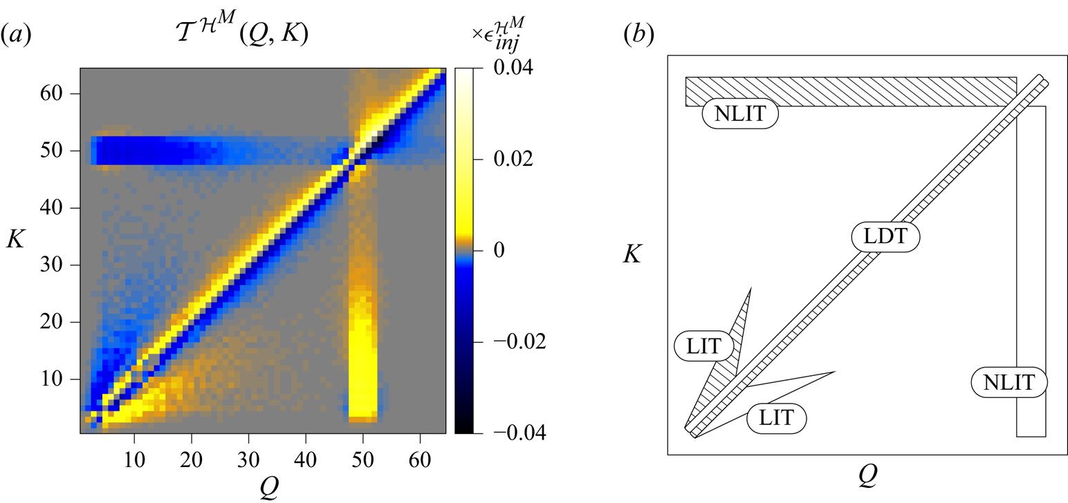
Figure 2( $a$) shows the general aspect of the shell-to-shell magnetic helicity transfers
 ${\mathcal {T}}^{{{\mathcal {H}}^M}}(Q,K)$ for the M8c run. As expected, figure 2 is antisymmetric about the main diagonal. A positive value (yellow/bright colour) above the diagonal means a positive transfer from shell
 $Q< K$ to shell
 $K$, that is, a direct transfer, whereas a negative value (blue/dark colour) above the diagonal means an inverse transfer, and vice versa for the values below the diagonal. The farther from the diagonal, the more distant the shells
 $K$ and
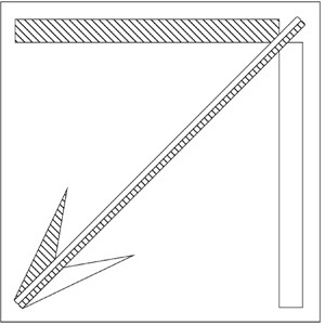
 $Q$ are, which indicates the transfers’ level of locality. Since a linear binning of the shells is chosen here, care has to be taken when interpreting the figures, since such a binning may lead to an overestimation of the transfers’ non-locality (Aluie & Eyink Reference Aluie and Eyink2010; Aluie Reference Aluie2017; Grete et al. Reference Grete, O'Shea, Beckwith, Schmidt and Christlieb2017). A linear binning is chosen here in order to see better the different features, since a logarithmic binning would leave only few shells. For visualisation purposes also, the colour bar extremes are smaller than the extremes of the transfer functions. The aim of the two-dimensional plots is indeed to present a qualitative behaviour regarding the strength, direction and locality of the transfers. Cuts along one direction are shown when a more quantitative aspect needs to be underlined. Three phenomena can thus be distinguished in the general picture of a magnetic helicity inverse transfer as sketched in figure 2(
 $b$): a local inverse transfer (LIT; corresponding to the ‘wings’ in the lower left corner close to the diagonal), a non-local inverse transfer (NLIT; corresponding to the horizontal and vertical rectangles) and a local direct transfer (LDT; along the diagonal). Test simulations have shown that the NLIT stripes at the electromotive forcing scale are not artefacts due to interactions between the mechanical and electromotive drivings but are indeed present because of small-scale magnetic helicity excess, whether the forcing terms are switched on or not.
( $a$) Magnetic helicity transfer rates from shell
 $Q$ to shell
 $K$ for the M8c run, at an instant when
 ${\mathcal {I}}_{{{\mathcal {H}}^M}} \approx {L}/{10}$. (
 $b$) Sketch of these transfer rates explicitly showing the non-local inverse transfer (NLIT), the local transfer (LIT) and the local direct transfer (LDT).

The main aim of the next subsections is to shed some light on their respective origin.
6.1. Role of the mediating velocity field at different scales
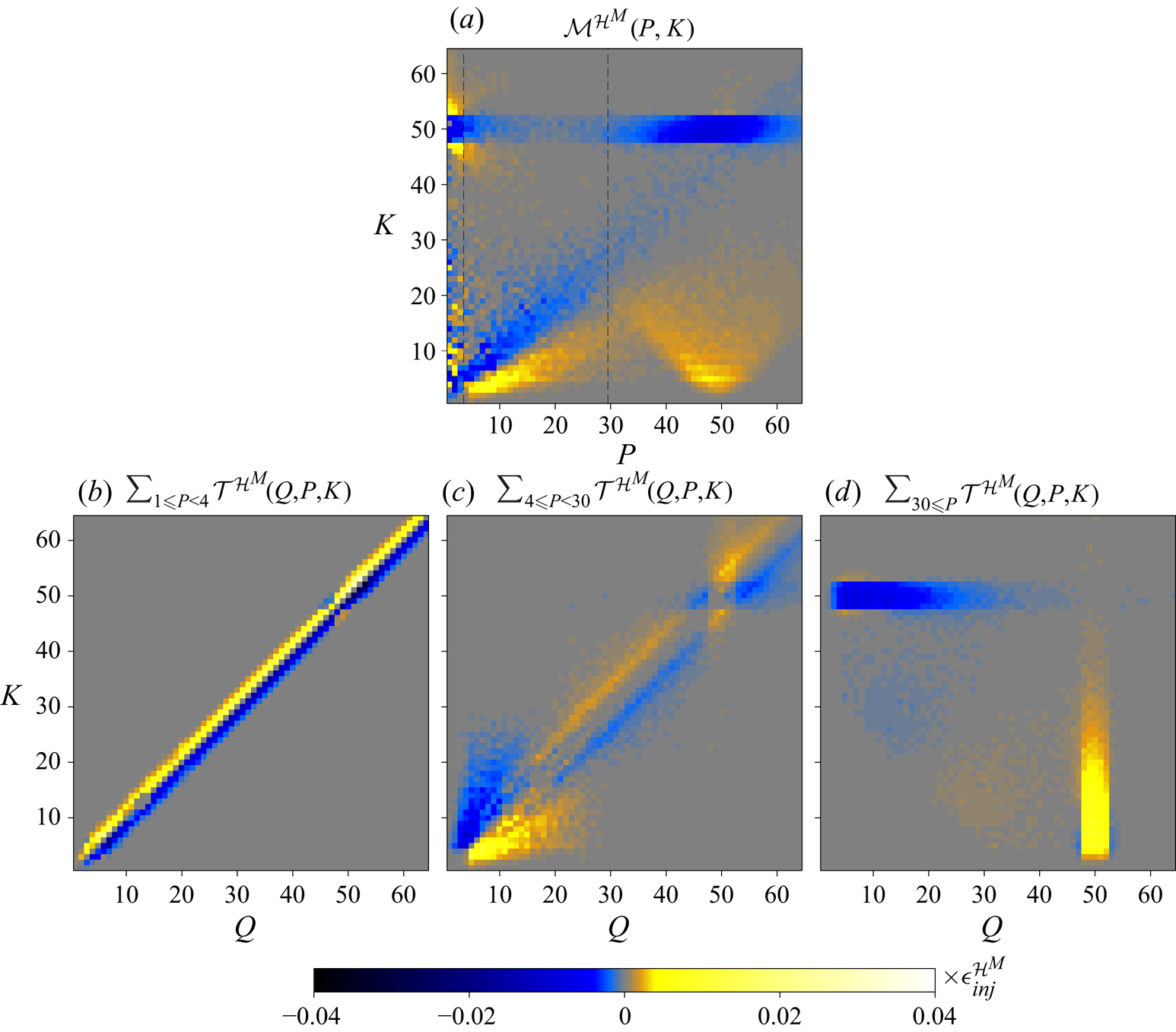
Figure 3 shows that each of the LDT, LIT and NLIT feature can be associated with different velocity scales. The function  ${\mathcal {M}}^{{{\mathcal {H}}^M}}(P,K)$ (equation (4.3)), which quantifies the importance of the mediating velocity field at shell
 $P$ with respect to transfers of magnetic helicity to shell
 $K$, allows three different regions along the
 $P$-axis to be delimited (figure 3
 $a$). The small-scale velocity field (defined as
 $30 \leq P$) transfers magnetic helicity from the electromotive driving scale to significantly larger scales, and hence corresponds to the NLIT. This process can be interpreted as the spectrally non-local merging of small-scale magnetic fluctuations with a magnetic structure of much larger size. The intermediate-scale velocity field (defined as
 $4 \leq P < 30$) transports magnetic helicity from shells
 $5 \lessapprox K \lessapprox 25$ to larger scales that are quite close spectrally (within a factor 2). This allows the interpretation of merging like-sized magnetic fluctuations and hence corresponds to the LIT. Finally, the large-scale velocity field (
 $1\leq P<4$), with alternating signs along the
 $K$-axis, is associated with the LDT. Along the same line of interpretation, the LDT would correspond to the effect of the direct cascade of kinetic and magnetic energy, i.e. the destruction of magnetic structures by advective shear exerted by the velocity field, as confirmed in § 6.4. The separation of transfer dynamics in Fourier space is confirmed on figure 3
 $(b - d)$, where the sums of
 ${\mathcal {T}}^{{{\mathcal {H}}^M}}(Q,P,K)$ for
 $P$ corresponding to the three above-mentioned velocity scales are plotted.
Role of the mediating velocity field, for run M8c at an instant when  ${\mathcal {I}}_{{{\mathcal {H}}^M}} \approx L/10$.
 $(a)$ Sum of
 ${\mathcal {T}}^{{{\mathcal {H}}^M}}(Q,P,K)$ along
 $Q$.
 $(b - d)$ Sum of
 ${\mathcal {T}}^{{{\mathcal {H}}^M}}(Q,P,K)$ along
 $P$ for different velocity field shells, showing that the three features are associated with mediation at different scales.

6.2. Helical components
Since only magnetic helicity of one sign is injected by the electromotive forcing, the dominant transfer terms are expected to be those involving the positively helical magnetic field, labelled  $+{X}+$ in § 5, with
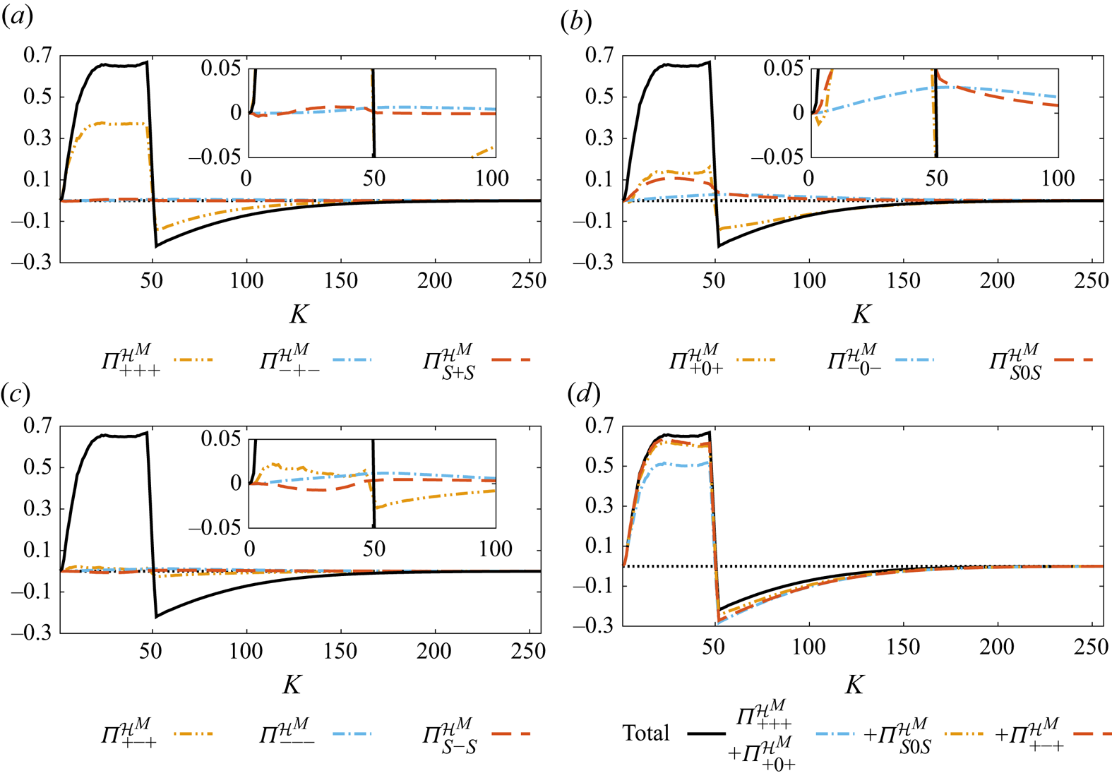
 $X \in \{+,-,0\}$ corresponding, respectively, to the positively (‘like-signed’ in the context of dominant positive magnetic helicity) and negatively (‘opposite-signed’) helical parts of the velocity field and its compressive part. These terms hence allow one to assess the role of the velocity field's helical components, as well as the role of its compressive part. Figure 4 shows the shell-integrated fluxes
 ${\varPi }^{{{\mathcal {H}}^M}}_{s_Ks_Ps_Q}(K)=\sum _{P,Q}\sum _{K_0=0}^K {\mathcal {T}}^{{{\mathcal {H}}^M}}_{s_Ks_Ps_Q}(Q,P,K_0)$ for the M8c run at an instant when
 ${\mathcal {I}}_{{{\mathcal {H}}^M}} \approx L/10$, as well as the successive sums of the dominant terms, in this order:
 $+{+}+$,
 $+{0}+$,
 $S{0}S$ and
 $+{-}+$ (figure 4
 $d$). An approximate plateau behaviour is observed. Section 6.6 discusses the dominant helical contributions at other instants. The
 $+{+}+$ and
 $+{0}+$ terms alone account for about 75 % of the inverse transfer. The plots being normalised by the magnetic helicity injection rate, a value of 1 for
 $K<48$ would mean that all the injected magnetic helicity is transferred to larger scales. This gives a rough idea of the numerical dissipation in the system: for the considered runs, about 50 %–70 % of the injected magnetic helicity is transferred to scales larger than the electromotive driving scale, where its conservation improves the larger the scale; see Teissier & Müller (Reference Teissier and Müller2021) for further details.
 $(a - c)$ The nine helically decomposed fluxes of magnetic helicity, compared to the total flux (in black), showing which ones are dominant, for the M8c run at an instant when
 ${\mathcal {I}}_{{{\mathcal {H}}^M}} \approx L/10$. The plots are normalised by the magnetic helicity injection rate. The insets are zooms close to the horizontal
 ${\varPi }^{{{\mathcal {H}}^M}}=0$.
 $(d)$ Comparison of successive sums of dominant terms.

For the M8c run, both dominant  $+{+}+$ and
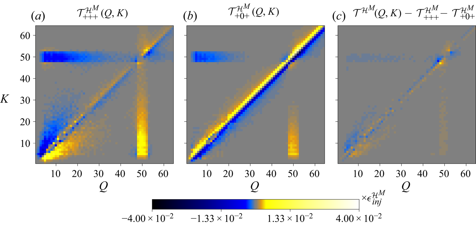
 $+{0}+$ terms, mediated by the like-signed helical velocity field and its compressive part, respectively, contribute to the NLIT in a similar way, but their contributions to the LDT and the LIT differ significantly (figure 5). The
 $+{0}+$ term takes the leading role in the LDT, but does not essentially contribute to the LIT. A more quantitative view of these aspects is available through figure 6, where cuts of figure 5 along different
 $K=K_0$ are shown.
Contributions from the  $+{+}+$ and
 $+{0}+$ terms to the magnetic helicity transfer rates for the M8c run, at an instant when
 ${\mathcal {I}}_{{{\mathcal {H}}^M}} \approx {L}/{10}$. Their sum is close to the total transfer function from figure 2 and the remaining contributions come mostly from the terms shown in figure 7.

Cuts from the two-dimensional plots of figure 5 for  $K_0 \in \{10, 30, 50\}$. The horizontal dotted line corresponds to
 $y=0$ and the vertical one to
 $Q=K_0$.

The other helical contributions are relatively small (figure 5 $c$). The three biggest remaining contributions, corresponding to the
 $+{-}+$,
 $-{0}-$ and
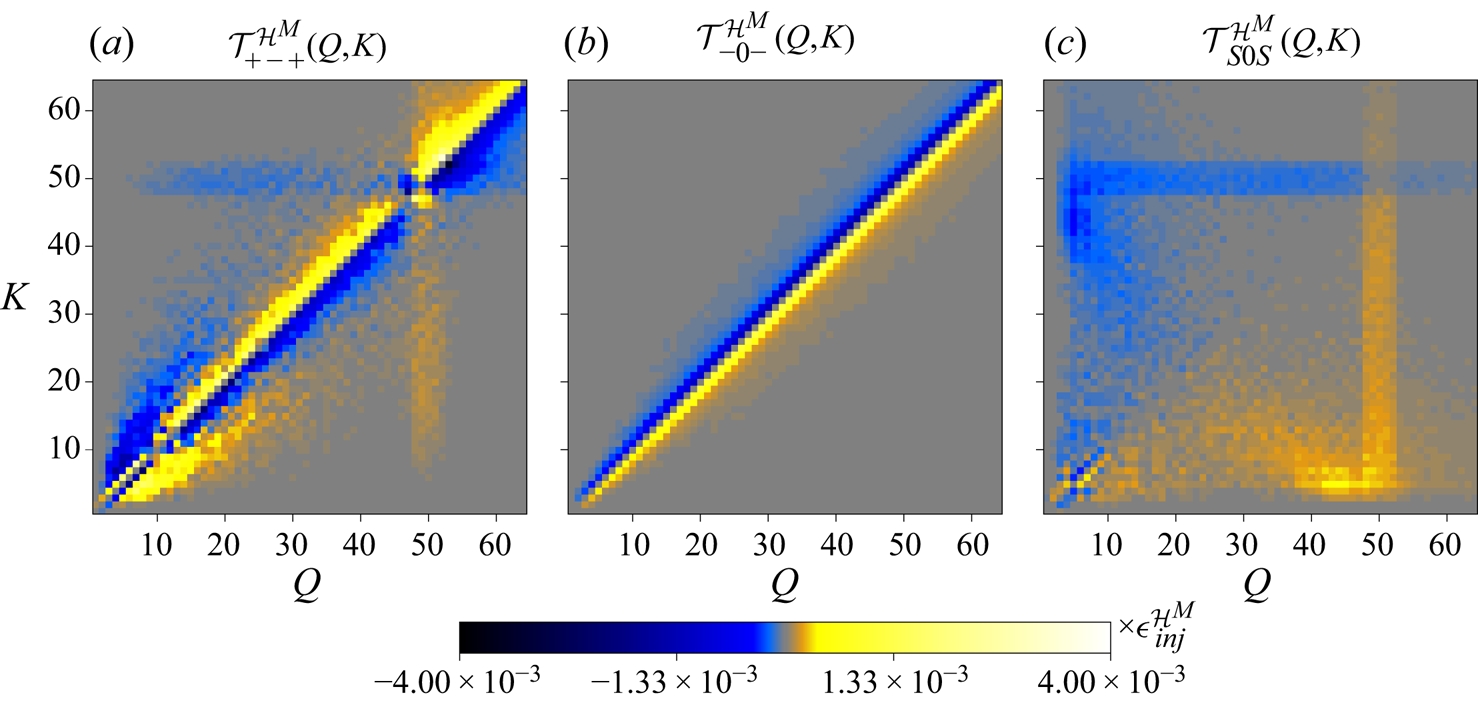
 $S{0}S$ terms, are displayed in figure 7. The
 $+{-}+$ term, mediated by the opposite-signed helical velocity field, presents a small contribution to the LIT and the LDT (please note that the colour bar extremes are a factor 10 smaller than those of figure 5), and a minor contribution to the NLIT. The
 $-{0}-$ term corresponds to a local direct transfer of negative magnetic helicity, mediated by the compressive velocity field, which results in a local inverse transfer of magnetic helicity. The heterochiral
 $S{0}S$ term exhibits a more exotic shape. Its analysis is more complex since it is the sum of two terms corresponding to different geometric helical triad factors. Although its contribution is not negligible, it is still relatively small and hence not analysed in more detail here. The remaining
 $-{-}-,\ -{+}-,\ S{+}S$ and
 $S{-}S$ helical contributions are an order of magnitude smaller as compared to the
 $+{-}+,\ -{0}-$ and
 $S{0}S$ terms and are not shown here.
Contributions from the  $+{-}+$,
 $-{0}-$ and
 $S{0}S$ terms to the magnetic helicity transfer rates for the M8c run, at an instant when
 ${\mathcal {I}}_{{{\mathcal {H}}^M}} \approx {L}/{10}$.

To summarise, for the M8c run and concentrating on the homochiral terms, the LIT is almost exclusively mediated by the solenoidal part of the velocity field ( $+{+}+$ and
 $+{-}+$ terms), with a significantly greater importance of the like-signed (
 $+{+}+$) helical part. The velocity field's compressive part (
 $+{0}+$ term) takes the leading role in the LDT, even though its solenoidal part contributes to it to a smaller extent. As for the NLIT, it is essentially mediated by both the like-signed velocity helical field and its compressive part, while the role of the opposite-signed helical velocity field is comparatively very small. The compressive part of the velocity field, which is not present in incompressible turbulence, hence enhances the direct magnetic energy cascade through shearing effects and the nonlocal merging of small-scale magnetic structures to structures of much larger size.
6.3. Interpretation through the geometric factor
The results from § 6.2 regarding the role of the  $+{+}+$,
 $+{-}+$ and
 $+{0}+$ terms can be explained through the moduli
 $G^{+++}$,
 $G^{+-+}$ and
 $G^{+0+}$ of the respective helical geometric triad factors (relations (5.5) and (5.6)), displayed in figure 8, in which panel (
 $d$) summarises the results from § 6.1. The LDT that is associated with the large-scale velocity field corresponds to
 $p \ll k \approx q$, whereas the LIT, associated with the intermediate-scale velocity field, corresponds to
 $p \approx k \approx q$. The NLIT is mediated by the small-scale velocity field, that is,
 $k \ll p \approx q$ and
 $q \ll p \approx k$.
 $(a - c)$ Triad helical geometric factor's modulus for the
 $+{+}+$,
 $+{0}+$ and
 $+{-}+$ terms, respectively (see relations (5.5) and (5.6)).
 $(d)$ Sketch showing to which regions the NLIT (non-local inverse transfer), the LIT (local inverse transfer) and the LDT (local direct transfer) correspond.

Comparison of the geometric factors’ moduli has led to the predictions that the  $+{+}+$ transfers, mediated by the velocity field of like-signed helicity, are both more efficient and more non-local than the
 $+{-}+$ ones, where the mediating field has an opposite-signed helicity in the incompressible case (Linkmann et al. Reference Linkmann, Sahoo, McKay, Berera and Biferale2017). The same idea is used here, extending these results in compressible MHD and allowing the determination of the relative importance of the
 $+{+}+$,
 $+{-}+$ and
 $+{0}+$ terms for the three NLIT, LIT and LDT features.
(1) In the region
 $k \approx p \approx q$ corresponding to the LIT, the $G^{+++}$ term is biggest, with a maximum at $3\sqrt {3}/2 \approx 2.6$ for $k=p=q$, whereas $G^{+-+}< G^{+++}$ by a factor of about 3 and $G^{+0+}$ vanishes in this region. This explains why the LIT is mediated by the like-signed helical velocity field ($+{+}+$ term) and to a lesser extent by the opposite-signed helical velocity field ($+{-}+$), but is essentially absent from the $+{0}+$ term, corresponding to a mediation by the compressive velocity field.
(2) In the region corresponding to the NLIT, both
$G^{+++}$ and $G^{+0+}$ are high, which explains why the like-signed helical velocity field and its compressive part play an important role for this feature. However, for $k\approx q$, $G^{+0+}$ is vanishing, which explains why the NLIT is more non-local for the compressive velocity field as compared to the like-signed helical one – see figure 6$(c)$, where the inverse transfer for the $+{0}+$ term is visible only for shells $K \leq 30$ whereas it is visible for all shells $K \leq 50$ for the $+{+}+$ one. As for $G^{+-+}$, it is vanishing in this region so that the role of the opposite-signed helical velocity field is small for this feature.(3) Finally, all three terms have a non-vanishing geometric factor at low
$p$, corresponding to the large-scale velocity field. This is why they all contribute to the LDT. The reason why the compressive velocity field plays the leading role for this feature cannot be explained solely by the fact that more energy is associated with it, as compared to the positively or negatively helical components (see figure 9$d$). Indeed, for the M11s run (see § 6.5), the contributions of the $+{+}+$ and $+{0}+$ terms to the LDT have similar amplitudes, even though significantly more energy is contained in the positively helical velocity field for this run (figure 9$b$). The $+{0}+$ term is favoured geometrically because (i) on the $q=p+k$ and $q=-p+k$ lines, $G^{+0+}=2$, whereas $G^{+++}=G^{+-+}=0$ and (ii) the $q=k$ horizontal line, where $G^{+++}$ and $G^{+-+}$ are high at low $p$, does not play a role for shell-to-shell transfers between shells $K$ and $Q$ since ${\mathcal {T}}^{{{\mathcal {H}}^M}}(K,K)=0$. However, as shown in § 6.5, even though the $+{0}+$ term is favoured geometrically, it can play a less important role depending on the energy repartition among the helical velocity components.


Repartition of the specific kinetic energy in the helical components for all the extreme runs, at an instant when  ${\mathcal {I}}_{{{\mathcal {H}}^M}} \approx L/10$.

The analysis above assumed that the helically decomposed shell-to-shell transfer rates  ${\mathcal {T}}^{{{\mathcal {H}}^M}}_{s_Ks_Ps_Q}(Q,P,K)$ have a similar shape as the single triad geometric factors’ one, which is of course not guaranteed. The magnetic helicity at a wavevector
 $\boldsymbol {k}$ can be written
 $H^M_{\boldsymbol {k}}=({1}/{k})(|{{{}\hat {b}}^+_{\boldsymbol {k}}}|^2-|{{{}\hat {b}}^{-}_{\boldsymbol {k}}}|^2)$, with
 ${{\boldsymbol {{{{}\hat {b}}}}}^{\pm }_{\boldsymbol {k}}}={{{}\hat {b}}^{\pm }_{\boldsymbol {k}}}\boldsymbol {{{\hat {h}}}}^\pm _{\boldsymbol {k}}$ the helically decomposed magnetic field, whose time evolution is governed by
 \begin{equation} \partial_t H^M_{\boldsymbol{k}}=\frac{1}{k}( 2\,{\mathrm{Re}}({{{}\hat{b}}^+_{\boldsymbol{k}}}^* \partial_t {{{}\hat{b}}^+_{\boldsymbol{k}}} + {{{}\hat{b}}^{-}_{\boldsymbol{k}}}^* \partial_t {{{}\hat{b}}^{-}_{\boldsymbol{k}}})), \end{equation}
where Re(z) denotes the real part of the complex number z. Hence, according to relation (5.4), the magnetic helicity transfers depend, apart from the phase information and the geometric factor, on the moduli of the interacting helical modes in the triads. In order to isolate the geometric factors’ role, slices at particular K 0 of the different helical components  ${\mathcal{T}}^{{{\mathcal{H}}^M}}_{{s_Ks_Ps_Q}}(Q,P,{K_0})$ normalised by the typical interacting fields’ moduli are considered:
 \begin{equation} {\mathcal{N}}^{{{\mathcal{H}}^M}}_{{s_Ks_Ps_Q}}(Q,P,{K_0})=\frac{{\mathcal{T}}^{{{\mathcal{H}}^M}}_{{s_Ks_Ps_Q}}(Q,P,{K_0})}{2\sqrt{2E^{M,s_K}_{K_0}E^{V,s_P}_P E^{M,s_Q}_Q}}, \end{equation}
with  $E^{M,s_Q}_Q$ the power spectrum of the magnetic field
 $s_Q$-helical part (obtained by projecting
 $\boldsymbol {{{{}\hat {b}}}}$ on the
 $(\boldsymbol {{{{\hat {h}}}^{s_q}_{\boldsymbol {q}}}})$ helical eigenvectors in Fourier space) and similarly for the other two energetic contributions. An average of all the
 $K \in [5,50]$ slices of
 ${\mathcal {N}}^{{{\mathcal {H}}^M}}_{{s_Ks_Ps_Q}}(Q,P,{K})$ in one plot is shown in figure 10. This plot has been obtained by normalising, resizing and merging the 46 slices present in this wavenumber shell range, through the procedure described in Appendix B.
Average of the 46 slices of  ${\mathcal {N}}^{{{\mathcal {H}}^M}}_{{s_Ks_Ps_Q}}(Q,P,{K_0})$ for
 $K_0 \in [5,50]$, obtained through the procedure described in Appendix B. Each plot is normalised by its own maximum absolute value.

The geometric triad factors’ shape is very well reflected in figure 10 for the  $+{+}+,\ +{-}+$ and
 $+{0}+$ terms. In this figure, the blue/yellow corner at small
 $P/K$ corresponds to the LDT: it is negative for
 $Q/K>1$ and positive for
 $Q/K<1$, which means that magnetic helicity is transferred from larger to smaller scales, whereas the reversal of colours at higher
 $P/K$ corresponds to inverse transfers (LIT and NLIT).
This illustrates why the geometric triad factor moduli govern the role and relative importance of the dominant helical contributions with respect to shell-to-shell magnetic helicity transfers.
6.4. Energetic transfers
Using the decomposition of the magnetic helicity transfer function in contributions related to energetic transfers (relations (4.13)–(4.15), plotted in figure 11) allows one to see that the LDT is essentially associated with a direct cascade of magnetic energy within the magnetic energy reservoir (hereafter labelled as  $B \leftrightarrow B$ exchanges). This magnetic energy cascade is due to the advective flux of magnetic helicity and magnetic pressure. On the contrary, the LIT and the NLIT are associated with both
 $B \leftrightarrow B$ and
 $V \leftrightarrow B$ exchanges (where
 $V \leftrightarrow B$ represents the effects of transfers between the magnetic and kinetic energy reservoirs). As expected from the analysis in § 6.2, the LIT is mostly associated with
 $V \leftrightarrow B$ transfers due to magnetic tension (shear Alfvénic effects), which dominate over the
 $B \leftrightarrow B$ ones. The NLIT is caused by all three mechanisms (advection, magnetic tension and magnetic pressure) and linked with both
 $B \leftrightarrow B$ and
 $V \leftrightarrow B$ transfers.
Decomposition of the magnetic helicity transfer rate from shell  $Q$ to shell
 $K$ (panel
 $(a)$, which is the same as figure 2) in different contributions:
 $(b)$ associated with
 $B \leftrightarrow B$ exchanges,
 $(c)$ associated with
 $V \leftrightarrow B$ exchanges, the latter being the sum of
 $(d)$ contributions through the magnetic tension and
 $(e)$ through the magnetic pressure.

6.5. Other runs
The other runs, M01s4, M11s and M1c, are also considered at an instant when  ${\mathcal {I}}_{{{\mathcal {H}}^M}}\approx L/10$. Even though the compressibility of these runs extends over a wide range, they exhibit a lot of common properties with the M8c run: the same three features (LDT, LIT and NLIT) are present and mediated by the velocity field at the same scales. The LDT is always mostly associated with
 $B \leftrightarrow B$ exchanges, whereas the LIT and NLIT are associated with both
 $B \leftrightarrow B$ and
 $V \leftrightarrow B$ exchanges. The differences observed are essentially quantitative and concern the different helical contributions’ importance. They can be explained through the energy repartition in the velocity field's helical components, given in figure 9.
For the M11s run (figure 12), both the velocity field's compressive and like-signed helical parts contribute in equal proportions to the LDT, contrary to the situation for the M8c run. For this run, indeed, the positively helical velocity field entails significantly more energy  $E^{V,+}$ than its compressive part
 $E^{V,0}$ at large scales. This confirms that the compressive velocity field is indeed geometrically favoured for the LDT.
 $(a - c)$ Magnetic helicity transfer rates between the shells
 $Q$ and
 $K$ and their greatest helical contributions for the M11s run at an instant in time when
 ${\mathcal {I}}_{{{\mathcal {H}}^M}} \approx {L}/{10}$.
 $(d)$ Cuts of panels
 $(a - c)$ at
 $K_0=30$. The transfers are expressed in units of the magnetic helicity injection rate
 ${\epsilon ^{{{\mathcal {H}}^M}}_{inj}}$.

The other extreme happens for the M1c run, for which the  $E^{V,0}/E^{V,+}$ ratio is very large at large scales and small at small scales. As a consequence, the LDT has a very large magnitude as compared to the NLIT and the LIT (figure 13
 $(a - c)$, where the colour bar extremes in panel
 $(b)$ are an order of magnitude smaller) and the
 $+{0}+$ term does not contribute much to the NLIT (figure 13
 $c,\,f$).
 $(a - c)$ Magnetic helicity transfer rates between the shells
 $Q$ and
 $K$ and their greatest helical contributions for the M1c run at an instant when
 ${\mathcal {I}}_{{{\mathcal {H}}^M}} \approx {L}/{10}$. Please note that the extremes of the colour bar of panel
 $(b)$ are an order of magnitude lower as compared to panels
 $(a)$ and
 $(c)$.
 $(d - f)$ Cuts of panels
 $(a - c)$ at
 $K_0=10$,
 $K_0=30$ and
 $K_0=50$, respectively. The transfers are expressed in units of the magnetic helicity injection rate
 ${\epsilon ^{{{\mathcal {H}}^M}}_{inj}}$.

Lastly, the LDT is carried by both helical components of the velocity field for the subsonic M01s4 run (figure 14), since there is only a negligible amount of energy in the compressive velocity field. For this run, both  $+{+}+$ and
 $+{-}+$ terms have the same importance with respect to the LDT because similar amounts of energy are present in the positively and negatively helical parts of the velocity field and the magnitudes of the geometric factors
 $G^{+++}$ and
 $G^{+-+}$ (see relation (5.5)) have very close values for
 $p \ll k \approx q$.
 $(a - c)$ Magnetic helicity transfer rates from shell
 $Q$ to shell
 $K$ for the M01s4 run at an instant when
 ${\mathcal {I}}_{{{\mathcal {H}}^M}} \approx {L}/{10}$, as well as the biggest helical contributions.
 $(d)$ Cuts of panels
 $(a - c)$ at
 $K_0=30$. The transfers are expressed in units of the magnetic helicity injection rate
 ${\epsilon ^{{{\mathcal {H}}^M}}_{inj}}$.

6.6. Discussion: other instants in time and transient effects
The results presented in this work are based on a single snapshot, taken at an instant in time when the magnetic helicity peak is still relatively far from the largest available scales ( ${\mathcal {I}}_{{{\mathcal {H}}^M}}\approx L/10$) so as to avoid finite-size effects. Figure 15 shows the transfers and fluxes at different instants in time for the M8c run and can be compared directly with figure 4. At a later instant in time, when
 ${\mathcal {I}}_{{{\mathcal {H}}^M}}\approx L/6$, the main instant considered for the study of spectral scaling laws in Teissier & Müller (Reference Teissier and Müller2021), the general behaviour looks qualitatively very similar. At a clearly earlier instant in time,
 ${\mathcal {I}}_{{{\mathcal {H}}^M}}\approx L/40$, when no approximate plateau behaviour is observed and no large-scale structure has emerged yet, the transfers are significantly different. Even though non-local transfers are already present, local transfers are dominant, in agreement with Alexakis et al. (Reference Alexakis, Mininni and Pouquet2006) and Linkmann & Dallas (Reference Linkmann and Dallas2016), where non-local transfers from the electromotive forcing directly to the largest energy-containing scales only appear at later times. It can be noted in passing that the heterochiral
 $S{0}S$ term plays a negligible role at such an early instant, and becomes important only later.
 $(a)$ Time evolution of the magnetic helicity transfer Fourier spectra
 $\sum _{P,Q}{\mathcal {T}}^{{{\mathcal {H}}^M}}(Q,P,K)$ for the M8c run; five snapshots equally spaced in time between instants when
 ${\mathcal {I}}_{{{\mathcal {H}}^M}}\approx L/40$ and
 ${\mathcal {I}}_{{{\mathcal {H}}^M}}\approx L/6$.
 $(b,c)$ Magnetic helicity transfer spectra at the extreme instants of panel
 $(a)$ and some important helical contributions.
 $(d - f)$ Same as
 $(a - c)$ but with the magnetic helicity fluxes
 ${\varPi }^{{{\mathcal {H}}^M}}(K)=\sum _{K_0=0}^K {\mathcal {T}}^{{{\mathcal {H}}^M}}(K)$.

The finite size of the numerical system in combination with the deliberately chosen lack of large-scale dissipation to avoid artefacts in the nonlinear flux measurements does not allow us to obtain a standard statistically stationary turbulent state. Ensemble averaging, an alternative ansatz, would be numerically too costly for the present isothermal system. Therefore, lurking dangers to avoid are the dependence of our measurements on the chosen point in time and on the initial conditions. The presence of the inherently non-local dynamics of turbulent magnetic fields makes the latter aspect relevant for almost any kind of MHD simulation or experiment. Indeed, considerations in Teissier & Müller (Reference Teissier and Müller2021), from which the extreme runs are considered in the present work, show that the observed spectral scaling laws strongly depend on the choice of the initial frame for compressively driven runs with turbulent Mach numbers close to 5, labelled M5cA and M5cB. This is an indication that the snapshots considered could still be in a transient phase.
Nevertheless, the main results exposed in that work, the dynamical balance between shearing and stretching and the scaling laws of appropriately chosen quantities (e.g. considering the Alfvén velocity in place of the magnetic field), have been shown to be valid over a wider range of compressibility, to be roughly constant as the systems are evolved in time, and to be independent of the chosen initial conditions (runs M5cA and M5cB). They have furthermore been confirmed at higher resolutions.
Single snapshot data are considered in the present work, too. However, the qualitatively very similar behaviour of the flows over a wide range of compressibility (extending from Mach 0.1 solenoidally driven close to Mach 8 compressively driven) as well as the explanation of the results through the geometric helical factor and the energy contents in the helical modes are strong arguments that hint at the robustness of the presented main results of this work when considering the cautionary remarks above.
7. Conclusion
The helically decomposed shell-to-shell analysis reveals the presence of three distinct phenomena occurring in the global picture of the inverse transfer of magnetic helicity and sheds some light on their origin. Since one sign of magnetic helicity dominates the system at all scales, the role of the different helical components of the velocity field as well as that of its compressive part can be distinguished. The analysis has been performed on particular states taken from direct numerical simulations of magnetic helicity inverse transfer in compressible isothermal MHD flows (Teissier & Müller Reference Teissier and Müller2021). The range of Mach numbers varies from subsonic to r.m.s. Mach numbers of the order of 10, with either a purely solenoidal or compressive mechanical large-scale forcing. The results are consistent with previous research done in the incompressible case regarding the transfer's direction and locality (Alexakis et al. Reference Alexakis, Mininni and Pouquet2006) and relative strength and locality of triad interactions involving the like-signed and opposite-signed helical part of the velocity field (Linkmann et al. Reference Linkmann, Sahoo, McKay, Berera and Biferale2017).
For all the runs considered, a local inverse transfer (LIT), a non-local inverse transfer (NLIT) and a local direct transfer (LDT) are observed:
(i) The LIT is caused predominantly by magnetic stretching involving the solenoidal velocity field at intermediate scales, i.e. shear Alfvénic fluctuations. The like-signed helical velocity field plays the dominant role here. It is associated with both magnetic
$\leftrightarrow$ magnetic ($B \leftrightarrow B$) and kinetic $\leftrightarrow$ magnetic ($V \leftrightarrow B$) energetic exchanges.(ii) The leading role in the NLIT is taken by the small-scale velocity field, through both the like-signed helical velocity field and its compressive part.
(iii) Finally, the LDT is caused by the large-scale velocity field. It is essentially associated with a direct cascade of kinetic and magnetic energy. The compressive part of the velocity field is geometrically favoured for the LDT even though both velocity helical components, which have geometrically a similar importance, can take the leading role depending on the specific kinetic energy repartition among the helical and compressive modes.


Thus the velocity field's compressive part, which is not present in the incompressible case, plays an important role in the LDT and the NLIT, which affects the magnetic helicity scaling properties (Teissier & Müller Reference Teissier and Müller2021).
The locality and strength of these phenomena can be explained surprisingly well by the geometric triad helical factors (Waleffe Reference Waleffe1992), which have been extended for compressible MHD.
Since magnetic helicity is not sign-definite, in astrophysical systems of interest, magnetic helical components of mixed signs are expected to be present. In this context, the heterochiral terms (labelled  $S{+}S,\ S{-}S$ and
 $S{0}S$) may play a greater role, even though they are more difficult to interpret (Teissier Reference Teissier2020). In particular, in the present work, even though magnetic helicity of one sign dominates the system, the heterochiral term
 $S{0}S$ associated with the compressive velocity field plays a relatively small but not negligible role at high compressibility, in contrast to the other
 $S{+}S$ and
 $S{-}S$ heterochiral terms. This would deserve further studies. Nevertheless, the study presented here, which focuses on the dominant homochiral terms, provides insights that should help the interpretation of future results in more general cases.
Acknowledgements
The authors acknowledge the North-German Supercomputing Alliance (HLRN) for providing HPC resources that have contributed to the research results reported in this paper. Computing resources from the Max Planck Computing and Data Facility (MPCDF) are also acknowledged.
Funding
J.-M.T. gratefully acknowledges support by the Berlin International Graduate School in Model and Simulation based Research (BIMoS).
Declaration of interests
The authors report no conflict of interest.
Appendix A. Geometric factor derivation
The geometric factor appearing in relation (5.4) has been derived in Waleffe (Reference Waleffe1992) in the incompressible case. The derivations are reviewed here, keeping the same notation as shown in figure 16. The helical eigenvectors  $\boldsymbol {{{{\hat {h}}}^{s_k}_{\boldsymbol {k}}}}, \boldsymbol {{{{\hat {h}}}^{s_p}_{\boldsymbol {p}}}}$ and
 $\boldsymbol {{{{\hat {h}}}^{s_q}_{\boldsymbol {q}}}}$ are expressed for each triad in a well-chosen basis:
 \begin{equation} \boldsymbol{{{{\hat{h}}}^{s_m}_{\boldsymbol{m}}}}= \textrm{e}^{\textrm{i}s_m\phi_m}({\boldsymbol \lambda}+\textrm{i}s_m{\boldsymbol \mu}_{\boldsymbol{m}}), \end{equation}
with  $\boldsymbol {m} \in \{\boldsymbol {k},\boldsymbol {p},\boldsymbol {q}\}$,
 $\phi _m$ a certain angle and
 ${\boldsymbol \lambda }$ and
 ${\boldsymbol \mu }_{\boldsymbol {m}}$ the unitary vectors:
 $$\begin{gather} {\boldsymbol \lambda} = \frac{\boldsymbol{k} \times \boldsymbol{p}}{|\boldsymbol{k} \times \boldsymbol{p}|}=\frac{\boldsymbol{p} \times \boldsymbol{q}}{|\boldsymbol{p} \times \boldsymbol{q}|}=\frac{\boldsymbol{q} \times \boldsymbol{k}}{|\boldsymbol{q} \times \boldsymbol{k}|}, \end{gather}$$
 $$\begin{gather}{\boldsymbol \mu}_{{\boldsymbol{m}}} = \frac{{\boldsymbol{m}} \times {\boldsymbol \lambda}}{|{\boldsymbol{m}}|}. \end{gather}$$
Definition of the notation for the derivations of the geometric triad factor. Redrawn from Waleffe (Reference Waleffe1992).

In the incompressible case ( $s_k,s_p,s_q \in \{+,-\}$), this gives after some algebra the geometric triad factor (Waleffe Reference Waleffe1992):
 \begin{align} g^{s_k,s_p,s_q}_{k,p,q} &= (\boldsymbol{{{{\hat{h}}}^{s_p*}_{\boldsymbol{p}}}} \times \boldsymbol{{{{\hat{h}}}^{s_q*}_{\boldsymbol{q}}}}) \boldsymbol{\cdot} \boldsymbol{{{{\hat{h}}}^{s_k*}_{\boldsymbol{k}}}}, \end{align}
 \begin{align} &={-}\textrm{e}^{-\textrm{i} (s_k \phi_k + s_p \phi_p + s_q \phi_q)}s_ks_ps_q(s_k \sin(\alpha_k)+s_p \sin(\alpha_p)+s_q \sin(\alpha_q)), \end{align}
 \begin{align} &= \textrm{e}^{-\textrm{i} \phi_s}\frac{s_ks_ps_q(s_k k+s_p p+s_q q)\sqrt{2k^2p^2+2p^2q^2+2q^2k^2-k^4-p^4-q^4}}{2kpq}, \end{align}
with  $\phi _s=(s_k \phi _k + s_p \phi _p + s_q \phi _q)$. The last equality is obtained by using the law of sines and Heron's formula.
In the compressible case, when  $s_p=0,\ s_k=S \in \{+,-\},\ s_q=\pm S$, the geometric factor becomes
 \begin{align} g^{s_k=S,0,s_q={\pm} S}_{k,p,q} &= \left(\frac{\boldsymbol{p}}{p} \times \boldsymbol{{{{\hat{h}}}^{s_q*}_{\boldsymbol{q}}}}\right) \boldsymbol{\cdot} \boldsymbol{{{{\hat{h}}}^{s_k*}_{\boldsymbol{k}}}}, \end{align}
 \begin{align} &= {S}\textrm{{i}}\textrm{{e}}^{{-S}\textrm{{i}}(\phi_k\pm\phi_q)} (\cos(\alpha_q)\mp \cos(\alpha_k)), \end{align}
 \begin{align} &= {S}\textrm{i}\textrm{e}^{{-S}\textrm{i}(\phi_k\pm\phi_q)} \frac{(q\mp k)(p^2-k^2-q^2\mp 2qk)}{2kpq}, \end{align}
where the last equality is obtained using the cosine rule  $\cos (\alpha _k)=({kp^2+kq^2-k^3})/{2kpq}$.
Appendix B. Technical details: merging transfer functions’ slices
Figure 10 is obtained by merging the  ${\mathcal {N}}^{{{\mathcal {H}}^M}}_{{s_Ks_Ps_Q}}(Q,P,{K})$ slices (relation (6.2)) for
 $K \in [5,50]$ through the following procedure (see figure 17):
(1) Each slice is considered as a ‘picture’ and is resized so that the angles
$P=K$ and $Q=K$ arrive at the same location for each of them. The slices are normalised by the maximum of their respective absolute value so that they all have the same weight in the final merged picture. Only the slices starting $K=5$ are considered since low-$K$ slices are more imprecisely resized, causing square-like artefacts.(2) For each
$(P,Q)$ coordinate, the sum of all resized pictures is considered, leading to their superposition, the new ‘picture’ $S$.(3) Each
$(P,Q)$ coordinate in the $S$ picture is normalised by the number of pictures that contributed to it (it differs for each point since all resized pictures occupy a different domain; see figure 17).(4) The obtained
$S$ is finally normalised by its maximum absolute value.


Illustration of the algorithm generating figure 10. ( $a$) Three slices being merged. (
 $b$) After resizing so that their angles coincide. (
 $c$) The final merged picture. The sum of the red and blue bands from the top and middle pictures gives the purple band, which is normalised by a factor 2, since only two of the three slices contributed to it. The smaller orange square is normalised by a factor 3 since it comes from all three slices.