1. Introduction
Particle transport in channel flow or duct flow of non-Newtonian fluids is widely observed in industrial and biological applications, such as red blood cells in blood vessels (Beris et al. Reference Beris, Horner, Jariwala, Armstrong and Wagner2021), droplets and particles separation via microfluidic chips (D’Avino et al. Reference D’avino, Del Greco and Maffettone2017) and hydraulic fracturing (Barbati et al. Reference Barbati, Desroches, Robisson and Mckinley2016). In practice, the addition of small amounts of polymers can significantly modify the rheological properties of simple Newtonian fluids such as water, which is widely used in food and chemical engineering (Bonn et al. Reference Bonn, Denn, Berthier, Divoux and Manneville2017). The influence of the viscoelastic and shear-thinning properties on the motion of particles in duct flow has always attracted attention (Lashgari et al. Reference Lashgari, Ardekani, Banerjee, Russom and Brandt2017; Liu et al. Reference Liu2017; Saccone, Marchioli & Marchis Reference Saccone, Marchioli and Marchis2022; Habibi et al. Reference Habibi, Iqbal, Ardekani, Chaparian, Brandt and Tammisola2025; Hu et al. Reference Hu, Lin, Yu, Lin and Xia2025).
Lateral migration of particles and cells in duct flow has drawn considerable interest (Kahkeshani, Haddadi & di Carlo Reference Kahkeshani, Haddadi and di Carlo2016; Nakayama et al. Reference Nakayama, Yamashita, Yabu, Itano and Sugihara-Seki2019; Manoorkar & Morris Reference Manoorkar and Morris2021; Sojwal & Morrris Reference Sojwal and Morris2021; Zhou et al. Reference Zhou, Dou, Timilsina, Xu and Li2021). In Newtonian fluids, the classical Segré–Silberberg effect described how spherical particles in a circular channel flow focused near the wall to seek the equilibrium position (Segré & Silberberg Reference Segré and Silberberg1961). At Re ≤ 100, four equilibrium positions exist at each wall bisector for the migration of spherical particles in a square channel, and the equilibrium position shifts closer to the wall with increasing Re (Abbas et al. Reference Abbas, Magaud, Gao and Geoffroy2014; Miura, Itano & Sugihara-Seki Reference Miura, Itano and Sugihara-Seki2014; Shichi et al. Reference Shichi, Yamashita, Seki, Itano and Sugihara-Seki2017; Hu et al. Reference Hu, Yu, Zhu, Bao, Lin, Tu and Lin2024b ).
In viscoelastic fluids, shear-induced lift force (Saffman Reference Saffman1965; Feng, Hu & Joseph Reference Feng, Hu and Joseph1994; Matas, Morris & Élisabeth Reference Matas, Morris and Élisabeth2009), wall-induced lift force and fluid elasticity (Raoufi et al. Reference Raoufi, Mashhadian, Niazmand, Asadnia, Razmjou and Warkiani2019) determine the final equilibrium position. Leshansky et al. (Reference Leshansky, Bransky, Korin and Dinnar2007) first found that viscoelasticity could focus spherical particles towards the centre of a circular channel at low Reynolds numbers. When the fluid inertia was negligible, del Giudice et al. (Reference del Giudice, D’avino, Greco, Maffettone and Shen2018) found the first normal stress difference in viscoelastic fluid yielded an elastic lift, which would push particles towards the corner and channel centreline with low-shear-rate regions. Synergistic elasto-inertial effects can improve the particle separation efficiency in a viscoelastic fluid (Lim et al. Reference Lim, Ober, Edd, Desai, Neal, Bong, Doyle, Mckinley and Toner2014; Seo, Kang & Lee Reference Seo, Kang and Lee2014). Kim & Kim (Reference Kim and Kim2016) and Raoufi et al. (Reference Raoufi, Mashhadian, Niazmand, Asadnia, Razmjou and Warkiani2019) found that fluid inertia could focus particles at the channel centreline and reduce the number of particles at the corners of the square duct. Yu et al. (Reference Yu, Wang, J. and Hu2019) discovered that spherical particles in a square duct flow of Oldroyd-B fluids migrated towards the corner (CO), wall bisector, diagonal line (DL) and channel centreline (CC) equilibrium positions.
The aforementioned studies considered spherical particles; the migration of non-spherical particles in the duct flow of viscoelastic fluids has recently received considerable attention (Tai, Wang & Narsimhan Reference Tai, Wang and Narsimhan2020; Del Giudice & D’Avino Reference del Giudice and D’avino2025). In a viscoelastic fluid with negligible fluid inertia, D’Avino et al. (Reference D’avino, Hulsen, Greco and Maffettone2019) showed that the prolate spheroid would migrate to the channel centreline or the closest wall; however, the influence of particle shape and size were not reported. When the inertial effect in a square duct flow of Oldroyd-B fluid is obvious, Li, Xu & Zhao (Reference Li, Xu and Zhao2024) showed that the oblate spheroid kept an oscillating migration behaviour, and the critical elastic number determined the final equilibrium position. Hu et al. (Reference Hu, Lin, Zhu, Yu, Lin and Li2024a ) reported six (five) types of rotational behaviours for the elasto-inertial migration of prolate (oblate) spheroids in an Oldroyd-B fluid, where the equilibrium position rapidly decreased upon increasing the elastic number. The complex rotational motion makes it difficult to predict the equilibrium position of non-spherical particles; therefore, the rotational diameter is often selected (Hur, Tse & di Carlo Reference Hur, Tse and di Carlo2010; Masaeli et al. Reference Masaeli, Sollier, Amini, Mao, Camacho, Doshi, Mitragotri, Alexeev and di Carlo2012; Su, Chen & Hu Reference Su, Chen and Hu2018). Hu et al. (Reference Hu, Kang, Lin, Lin, Bao and Zhu2023) showed that equivalent spheres with the same rotational diameter as oblate spheroids could be used to predict the equilibrium position of the latter in a duct flow of inelastic power-law fluids.
The aforementioned works mainly considered the migration of particles in purely elastic fluids without shear-thinning. However, the detailed influence of fluid rheology and inertia on the rotational behaviour of spheroidal particles in the duct flow of shear-thinning viscoelastic fluids was not fully explored. Several viscoelastic fluids exhibit shear-thinning characteristics, and the non-negligible second normal stress difference can induce secondary flows in a non-circular duct flow (Debbaut & Dooley Reference Debbaut and Dooley1999; Yue, Dooley & Feng Reference Yue, Dooley and Feng2008; Habibi et al. Reference Habibi, Iqbal, Ardekani, Chaparian, Brandt and Tammisola2025). The competition between viscoelasticity-induced migration and secondary flows further alters the motion behaviour of particles. In a Giesekus fluid with negligible fluid inertia, Villone et al. (Reference Villone, D’avino, Hulsen, Greco and Maffettone2013) showed that the secondary flow trapped some spherical particles in the vortex structure, with the particles following a spiralling trajectory. Li, Mckinley & Ardekani (Reference Li, Mckinley and Ardekani2015) showed that spherical particles maintained the CC equilibrium position in an Oldroyd-B fluid with strong elasticity, while the shear-thinning effect in a Giesekus fluid promoted particle migration closer to the wall. Wang, Yu & Lin (Reference Wang, Yu and Lin2018) found that spherical particles in Giesekus fluids would focus either at the channel centre or at the nearest corner of a rectangular duct under low fluid inertia, whereas the particles focused at the bisector of the short walls when the inertial and elastic effects were non-negligible. For non-spherical particles, Langella et al. (Reference Langella, Franzino, Maffettone, Larobina and D’avino2023) showed experimentally that prolate spheroids focused at the channel centre at the maximum flow rate forRe = 0.0007, and that the prolate spheroids were less likely to migrate towards the wall compared with spheres, even in a shear-thinning viscoelastic fluid. However, their studies did not fully explore the effect of fluid inertia and particle shape. Naseer et al. (Reference Naseer, Izbassarov, Ahmed and Muradoglu2024) found that the deformable particles in a strongly shear-thinning viscoelastic fluid migrated towards the wall; the induced secondary flow velocity was approximately an order of magnitude higher than the velocity induced by spherical particles. Hazra, Mitra & Sen (Reference Hazra, Mitra and Sen2020) experimentally studied the effect of shear-thinning on the migration of droplets in a confined shear flow when Re < 1; they observed that large droplets followed their original streamlines, while smaller ones migrated towards the channel centre.
Although numerous experimental and numerical studies have been devoted to study particle migration in viscoelastic fluids, the combined effects of fluid inertia, viscoelasticity and shear-thinning on the migration of a non-spherical particle in duct flow has been relatively underexplored. This is the motivation behind the present study. In addition, the number of stable equilibrium positions in shear-thinning viscoelastic fluids, an important parameter in designing microfluidic devices, has not been sufficiently studied. Because of the complicated rotational behaviours of non-spherical particles, the rotational mode of spheroidal particles in shear-thinning viscoelastic fluids is still unknown. Therefore, the direct forcing/fictitious domain (DF/FD) method is adopted to study the effects of (i) fluid inertia, elasticity and shear-thinning; (ii) particle shape; and (iii) the competition between viscoelasticity-induced migration and secondary flows on the elasto-inertial migration behaviour of spheroidal particles. The results of this study will be helpful in understanding the mechanisms of a particle-laden flow in non-Newtonian fluids.
The outline of this paper is as follows. The numerical methods and validation are reported in § 2. In § 3 the main results and discussions are presented. We study the dynamics of a spheroidal particle in a square duct flow of Giesekus viscoelastic fluids. A summary of the finding is given in § 4.
2. Numerical method
2.1. Simulation set-up
The lateral migration of a neutrally buoyant spheroidal particle in the three-dimensional (3-D) straight square duct flow of Giesekus viscoelastic fluids is shown in figure 1(a). A constant pressure gradient is introduced along the zdirection to maintain Poiseuille flow, the initial flow field is given a fully developed velocity profile. In Giesekus viscoelastic fluids, there are the first and second normal stress differences, which are defined by N 1 = τ zz − τ yy and N 2 = τ yy − τ xx . As shown in figure 1(a), the presence of N 2 in a Giesekus viscoelastic fluid generates an additional eight vortices at the channel cross-section. The periodic boundary condition is adopted along the flow direction and the no-slip boundary condition is applied on the four walls. The channel length, height and width are denoted by L, H and H, respectively. The computational domain spans [−L/2, L/2] × [−H/2, H/2] × [−H/2, H/2].
(a) Schematic diagram of spheroidal particle migration in the square duct flow of Giesekus fluids; orange, red, black, blue and yellow circles represented the CC, CO, DL, CSM and IR equilibrium positions, respectively. (b,c) The space-fixed and body-fixed coordinate systems for the prolate and oblate spheroid, respectively. The sphere, prolate and oblate spheroids are represented by blue, grey and pink colours, respectively.

We find five kinds of equilibrium positions at the channel CC, CO, DL, cross-section midline (CSM) and at the inertial rotational (IR) position near the wall bisector of a square duct, each respectively represented by orange, red, black, blue and yellow circles in figure 1(a).
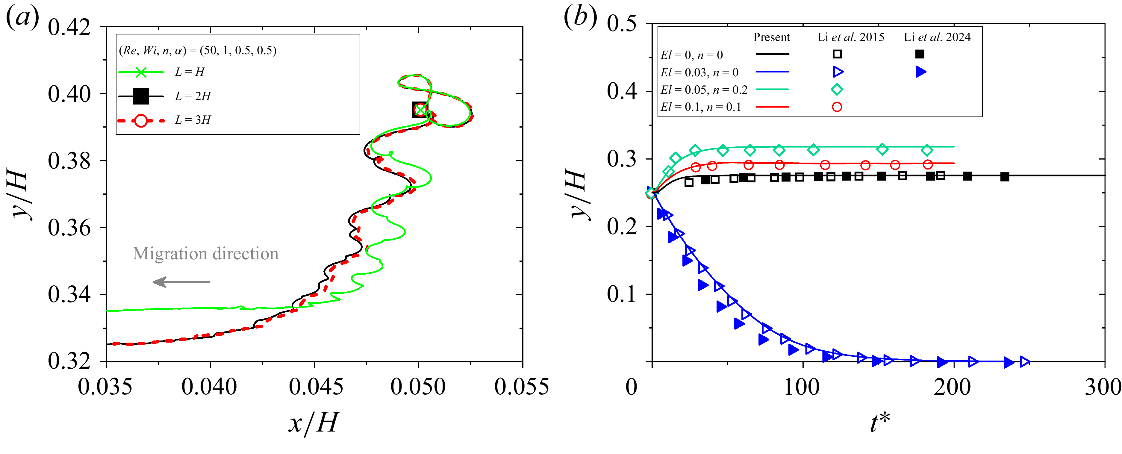
Under typical flow conditions as (Re, Wi, n, α) = (50, 1, 0.5, 0.5), the grid invariance is evaluated in figure 2(a) when the periodic length is changed as L = 128, 256 and 384. The trajectories in figure 2(a) are not changed obviously when L = 256 and 384. Thus, L = 256 is chosen in the present study. The Reynolds number is defined as Re = U 0 H/υ 0, where U 0 is the maximum fluid velocity at the channel centreline, H is the channel height and υ 0 is the viscosity (Yang, Huang & Lu Reference Yang, Huang and Lu2017). The Weissenberg number is a basic parameter in viscoelastic fluid, which is defined as Wi = λ t U 0 /H, where λ t is the fluid relaxation time (D’Avino, Del Greco & Maffettone Reference D’avino, Del Greco and Maffettone2017). The elastic number is defined as El = Wi/Re. The viscosity ratio is defined as β = η s /η 0, here 0.5 is considered. The mesh size is h = H/128, the time step is fixed at 5 × 10⁻⁴. The Courant number is defined as CFL = Um Δt/h and CFL ≈ 0.064 for Re = 100.
(a) Grid independence verification; (b) comparison of the lateral trajectory observed in the present study with those in previous works (Li et al. 2015 and Li et al. 2024).

The space-fixed coordinate system (x, y, z) and body-fixed coordinate system (x
′, y
′, z
′) for the prolate spheroid and oblate spheroid are shown in figure 1(b,c). The spheroidal particle is described as
 ${x'^{2}}/{a^{2}}+{y'^{2}}/{b^{2}}+{z'^{2}}/{c^{2}}=1$
, where a, b and c denote the lengths of three semi-axes of the particles. The aspect ratio is defined as α = c/a, where α < 1 and α > 1 correspond to the oblate spheroid (a = b) and prolate spheroid (b = c), respectively; the sphere is a special spheroidal particle with α = 1 (a = b = c). The blockage ratio of the sphere, prolate and oblate spheroids is defined as k = 2a/H, which is fixed at k = 0.2. The mesh number of the spheroidal particle has been proved to be sufficient in our previous work (Zhu et al. Reference Zhu, Yu, Pan and Shao2020). The initial particle position at the channel cross-section is denoted by (x
in
, y
in
).
The Euler angle
 $\boldsymbol{\xi}$
= (θ, φ, ψ) is defined in figure 1(b,c) in the body-fixed coordinate system;
P
denotes a unit vector along the symmetry axis of the spheroid,
P
= (P
x
, P
y
, P
z
) = (sin θ sin φ, sin θ cos φ, cos θ) can be used to determine the orientation of the spheroidal particle. The general initial orientation angle is set as
 $\boldsymbol{\xi}$
= (π/2, π/4, 0) in §§ 3.1, 3.2 and 3.3, and the effect of other initial particle orientations is studied in § 3.4.
2.2. Direct forcing/fictitious domain method
The migration of a spheroidal particle in a 3-D square duct flow of a Giesekus viscoelastic fluid is simulated using the DF/FD method, which is an efficient direct numerical simulation method. For particles migrating in a Newtonian, Oldroyd-B or Giesekus viscoelastic fluid, the present DF/FD method has been described in detail and successfully verified in our previous publications (Yu & Shao Reference Yu and Shao2007; Wang et al. Reference Wang, Yu and Lin2018; Yu et al. Reference Yu, Wang, J. and Hu2019; Hu et al. Reference Hu, Lin, Lin, Zhu and Yu2022, Reference Hu, Lin, Zhu, Yu, Lin and Li2024a ). Herein, we only briefly describe the DF/FD method as follows.
We have the continuity equation
 \begin{equation} \boldsymbol{\nabla }\boldsymbol{\cdot }\boldsymbol{u}=0 \quad \mathrm{in} \quad \mathit{\varOmega } \end{equation}
and the momentum equation
 \begin{equation} \frac{\partial \boldsymbol{u}}{\partial t}+\boldsymbol{u}\boldsymbol{\cdot }\boldsymbol{\nabla \!}\boldsymbol{u}=\frac{\mu _{r}{\nabla} ^{2}\boldsymbol{u}}{Re}-\boldsymbol{\nabla \!}p+\frac{\left(1-\mu _{r}\right)\boldsymbol{\nabla }\boldsymbol{\cdot }\boldsymbol{B}}{\textit{ReWi}}+\lambda _{p}\quad\mathrm{in} \quad \mathit{\varOmega } .\end{equation}
For the viscoelastic fluid, the Giesekus constitutive equation is used:
 \begin{equation} \frac{\partial\! \boldsymbol{B}}{\partial t}+\boldsymbol{u}\boldsymbol{\cdot }\boldsymbol{\nabla \!}\boldsymbol{B}-\boldsymbol{B}\boldsymbol{\cdot }\boldsymbol{\nabla \!}\boldsymbol{u}\boldsymbol{-}\left(\boldsymbol{\nabla \!}\boldsymbol{u}\right)^{\mathrm{T}}\boldsymbol{\cdot }\boldsymbol{B}\boldsymbol{+}\frac{n}{Wi}\left(\boldsymbol{B}-\boldsymbol{I}\right)^{2}+\frac{\boldsymbol{B}- \boldsymbol{I}}{Wi}=0\quad\text{in}\quad \mathit{\varOmega }. \end{equation}
Here u is the fluid velocity, λ p is the Lagrange multiplier that is defined in the solid domain P(t), P(t) is the solid domain, p is the pressure, μ r is the ratio of the solvent viscosity, Ω is the entire computational domain, B is the configuration tensor, τ = η p ( B − I )/λ t , and n signifies the mobility parameter to quantify the shear-thinning effect. At n = 0, we have the Oldroyd-B constitutive equation without the second normal stress difference and secondary flow. A finite-difference-based projection method is applied to a homogeneous, half-staggered grid to solve the flow equations. The Giesekus constitutive equation is calculated using the first-order time scheme and, for the convective term, a third-order upwinding MUSCL scheme is adopted in the present DF/FD method. Finally, we employ an explicit scheme to solve the equations.
In the present DF/FD method, the Newton’s equation is adopted to update particle motion:
 \begin{equation} \boldsymbol{u}=\boldsymbol{U}+\boldsymbol{\omega }_{{p}}\times \boldsymbol{r} \quad \mathrm{in} \quad P(t), \end{equation}
 \begin{equation} M\frac{\mathrm{d}\boldsymbol{U}}{\mathrm{d}t}=-\int _{P}\lambda _{p}\,\mathrm{d}\boldsymbol{s}, \end{equation}
 \begin{equation} \frac{\mathrm{d}\!\left(\boldsymbol{J}\boldsymbol{\cdot }\boldsymbol{\omega }_{{p}}\right)}{\mathrm{d}t}=-\int _{P}\boldsymbol{r}\times \lambda _{p}\,\mathrm{d}\boldsymbol{s}. \end{equation}
Here
U
and
 $\boldsymbol{\omega}$
p
denote the particle translational velocity and angular velocity,
r
is the position vector with respect to the particle mass centre,
J
is the moment of inertia tensor and d
s
is the volume element.
2.3. Validation
The present numerical method has been well validated in our previous research (Yu & Shao Reference Yu and Shao2007; Wang et al. Reference Wang, Yu and Lin2018; Hu et al. Reference Hu, Lin, Lin, Zhu and Yu2022, Reference Hu, Lin, Zhu, Yu, Lin and Li2024a ; Yu et al. Reference Yu, Wang, J. and Hu2019). Herein, we further compare the migration of a sphere in a square duct flow of a Giesekus viscoelastic fluid with the references reported by Li et al. (Reference Li, Mckinley and Ardekani2015) and Li et al. (Reference Li, Xu and Zhao2024). The blockage ratio of the sphere is fixed at k = 0.25, the initial particle position is fixed at (x in , y in ) = (0, 0.25) and the time step is 5 × 10⁻⁴, Re = 18.9. Other rheological parameters of the viscoelastic fluid are kept the same as Li et al. (Reference Li, Mckinley and Ardekani2015). As shown in figure 2(b), the particle trajectories in the Newtonian fluid, Oldroyd-B fluid and Giesekus fluid are consistent with Li et al. (Reference Li, Mckinley and Ardekani2015) and Li et al. (Reference Li, Xu and Zhao2024). Thus, it further demonstrates the accuracy of the present DF/FD method.
3. Results and discussion
The initial particle position at the channel cross-section is denoted by the purple dashed circle in figures 3, 7, 9, 11. Particles with various initial positions are released in the upper right quadrant of the square channel cross-section. When the particles reach the channel centreline, it is impossible to clearly show the distribution of the particle on the quarter channel cross-section. Thus, it has not been shown in figures 7(h), 9(e) and 11(b,e, f) when particles reached the channel centreline.
Effect of the shear-thinning on the particle trajectories on the channel cross-section with Re = 1 and Wi = 1. Results are shown for (a) n = 0, α = 0.5; (b) n = 0.25, α = 0.5; (c) n = 0.5, α = 0.5; (d) n = 0.25, α = 1; (e) n = 0, α = 2; ( f) n = 0.25, α = 2; (g) n = 0.5, α = 2; (h) n = 0.5, α = 1. The arrows on the prolate and oblate spheroids denote vectors along the symmetry axis. The sphere, prolate and oblate spheroids are represented by blue, grey and pink colours, respectively.

3.1. Effect of shear-thinning and particle aspect ratio
Taking the low fluid inertia for (Re, Wi, El) = (1, 1, 1) as an example, we first analyse the influence of shear-thinning on the migration of a spheroidal particle and then discuss the force analysis to explain the possible mechanism on particle migration.
3.1.1. Changes of the trajectories and rotational behaviours
When the distance between the spherical particle and wall does not change, as shown in figure 2(b), the stable value of y/H is defined as the equilibrium position. For the spheroidal particle, the equilibrium position is defined as the average centre of mass position attained at the final particle position along the yaxis. For better comparison, the typical particle migration behaviour in an Oldroyd-B fluid is shown in figure 3(a,e). In an Oldroyd-B fluid, only the particles close to the corner can migrate to the corner, it is named as CO equilibrium position. Particles in other initial positions can migrate to the channel centre, it is named as the CC equilibrium position. As shown in figure 3, the first normal stress difference in the centre and corner of the channel cross-section is smaller than other positions. Besides, the first normal stress difference in an Oldroyd-B fluid is significantly larger than that in a Giesekus fluid, which is decreased with increasing n.
For the oblate spheroid migrating in a Giesekus fluid at n = 0.25, as shown in figure 3(b), the oblate spheroids near the wall migrate along the wall and finally reach the CO equilibrium position. Meanwhile, oblate spheroids at other initial positions reach the CC equilibrium position. When the shear-thinning effect is enhanced ton = 0.5, as shown in figure 3(c), only oblate spheroids far from the corners migrate towards the CC equilibrium position, the oblate spheroids at other initial positions are more likely to migrate towards the CO equilibrium position. As shown in figure 3(d,h), the motion trajectory of a spherical particle on the cross-section is a smooth curve, where the migration behaviour is similar to that of the oblate spheroid.
For the prolate spheroid migrating in a Giesekus fluid at n = 0.25, as shown in figure 3( f), the prolate spheroid can reach the corner when it is close near the wall. Meanwhile, prolate spheroids at other initial positions migrate towards the CC equilibrium position. In a Giesekus fluid at n = 0.5, as shown in figure 3(g), prolate spheroids on the channel cross-section exhibit an obvious spiral motion trajectory. By comparing the area where the particle is initially released, as shown in figure 3(a–c, e–g), the area where the particles can migrate towards the CC equilibrium position is decreased with increasing n, the prolate spheroid keeps a larger area of initial position to reach the CC equilibrium position than those of oblate spheroids and spheres.
When particles reach the CC and CO equilibrium positions, the orientation of an oblate spheroid and prolate spheroid at n = 0.5 are compared at typical initial positions as an example in figure 4. In order to compare the shear-thinning effect and secondary flow in a Giesekus fluid, figure 5 shows contours of the velocity magnitude and velocity vectors when the oblate and prolate spheroids reach the CC and CO equilibrium positions.
Long-time evolution of the orientation of (a) an oblate spheroid in the kayaking, TUD and LR modes, (b) a prolate spheroid in the LR, ILR and VILR modes under different values of n and (x in , y in ), (see supplementary movie 1). The prolate and oblate spheroids are represented by grey and pink colours, respectively.

The contour of the velocity magnitude and velocity vectors when the oblate spheroids (first row) and prolate spheroids (second row) reach the equilibrium position (a) (Re, Wi, n) = (1, 1, 0.5) at the CC equilibrium position, (b) (Re, Wi, n) = (1, 1, 0.25) at the CO equilibrium position, (c) (Re, Wi, n) = (1, 1, 0.5) at the CO equilibrium position, (d) (Re, Wi, n) = (10, 1, 0.5) at the IR equilibrium position, (e) (Re, Wi, n) = (1, 1, 0.5) at the CC equilibrium position, ( f) (Re, Wi, n) = (1, 0.1, 0.5) at the CC equilibrium position, (g) (Re, Wi, n) = (1, 1, 0.5) at the CO equilibrium position, (h) (Re, Wi, n) = (10, 1, 0.5) at the IR equilibrium position. The prolate and oblate spheroids are represented by grey and pink colours, respectively.

(a) Effect of shear-thinning on the trajectories at (x in , y in ) = (0.05, 0.39). (b) Phase diagram depicting the combined effects of shear-thinning and particle aspect ratio on particle equilibrium positions. (c) The mechanism diagram of spheroidal particles with different aspect ratios affected by the velocity vectors at the CC equilibrium position and the rotational plane of the spheroidal particle.

When the particles reach the CC equilibrium position, the rotational behaviours are presented in the first row of figure 4. The prolate spheroid eventually keeps rolling around its long axis, which is referred to the LR mode. The oblate spheroid rotates like a kayak paddle moving around its equilibrium position with an amplitude, which is referred to the kayaking mode. While the rotational behaviour of the oblate spheroid in an Oldroyd-B fluid follows the LR mode, these difference can be clearly observed in supplementary movie 1 available at https://doi.org/10.1017/jfm.2026.11115. Due to the present of eight symmetric vortices in a square duct flow of a Giesekus fluid, as shown in figures 1(a) and 5(a,e, f), the velocity vectors along the DL point towards the centre of the duct, the velocity vectors near the particle will act directly on the oblate spheroid and prolate spheroid, the velocity vectors at other positions point towards the walls and corners. The velocity vectors near the particle will generate the torque for the rotation of the particles. Because the cross-sectional area of the oblate spheroid is much larger than that of the prolate spheroid, as shown in figure 6(c), the rotating oblate spheroid is more likely to be affected by the surrounding velocity vectors than the prolate spheroid. The secondary flow velocity in the duct centre is relatively small, it is not enough to make the oblate and prolate spheroids rotate completely. The oblate spheroid can only maintain kayaking rotation at the equilibrium position, while the prolate spheroid will slowly stabilise to LR mode. The opposite is true for the migration of oblate and prolate spheroids in the Oldroyd-B fluid with the same values of Wi and Re, as clearly presented in supplementary movie 1, the particles will keep the stable LR mode at the CC equilibrium position if there is no secondary flow in the Oldroyd-B fluid. Due to the small secondary flow velocity at the centre of the duct, the kayaking rotational motion of an oblate spheroid at the CC equilibrium position is extremely slower than its movement along the flow direction, which is difficult to observe experimentally.
When particles migrate to the CO equilibrium position (see the second and third rows of figure 4 for the rotational behaviours), the flow pattern in figure 5(b,c,g) becomes asymmetric. In a Giesekus fluid at high values of n, the first normal stress difference in figure 3 is reduced and the secondary flow is enhanced. The viscoelastic force in a viscoelastic fluid can be described as F
E
∼ D
r
3∇N
1(
 $\bar{\gamma}$
) (Housiadas & Tanner Reference Housiadas and Tanner2014; Davoodi et al. Reference Davoodi, Lerouge, Norouzi and Poole2018), where C
L
denotes the dimensionless lift coefficient,
 ${\gamma}$
is the shear rate, D
r
is the rotational diameter and ∇N
1 is the gradient of the first normal stress difference and
 $\bar{\gamma}$
is the average shear rate. Therefore, the viscoelastic force is reduced with increasing n. The enhanced secondary flow will attract the particle to follow the direction of the velocity vectors, and the obvious spiral motion trajectory is observed in figure 3(c,g). As shown in figure 5(b,c), the oblate spheroids at the CO equilibrium position induce the large velocity vectors that point towards the centre of the duct, and the velocity vectors induced by the Giesekus fluid act on the particle surface. As shown in figure 5(g), the prolate spheroids at the CO equilibrium position induce the large fluid velocity at two ends of the long axis, and the induced particle migration velocity is much smaller than that of the oblate spheroid in figure 5(c). Due to the asymmetric flow field, the two unequal velocity vectors and the wall lift force generate torque and promote the rotation of particles. Specifically, the oblate spheroid keeps the large rotational diameter at the CO equilibrium position and maintains tumbling on the diagonal plane with a large rotational amplitude, which is referred to the TUD mode. The prolate spheroid keeps the small rotational diameter at the CO equilibrium position, maintains rolling around its long axis with a small rotational amplitude, and finally, maintains the orientation inclined to the DL of the square duct, which is referred to the ILR mode. In an Oldroyd-B fluid, the oblate spheroid (third row of figure 4
a) keeps the LR mode near the wall. The prolate spheroid in an Oldroyd-B fluid also rotates as in the ILR mode with a small rotational amplitude along the long axis, which is referred to the VILR mode.
Taking the typical initial particle position at (x in , y in ) = (0.05, 0.39) as an example, we further analyse the influence of the shear-thinning property on the equilibrium positions and the streamwise travel distance for the particles to reach the final equilibrium position. As shown in figure 6(a), the prolate spheroid and oblate spheroid all migrate to the CO equilibrium position when the shear-thinning effect is strong. Only when the shear-thinning is small can the particles in figure 6(a) migrate to the CC equilibrium position as in the Oldroyd-B fluid. For spheroidal particles with different aspect ratios and shear-thinning effects at (x in , y in ) = (0.05, 0.39) for (Re, Wi) = (1, 1), the phase diagram in figure 6(b) shows whether the spheroidal particles can migrate to the CC equilibrium position at different values of n and α. Because the cross-sectional area of the oblate spheroid is much larger than that of the prolate spheroid, as shown in figures 5(a,e) and 6(c), the oblate spheroid keeps the larger rotational diameter by the enhanced torque, which is produced by the velocity vectors near the particle; the oblate spheroid is more susceptible to the velocity vectors of the secondary flow than the prolate spheroid. The oblate spheroid will be more likely to deviate from the CC equilibrium position and migrates towards the wall and corner than the prolate spheroid. Due to the fact that the cross-sectional area of the prolate spheroid is decreased with increasing α, as shown in figure 6(c), the cross-sectional area in which the velocity vectors act on the spheroid is decreased with increasing α. The prolate spheroid with the slender shape can keep the CC equilibrium position under a relatively stronger shear-thinning effect. This inspires us to show that the spheroidal particles with different shapes can be efficiently separated via the shear-thinning effect of a Giesekus fluid. The possible fluid mechanism of different motion phenomena of particles in Oldroyd-B and Giesekus viscoelastic fluids will be described in detail in the next section.
3.1.2. Force analysis
In this section we attempt to determine the type of forces mainly responsible for particle migration under different shear-thinning effects and particle shapes and the contribution of these forces on the surface of the particles are considered in this section. The adopted FD method is a non-boundary-fitted approach, and the interpolation technique is adopted to calculate the stress on the particle surface.
In order to explain the mechanism of why particles migrate towards the centre of the duct or the wall, the particle position in this section is maintained in the x–y cross-plane with an initial lateral position fixed at (x in , y in ) = (0, 0.25); the particles can move along the flow direction and rotate. The total hydrodynamic force in the y direction (F y ) can be disintegrated into three main parts: pressure F p , viscous F V and polymer F E forces, which can be calculated as follows:
 \begin{equation} F_{p}=\int _{\partial P}-n_{y}p {\rm d}S, \end{equation}
 \begin{equation} F_{V}=\eta _{s}\int _{\partial P}\left[2n_{y}\frac{\partial u_{y}}{\partial y}+n_{x}\!\left(\frac{\partial u_{y}}{\partial x}+\frac{\partial u_{x}}{\partial y}\right)+n_{z}\!\left(\frac{\partial u_{y}}{\partial z}+\frac{\partial u_{z}}{\partial y}\right)\right]{\rm d}S, \end{equation}
 \begin{equation} F_{E}=\int _{\partial P}\left(n_{x}\tau _\textit{xy}+n_{y}\tau _\textit{yy}+n_{z}\tau _\textit{yz}\right){\rm d}S. \end{equation}
The polymer force (F E ) can be further decomposed into the polymer normal force (F En ) and the polymer shear force (F Es ):
 \begin{equation} F_\textit{En}=\int _{\partial P}n_{y}\tau _\textit{yy}\,{\rm d}S, \end{equation}
 \begin{equation} F_\textit{Es}=\int _{\partial P}\left(n_{x}\tau _\textit{xy}+n_{z}\tau _\textit{yz}\right){\rm d}S .\end{equation}
The pressure force in (3.1) is calculated from the pressure to satisfy the incompressibility constraint. In a viscoelastic fluid the polymer isotropic stress (τ xx + τ yy + τ zz )/3 or the average polymer normal stresses can also be regarded as ‘pressure’, and the elasticity-induced force is related to the normal stress differences (Ho & Leal Reference Ho and Leal1976). Therefore, the polymer normal force (F En ) can be decomposed into the polymer ‘pressure’ force (F Enp ), the force from the first normal stress difference (F En1) and the second normal stress difference (F En2):
 \begin{equation} F_\textit{En}=\underset{F_{Enp}}{\underbrace{\int _{\partial P}n_{y}\frac{\tau _{xx}+\tau _\textit{yy}+\tau _\textit{zz}}{3}{\rm d}S}}+\underset{F_{En1}}{\underbrace{\int _{\partial P}n_{y}\frac{\tau _\textit{yy}-\tau _\textit{zz}}{3}{\rm d}S}}+\underset{F_{En2}}{\underbrace{\int _{\partial P}n_{y}\frac{\tau _\textit{yy}-\tau _{xx}}{3}{\rm d}S}} .\end{equation}
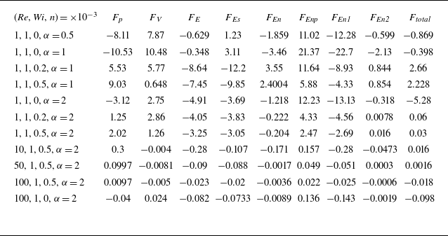
The force analysis on the particle with a fixed lateral position at steady state for some typical cases are presented in table 1. When (Re, Wi) = (1, 1), it can be seen from table 1 that the pressure force, as opposed to the viscous force or polymer force, is the most important driving force for particle migration. Due to the shear-thinning effect of the Giesekus fluid, the viscous force on particles in an Oldroyd-B fluid is greater than that in a Giesekus fluid. In an Oldroyd-B fluid, the pressure force on particles points to the negative direction of the yaxis, the force direction of F p and F Enp is opposite, and the force from the first normal stress difference (F En1) becomes the driving force for the cross-stream migration, consistent with the theory of Ho & Leal (Reference Ho and Leal1976). Therefore, under the action of pressure force (F p and F Enp ) and F En1, particles in an Oldroyd-B fluid mainly migrate to the low first normal stress region at the duct centre. In a Giesekus fluid, the action of F En1 weakens and the pressure force on particles points to the positive direction of the yaxis, i.e. the walls of the duct. When the forces of F p and F Enp keep the same direction, the pressure force (F p and F Enp ) is the main force to push the particles towards the walls, resulting in a different trajectory from that in an Oldroyd-B fluid. At the same values of Re and Wi, the pressure force on a spherical particle is the largest, then followed by the oblate spheroid and the prolate spheroid is the smallest. Therefore, the prolate spheroid in figure 6(a) can migrate to the centre of the duct under the higher shear-thinning by the reduced pressure force. As the shear-thinning effect in a Giesekus fluid increases, the pressure force on particles gradually increases, and the corresponding travel distance in figure 6(a) is decreased with increasing n. The first normal stress difference (F En1) of particles in an Oldroyd-B fluid is greater than that in a Giesekus fluid, which is consistent with the result in figure 3 that the first normal stress difference decreases with increasing n. Therefore, with the increase of the shear-thinning effect, the area of the initial particle position where particles can migrate to the CC equilibrium position is decreased. The second normal stress difference (F En1) is enhanced in a Giesekus fluid by increasing n and the secondary flow intensity is enhanced.
Effects of shear-thinning and particle shape on the forces on the particle with a fixed lateral position (
 $x_0$
,
 $y_0$
) = (0, 0.2), the forces are normalised by
 $\eta_{0}U_{0}H$
. Here F
p
, FV
, F
E
, FEs
, FEn
, FEnp
, FEn
1 and FEn
2 represent the pressure force, viscous force, polymer force, polymer shear force, polymer normal force, polymer pressure force and the first and second normal stress difference forces defined in (3.1)–(3.6), respectively.

Whilst this section focused mainly on the forces at (Re, Wi) = (1, 1), force analysis at larger Reynolds number (see table 1) are compared in the next section when analysing the elastic effect.
Effect of the elastic number on the particle trajectories when (Re, Wi, α) equals (a) (0.25, 1, 0.5), (b) (0.25, 1, 1), (c) (5, 1, 0.5), (d) (1, 0.1, 0.5), (e) (0.25, 1, 2), ( f) (0.5, 1, 2), (g) (5, 1, 2), (h) (1, 0.1, 2). The sphere, prolate and oblate spheroids are represented by blue, grey and pink colours, respectively.

3.2. Effect of elastic number on the migration behaviour and the induced secondary flow
The elastic number can be used to characterise the relative magnitude of the elasticity and inertia of a viscoelastic fluid. Therefore, the influence of elastic number on the motion and rotational behaviours of an oblate spheroid (α = 0.5), sphere (α = 1) and prolate spheroid (α = 2) are further studied. This section mainly focuses on the migration behaviours of particles in a Giesekus fluid at n = 0.5, the typical flow parameters are selected as 0.25 ≤ Re ≤ 100 and 0 ≤ Wi ≤ 1.
3.2.1. When the fluid inertia is low with Re ≤ 5
When fluid inertia is negligible, taking (Re, Wi, n) = (0.25, 1, 0.5) as an example, the motion trajectories of an oblate spheroid, sphere and prolate spheroid at different initial positions are shown in figure 7(a,b,e). Particles far from (close to) the channel centre migrate to the CO (CC) equilibrium positions, as shown in figures 4 and 8, the oblate spheroid and prolate spheroid keep the TUD and ILR (kayaking and LR) modes, with the oblate spheroid keeping a larger rotational diameter than the prolate spheroid. The results of spherical particles in figure 7(b) are basically consistent with the migration behaviours shown in figure 3(h). Prolate spheroids in figure 7(e) can form the spiral trajectory on the channel cross-section, which is considerably different from that shown in figure 3(g). The half-quadrant of the square channel cross-section can be divided into three regions: the CC-attractive, the CO-attractive and the spiral rotating zones. Although the oblate spheroid in figure 7(a) tends to maintain the spiral trajectory, the spiral trajectory is not as obvious as that of the prolate spheroid. Under the Stokes flow condition (Re ≈ 0), Villone et al. (Reference Villone, D’avino, Hulsen, Greco and Maffettone2013) reported that some spherical particles could form the spiralling trajectory, and this phenomenon disappeared by increasing the diameter of spherical particles. It is consistent with the present results that the prolate spheroid keeps a smaller rotational diameter than the oblate spheroid, as it is easier to form a spiral trajectory.
When (Re, Wi, n) = (0.5, 1, 0.5), taking the prolate spheroid in figure 7( f) as an example, a tendency for a spiral trajectory is also observed. When the Reynolds number is increased to 5, the prolate spheroids in figure 7(g) show the obvious spiral trajectory again. When the spiral trajectory approaches the corner, the prolate spheroid migrates to the CO equilibrium position. In addition, as shown in figures 3(g) and 7(e–g), the distance between the prolate spheroid and the wall is decreased with increasing Re. It is difficult for the prolate spheroid to keep the stable ILR mode at the CO equilibrium position due to the enhanced wall-induced lift force acting on it. Thus, as shown in the third row of figure 8(b), the prolate spheroids keep the ILR mode with a small rotational amplitude along the long axis (VILR mode). By comparing figure 7( f) with figure 3(g), which is associated with a closed Reynolds number, the area from which the prolate spheroid can migrate to the stable CO equilibrium position increases when Re = 0.5 ∼ 5. The oblate spheroids in figure 7(c) cannot exhibit the spiral trajectory. In the third row of figure 8(a), the oblate spheroids keep the TUD mode; however, the curves of P x and P y do not overlap, which is slightly different from that at Re = 0.25 ∼ 1. This rotational mode will be discussed in detail in § 3.4. Besides, the area of the initial particle position where oblate spheroids can migrate to the CO equilibrium position remains almost unchanged when Re ≤ 5. Due to the fact that the migration velocity scales as V M ∼ Dr 2 Wi (D’Avino et al. Reference D’avino, Romeo, Villone, Greco, Netti and Maffettone2012), the oblate spheroid maintains a large migration velocity and so can always overcome the influence of secondary flow and migrate to the wall when Re ≤ 5.
When Wi = 0.1, compare figures 7(d,h) and 3(c,g–h) at the same values of Re and n, the first normal stress difference on the channel cross-section is significantly decreased as Wi decreases. As shown in figure 5(e–f), the induced secondary flow in figure 5( f) is significantly reduced, which is consistent with the theory of Yue et al. (Reference Yue, Dooley and Feng2008) as V SF ∼ Wi 4. Only the relative large velocity is generated near the particles, although the shear-thinning property remains the same as figure 5(e). Due to the reduced effect of secondary flow, the CO equilibrium position appears when an oblate spheroid is close to the corner, which is similar to the migration of an oblate spheroid in the Oldroyd-B fluid in figure 3(a).
Long-time evolution of particle orientation: (a) the oblate spheroids all keep the TUD mode under different flow conditions, (b) from the top to bottom, the prolate spheroid changes from the ILR, ILR and VILR modes. The prolate and oblate spheroids are represented by grey and pink colours, respectively.

Effect of the elastic number on particle trajectories when n = 0.5, and (Re, Wi, α) equals (a) (10, 0.1, 0.5), (b) (10, 1, 0.5), (c) (20, 1, 0.5), (d) (30, 1, 0.5), (e) (10, 0.1, 2), ( f) (10, 1, 2), (g) (10, 1, 1), (h) (30, 1, 2). The sphere, prolate and oblate spheroids are represented by blue, grey and pink colours, respectively.

3.2.2. When fluid inertia is moderate with Re = 10–30
By increasing the fluid inertia for Re = 10–30, we can further analyse the competition between the influences of fluid inertia and elastic effects on the migration of particles.
When (Re, Wi, n) = (10, 0.1, 0.5), as shown in figure 9(a,e) and the first row of figure 10, there are no CO equilibrium positions for both oblate and prolate spheroids. Oblate spheroids keep the TUD mode and stabilise at the DL of the square duct, which is referred to the DL equilibrium position. While a prolate spheroid can migrate towards the duct centre along the DL, it rotates like a kayak paddle with a small amplitude for an extremely long time, as shown in the first row of figure 10(b).
Long-time evolution of the particle orientation: (a) the oblate spheroid keeps the TUD, TUD and kayaking modes; (b) the prolate spheroid keeps the kayaking, ILR and kayaking modes. The prolate and oblate spheroids are represented by grey and pink colours, respectively.

When (Re, Wi, n) = (10, 1, 0.5), most of the oblate and prolate spheroids in figure 9(b, f) exhibit obvious spiral trajectories and eventually focus at a new equilibrium position near the wall, the TUD mode and ILR mode are observed in the second row of figure 10, respectively. Under the Stokes flow condition (Re ≈ 0), Villone et al. (Reference Villone, D’avino, Hulsen, Greco and Maffettone2013) reported that some spherical particles could form the spiralling trajectory on the channel cross-section, but most of their particles could not focus on this spiralling trajectory. When the fluid inertia is relatively strong, the present new equilibrium position is different with the observation of Villone et al. (Reference Villone, D’avino, Hulsen, Greco and Maffettone2013), and we define it as the IR equilibrium position. The formation of the IR equilibrium position depends mainly on the migration velocity of the particles and the secondary flow velocity in a Giesekus fluid. With increasing Re, as shown in figure 5(c,d,g,h), the velocity vectors induced by particles increase and the particles migrate towards the wall bisector. This is due to the fact that the particles are also affected by the secondary flow velocity vectors, which point away from the wall bisector. By the interaction of two kinds of velocity vectors, the particles are finally stabilised at the IR equilibrium position near the wall bisector. More importantly, the IR, CC and CO equilibriums coexist simultaneously in figure 9(b, f). As shown in figures 3(c,g), 7(c,g) and 9(b–d, f,h), the area of the initial particle position where oblate and prolate spheroids can migrate to the CC and CO equilibrium positions decreases as the fluid inertia increases. The spherical particle does not have the rotational motion behaviour, as shown in figures 13(b,e,g) and 14, it keeps the larger migration velocity than the oblate spheroid and prolate spheroid. The spherical particles at most initial positions with a large migration velocity overcome the effect of secondary flow and migrate towards the CSM equilibrium position, and the spiralling trajectory and IR equilibrium position is not observed in figure 9(g). Only the spherical particles very close to the corners (channel centre) can stabilise at the CO (CC) equilibrium position. As confirmed in table 1, the pressure force facing towards the wall in a Giesekus fluid is decreased with increasing Re; thus, the area where particles can migrate to the corner also decreases. In an Oldroyd-B fluid at the same elastic number (Hu et al. Reference Hu, Lin, Zhu, Yu, Lin and Li2024a ), the particles are always subjected to pressure forces directed to the centre of the duct, and there is no IR and CSM equilibrium positions, which is a considerably different phenomenon.
Effect of the elastic number on particle trajectories when (Re, Wi, α) equals (a) (50, 0.1, 0.5), (b) (50, 1, 0.5), (c) (100, 1, 0.5), (d) (50, 0.1, 2), (e) (50, 1, 2), 1, ( f) (100, 1, 2). The trajectories of particles in a Giesekus fluid (n = 0.5) and an Oldroyd-B fluid (n = 0) are depicted at the upper and lower half-quarters of the channel cross-section, respectively. The prolate and oblate spheroids are represented by grey and pink colours, respectively.

When the Reynolds number is further increased to (Re, Wi, n) = (20, 1, 0.5), the migration behaviour changes. Taking figure 9(c) as an example, the CC and CO equilibrium positions are not found for the migration of an oblate spheroid, and the IR equilibrium position becomes obvious. When (Re, Wi) = (30, 1), oblate spheroids in figure 9(d) migrate to the CSM equilibrium position. On the contrary, the prolate spheroids still maintain CC and IR equilibrium positions in figure 9(h) when (Re, Wi) = (30, 1), the CO equilibrium position is not found. When Re is increased from 10 to 30, as shown in the second and third rows of figure 10(a,b) at Wi = 1, the oblate (prolate) spheroids transition to the TUD and kayaking modes (ILR and kayaking modes), and the oblate spheroid always keeps a larger rotational diameter than the prolate spheroid. Due to the fact that the migration velocity is increased with increasing rotational diameter, i.e. V M ∼ Dr 2 Wi (D’Avino et al. Reference D’avino, Romeo, Villone, Greco, Netti and Maffettone2012), the oblate spheroid with a larger migration velocity is closer to the wall bisector and migrates earlier towards the CSM equilibrium position than the prolate spheroid. With increasing Re, as shown in figure 10(b–d, f,h), the prolate spheroid keeps a smaller migration velocity than the oblate spheroid, which is more susceptible to the secondary flow and maintains the IR equilibrium position.
3.2.3. When the fluid inertia is obvious with Re = 50–100
By further increasing the Reynolds number, the fluid inertial effect becomes pronounced. For a better comparison, the trajectories of particles in a Giesekus and Oldroyd-B fluid are simultaneously presented in figure 11. As shown in figure 11, there are no CC and CO equilibrium positions, the particles all migrate away from the channel centreline and corner, independent of their initial positions.
When (Re, Wi, n) = (50, 0.1, 0.5), the fluid inertia dominates while the elastic effect and the first normal stress difference is relatively weak. As shown in figure 11(a,d) and the second row of figure 12, the oblate and prolate spheroids migrate towards the DL equilibrium position with ILR and TUD modes, respectively. The particle migration behaviours in a Giesekus fluid are similar to those in an Oldroyd-B fluid when the elastic number is small. In other words, the shear-thinning effect on the particle trajectory is not obvious when the elastic number is small. This conclusion is further confirmed by the result in the first row of figure 12 with negligible elasticity. The oblate and prolate spheroids reach the CSM equilibrium position and maintain the LR and TU modes, which is consistent with the rotational modes in inelastic power-law fluids (Hu et al. Reference Hu, Kang, Lin, Lin, Bao and Zhu2023).
Long-time evolution of particle orientation: (a) the oblate spheroid keeps the LR, ILR and LR modes; (b) the prolate spheroid keeps the TU, TUD and kayaking modes. The prolate and oblate spheroids are represented by grey and pink colours, respectively.

When (Re, Wi, n) = (50, 1, 0.5), as shown in figure 11(b,e) and the third row of figure 12, the oblate spheroid and prolate spheroid in a Giesekus fluid migrate to the CSM equilibrium position in the LR mode and kayaking mode, respectively. On the contrary, both prolate and oblate spheroids in an Oldroyd-B fluid still migrate to the CC equilibrium position at (Re, Wi, n) = (50, 1, 0). When (Re, Wi, n) = (100, 1, 0.5), as shown in figure 11(c, f), oblate and prolate spheroids in a Giesekus fluid migrate to the CSM equilibrium positions. In an Oldroyd-B fluid with (Re, Wi, n) = (100, 1, 0), the oblate spheroids migrate to the DL equilibrium position, while prolate spheroids can still stabilise at the CC equilibrium position.
The changes of the migration behaviour can be explained by the rotational mode at different Reynolds numbers. Firstly, taking the prolate spheroid in table 1 as an example, although the absolute value of the pressure force on the particles in a Giesekus and Oldroyd-B fluid is decreased with increasing Re, the force direction is different. In an Oldroyd-B (Giesekus) fluid, the pressure force remains as a negative (positive) value, and the particles can migrate to the duct centre (wall). Secondly, as shown in the second and third rows of figure 10 and the third row of figure 12, the oblate spheroids keep the LR mode with a larger rotational diameter at higher Re. The variation range of the orientation of prolate spheroids is enhanced with increasing Reand the prolate spheroid keeps the kayaking mode with a small rotational diameter. For these two reasons, the oblate spheroids induce a higher migration velocity to overcome the elastic effect and migrate to the equilibrium position of the CSM earlier than the prolate spheroids. A larger Reynolds number is needed for the prolate spheroid to change from the IR equilibrium position to the CSM equilibrium position.
Effect of the elastic number on the y-component velocity contours and the streamlines on the cross-section when particles reach the final equilibrium position, n = 0.5 and (Re, Wi, α) equals (a) (10, 1, 0.5) at the CO equilibrium position, (b) (10, 1, 0.5) at the IR equilibrium position, (c) (50, 1, 0.5) at the CSM equilibrium position, (d) (10, 1, 1) at the CSM equilibrium position, (e) (10, 1, 2) at the CO equilibrium position, ( f) (10, 1, 2) at the IR equilibrium position, (g) (50, 1, 2) at the CSM equilibrium position, (h) (50, 1, 1) at the CSM equilibrium position. Notably, when spheroids experience the TUD and kayaking motion, the flow field and streamlines can be different depending on the instantaneous particle orientation. The sphere, prolate and oblate spheroids are represented by blue, grey and pink colours, respectively.

Averaged secondary flow velocity when a particle reaches the CO, DL equilibrium positions (first line) or the CC, IR and CSM equilibrium positions (second line). Results are shown for (a,d) α = 0.5, (b,e) α = 1, (c, f) α = 2.

3.2.4. Changes of the induced secondary flow
By varying the elastic numbers and initial particle positions, the induced secondary flow velocity is further analysed at different equilibrium positions. When the particles reach the CO, IR, CSM and DL equilibrium positions, figure 13 presents the contour of the lateral velocity at the vertical cutting plane at different Reynolds numbers. In order to quantitatively compare the secondary flow velocity when the particle reaches the CO and DL equilibrium positions or the CC, CSM and IR equilibrium positions, the averaged secondary flow velocity
 $\langle u_{y}\rangle _{z,y}$
in the z and y directions are analysed in figure 14(a–c) and figure 14(d–f), respectively. The y component of flow velocity is numerically integrated in the region ± 0.75 upstream and downstream of the spheroidal particle in the streamwise (z) direction and the integration is performed in the entire domain [−0.5, 0.5] in the y direction:
 \begin{align} \left\langle u_{y}\right\rangle _{z,y}=\frac{1}{A_\textit{zy}}\int _{-0.5}^{0.5}\int _{-0.75}^{0.75}u_{y}\,{\rm d}y \, {\rm d}z\cong \frac{1}{\left(z_\textit{max}-z_\textit{min}+1\right)N_{y}}\sum _{j=1}^{N_{y}}\sum _{z=z_\textit{min}}^{z_\textit{max}}\left(u_{y}\right)_{jk}. \end{align}
Here A zy is the area of the ZOY plane, z min = (z p −0.75)N z /L and z max = (z p + 0.75)N z /L, where z p is the particle position and N y and N z the number of grid points in the y and z directions, respectively.
If the particle migrates towards the CO equilibrium position, as shown in figures 5(b,c,g) and 13(a,e), their presence can affect the induced vortices at this corner position, with stable vortices still observed at the other three corners. Thus, the secondary flow induced near the particle is enhanced, the curves of the averaged secondary flow velocity in figure 14(a–c) becomes asymmetric. For the particles at the CC equilibrium position, the symmetric vortices are observed in figure 5(a,e, f), and the averaged secondary flow velocity in figure 14(d–f) remains negligible when Re is small. When Re = 10, 20, the oblate spheroid and prolate spheroid keep the IR equilibrium position, the averaged secondary flows are asymmetric, as shown in figures 5(d,h), 13(b, f) and 14(d, f). In figure 14, an increase in the fluid inertia increases the averaged secondary flow velocity. Upon further increasing the Reynolds number, taking Re = 50 in figures 13(c,g,h) and 14(d–f) as examples, the induced secondary flow velocity is further increased with increasing Re. Consequently, the particles in a Giesekus fluid in figures 9(c,d,g,h) and 11 move away from the CC and CO equilibrium positions. When particles reach the CSM equilibrium position, due to the symmetric shape of spheres and oblate spheroids in the LR mode, the averaged secondary flow velocity in figure 14(d–f) shows two peaks and remains symmetric. On the contrary, the prolate spheroids at the CSM equilibrium position keep the kayaking mode, its rotational behaviour leads to an asymmetric secondary flow velocity.
All in all, the spherical particles induce the largest secondary flow velocity, then followed by the oblate spheroids and the prolate spheroids always induce the smallest velocity, consistent with the results in the above sections. This further explains why spheres and oblate spheroids migrate earlier towards the CSM equilibrium position than prolate spheroids as the Reynolds number is increased.
3.3. Changes of the equilibrium positions
The equilibrium position identified in §§ 3.1 and 3.2 are complex, including the CC, CO, IR, DL, CSM equilibrium positions. This section will further compare the effect of El and Re on the changes in the equilibrium positions of spheroidal particles. Because the elastic number is simultaneously influenced by Re and Wi, the effects of these two factors are analysed separately.
The effect of Wi on the equilibrium position is first evaluated by keeping the Reynolds number fixed and setting the initial particle position as (x in , y in ) = (0.39, 0.39). When Re = 1, as shown in the first row of figure 15(a), the oblate and prolate spheroids can all migrate to the CC equilibrium position at a low elastic number. As shown in figures 3(c,g) and 4, the oblate spheroids keep the large rotational diameter (TUD mode) will reach the CO equilibrium position earlier than the prolate spheroid, who keeps the LR mode with small rotational diameter. At the CO equilibrium position, the change in the equilibrium position with El is not obvious, and prolate spheroids are closer to the wall than oblate spheroids. When Wi is increased and Re is fixed at 10, the equilibrium position in the second row of figure 15(a) first decreases, then increases rapidly and finally stabilises at the CO equilibrium position. When Re = 50, similar changes in the equilibrium position are observed in the third row of figure 15(a), but the oblate and prolate spheroids keep the CSM equilibrium position rather than the CO equilibrium position, as shown in figure 11(b,c,e, f). When Re = 1, 10 and 50, there is a critical elastic number where the particle equilibrium position in a Giesekus fluid rapidly increases with increasing elastic number. It is interesting to note that the larger the Reynolds number, the lower the elastic number for the rapid transition of the particle equilibrium position. The main reason is the enhanced secondary flow caused by increasing Wi. When Re is small, as shown in table 1 and figure 5(a,b,e, f), the migration velocity of the particles is small and the secondary flow of the Giesekus fluid is large. The particle is subject to the secondary flow and can migrate to the wall and corner, and the equilibrium position increases. With increasing Re, as shown in table 1, the effect of positive pressure force and the first normal stress difference on the particles decreases, the relative influence of the secondary flow and fluid inertia increases, which is confirmed by the enhanced secondary flow in figures 13 and 14. When the value of Wi is small, as shown in figure 5( f), the effect of the secondary flow is weak. Taking Re = 50 as an example, the inertia acting on the particles dominates, and the particles migrate to the DL equilibrium position. When Wi = 0.2, the elastic force acting on the particles increases. The DL equilibrium position of the particles approaches the duct centre, the equilibrium position decreases initially. When Wi = 0.5, similar to figure 5(e, f), the secondary flow in a Giesekus fluid is enhanced. Since the velocity vectors of the secondary flow are directed from the duct centre towards the wall, the particle induced velocity also increases under high fluid inertia. Under the action of the secondary flow and the particle induced velocity, inertia dominates. The particles migrate towards the CSM equilibrium position and the equilibrium position increases. The secondary flow is not observed in an Oldroyd-B fluid, the particle will reach the CC equilibrium position at a high elastic number, and the equilibrium position decreases rapidly with increasing El (Hu et al. Reference Hu, Lin, Zhu, Yu, Lin and Li2024a ). Therefore, in Oldroyd-B and Giesekus fluids the equilibrium position of particles shows the opposite trend with the change of elastic number.
Changes in the final particle equilibrium position. (a) Effect of the elastic number at Re = 1, 10, 50; (b) effect of Re at Wi = 1. The grey, pink, green and orange areas represent the CC, CO, IR and CSM equilibrium positions, respectively.

When Wi = 1, whether the spheroidal particles can keep the stable CC and CO equilibrium positions are further analysed across different Reynolds numbers. The results are shown in figure 15(b), two typical initial particle positions, (x in , y in ) = (0.39, 0.39) and (x in , y in ) = (0.025, 0.05), are selected. When (x in , y in ) = (0.39, 0.39) and Re ≤ 10, both oblate and prolate spheroids have CO equilibrium positions, and the equilibrium positions shift closer to the wall with increasing Re. When the Reynolds number is further increased, the oblate and prolate spheroids move away from the CO equilibrium position, the equilibrium position rapidly decreases, and the IR and CSM equilibrium positions gradually appear. When the particles are released near the channel centre at (x in , y in ) = (0.025, 0.05), the oblate (prolate) spheroids can migrate to the CC equilibrium position at Re ≤ 10 (Re ≤ 30). As the Reynolds number is further increased, the equilibrium position is increased suddenly, the IR and CSM equilibrium positions are also observed. Thereafter, the final equilibrium positions of the spheroidal particles at the two initial positions are equal, the prolate spheroid with a smaller rotational amplitude is always closer to the wall than the oblate spheroid.
Phase diagrams for the equilibrium positions of (a) the oblate spheroid for α = 0.5 and (b) the prolate spheroid for α = 2 when
 $n = 0.5$
and
 $0.01 \leq Wi \leq 1$
. The ability of oblate and prolate spheroids to maintain the CC equilibrium position can be divided by the empirical formulas as Wi = 0.055 Re–0.1 and Wi = 0.045 Re–0.35.

Based on the changes of the equilibrium position, the relationships among the equilibrium positions, Re and Wi are further compared in the phase diagram in figure 16. The spheroidal particles in a Giesekus fluid at high Wi and low Re simultaneously have two or more equilibrium positions. When the elasticity dominates, the oblate spheroid and prolate spheroid can maintain the CC, CO and IR equilibrium positions simultaneously. As the Reynolds number is increased, the number of equilibrium positions decreases, and the particles mainly maintain the CSM or DL equilibrium position. An interesting finding is that the ability of oblate and prolate spheroids to maintain a stable CC equilibrium position can be divided by the empirical formulas as Wi ∼ 0.055 Re−0.1 and Wi ∼ 0.045 Re−0.35, respectively. Specifically, the stable CC equilibrium position can be formed to the left of the lines in figure 16 and vice versa. The slopes of these lines can be considered as the critical elastic number for the migration of spheroids in a Giesekus fluid, i.e. El c = 0.055 and 0.045 for the oblate and prolate spheroids, respectively. The critical elastic number for the migration of a sphere, oblate and prolate spheroids, atk = 0.2, in an Oldroyd-B fluid is approximately 0.0152 (Hu et al. Reference Hu, Lin, Zhu, Yu, Lin and Li2024a ; Yu et al. Reference Yu, Wang, J. and Hu2019; Li et al. Reference Li, Xu and Zhao2024). Because of the secondary flow effect, the critical elastic number in a Giesekus fluid is significantly higher than that in an Oldroyd-B fluid. As shown in figures 7 and 9, particles in Giesekus fluids exhibit rich equilibrium positions even when the fluid inertia is relatively small. Controlling the fluid elasticity can reduce the number of equilibrium positions and result in the efficient separation of particles in Giesekus fluids.
3.4. Initial orientation affects the migration behaviour near the critical elastic number
For the aforementioned general initial particle positions in figures 3, 7, 9 and 11, the effect of the initial orientation of spheroidal particles on their final equilibrium position is negligible. Therefore, we further analyse whether the initial orientation angle affects the final equilibrium position and rotational mode by initially placing the particles at two special positions, i.e. at the corner (x
in
, y
in
) = (0.39,0.39) and wall bisector (x
in
, y
in
) = (0, 0.39). Due to the large number of calculation parameters and complex migration phenomenon, this section selects the typical working condition as (Wi, n) = (1, 0.5). The Reynolds numbers is varied as Re = 1, 5, 10, 20, 30, 50 and 100. Typical initial Euler angles are chosen as
 $\boldsymbol{\xi}$
= (π/2, π/2, 0), (0, 0, 0), (π/2, 0, 0), (π/4, π/4, 0) and (π/2, π/4, 0). Finally, the phase diagram of an oblate spheroid and a prolate spheroid is obtained in figure 17.
Phase diagram of the rotational behaviours for an oblate spheroid with α = 0.5 (pink half-circle) and a prolate spheroid with α = 2 (grey half-circle). At (Wi, n) = (1, 0.5), the Reynolds numbers are varied from the inner circle to the outer circle as Re = 100, 50, 30, 20, 10, 5 and 1, respectively.

The phase diagram reveals that the rotational mode of the oblate spheroid is mainly affected by the elastic number, and that the initial orientation does not affect the rotational mode when the oblate spheroid is initially placed near the corner. As the elastic number decreases, initially, oblate spheroids at the corner and wall bisector successively exhibit the TUD, kayaking and LR modes. Only when
 $\boldsymbol{\xi}$
= (0, 0, 0) and (π/2, 0, 0), the oblate spheroid at the wall bisector can maintain the tumbling (TU) mode. When Re ≥ 20, the prolate spheroid cannot maintain the stable CO equilibrium position, it will migrate towards the IR equilibrium position in the kayaking mode, the initial orientation has no effect on the final rotational mode. When Re ≤ 5 and (x
in
, y
in
) = (0.39, 0.39), the prolate spheroids at
 $\boldsymbol{\xi}$
= (0, 0, 0) or (π/2, 0, 0) maintain the TUD mode, while those with other initial orientations maintain the ILR and VILR modes at Re = 1 and Re = 5, respectively. Only when the fluid inertia is small (Re ≤ 10) does the initial orientation affect the final rotational mode when the prolate spheroid maintains the stable CO equilibrium position; a detailed analysis is given below.
For an oblate spheroid with small fluid inertia (Re = 1), as shown in the second row of figure 4(a) and the first row of figure 18(a), an oblate spheroid at the CO equilibrium position can maintain the stable TUD mode. Although the initial trajectory of the oblate spheroid in figure 18(a) oscillates, it eventually stabilises on the DL. When Re = 5 ∼ 10, taking Re = 10 in the second row of figure 18(c) as an example, the curves of P
x
and P
y
no longer overlap when
 $\boldsymbol{\xi}$
= (π/4, π/4, 0). Only when
 $\boldsymbol{\xi}$
= (0, 0, 0), as shown in the third row of figure 18(c), can an oblate spheroid at
 $\boldsymbol{\xi}$
= (0, 0, 0) remain stable on the DL, and a curve similar to that in the first row of figure 18(c) appears. Although the orientation slightly changes, it results in obvious differences in the particle trajectory in figure 18(b), typical rotational behaviours can be seen in supplementary movie 2.
Effect of the initial orientation on the migration and rotational behaviours when the oblate and prolate spheroids are released at (x in , y in ) = (0.39, 0.39) with (a,d) Re = 1, (b,e) Re = 10. (c) The oblate spheroid keeps the TUD, TUD and TUD modes, respectively; ( f) the prolate spheroid keeps the TUD, LR and ILR modes, respectively.

For prolate spheroids with Re = 1, the final rotational mode is affected by the initial orientation. As shown in figure 18(d) and the first row of figure 18( f), the prolate spheroid maintains a stable TUD mode at the CO equilibrium position when
 $\boldsymbol{\xi}$
= (0, 0, 0). In other initial orientations, taking the second row of figure 4(b) as an example, the prolate spheroid maintains a stable ILR mode at the CO equilibrium position. As shown in figure 18(d), the final equilibrium position of the prolate spheroid at
 $\boldsymbol{\xi}$
= (0, 0, 0) is closer to the wall than other initial orientations. Near the critical elastic number (Wi = 1, Re = 10), as shown in figure 18(e) and the second and third rows of figure 18( f), it is interesting to note that only the prolate spheroid at
 $\boldsymbol{\xi}$
= (π/4, π/4, 0) can maintain the CO equilibrium position in the ILR mode. For other initial orientations, the prolate spheroids eventually migrate towards the CC equilibrium position. The orientation changes from the TUD mode to VILR mode. When the initial orientation affects the final rotational mode, the typical rotational behaviours near the critical elastic number can be seen in supplementary movie 2.
To explain the corresponding fluid mechanism near the critical elastic number (Wi = 1, Re = 10), the migration velocity of a prolate spheroid and the contour of the pressure are shown in figure 19 when
 $\boldsymbol{\xi}$
= (π/4, π/4, 0) and
 $\boldsymbol{\xi}$
= (π/2, π/2, 0); the corresponding evolution of the contour of N
1 can be seen in supplementary movie 3. Because of the propagation of stress waves in the channel flow of viscoelastic fluid (Duarte, Miranda & Oliveira Reference Duarte, Miranda and Oliveira2008; Goyal & Derksen Reference Goyal and Derksen2012; Naseer et al. Reference Naseer, Izbassarov, Ahmed and Muradoglu2024), the flow start-up stages of the prolate spheroids in figure 19(a,b) with various initial orientations are different, which will affect the final equilibrium position and rotational behaviour.
Evolution of particle migration velocity in (a) the wall-normal direction and (b) the streamwise direction. Three-dimensional particle orientation and the pressure contour at
 $t^*$
= 1 (c)
 $\boldsymbol{\xi}$
= (π/4, π/4, 0), (d)
 $\boldsymbol{\xi}$
= (π/2, π/2, 0). The black arrows represent the velocity vectors of secondary flow and the blue and red arrows represent the particle migration direction.

Initially, when viscoelastic stresses are still very weak and the wall lift force dominates the migration, the migration velocities of a prolate spheroid in figure 19(a) are negative for two initial orientations. At t = 1, the viscoelastic stresses are fully developed, the prolate spheroid near the corner at
 $\boldsymbol{\xi}$
= (π/4, π/4, 0) maintains a negative migration velocity, while the prolate spheroid at
 $\boldsymbol{\xi}$
= (π/2, π/2, 0) maintains a positive velocity. As shown in figure 19(c,d) and supplementary movie 3, the rotational diameter of the prolate spheroid at
 $\boldsymbol{\xi}$
= (π/4, π/4, 0) is smaller than that of the prolate spheroid at
 $\boldsymbol{\xi}$
= (π/2, π/2, 0), the wall-induced lift force on the particle is small. As shown in table 1, the pressure force is the main driving force for particle lateral migration, which is presented in figure 19(c). The negative pressure is generated between particles and corners. Combined with the effect of secondary flow velocity vectors and negative pressure force, the prolate spheroid at
 $\boldsymbol{\xi}$
= (π/4, π/4, 0) is attracted to the corners by a negative pressure force. On the contrary, the prolate spheroid at
 $\boldsymbol{\xi}$
= (π/2, π/2, 0) maintains the obvious rotational behaviour, the wall-induced lift force on the spheroid is large. In figure 19(d) the positive pressure force is generated between the particles and the corner, which will push the particles to reach the CC equilibrium position. Finally, as shown in figure 19(b), the prolate spheroid at the CO and CC equilibrium positions has different streamwise velocities.
4. Summary
The dynamics of spheroidal particle migration within the elasto-inertial square duct flow of Giesekus viscoelastic fluids is studied using the DF/FD method. Extensive numerical simulations are conducted for a wide range of flow parameters (0.25 ≤ Re ≤100, 0≤ Wi ≤1, 0 ≤ n ≤ 0.5) to reveal the effects of particle shape, fluid inertia, elasticity and shear-thinning on the migration behaviours of spheroidal particles. The main conclusions are summarised below.
-
(i) There are five kinds of equilibrium positions and six (five) kinds of rotational behaviours for the elasto-inertial migration of prolate (oblate) spheroids in the square duct flow of Giesekus fluids. This work is the first to identify that the spheroids keep the IR equilibrium position when the fluid inertia cannot be ignored. As the shear-thinning effect is increased, the range of initial positions from which particles can reach the CO equilibrium positions also increases, with the slender shaped prolate shperoids more likely to stabilise at the CC equilibrium position.
-
(ii) The critical elastic number is found for the migration of spheroidal particles in a Giesekus fluid. Near the critical elastic number, the oblate and prolate spheroids can simultaneously maintain CC, CO and IR equilibrium positions, and the initial orientation angle of particles affects their final rotational modes and equilibrium positions. When the elasticity dominates, the secondary flow and particle shape affect the motion trajectory and the final equilibrium position. Below the critical elastic number, the spheroidal particles focus at the IR equilibrium position becomes obvious. Owing to the enhanced fluid inertia, the oblate and prolate spheroids move away from the CO and CC equilibrium positions, with the IR and CSM equilibrium positions gradually appearing. An oblate spheroid migrates earlier towards the CSM equilibrium position than a prolate spheroid. Due to the different pressure force direction on the particles and the forces from the first normal stress difference and the second normal stress difference, the equilibrium position in a Giesekus fluid rapidly increases as the elastic number rises, which is contrary to the phenomenon in an Oldroyd-B fluid.
-
(iii) The effects of the elastic number on the migration and rotational behaviours of spheroidal particles are complex, depending on particle shape and the elastic number. The range of Wi required for oblate spheroids to have more than two equilibrium positions is wider than that of prolate spheroids. On the contrary, the range of Re for prolate spheroids to have more than two equilibrium positions is wider than that for oblate spheroids. Through comprehensive analysis, empirical formulas governing the ability of oblate and prolate spheroids to maintain the CC equilibrium position are proposed as Wi = 0.055 Re−0.1 and Wi = 0.045 Re−0.35 when n = 0.5 and 0.01≤ Wi ≤ 1.
Overall, abundant phenomena associated with spheroidal particle migration in the square duct flow of Giesekus viscoelastic fluids are observed in this work, which is useful for designing high efficiency microfluidic devices.
Supplementary movies
Supplementary movies are available at https://doi.org/10.1017/jfm.2026.11115.
Acknowledgements
This work was supported by the National Natural Science Foundation of China under Grant Nos. 12202392 and 52476039, Natural Science Foundation of Zhejiang province under Grant No. LQK26E060002, Major Program of the National Natural Science Foundation of China under Grant Nos. 12132015 and 12332015, the Fund of Zhejiang Key Laboratory of Multiflow and Fluid Machinery, No. 2024E10006, authors acknowledge the Supercomputing Center of Hangzhou Dianzi University for providing computing resources.
Declaration of interests
The authors report no conflict of interest.