


1. INTRODUCTION
Economics and biology have much in common. They both consider issues of individual self-interest versus group welfare, selfishness versus altruism, conflict versus cooperation, the division of labour, and strategic behaviour. Moreover, there is an analogy between utility maximization in individual decision-making and fitness maximization in evolutionary biology. Exploring the connections between economics and biology has a long history.Footnote 1 More recently, linkages between social choice theory and biology have been investigated. Examples include collective decision-making in humans and animals (Conradt and List Reference Conradt and List2009), the analogous roles that randomness plays in Harsanyi's veil of ignorance and in meiosis (Okasha Reference Okasha2012), and the construction of indices of group fitness in a multilevel biological hierarchy (Okasha Reference Okasha2009; Bossert et al. Reference Bossert, Weymark, Barberà, Hammond and Seidl2013). In this article, we further explore the relevance of social choice theory for the measurement of group fitness. Specifically, we show how axiomatic social choice theory can be used to help evaluate the suitability of a particular index for measuring group fitness.
Any biological population that exhibits phenotypic variation, differential fitness, and heritability is subject to natural selection (Lewontin Reference Lewontin1970). Following Godfrey-Smith (Reference Godfrey-Smith2009), any collection of entities that is subject to natural selection is called a Darwinian population and any member of such a population is called a Darwinian individual. The Darwinian individuals that compose these Darwinian populations form a nested hierarchy. Natural selection operates so as to increase the fitness of a Darwinian individual subject to the constraints imposed on it by its environment (Michod et al. Reference Michod, Viossat, Solari, Hurand and Nedelcu2006; Grafen Reference Grafen2007). The theory of multilevel selection is concerned with natural selection that takes place at more than one level in a biological hierarchy (Okasha Reference Okasha2006). In spite of the centrality of the concept of fitness for understanding evolutionary forces in a multilevel hierarchy, little attention has been devoted to how one should measure the fitness of a Darwinian individual that is itself composed of lower-level individuals. A notable exception is provided by the index of group fitness for a multicellular organism introduced by Michod et al. (Reference Michod, Viossat, Solari, Hurand and Nedelcu2006), henceforth referred to as the MVSHN index.
In the case of cells and multicellular organisms, fitness can be understood to have two components: viability and fecundity (Michod et al. Reference Michod, Viossat, Solari, Hurand and Nedelcu2006). Viability and fecundity are measures of vegetative ability and reproductive capacity, respectively. The MVSHN index measures the fitness of a multicellular organism (the group) as a function of the viabilities and fecundities of its constituent cells. This index is the product of indices of group viability and group fecundity. In the MVSHN index, group viability and fecundity are respectively equal to the sum of the viabilities and fecundities of the individual cells that constitute the multicellular organism. An important attribute of the MVSHN index is that it can capture the fitness benefits that accrue when cells differentiate and specialize in either reproductive (germ cells) or survival-enhancing (soma cells) functions. The MVSHN index is a numerical representation of a group fitness ordering that ranks vectors of individual cell viabilities and fecundities in terms of the fitness of the corresponding group. An axiomatic characterization of a group fitness ordering factors the ordering into its constitutive properties. In this article, we provide an axiomatic characterization of the MVSHN group fitness ordering.
The methodology of social choice theory is employed in order to obtain our axiomatization. In social choice theory, a social welfare ordering is an ordering of vectors of individual utilities (d'Aspremont and Gevers Reference d'Aspremont, Gevers, Arrow, Sen and Suzumura2002; Bossert and Weymark Reference Bossert, Qi and Weymark2004). A group fitness ordering is a biological analogue of a social welfare ordering in which vectors of utilities are instead interpreted as being vectors of viabilities and fecundities. Variable group size is accommodated by drawing on the branch of social choice theory that uses social welfare orderings to address issues in population ethics (Blackorby and Donaldson Reference Blackorby, Bossert, Donaldson, Arrow, Sen and Suzumura1984; Blackorby et al. Reference Blackorby and Donaldson2002, Reference Blackorby, Primont and Russell2005). We show that the MVSHN group fitness ordering is characterized by biological counterparts of axioms that have been applied to social welfare orderings.
In the present analysis, a group fitness ordering is a primitive concept. In Bossert et al. (Reference Bossert, Weymark, Barberà, Hammond and Seidl2013), we show how a group fitness ordering can itself be derived from more fundamental considerations. This is done by reinterpreting the extensive social welfare functional framework introduced by Roberts (Reference Roberts, Basu, Pattanaik and Suzumura1995) and further developed by Ooghe and Lauwers (Reference Ooghe and Lauwers2005) in biological terms so as to model the group fitness measurement problem. In extensive social choice, different evaluators make judgements about how much utility each individual in society obtains from each of the alternatives being considered, with these judgements then being used to form a social ranking of the alternatives. In our companion paper, we employ a two-evaluator version of this framework with cells playing the role of the individuals and the two fitness criteria – viability and fecundity – playing the role of the two evaluators.Footnote 2
Okasha (Reference Okasha2009) was the first to use social choice theory to analyse group fitness. He used an alternative way of modelling group fitness based on the social welfare functional framework of Sen (Reference Sen1970). Sen's framework can be thought of as being a one-evaluator special case of the one used in extensive social choice. In Okasha's approach, group fitness only depends on the fitnesses of the individual cells, rather than on their viabilities and fecundities. As a consequence, unlike the approach we proposed in Bossert et al. (Reference Bossert, Weymark, Barberà, Hammond and Seidl2013), Okasha's methodology cannot capture the fitness gains from the functional specialization of cells into reproductive and vegetative roles.
Understanding the nature of major evolutionary transitions in individuality in which a new level in the biological hierarchy arises has been a major focus of recent research (Maynard Smith and Szathmáry Reference Maynard Smith and Szathmáry1995; Michod Reference Michod1999, Reference Michod2005, Reference Michod, Calcott and Sterelny2011; Michod and Nedelcu Reference Michod and Nedelcu2003). During an evolutionary transition, there is often fitness decoupling as a group of Darwinian individuals that interact with each other in a fitness-affecting way gradually lose their ability to survive and reproduce on their own as they combine to form a new higher-level Darwinian individual (Michod and Nedelcu Reference Michod and Nedelcu2003; Michod Reference Michod2005, Reference Michod, Calcott and Sterelny2011), with the consequence that the lower-level entities lose their individuality and a new higher-level entity emerges. A familiar example is a unicellular–multicellular transition in which a group of independent cells form a new multicellular organism. During this transition, there is germ-soma specialization of the individual cells. In this way, the fitnesses of the individual cells are sacrificed in order to enhance that of the new multicellular organism. Michod et al. (Reference Michod, Viossat, Solari, Hurand and Nedelcu2006) have formally modelled this process as a constrained optimization problem so as to explain the emergence of germ-soma specialization and the fitness decoupling that takes place in a unicellular–multicellular transition. In particular, they investigate the circumstances in which group fitness is increased by germ-soma specialization taking into account the trade-offs that are feasible between the two fitness components. The MVSHN group fitness index is the objective function in their optimization problem.
The kind of explanation for a unicellular–multicellular transition offered by Michod et al. (Reference Michod, Viossat, Solari, Hurand and Nedelcu2006) focuses on the benefits that can be achieved by the formation of a multicellular organism. Calcott (Reference Calcott, Calcott and Sterelny2011) identifies two other kinds of explanations for the origins of multicellularity. The first focuses on the emergence of conflict mediation mechanisms that suppress conflict at the cell level so as to enhance the fitness of the group. This kind of explanation figures prominently in Maynard Smith and Szathmáry (Reference Maynard Smith and Szathmáry1995) and Michod (Reference Michod1999). Alternatively, a lineage explanation describes the evolutionary pathway that connects a unicellular ancestor to a multicellular organism through a series of molecular and developmental changes. Examples of this kind of explanation are provided by Kirk (Reference Kirk2005), Herron and Michod (Reference Herron and Michod2007) and Rokas (Reference Rokas2008). Our focus here is on the benefit explanation for the emergence of multicellularity and germ-soma specialization.
From a conceptual point of view, there is considerable confusion about how best to model evolutionary transitions in Darwinian terms. One of the contributions of our axiomatic analysis is to help bring clarity to this issue. The functional form of the MVSHN index was developed to help understand the unicellular–multicellular transition for volvocine green algae. These algae diverged from their unicellular ancestor relatively recently, develop from a single cell, and exist in a variety of forms that differ in their degree of integration, which makes the Volvox clade a good model system for investigating the origins of multicellularity (Michod et al. Reference Michod, Viossat, Solari, Hurand and Nedelcu2006; Miller Reference Miller2010; Michod Reference Michod, Calcott and Sterelny2011). However, the basic features of an evolutionary transition exhibit considerable variation across multicellular lineages (Rokas Reference Rokas2008; Simpson Reference Simpson, Calcott and Sterelny2011). As a consequence, no single index of group fitness can be expected to apply across the range of all transitions to multicellularity, let alone to all evolutionary transitions. An axiomatic characterization of a particular group fitness ordering can be used to help determine the suitability of using this ordering for analysing a specific evolutionary transition by evaluating whether the axioms in the characterization are appropriate for the model system under consideration. The axiomatization of the MVSHN group fitness ordering that we provide here can be regarded as being a necessary first step in such an analysis. Moreover, our analysis of the MVSHN group fitness ordering serves as an illustration for how one might use social choice theory to evaluate other measures of group fitness.
Damuth and Heisler (Reference Damuth and Heisler1988) distinguish between two kinds of multilevel selection. Multilevel selection 1 refers to selection that operates at the individual level when the group is not itself a Darwinian individual. On the other hand, with multilevel selection 2, the group is itself a Darwinian individual and the focus is on selection at the group level. In the early stages of an evolutionary transition, the group is not well integrated and is best described in terms of multilevel selection 1, but as fitness decoupling starts to take place, the process is best thought of in terms of multilevel selection 2 (Michod and Nedelcu Reference Michod and Nedelcu2003; Michod Reference Michod2005; Okasha Reference Okasha2006, Reference Okasha2009). When multilevel selection 1 applies, the fitness of the group can be measured by the sum or average of the individual fitnesses.Footnote 3 However, as Okasha (Reference Okasha2009: 567) notes, neither of these measures can capture the fitness benefits of germ-soma specialization because each cell, and hence the group organism, has zero fitness if there is complete germ-soma specialization even though this functional specialization has enhanced the group's fitness.Footnote 4 Therefore, the sum and the average of the individual fitnesses are inappropriate ways of measuring group fitness in a well-integrated organism or during the final stages of a transition to multicellularity. However, during the early stages of such a transition, as we have noted, these are appropriate measures of group fitness and, hence, the MVSHN index should not be used for analysing these stages of a unicellular–multicellular transition. Consequently, one or more of the properties that we identify as characterizing the MVSHN group fitness ordering are not suitable for analysing a unicellular–multicellular transition and, therefore, a new index is needed for this purpose.
Section 2 provides a formal introduction to group fitness orderings and defines the MVSHN group fitness ordering and the corresponding index of group fitness. A number of properties for a group fitness ordering are considered in Section 3 and it is shown in Section 4 that they axiomatically characterize the MVSHN group fitness ordering. Some concluding remarks are offered in Section 5. Proofs of all results may be found in the Appendix.
2. GROUP FITNESS ORDERINGS
Natural selection can be viewed as a constrained optimization problem in which a Darwinian individual behaves as if it is seeking to increase or to maximize fitness subject to the constraints imposed by physical laws and by its environment (Michod et al. Reference Michod, Viossat, Solari, Hurand and Nedelcu2006; Grafen Reference Grafen2007). In a constrained optimization problem, there is a sharp conceptual distinction between the objective function and the constraints. Thus, when formally analysing natural selection, the measurement of fitness is independent of the identification of what is feasible. We are concerned with the properties of the objective function in the fitness optimization problem, not with what is feasible or optimal. Specifically, our focus is on measuring the fitness of a multicellular organism, henceforth called a group. More precisely, the ranking of groups in terms of their overall fitness is considered. Given this group fitness ranking, it is then possible to determine which group is the fittest among those that are feasible and to identify the properties of this optimal group, as in Michod et al. (Reference Michod, Viossat, Solari, Hurand and Nedelcu2006). While what is feasible depends on various physiological constraints and on the environment that the group operates in, the ranking of groups in terms of their fitness does not depend on whether the groups being compared are in fact feasible in the circumstances under consideration. As a consequence, for each possible feasible set of groups, the same group fitness ranking is used to determine what is optimal given the constraints imposed by feasibility. The group fitness ranking is the objective function in this constrained optimization problem, and it is the focus of our analysis.
Some notation is required in order to provide a precise formulation of the problem. The set of positive integers is  $\mathbb {N}$. Let Nn = {1, . . ., n} for all
 $n \in \mathbb {N}$. For each
 $n \in \mathbb {N}$,
 $\mathbb {R}^n_+$ is the nonnegative orthant in the Euclidean n-space
 $\mathbb {R}^n$ and
 $\Omega ^n = \mathbb {R}^n_+ \setminus \lbrace {\bf 0}^n \rbrace$ is this orthant with its origin 0n = (0, . . ., 0) deleted. The vector 1n = (1, . . ., 1) is the n-dimensional vector composed of n ones and, for i ∈ Nn, 1ni is the n-dimensional vector for which the ith coordinate is equal to one and all other coordinates are equal to zero. For
 $\mathbf {x}, \mathbf {x}^{\prime } \in \mathbb {R}^n$, x > x′ denotes that xi ≥ x′i for all i ∈ Nn and xi > x′i for some i ∈ Nn.
In principle, the number of cells in a group – the group size – can be any integer  $n \in \mathbb {N}$. If n = 1, then the group is a single-celled organism. As in Michod et al. (Reference Michod, Viossat, Solari, Hurand and Nedelcu2006), cells are only distinguished by their viabilities and fecundities. Therefore, without loss of generality, it is assumed that for a group of size n, its constituent cells are indexed by the set Nn. Associated with each cell i ∈ Nn is a viability level vi and a fecundity level bi. As in Michod (Reference Michod2005), vi and bi measure the contribution of the ith cell to the multicellular organism's viability and fecundity, respectively. It is possible that a cell has no viability or fecundity, in which case it is called a null cell. The viability profile v = (v 1, . . ., vn) and the fecundity profile b = (b 1, . . ., bn) are elements of Ωn and, hence, the viability–fecundity profile (v, b) is an element of the Cartesian product Ω2n. A group (i.e. a multicellular organism) is identified with its viability–fecundity profile. Hence, there is no distinction between two groups that have the same viability–fecundity profile.
The set Ω2n is the set of all conceivable viability–fecundity profiles for a group of size n. Thus,  $\Omega = \cup _{n \in \mathbb {N}} \, \Omega ^{2n}$ is the set of all possible viability–fecundity profiles when group size is not a priori specified. A group fitness ordering is an ordering R on Ω. An ordering is a binary relation that is reflexive, complete, and transitive.Footnote 5 The symmetric and asymmetric factors of R are denoted by I and P, respectively.Footnote 6 For any
 $n,n^{\prime } \in \mathbb {N}$, any
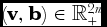 $(\mathbf {v},\mathbf {b}) \in \mathbb {R}^{2n}_+$, and any
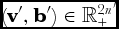 $(\mathbf {v}^{\prime },\mathbf {b}^{\prime }) \in \mathbb {R}^{2n^{\prime }}_+$, the statement (v, b)R(v′, b′) is interpreted as saying that the viability–fecundity pair (v, b) exhibits at least as much group fitness as the viability–fecundity pair (v′, b′). If I (resp. P) is substituted for R, then ‘the same’ (resp. ‘strictly more’) replaces ‘at least as much’ in the preceding statement.
By defining R on Ω, it is implicitly assumed that there are no a priori upper bounds on a cell's viability or fecundity. The validity of this assumption depends on how viability and fecundity are measured. If, for example, a cell's viability is the probability that it will survive long enough to reproduce, then it is not possible for viability to exceed one. The characterization theorem presented here also holds if there are upper bounds on the individual viabilities and fecundities but, for simplicity, such bounds are ignored. In some applications (see below), individual viabilities or fecundities may only take on integer values. In such cases, the assumption that non-integer values are possible is a convenient approximation. Michod et al. (Reference Michod, Viossat, Solari, Hurand and Nedelcu2006) allow the individual viabilities and fecundities to have arbitrary nonnegative values, which permits them to use the methods of differential calculus to identify a solution to the fitness maximization problem.
Excluding the possibility that a group is composed of cells none of which is viable or none of which is fecund allows for a simpler statement of the characterization theorem than would be possible without this assumption. An organism with no viable cells or no fecund cells is of no biological interest, so this restriction is quite natural. If there is complete germ-soma specialization, a cell has zero viability if and only if it has positive fecundity.
Michod et al. (Reference Michod, Viossat, Solari, Hurand and Nedelcu2006) make group fitness comparisons using a group fitness index that assigns a fitness value to each viability–fecundity profile. Their index is constructed in two steps by first computing measures of group viability and fecundity and then taking the product of these two values. Formally, for a group of size n, group viability is
 \begin{equation}
v = \sum _{i=1}^n v_i
\end{equation}
 \begin{equation}
b = \sum _{i=1}^n b_i.
\end{equation}
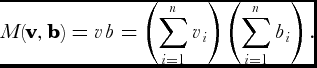
 $M: \Omega \rightarrow \mathbb {R}$ that measures fitness by taking the product of group viability and group fecundity.Footnote 7 That is, for all
 $n \in \mathbb {N}$ and all (v, b) ∈ Ωn, the value of the MVSHN index is
 \begin{equation}
M(\mathbf {v},\mathbf {b}) = v b = \left(\sum _{i=1}^n v_i \right) \left( \sum _{i=1}^n b_i \right).
\end{equation}
The MVSHN index in (3) can capture the fitness advantages of germ-soma specialization. Such specialization contributes to both group viability v and group fecundity b and, hence, to group fitness. This is not the case if group fitness is measured by the sum or average of the individual cell fitnesses. The fitness of cell i is
 \begin{equation}
f_i = v_i b_i.
\end{equation}
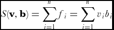
 $S: \Omega \rightarrow \mathbb {R}$ defined by taking the sum of the individual fitnesses in (4), whereas the average group fitness index the function
 $A: \Omega \rightarrow \mathbb {R}$ defined by taking their average. Formally, S and A are defined by setting, for all
 $n \in \mathbb {N}$ and all (v, b) ∈ Ωn,
 \begin{equation}
S(\mathbf {v},\mathbf {b}) = \sum _{i=1}^n f_i = \sum _{i=1}^n v_i b_i
\end{equation}
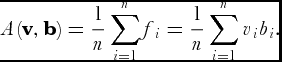 \begin{equation}
A(\mathbf {v},\mathbf {b}) = \frac{1}{n} \sum _{i=1}^n f_i = \frac{1}{n} \sum _{i=1}^n v_i b_i.
\end{equation}
The MVSHN group fitness ordering RM of Ω is defined by letting
 \begin{equation}
(\mathbf {v},\mathbf {b}) R^M (\mathbf {v}^{\prime },\mathbf {b}^{\prime }) \; \Leftrightarrow \; M(\mathbf {v},\mathbf {b}) \ge M(\mathbf {v}^{\prime },\mathbf {b}^{\prime })
\end{equation}
 $n,n^{\prime } \in \mathbb {N}$, all (v, b) ∈ Ω2n, and all (v′, b′) ∈ Ω2n′. That is, the viability–fecundity profile (v, b) exhibits at least as much group fitness as (v′, b′) if and only if the former has at least as large a value of the MVSHN index as the latter. In order to determine the characteristics of a group that maximizes fitness given the constraints that it faces, only the ordering induced by the group fitness index is relevant, not the numerical values assigned by the index to each viability–fecundity profile. For this reason, the MVSHN group fitness ordering RM rather than the MVSHN group fitness index M is axiomatized here.
3. PROPERTIES OF GROUP FITNESS ORDERINGS
In the next section, we axiomatically characterize the MVSHN group fitness ordering. In this section, we provide formal statements and biological interpretations of the axioms used in this characterization.
The axioms can be divided into three categories. Those in the first two categories concern group fitness comparisons involving the same number of cells. These axioms can be categorized according to their scope in the following sense. There are two components to fitness – viability and fecundity. If an axiom applies to comparisons in which both of these components may differ, then it is an intercomponent axiom. If, on the other hand, only one of the components differs, then it is an intracomponent axiom. The third category consists of a single variable group size axiom that is concerned with comparisons across group sizes.
The first three properties for a group fitness ordering are intercomponent axioms.
Intercomponent Separability. For all  $n \in \mathbb {N}$ and all (v, b), (v′, b′) ∈ Ω2n,
 \begin{eqnarray*}
[((\mathbf {v},\mathbf {b}) R (\mathbf {v}^{\prime },\mathbf {b}) \; \Leftrightarrow \; (\mathbf {v},\mathbf {b}^{\prime }) R (\mathbf {v}^{\prime },\mathbf {b}^{\prime })] \; \; \mbox{ and } \; \; [(\mathbf {v},\mathbf {b}) R (\mathbf {v},\mathbf {b}^{\prime }) \; \Leftrightarrow \; (\mathbf {v}^{\prime },\mathbf {b}) R (\mathbf {v}^{\prime },\mathbf {b}^{\prime })].
\end{eqnarray*}
 \begin{equation}
\mathbf {v} R_n^v \mathbf {v}^{\prime } \; \Leftrightarrow \; (\mathbf {v},\mathbf {b}^0) R (\mathbf {v}^{\prime },\mathbf {b}^0)
\end{equation}
 \begin{equation}
\mathbf {b} R_n^b \mathbf {b}^{\prime } \; \Leftrightarrow \; (\mathbf {v}^0,\mathbf {b}) R (\mathbf {v}^0,\mathbf {b}^{\prime })
\end{equation}
Intercomponent Ratio-Scale Measurability. For all  $n \in \mathbb {N}$, all (v, b), (v′, b′) ∈ Ω2n, and all γv, γb > 0,
 \begin{eqnarray*}
(\mathbf {v},\mathbf {b}) R (\mathbf {v}^{\prime },\mathbf {b}^{\prime }) \; \Leftrightarrow \; (\gamma ^v \mathbf {v}, \gamma ^b \mathbf {b}) R (\gamma ^v \mathbf {v}^{\prime }, \gamma ^b \mathbf {b}^{\prime }).
\end{eqnarray*}
Intercomponent Symmetry. For all  $n \in \mathbb {N}$ and all (v, b) ∈ Ω2n,
 \begin{eqnarray*}
(\mathbf {v},\mathbf {b}) I (\mathbf {b},\mathbf {v}).
\end{eqnarray*}
Next, two intracomponent axioms are considered.
Intracomponent Minimal Increasingness. For all  $n \in \mathbb {N}$, all (v, b), (v′, b′) ∈ Ω2n, and all α, β > 0 such that α > β,
 \begin{eqnarray*}
(\alpha \mathbf {1}^n,\mathbf {b}) P (\beta \mathbf {1}^n,\mathbf {b}) \; \; \mbox{ and } \; \; (\mathbf {v},\alpha \mathbf {1}^n) P (\mathbf {v},\beta \mathbf {1}^n).
\end{eqnarray*}
Intracomponent Incremental Symmetry. For all  $n \in \mathbb {N}$, all (v, b) ∈ Ω2n, and all i, j ∈ Nn,
(i) for all
 $\delta \in \mathbb {R}$ such that (v + δ1ni), (v + δ1nj) ∈ Ωn,
\begin{eqnarray*}
(\mathbf {v} + \delta \mathbf {1}^n_i,\mathbf {b}) I (\mathbf {v} + \delta \mathbf {1}^n_j,\mathbf {b});
\end{eqnarray*}
(ii) for all
$\delta \in \mathbb {R}$ such that (b + δ1ni), (b + δ1nj) ∈ Ωn,
\begin{eqnarray*}
(\mathbf {v}, \mathbf {b} + \delta \mathbf {1}^n_i) I (\mathbf {v}, \mathbf {b} + \delta \mathbf {1}^n_j).
\end{eqnarray*}




This axiom captures a way in which the contributions of the cells to group fitness are symmetric. Specifically, it requires that the change in group fitness as a result of either an increase or a decrease in a cell's viability or fecundity to be independent of which cell undergoes this change. In its social choice formulation, this axiom says that it is a matter of social indifference which individual experiences a given change in utility (Blackorby et al. Reference Blackorby and Donaldson2002).
The final property is the only variable group size axiom.
Null Cell Invariance. For all  $n \in \mathbb {N}$ and all (v, b) ∈ Ω2n,
 \begin{eqnarray*}
(\mathbf {v}, \mathbf {b}) I ( (\mathbf {v},0),(\mathbf {b},0) ).
\end{eqnarray*}
4. AN AXIOMATIC CHARACTERIZATION OF THE MVSHN GROUP FITNESS ORDERING
Our main result shows that the MVSHN group fitness ordering is characterized by the six axioms introduced in the preceding section. The proof of this theorem proceeds by first showing that these axioms imply that the MVSHN group fitness ordering must be used to compare viability–fecundity profiles for groups with the same number of cells. This is done in a series of four lemmas. The proofs of these lemmas make use of proof strategies employed by Blackorby et al. (Reference Blackorby and Donaldson2002) and Ooghe and Lauwers (Reference Ooghe and Lauwers2005). The proof of the theorem is completed by showing that the MVSHN group fitness ordering must also be used when the number of cells in the groups being compared differ.
Lemma 1 demonstrates that Intercomponent Separability by itself implies that group fitness comparisons can be decomposed into comparisons of group viability and group fecundity.
Lemma 1.If the group fitness ordering R satisfies Intercomponent Separability, then for all  $n \in \mathbb {N}$, there exist orderings Rvn and Rbn of Ωnsuch that for all (v, b), (v′, b′) ∈ Ω2n,
(i) [vRvn v′ and bRvn b′] ⇒ (v, b)R(v′, b′);
(ii) [vPvn v′ and bRbn b′] ⇒ (v, b)P(v′, b′);
(iii) [vRvn v′ and bPbn b′] ⇒ (v, b)P(v′, b′).
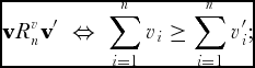
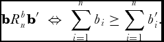
The ordering Rvn provides an ordering of viability profiles in terms of group viability. Similarly, the ordering Rbn provides an ordering of fecundity profiles in terms of group fecundity. These orderings are the conditional orderings defined in (8) and (9). Furthermore, if one group exhibits at least as much group viability and group fecundity as a second, then the first group is at least as fit overall as the second. If, in addition, either the group viability or group fecundity ordering is strict, then so is the group fitness ordering.
With the addition of Intracomponent Minimal Increasingness and Intracomponent Incremental Symmetry to Intercomponent Separability, Lemma 2 shows that the group viability ordering Rvn and the group fecundity ordering Rbn can be represented by indices of group viability and group fecundity that take the additive forms in (1) and (2). That is, group viability (resp. fecundity) is the sum of the individual cell viabilities (resp. fecundities).
Lemma 2.If the group fitness ordering R satisfies Intercomponent Separability, Intracomponent Minimal Increasingness, and Intracomponent Incremental Symmetry, then the orderings Rvn and Rbn established in Lemma 1 are such that
(i) for all v, v′ ∈ Ωn,
\begin{eqnarray*}
\mathbf {v} R_n^v \mathbf {v}^{\prime } \; \Leftrightarrow \; \sum _{i=1}^n v_i \ge \sum _{i=1}^n v^{\prime }_i;
\end{eqnarray*}
(ii) for all b, b′ ∈ Ωn,
\begin{eqnarray*}
\mathbf {b} R_n^b \mathbf {b}^{\prime } \; \Leftrightarrow \; \sum _{i=1}^n b_i \ge \sum _{i=1}^n b^{\prime }_i.
\end{eqnarray*}
It has now been established that for comparisons for a fixed number of cells, group fitness is a function of indices of group viability and group fecundity that have the additive functional form used in the MVSHN index. It remains to show that group fitness is obtained by multiplying the values of these group viability and group fecundity indices. A necessary condition for this to be the case is that group fitness is unchanged if all of the cell viabilities are multiplied by a positive constant γ and all of the cell fecundities are multiplied by its reciprocal 1/γ. The corresponding property for a social welfare ordering is called the multiplicative principle (Ooghe and Lauwers Reference Ooghe and Lauwers2005). Lemma 3 shows that the group fitness ordering R satisfies the multiplicative principle if it satisfies Intercomponent Ratio-Scale Measurability and Intercomponent Symmetry.
Lemma 3.If the group fitness ordering R satisfies Intercomponent Ratio-Scale Measurability and Intercomponent Symmetry, then for all  $n \in \mathbb {N}$, all (v, b) ∈ Ω2n, and all γ > 0,
 \begin{eqnarray*}
(\mathbf {v},\mathbf {b}) I (\gamma \mathbf {v}, (1/\gamma ) \mathbf {b}).
\end{eqnarray*}
Lemma 4.If the group fitness ordering R satisfies Intercomponent Separability, Intercomponent Ratio-Scale Measurability, Intercomponent Symmetry, Intracomponent Minimal Increasingness, and Intracomponent Incremental Symmetry, then for all  $n \in \mathbb {N}$, the restriction of R to Ω2nis equal to the restriction of the MVSHN group fitness ordering RM to Ω2n.
Theorem 1 provides an axiomatic characterization of the MVSHN group fitness ordering. It shows that the six axioms considered here are necessary and sufficient for the group fitness ordering R to be the MVSHN group fitness ordering RM. The addition of the Null Cell Invariance axiom to the other five axioms implies that RM must be used to make group fitness comparisons when the number of cells differ, not only when they are the same. A comparison of viability–fecundity profiles for two groups with different numbers of cells can be transformed into a comparison for the same number of cells by adding null cells to the smaller group until the number of cells in the two groups are equalized. A null cell has no viability or fecundity, so the addition of such a cell has no effect on the fitness of the initially smaller group. It is because the addition of a null cell has no effect on group viability or group fecundity as measured in the MVSHN index and, hence, on their product, that the MVSHN index must be used for all group fitness comparisons, not just for comparing groups with the same number of cells. It is straightforward to verify that all six axioms are satisfied by RM.
Theorem 1.The group fitness ordering R satisfies Intercomponent Separability, Intercomponent Ratio-Scale Measurability, Intercomponent Symmetry, Intracomponent Minimal Increasingness, Intracomponent Incremental Symmetry, and Null Cell Invariance if and only if R is the MVSHN group fitness ordering RM.
The six axioms in Theorem 1 are independent. Hence, any five of them are satisfied by other group fitness orderings in addition to RM. The ordering RM also satisfies other properties that are not independent of those in the theorem statement. Two of them are described below.
Strict Monotonicity. For all  $n \in \mathbb {N}$ and all (v, b), (v′, b′) ∈ Ω2n,
 \begin{eqnarray*}
(\mathbf {v},\mathbf {b}) > (\mathbf {v}^{\prime },\mathbf {b}^{\prime }) \; \Rightarrow \; (\mathbf {v},\mathbf {b}) P (\mathbf {v}^{\prime },\mathbf {b}^{\prime }).
\end{eqnarray*}
Continuity. For all  $n \in \mathbb {N}$ and all (v, b) ∈ Ω2n, the sets {(v′, b′) ∈ Ω2n∣(v′, b′)R(v, b)} and {(v′, b′) ∈ Ω2n∣(v, b)R(v′, b′)} are both closed. Informally, Continuity requires a small change in the viability–fecundity profile to have only a small effect on group fitness. The ordering RM satisfies this property because the MVSHN group fitness index M is continuous in its arguments.
5. CONCLUDING REMARKS
The MVSHN group fitness index M and its associated group fitness ordering RM were designed to show that, at least in some circumstances, germ-soma specialization is a property of the solution to a formal constrained group fitness optimization problem in which M is the objective function. But, as Michod et al. (Reference Michod, Viossat, Solari, Hurand and Nedelcu2006) note, this conclusion can also be obtained using other group fitness indices. Which is the most appropriate index to use to analyse a unicellular–multicellular transition depends on the multicellular lineage being considered. Knowing the properties that characterize different candidate group fitness orderings can help identify which one of them best describes how the evolution of group fitness is related to the characteristics of a lineage.
In spite of their advantages, M and RM are not suitable for analysing group fitness during all stages of a unicellular–multicellular transition. The problem is that the functional form of M is independent of group size. However, during the early stages of a transition, the group is not well integrated, so the evolutionary forces that it is being subjected to are best described by multilevel selection 1. But, in that case, the sum or average of the individual fitnesses, not the MVSHN index, measures group fitness. It is only in the later stages of the transition that it is more appropriate to measure group fitness with an index like the MVSHN index that separately accounts for the contributions to group fitness of the viabilities and fecundities of the individual cells.
This observation suggests that some of the axioms that characterize the MVSHN group fitness ordering should not be applied for all group sizes. If viability–fecundity profiles are compared using the sum group fitness index S, then all the axioms are satisfied except for Intercomponent Separability and Intracomponent Incremental Symmetry. When there is little or no germ-soma specialization, the contribution that a cell's viability (resp. fecundity) makes to group fitness depends more on this cell's fecundity (resp. viability) than either of these axioms permit. When the average group fitness index A is used instead of S to make group fitness comparisons, Null Cell Invariance is violated in addition to Intercomponent Separability and Intracomponent Incremental Symmetry. A cell with no viability or fecundity has no fitness, so the addition of such a cell reduces average cell fitness.
Here, the axiomatic method has been employed to factor the MVSHN group fitness index into its constitutive properties. This methodology can also be used to help construct a different group fitness index that is better suited for analysing any particular evolutionary transition. This is done by first identifying the properties that the index should satisfy if it is to accurately describe the fitness of the lineage being considered and then determining which group fitness indices satisfy these properties.
The MVSHN index only depends on the individual cell viabilities and fecundities. Other cell properties might also be important determinants of group fitness, such as the ease with which cells adhere to or communicate with other cells (Rokas Reference Rokas2008). If so, then a group fitness ordering should also depend on these properties. The social choice approach employed here to study group fitness can easily take factors such as these into account.
APPENDIX
Proof of Lemma 1. Suppose that R satisfies Intercomponent Separability. Consider any  $n \in \mathbb {N}$ and any (v0, b0) ∈ Ω2n. Let Rvn and Rbn be the binary relations on Ωn defined in (8) and (9), respectively. By Intercomponent Separability, Rvn and Rbn are independent of the choice of v0 and b0. Because R is an ordering, Rvn and Rbn are orderings as well.
(i) Suppose that vRvn v′ and bRbn b′. By the definitions of Rvn and Rbn,
 \begin{eqnarray*}
(\mathbf {v},\mathbf {b}^0) R (\mathbf {v}^{\prime },\mathbf {b}^0) \; \mbox{ and } \; (\mathbf {v}^0,\mathbf {b}) R (\mathbf {v}^0,\mathbf {b}^{\prime }).
\end{eqnarray*}
 \begin{eqnarray*}
(\mathbf {v},\mathbf {b}) R (\mathbf {v}^{\prime },\mathbf {b}) \; \mbox{ and } \; (\mathbf {v}^{\prime },\mathbf {b}) R (\mathbf {v}^{\prime },\mathbf {b}^{\prime }).
\end{eqnarray*}
(ii) Suppose that vPvn v′ and bRbn b′. By the definitions of Rvn and Rbn,
 \begin{eqnarray*}
(\mathbf {v},\mathbf {b}^0) P (\mathbf {v}^{\prime },\mathbf {b}^0) \; \mbox{ and } \; (\mathbf {v}^0,\mathbf {b}) R (\mathbf {v}^0,\mathbf {b}^{\prime }).
\end{eqnarray*}
 \begin{eqnarray*}
(\mathbf {v},\mathbf {b}) P (\mathbf {v}^{\prime },\mathbf {b}) \; \mbox{ and } \; (\mathbf {v}^{\prime },\mathbf {b}) R (\mathbf {v}^{\prime },\mathbf {b}^{\prime }).
\end{eqnarray*}
(iii) The proof of (iii) parallels that of (ii) with the roles of viability and fecundity interchanged. □
Proof of Lemma 2. Lemma 1 ensures that the orderings Rvn and Rbn exist.
(i) Consider any v ∈ Ωn. If v 1 = ⋅⋅⋅ = vn, it follows immediately that
 \begin{eqnarray*}
v_j = \frac{1}{n} \sum _{i=1}^n v_i
\end{eqnarray*}
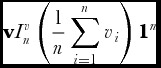 \begin{equation}
\mathbf {v} I_n^v \left( \frac{1}{n} \sum _{i=1}^n v_i \right) \mathbf {1}^n
\end{equation}
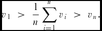 \begin{equation}
v_1 \; > \; \frac{1}{n} \sum _{i=1}^n v_i \; > \; v_n.
\end{equation}
 \begin{equation}
\mathbf {v} I_n^v (\mathbf {v} - \delta \mathbf {1}^n_1 + \delta \mathbf {1}^n_j).
\end{equation}
 \begin{eqnarray*}
\delta = \frac{1}{n} \sum _{i=1}^n v_i - v_j
\end{eqnarray*}
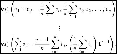 \begin{eqnarray*}
&\mathbf {v}I_n^v \left( v_1 + v_2 - \displaystyle\frac{1}{n} \sum\limits _{i=1}^n v_i, \displaystyle\frac{1}{n} \sum\limits _{i=1}^n v_i, v_3,\ldots ,v_n \right) \\
& \ \vdots \\
&\mathbf {v} I_n^v \left( \sum\limits _{i=1}^n v_i - \displaystyle\frac{n-1}{n} \sum\limits _{i=1}^n v_i, \left( \displaystyle\frac{1}{n} \sum\limits _{i=1}^n v_i \right) {\bf 1}^{n-1} \right).
\end{eqnarray*}
 \begin{eqnarray*}
\left( \sum _{i=1}^n v_i - \frac{n-1}{n} \sum _{i=1}^n v_i, \left( \frac{1}{n} \sum _{i=1}^n v_i \right) {\bf 1}^{n-1} \right) = \left( \frac{1}{n} \sum _{i=1}^n v_i \right) {\bf 1}^n,
\end{eqnarray*}
Now consider any v, v′ ∈ Ωn. By applying (A.1) to v and to v′, it follows that
 \begin{eqnarray*}
\mathbf {v} I_n^v \left( \frac{1}{n} \sum _{i=1}^n v_i \right) {\bf 1}^n \; \; \mbox{ and } \; \; \mathbf {v}^{\prime } I_n^v \left( \frac{1}{n} \sum _{i=1}^n v^{\prime }_i \right) {\bf 1}^n.
\end{eqnarray*}
 \begin{eqnarray*}
\mathbf {v} R^v_n \mathbf {v}^{\prime } \; \Leftrightarrow \; \left( \frac{1}{n} \sum _{i=1}^n v_i \right) {\bf 1}^n R^v_n \left( \frac{1}{n} \sum _{i=1}^n v^{\prime }_i \right) {\bf 1}^n.
\end{eqnarray*}
 \begin{eqnarray*}
\mathbf {v} R^v_n \mathbf {v}^{\prime } \; \Leftrightarrow \; \frac{1}{n} \sum _{i=1}^n v_i \ge \frac{1}{n} \sum _{i=1}^n v^{\prime }_i \; \Leftrightarrow \; \sum _{i=1}^n v_i \ge \sum _{i=1}^n v^{\prime }_i ,
\end{eqnarray*}
(ii) The proof of the second part of the lemma is analogous to that of the first with viability replaced by fecundity. □
Proof of Lemma 3. Consider any  $n \in \mathbb {N}$, any (v, b), (v′, b′) ∈ Ω2n, and any γ > 0. By Intercomponent Ratio-Scale Measurability,
 \begin{equation}
(\mathbf {v},\mathbf {b}) R (\mathbf {v}^{\prime },\mathbf {b}^{\prime }) \; \Leftrightarrow \; (\gamma \mathbf {v},\mathbf {b}) R (\gamma \mathbf {v}^{\prime },\mathbf {b}^{\prime }).
\end{equation}
 \begin{equation}
(\gamma \mathbf {v}^{\prime },\mathbf {b}^{\prime }) I (\mathbf {b}^{\prime }, \gamma \mathbf {v}^{\prime }).
\end{equation}
 \begin{equation}
(\mathbf {v},\mathbf {b}) R (\mathbf {v}^{\prime },\mathbf {b}^{\prime }) \; \Leftrightarrow \; (\gamma \mathbf {\mathbf {v}},\mathbf {b}) R (\mathbf {b}^{\prime },\gamma \mathbf {v}^{\prime }).
\end{equation}
 \begin{equation}
(\gamma \mathbf {v},\mathbf {b}) R (\mathbf {b}^{\prime },\gamma \mathbf {v}^{\prime }) \; \Leftrightarrow \; (\gamma \mathbf {v},(1/\gamma ) \mathbf {b}) R (\mathbf {b}^{\prime },\mathbf {v}^{\prime })
\end{equation}
 \begin{equation}
(\mathbf {b}^{\prime },\mathbf {v}^{\prime }) I (\mathbf {v}^{\prime },\mathbf {b}^{\prime }).
\end{equation}
 \begin{equation}
(\gamma \mathbf {v},\mathbf {b}) R (\mathbf {b}^{\prime },\gamma \mathbf {v}^{\prime }) \; \Leftrightarrow \; (\gamma \mathbf {v},(1/\gamma )\mathbf {b}) R (\mathbf {v}^{\prime },\mathbf {b}^{\prime }).
\end{equation}
 \begin{equation}
(\mathbf {v},\mathbf {b}) R (\mathbf {v}^{\prime },\mathbf {b}^{\prime }) \; \Leftrightarrow \; (\gamma \mathbf {v},(1/\gamma )\mathbf {b}) R (\mathbf {v}^{\prime },\mathbf {b}^{\prime }).
\end{equation}
 \begin{eqnarray*}
(\mathbf {v},\mathbf {b}) R (\mathbf {v},\mathbf {b}) \; \Leftrightarrow \; (\gamma \mathbf {v},(1/\gamma )\mathbf {b}) R (\mathbf {v},\mathbf {b}),
\end{eqnarray*}
 \begin{eqnarray*}
(\mathbf {v},\mathbf {b}) I (\gamma \mathbf {v},(1/\gamma )\mathbf {b}),
\end{eqnarray*}
Proof of Lemma 4. Consider any  $n \in \mathbb {N}$ and any (v, b), (v′, b′) ∈ Ω2n. It is sufficient to prove that
(i) (v, b)IM(v′, b′) ⇒ (v, b)I(v′, b′)
and
(ii) (v, b)PM(v′, b′) ⇒ (v, b)P(v′, b′).
(i) Suppose that (v, b)IM(v′, b′). That is, by (3) and (7),
 \begin{equation}
\left( \sum _{i=1}^n v_i \right) \left( \sum _{i=1}^n b_i \right) = \left( \sum _{i=1}^n v^{\prime }_i \right) \left( \sum _{i=1}^n b^{\prime }_i \right).
\end{equation}
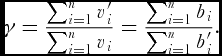 \begin{equation}
\gamma = \displaystyle\frac{\sum _{i=1}^n v^{\prime }_i}{\sum _{i=1}^n v_i} = \displaystyle\frac{\sum _{i=1}^n b_i}{\sum _{i=1}^n b^{\prime }_i}.
\end{equation}
 $\Omega ^n = \mathbb {R}^n_+ \setminus \lbrace \mathbf {0}^n \rbrace$ and, thus, the sums in the above denominators are non-zero. Rearranging these equalities, it follows that
 \begin{equation}
\sum _{i=1}^n v^{\prime }_i = \sum _{i=1}^n \gamma v_i \; \; \mbox{ and } \; \; \sum _{i=1}^n b^{\prime }_i = \sum _{i=1}^n \frac{1}{\gamma } b_i.
\end{equation}
 \begin{equation}
\gamma \mathbf {v} I_n^v \mathbf {v}^{\prime } \; \; \mbox{ and } \; \; (1/\gamma ) \mathbf {b} I_n^b \mathbf {b}^{\prime }.
\end{equation}
 \begin{equation}
(\gamma \mathbf {v}, (1/\gamma )\mathbf {b}) I (\mathbf {v}^{\prime },\mathbf {b}^{\prime }).
\end{equation}
 \begin{equation}
(\mathbf {v},\mathbf {b}) I (\gamma \mathbf {v}, (1/\gamma )\mathbf {b}).
\end{equation}
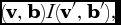 \begin{equation}
(\mathbf {v},\mathbf {b}) I (\mathbf {v}^{\prime },\mathbf {b}^{\prime }) ,
\end{equation}
(ii) Now, suppose that (v, b)PM(v′, b′). The proof is the same as the proof of case (i) with the following modifications. The equality in (A.11) is replaced by > and the second equalities in (A.12) and (A.13) are replaced by <. In (A.14), Ibn is replaced by Pbn and in (A.15) and (A.17), I is replaced by P. □
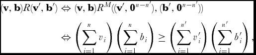
Proof of Theorem 1. That RM satisfies the requisite axioms is straightforward to verify. Lemma 4 has established that, given the axioms in the theorem statement, comparisons involving the same number of cells must be carried out with the ordering RM. Thus, the proof is complete once it is established that the same is true for comparisons involving different numbers of cells.
Consider any  $n,n^{\prime } \in \mathbb {N}$ with n≠n′, any (v, b) ∈ Ω2n, and any (v′, b′) ∈ Ω2n′. Without loss of generality, suppose that n > n′. By (repeated if necessary) application of Null Cell Invariance (and transitivity), it follows that
 \begin{eqnarray*}
(\mathbf {v}^{\prime },\mathbf {b}^{\prime }) I ( (\mathbf {v}^{\prime },\mathbf {0}^{n-n^{\prime }}),(\mathbf {b}^{\prime },\mathbf {0}^{n-n^{\prime }} ) ).
\end{eqnarray*}
 \begin{equation}
(\mathbf {v},\mathbf {b}) R (\mathbf {v}^{\prime },\mathbf {b}^{\prime }) \; \Leftrightarrow \; (\mathbf {v},\mathbf {b}) R ( (\mathbf {v}^{\prime },\mathbf {0}^{n-n^{\prime }}),(\mathbf {b}^{\prime },\mathbf {0}^{n-n^{\prime }}) ).
\end{equation}
 \begin{eqnarray*}
(\mathbf {v},\mathbf {b}) R (\mathbf {v}^{\prime },\mathbf {b}^{\prime }) & \Leftrightarrow& (\mathbf {v},\mathbf {b}) R^M ( (\mathbf {v}^{\prime },\mathbf {0}^{n-n^{\prime }}),(\mathbf {b}^{\prime },\mathbf {0}^{n-n^{\prime }}) ) \\
& \Leftrightarrow& \left( \sum _{i=1}^n v_i \right) \left( \sum _{i=1}^n b_i \right) \ge \left( \sum _{i=1}^{n^{\prime }} v^{\prime }_i \right) \left( \sum _{i=1}^{n^{\prime }} b^{\prime }_i \right),
\end{eqnarray*}


