

1 Introduction
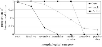
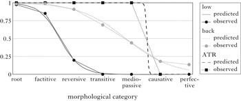
In Tommo So, a Dogon language of Mali, there are three vowel-harmony processes, all optional. Our focus is on the fact that, for all three processes, frequency of application interacts with morphological structure: intuitively, harmony ‘peters out’, in the sense that it applies with gradually diminishing frequency in outer layers of the morphology (defined by the possibilities of affix order, following Kiparsky Reference Kiparsky1982). Each process peters out at a different rate: Low Harmony first (applying only within the innermost morphological layers), Backness Harmony next and ATR Harmony last. The graph in Fig. 1 gives the basic pattern.
Tommo So vowel harmony: application rates by morphological layer.

We propose a formal model of this pattern, drawing on two ideas in phonological theory: Harmonic Grammar and scalar constraints. We show that this model achieves a far better fit to the data than a number of alternatives, notably the inverted exponential model of Guy (Reference Guy1991).
Our paper is structured as follows: in §2 we review a crucial generalisation from Kiparsky that establishes the theoretical context of our work. §3 gives basic background (the vowel inventory and verbal morphology of Tommo So), then motivates the morphological layers with data from affix ordering. In §4, we illustrate the three vowel-harmony processes, and give the quantitative data. §5 applies Guy's multiplicative model to our data and demonstrates that it provides a poor fit. §6 is the main analytic section: we propose a set of constraints and deploy them in Harmonic Grammar, achieving a greatly improved fit to the data. We show that our approach is restrictive: only certain frequency patterns can be generated. We also review other linguistic phenomena showing similar quantitative patterns. §7 addresses theories that can describe our data but are not restrictive. §8 covers residual issues, and §9 concludes.
2 The theoretical context: affix order and phonological process applicability
Our work pursues an insight from Kiparsky (Reference Kiparsky1982): affix ordering and the applicability of phonological processes tend to be closely correlated. Specifically, affixes that occur ‘closer to the root’, as diagnosed by ordering tests, characteristically trigger or undergo more phonological processes. Kiparsky suggests that this correlation is ‘a general property of languages’ (Reference Kiparsky1982: 11), and in light of this proposes a Strong Domain Hypothesis (Reference Kiparsky, Elert, Johansson and Strangert1984: 142): ‘at lower levels of the lexicon and in the postlexical phonology rules may be ‘turned off’ but no new ones may be added’. Our Tommo So data follow this pattern, but in a gradient fashion (‘turning off’ is gradual); thus we will be treating the Kiparskian correlation in different theoretical terms.
We emphasise that the concept of root closeness on which Kiparsky relies is abstract: it is not the literal distance seen within individual forms, but is calculated by examining the morphology as a system. To give Kiparsky's example (Reference Kiparsky1982: 11): English has two negative prefixes, non- and in-, of which the latter may occur as il- by assimilation, as in illegible. When the two prefixes co-occur, non- may precede in-, but not vice versa: non-illegible but not *in-non-legible. This fact is reflected in the phonology: the process that assimilates /n/ to [l] before [l] is applicable to in- (illegal, illegible) but not to non- (*nol-legible). The essential correlation is between morphological distance – as reflected in the general affix-ordering principles – and phonological process application. It remains true that linearly, the non- of non-legible is just as close to the root (adjacent) as the il- of illegible; the criterion of distance is inferred from examination of the morphology as a whole.
We will see that Tommo So constitutes a far more elaborate case of the correlation of ‘closeness’, as diagnosed by affix order and phonology.
3 Background on Tommo So
3.1 Language and data sources
Tommo So is spoken by about 60,000 people living on the Bandiagara Escarpment in Mali (Hochstetler et al. Reference Hochstetler, Durieux and Durieux-Boon2004). It is documented in a reference grammar by McPherson (Reference McPherson2013). To our knowledge there has been no previous theoretical work on Tommo So vowel harmony; Hantgan & Davis (Reference Hantgan and Davis2012) treat harmony in the related Bondu-so, but the patterning of the latter system is quite different.
The data for this article were gathered by the first author in Mali during a total of 14 months of fieldwork between 2008 and 2012. There were four primary consultants, all from the commune of Tédié; their speech is relatively uniform, and it is reasonable to consider the data as reflecting one single dialect of Tommo So.
There exists no large corpus of Tommo So language material. The data we used were obtained by combing through the entirety of McPherson's field materials (consisting of an extensive lexicon, example sentences and a variety of narratives, traditional stories and conversations) for words containing any of the suffixes under consideration (§3.3); if the form contained no suffix vowel (due to vowel-hiatus resolution; see (11) below), it was deemed uninformative, and was not included. We mined this corpus (2818 forms) for the statistical generalisations given below. While the corpus is hardly a random sample, there is no reason to expect that the words obtained were biased concerning vowel harmony; most were elicited for other reasons, such as analysis of the morphology or of tone. Stylistically, the corpus is fairly uniform: 78% of forms come from elicited material. The full corpus is available in the supplementary materials.
3.2 The vowel system
The Tommo So vowel inventory is given in (1).
-
(1)


There are seven contrastive vowel qualities, [i e ε a ɔ o u]; minimal and near-minimal sets are given in (2a), with the corresponding long vowel phonemes illustrated in (2b). Long and short vowels of the same quality behave identically in harmony.Footnote 1
-
(2)
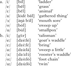
Additionally, [i] and [u] are often reduced to the high central vowel [ɨ] in medial position. In this environment, there is no phonemic contrast among the high vowels [i u ɨ]; what one hears is often phonetically intermediate. In faster speech [ɨ] normally appears, whereas in slower speech the output tends to be closer to [i] or [u]. The latter choice is determined in part by whether the reduced vowel is in a root or a suffix. In roots, the determining factor is normally the preceding vowel ([i e ε] tend to favour [i]-like qualities; [u o ɔ] favour [u]-like qualities). When the root vowel is [a], the quality of the reduced vowel is influenced by the place of articulation of neighbouring consonants (labials tend to prefer [u], coronals [i]). In the three suffixes that include a reduced vowel (reversive, transitive and mediopassive; §3.3), the reduced vowel tends to surface in slower speech as [i], though both [ɨ] and coarticulatorily induced [u] are also observed.
Vowel reduction is important phonologically, because reduced vowels are transparent to harmony. The underlying representations of reduced vowels is indeterminate (since their backness and rounding are not contrastive); we will, somewhat arbitrarily, give underlying representations with their most typical surface vowel.
We adopt the feature assignments for Tommo So vowels in (3); ∅ indicates underspecification. The feature [reduced] is employed as an ad hoc stand-in; in a fully formalised theory reduced vowels would be identified by their weak position in metrical structure.
-
(3)

The distribution of the feature [round] is predictable, since vowels are [+round] when [+back] and otherwise [−round]; for brevity we omit the straightforward rules or constraints that would be needed to fill in this value. It is sensible to treat [back] as the phonologically active feature; [a] turns out to be a non-trigger of Backness Harmony (see §4.3 below), and this may plausibly be related to the fact that it is phonetically neither front nor back. We leave [ATR] unspecified in non-mid vowels simply as an expression of agnosticism; we have no phonological or phonetic evidence to justify a classification.
3.3 Verbal morphology
In this section we give an overview of Tommo So verbal morphology, focusing on the suffixes that demonstrate the affiliation of affix ordering and harmony application; see McPherson (Reference McPherson2013: chs 11–12) for further detail. For simplicity at this preliminary stage we give examples that happen not to involve vowel harmony.
3.3.1 Derivational suffixes
The factitive, which we treat as underlying /-ndέ/, derives transitive verbs from intransitive ones (often with causative meaning), as in [dʑímέ] ‘be injured’ ~ [dʑímέ-ndέ] ‘injure’. It can also be used to derive inchoative verbs from adjectives (always in conjunction with the mediopassive suffix), as in [pàlá] ‘long’ ~ [pálá-nd-íjέ] ‘become long’.Footnote 2
The reversive suffix is /-ílέ/, as in [dὲbέ] ‘get stuck’ ~ [dὲb-ílέ] ‘get unstuck’, while transitive /-íɾέ/ denotes that the subject is performing the action of the verb to or on someone else, as in [tέmbέ] ‘find oneself in a situation’ ~ [tέmb-íɾέ] ‘make somebody find something’. Mediopassive /-íjέ/ denotes that the subject is performing the action on herself; thus [pέːndέ] ‘spread out (objects)’ ~ [pέːnd-íjέ] ‘(group) spread selves out’, and the causative suffix is /-mↄ́/, as in [sέmέ] ‘slaughter’ ~[sέmέ-mↄ́] ‘make slaughter’.
3.3.2 Inflectional suffixes
Only one inflectional suffix undergoes vowel harmony: the defocalised perfective, which is the version of the perfective employed when some element in the clause other than the verb is focused. This suffix has two allomorphs, /-ì/ and /-è/. Their distribution is somewhat complex, and the harmonic behaviour of the two is somewhat different. We will only discuss the /-ì/ allomorph in this paper, since the /-è/ allomorph never co-occurs with other suffixes, making it impossible to justify a morphological layer on the basis of affix ordering. For further discussion see McPherson (Reference McPherson2013: §12.4). An example of the /-ì/ allomorph is [nↄ́ːlↄ́] ‘mix’ ~ [nↄ̀ːl-ì] ‘mixed’.
There are a fair number of other inflectional suffixes, all of which appear outside of the derivational suffixes. None alternates by harmony. They include /-éːlè/ (negative imperfective), /-dὲ/ (affirmative imperfective), /-aː/ (perfective non-final), /-eː/ (imperfective non-final), /-lí/ (negative perfective), /-gú/ (negative imperative) and /-mↄ́/ (hortative).
3.4 The system of vowel phonemes in suffixes
We have seen above that a wide variety of contrasting vowel qualities appear in Tommo So verbal suffixes: /i u a e ε ɔ/ all occur (we assume the absence of /o/ is an accidental gap). This would likely defeat any effort to derive suffix vowel qualities by some sort of default insertion processes (as a reviewer suggested to us), and in what follows we will assume fully specified underlying suffix vowels.
3.5 Suffix ordering
Here we set out the principles of affix ordering in Tommo So, extending Kiparsky's ordering test to the more elaborate Tommo So ordering pattern. What emerges is a whole chain of pairwise orderings, diagnosing a system of morphological levels or layers.
To begin, we find that the factitive precedes the mediopassive, as in [pálá-nd-íjέ] (long-fact-mediopass) ‘become long’. The opposite order is never found (*[X-íjέ-ndέ]). The same test with other pairs yields the same result: only one order is possible. For brevity, we summarise the possible combinations in (4).
-
(4)
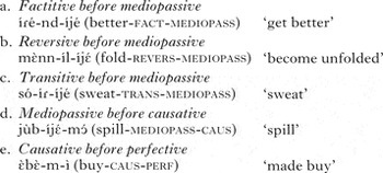
Moreover, the combinations we might expect on grounds of transitivity (like factitive before causative) are generally attested, a point we will not document here. Naturally, in some words there are multiple suffixes present, and these reflect the same ordering generalisations as the two-suffix forms; e.g. [àmà-nd-ìjὲ-m-ì] (rancid-fact-mediopass-caus-perf).
To test our affix-ordering principles, we used the entire database, extracting from it all words in which two or more verbal affixes attach to the same root. Ordering is entirely consistent: there are no cases whatsoever in which two affixes occur in the opposite order to that given in (4). However, there is one set of affixes (factitive, reversive, transitive) that never co-occur, and thus cannot be assessed for linear order. The results of our ordering study are given in (5) as a Hasse diagram.
-
(5)

For purposes of the analysis to follow, we elaborate these empirical findings into a system of morphological layers, as shown in (6), along the lines envisioned in the theory of Lexical Phonology (Kiparsky Reference Kiparsky1982, Reference Kiparsky1994, Reference Kiparsky2000, Reference Kiparsky, Féry and van de Vijver2003).
-
(6)
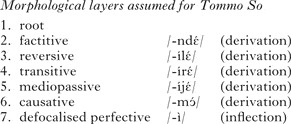
These reflect the ordering observations summarised in (5), but go further, in placing factitive, reversive and transitive in separate layers. The placement of transitive in a layer ‘outside’ factitive and reversive can be defended on the grounds that it is more productive and semantically transparent than the latter two suffixes; it is a characteristic of most level-ordered morphological systems that productive and transparent affixes gravitate to outer layers (see e.g. Katamba Reference Katamba2004). The same reasoning might also justify the placement of reversive outside factitive, although the difference in productivity is not as clear in this case.
The system of levels we propose relies on a set of assumptions about how children project the level system from learning data. Our suggestion is that children seek out the richest level system compatible with the data (in contradistinction to the ‘level-economising’ approach of classical Lexical Phonology), and that in setting up levels they rely on multiple sources of information. Of these, pairwise affix order is most crucial; that children attend closely to pairwise order is demonstrated by Ryan's (Reference Ryan2010) account of Tagalog. We also assume that children supplement ordering information with further evidence from transparency and productivity. The relatively elaborate structure of (6) is what emerges from this learning process. We suggest that a rich level system is not unique to Tommo So; parallel systems are seen wherever linguists have posited rich ‘position-class’ morphology, as in Athabaskan (e.g. Hargus Reference Hargus1988), Nimboran (Inkelas Reference Inkelas1993) and various of the languages given in Nida (Reference Nida1949).
4 The vowel-harmony pattern
With the principles of affix ordering in place, we turn to the other side of the Kiparskian correlation: the applicability of phonological processes, here vowel harmony.
We give the facts of Tommo So vowel harmony first in rule-based phonology (Chomsky & Halle Reference Chomsky and Halle1968), employed for its descriptive precision. In this framework, Tommo So would be considered to have three vowel-harmony rules, one each for the features [low], [back] and [ATR]. Since harmony is frequently optional, we will give examples for each harmony process of both application and non-application.
4.1 Verb roots
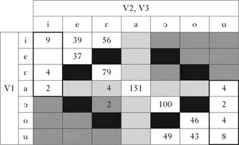
As in other languages (see e.g. Kiparsky Reference Kiparsky and Fujimura1973: 36 on Finnish and Clements & Sezer Reference Clements, Sezer, van der Hulst and Smith1982: 222–231 on Turkish), the vowel-harmony pattern applies slightly differently within roots and affixes, so we discuss the two separately. Harmony is also slightly different for verbs vs. nouns, and we will be focusing on verbs here. For roots, we give data based on a corpus of verbal roots (all of the affixes we discuss are verbal suffixes), which appears as Table I.
Sequences of vowels in Tommo So verb roots. Disharmonic sequences are shaded (ATR disharmonic=black; Backness disharmonic=dark grey; Low disharmonic=light grey).

The rows of Table I are labelled with the first vowel of a root, the columns with the second or third vowels (roots are maximally three syllables); thus the ‘9’ in the upper leftmost cell indicates nine cases in the corpus in which a root has [i] as its first vowel and [i] as its second or third vowel.
The boxed regions of the table, showing non-initial high vowels, require comment. In Tommo So, verb roots may not end in a high vowel; thus all of these high vowel counts represent medial high vowels in trisyllabic roots. As such, they are in the context for vowel reduction, and the observed distribution between [i] and [u] reflects the allophonic variation among reduced vowels noted in §3.2.
It is evident that many logically possible sequences of vowels are absent or severely underrepresented. These gaps are due to vowel harmony. The black cells represent forms excluded by ATR Harmony, the dark grey boxes represent forms excluded (with just two exceptions) by Backness Harmony, and the light grey boxes forms excluded (with just four exceptions) by Low Harmony. We turn now to a detailed description of each harmony process.
4.2 Low Harmony
We state Low Harmony as in (7).Footnote 3
-
(7)

Here X stands for any sequence, meaning that the rule can apply non-locally, affecting all the non-initial vowels of the word.Footnote 4 The surface pattern implied by (7) is as follows. [a] is never followed by a mid vowel ([−high, −low]), nor can it ever appear after an initial vowel other than [a]. Initial high vowels trigger Low Harmony, since in that position they are not reduced (§3.2). Thus, an initial high is never followed by [a]. But high vowels may follow initial [a], either because they are medial and therefore reduced, or because they occur in the defocalised perfective suffix and are therefore outside the domain of Low Harmony; see (12).
The effects of Low Harmony can be seen clearly in our verb-root corpus. Some representative data illustrating the patterns in Table I, as well as exceptions, are given in (8).
-
(8)
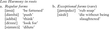
The words in (8b) represent two out of the total of only four exceptions in roots.
Consider next the behaviour of Low Harmony in suffixes. Because of ‘petering out’, Low Harmony affects only the two suffixes that form the innermost layers of the morphology in (6). The factitive suffix surfaces as [-ndá] when it follows a root with an initial low vowel, but as any of [-ndé], [-ndέ], [-ndó] or [-ndↄ́] in other contexts, depending on other vowel-harmony processes. /-ndέ/ is the underlying value, which surfaces when no harmony process applies.
-
(9)

The application rate of Low Harmony for factitive forms is about 85%. By this we mean that, of all cases in the data where a low-vowel root precedes the factitive suffix, 85% surface with a lowered factitive vowel. An example of non-application is [dʑàːndέ], which is the very same word as (9a), uttered by the same speaker on a different occasion.
We treat the reversive suffix as underlying /-ílέ/. For this suffix, the application rate of Low Harmony is only 20%. When Low Harmony applies, the reversive surfaces as [-ílá]; otherwise, it appears after [a] as its underlying form [-ílέ], or else as [-ílé], [-íló] or [-ílↄ́] where other vowel-harmony processes are applicable. It can be observed that application of Low Harmony to this suffix is non-local, skipping over the reduced suffix-initial vowel.
-
(10)

The forms in (10) illustrate another phonological process of Tommo So, the resolution of hiatus. Normally, when suffixation creates a sequence of two vowels, the first of the two is deleted (McPherson Reference McPherson2013: §3.7). The process is stated in (11).
-
(11)

Hiatus Resolution can be seen in (10), where the final /a/ deletes before suffix-initial /i/ (the second form in (10a) is an irregular case, with hiatus resolved by loss of the second vowel).
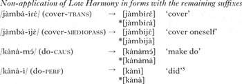
The remaining suffixes fall outside the domain in which Low Harmony applies. In (12), we give examples of its non-application for these suffixes.
-
(12)
Footnote 5
4.2.1 Excursus: defining application rate
Since application rates are the key data in this article, we take a moment to define them, using examples from the data just presented. There are four relevant categories, given in (13).
-
(13)

In what follows, we will define application rate by the formula in (14).
-
(14)

The numerator counts forms in which application produces an observable change, and the denominator counts all cases of potential applicability. This definition is used because it matches the criterion of adequacy for a constraint-based analysis (see §6 below). In cases of vacuous application or inapplicability, the faithful candidate incurs neither markedness nor faithfulness violations and will always win, making it uninformative about ranking or weighting.
4.3 Backness Harmony
The Backness Harmony pattern can be described with the rule in (15).
-
(15)

We first consider some details of the pattern. First, under the feature system we assume, [a] cannot be a trigger of Backness Harmony, since it has no backness value that can be transmitted to the target vowel. Hence [a] is compatible with both front and back following vowels. Moreover, it is impossible to tell if [a] is an undergoer of Backness Harmony, because there are no possible inputs; in roots, Low Harmony eliminates all non-initial [a]'s after backness-specified vowels, and there are no low-vowel suffixes in the layers of the morphology where harmony prevails. Second, Backness Harmony does not target reduced vowels (see §3.2 above), because, as noted above, their backness is gradient and determined by coarticulation.
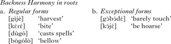
Turning to the data, we first illustrate Backness Harmony with data from roots, as summarised above in Table I. With very rare exceptions (about 1.7% of all forms), the front vowels [i e ε] may only co-occur with front vowels, and the back vowels [u o ɔ] only with back vowels (see the dark grey region of table). In (16) we give examples of both normal harmonic roots and the rare exceptions.
-
(16)
In suffixes, we find a consistent pattern of ‘petering out’ as we move morphologically away from the root. We consider the suffixes in order below.
In the factitive, Backness Harmony is virtually exceptionless; (17b) is the only exceptional form in the corpus. For completeness, we include cases of both vacuous and non-vacuous application.
-
(17)
Footnote 6 , Footnote 7

(17d) shows optional application of Low Harmony. It also forms part of the evidence that [a] is not a Backness Harmony trigger: in the variant where Low Harmony does not apply, we find [ε] as the suffix vowel, which reflects the underlying form. In all other forms in (17), the suffix also harmonises for the feature [ATR], to be discussed below.
The next morphological layer consists of the reversive suffix. Here Backness Harmony is only slightly less robust, applying to 91% of applicable forms.
-
(18)
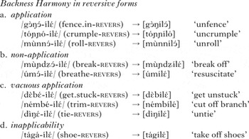
The vowel transcribed as [i] in these forms is a reduced vowel (see §3.2), and is hence skipped over by harmony. Once again, we see ATR alternations as well as backness alternations.
At the next morphological layer, transitive, the application rate of Backness Harmony drops to 69%. Again, we see that [a] is not a trigger, that the reduced vowel [i] in the suffix is transparent and that backness alternations are accompanied by ATR alternations.
-
(19)
Footnote 8 , Footnote 9 , Footnote 10

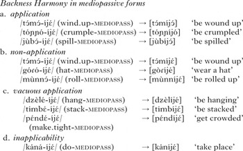
In the mediopassive (20), the application rate of Backness Harmony is 44%.
-
(20)
In the causative (21), the application rate is just 18%.
-
(21)

The form [kánámↄ́] in (21d) should be compared with (20d), [káníjέ]: the pair illustrates that [a] is not a Backness Harmony trigger and that the underlying backness value of the suffix surfaces after [a] roots; i.e. /-mↄ́/ vs. /-íjέ/. Since /-mↄ́/ is underlyingly [+back], our examples of non-application involve front-vowel roots.
Finally, in the defocalised perfective (22), the Backness Harmony rate is 14%.
-
(22)

All remaining morphology has a Backness Harmony rate of zero; by this point, Low and ATR Harmony have also petered out. Thus the suffixes (all inflectional; §3.3) have a single surface realisation.
4.4 ATR Harmony
The feature [ATR] is phonemic in Tommo So only for the class of mid vowels [e ε o ɔ]. It is these vowels that form both the trigger and target class for ATR Harmony, as stated in (23).
-
(23)

In verb roots, ATR Harmony is exceptionless: see Table I above, where the eight black boxes represent the eight logically possible sequences of disagreeing mid vowels ([e ε], [o ɔ], etc.). We give a few representative harmonic roots in (24).
-
(24)

The final form shows that even forms that are exceptions to Backness Harmony obey ATR Harmony.
The high vowels [i] and [u] are not ATR triggers (though see note 11 below): in roots they may co-occur with either the [+ATR] vowels [e o] or the [−ATR] vowels [ε ɔ], in either order, as shown in (25).
-
(25)

In principle, we could test our claim of non-triggerhood with suffix data, but due to the phonotactic restriction on high vowels in verb roots (§4.1), no actual cases arise: all roots contain at least one non-high vowel, and a high vowel will never be the closest vowel to the suffix. For this reason, the rule is formulated with the closest mid vowel as trigger rather than the initial vowel (as in Low Harmony and Backness Harmony).
The low vowel [a] likewise does not trigger ATR Harmony; after [a], suffixes surface unaltered for [ATR]. Thus the mid allomorph of the defocalised perfective (§3.3), which in general is harmonic, surfaces after [a] with its underlying value of [-è] (e.g. /bàlá-è/ (sweep-perf)→[bàlè] ‘swept’). All remaining mid-vowel suffixes have the underlying value [−ATR], and after [a], this is preserved; see below.
We now exemplify the applicability of ATR Harmony in each layer of the morphology. Here the data are far simpler, because the harmony rate is always either 100% or zero. For the factitive, reversive, transitive and mediopassive, the harmony rate is 100%. The actual allomorph that surfaces depends also on the other forms of harmony.Footnote 11
-
(26)

For the causative suffix, the harmony rate is zero. Hence it always surfaces as [−ATR]; usually [-mɔ] but sporadically [-mε], due to Backness Harmony.
4.5 Summary of suffix harmony
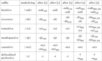
In Table II we summarise what has been said so far about suffix harmony.Footnote 12 The second column gives our proposed underlying representation for each suffix, and the remaining columns list the surface allomorphs as they appear after the five types of verb root (recall that due to verbal phonotactics there are no verb roots with all high vowels). All surface forms assumed to have undergone some harmony process non-vacuously are labelled. In each cell with more than one allomorph, the more frequent one is listed first.
Suffix allomorphs.

The factitive and reversive suffixes show a five-way alternation ([e~ε~a~ɔ~o]), since all three harmony processes apply to them. The transitive and mediopassive suffixes have only four allomorphs ([e~ε~ɔ~o]), since Low Harmony peters out before reaching them. The causative has just two allomorphs ([ε~ɔ]), determined by Backness Harmony, since ATR Harmony peters out before reaching it. The defocalised perfective likewise has only two allomorphs ([i~u]), determined by the only applicable harmony process, Backness Harmony.
4.6 Frequency of application
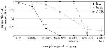
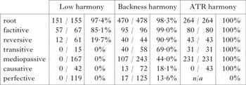
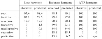
In Table III we compile the application rates reported above for all three harmony processes in all morphological contexts.Footnote 13 The frequency values represent token frequency, calculated by counting each instance of a repeated underlying form as a separate case. Moreover, where a form has two harmonising suffixes (none has three), it is counted twice, once for each suffix; this makes sense, because what we seek to model is the rate at which each suffix undergoes harmony. Application rates are also shown in Fig. 2, fleshing out Fig. 1; error bars represent 95% Clopper–Pearson binomial confidence intervals. As can be seen, for two of the harmony processes, application peters out gradually going outward from the root. ATR Harmony instead plummets from 100% to 0% at the mediopassive–causative break.
Tommo So vowel harmony: application rates by suffix and harmony type.

Application rates of vowel harmony by suffix and harmony process.

The two gradient processes peter out in a particular way, forming sigmoid (S-shaped) curves. When we turn to our analysis below (§6), our primary goal will be to derive this sigmoid shape in terms of principles which are well motivated in linguistic theory.
5 An earlier proposal: the inverted-exponential model
Before doing this, we first review what might be considered the ‘standard model’ for relating morphological distance to phonological process application, namely the widely cited proposal of Guy (Reference Guy1991). Guy developed his model in the course of studying simplification in English final C + {t,d} clusters, which likewise applies with lower frequency in outer layers of the morphology.
In Guy's model, the diminishing frequency of application emerges directly from the architecture of the grammar. He adopts the general approach to morphological layering assumed in the theory of Lexical Phonology and Morphology, in which layers are the result of a sequence of derivationally ordered levels. For English, the innermost level, Level 0, is the root; thus when the /t/ of a simplex form like act [ækt] is dropped in fluent speech, this is a case of a Level 0 /t/. The intermediate Level 1 is the domain of the /t/ that occurs as a non-productive past tense suffix, triggering stem allomorphy in words like kept [kεpt]. The outermost Level 2 is the domain of the regular past tense allomorph seen in words like tripped [tɹɪpt].
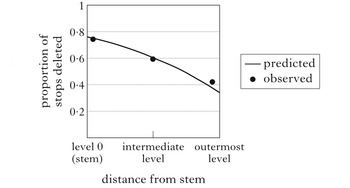
Studies examining the dropping of alveolar stops in consonant clusters have consistently found a petering out effect (Fasold Reference Fasold1972, Guy Reference Guy1980, Neu Reference Neu1980, Nesbitt Reference Nesbitt1984). For example, in Santa Ana's study of Chicano English (Reference Santa Ana1991), root-level alveolar stops are deleted 74.3% of the time, intermediate-level stops 59.3% and outermost-level stops 42.1%.
In Guy's model, such frequencies emerge from the system of level organisation. He proposes that the -t,d-deletion rule has a constant application rate, which can vary from dialect to dialect. Moreover, -t,d-deletion applies at all three morphological levels, and failure to apply on one level does not preclude application on a later level. Thus, for roots like act there are three chances for -t,d-deletion to apply, for kept there are two and for tripped there is just one, as shown in (27).
-
(27)

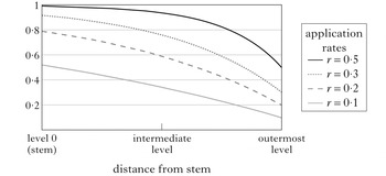
Assuming an application rate r, then after n chances to apply, the ‘survival rate’ is (1 − r) n and the application rate is therefore predicted to be 1−(1−r) n . If we plot application rate against n for various values of r, we get a family of inverted exponential curves, as in Fig. 3.
The inverted-exponential model: schematic predictions of application rate.

When a phonological process applies at more than one level, we can predict the application rate for all later levels using the inverted exponential formula (in the English case, given just one parameter, we predict three observed values). For the data from Santa Ana mentioned above, this is a fairly good fit, as shown in Fig. 4.Footnote 14
The inverted-exponential model applied to cluster simplication.

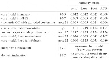
We applied the inverted-exponential model to the Tommo So data in Table III. Since we assume seven morphological levels for Tommo So, in the crucial formula 1−(1−r) n , n will range from 1 to 7. Using the default settings of the Solver package in Excel, we found for each harmony process the value for r that best fits the data, assuming mean absolute error as our criterion of model fit.Footnote 15 We set the application rate so as to minimise model error rather than by selecting any particular level (such as the stem) as criterial; our procedure gives the benefit of the doubt to the model. The resulting fit was poor, as Fig. 5 indicates. Visually, the match between the model and the data is poor; the mean absolute error is 0.181 (error by harmony type: Low 0.249, Backness 0.134, ATR 0.157). Qualitatively, the inverted exponential curves are a poor match to the empirical curves, which, as Fig. 2 above indicates, are not inverted U's, but are S-shaped.
The inverted-exponential model applied to Tommo So harmony.

6 Deriving the data pattern with Harmonic Grammar
We attempt here to find a better analysis, using ideas from current phonological theory. Ideally, sigmoid shapes will not be stipulated, but will follow naturally from deeper principles.
We adopt two tools from current theorising. First, we employ the constraint-based framework of Harmonic Grammar (Legendre et al. Reference Legendre, Miyata and Smolensky1990, Smolensky & Legendre Reference Smolensky and Legendre2006, Pater Reference Pater2009a, Potts et al. Reference Potts, Pater, Jesney, Bhatt and Becker2010, Jesney Reference Jesney2011, Jesney & Tessier Reference Jesney and Tessier2011). This framework resembles Optimality Theory (Prince & Smolensky Reference Prince and Smolensky1993), but uses weighted instead of ranked constraints. In brief, every constraint bears a weight (a real number, representing its strength); every candidate is assigned a value (its harmony), which is a sort of penalty score, computed by multiplying weights by violation counts and summing. In the simplest version of the theory, the winning candidate is the one with the best (lowest) harmony value.
Since the data involve variation, we need a probabilistic implementation of Harmonic Grammar. There are two such implementations, which turn out to work about equally well. We give first an analysis with maxent grammar (Smolensky Reference Smolensky, Rumelhart and McClelland1986, Goldwater & Johnson Reference Goldwater, Johnson, Spenador, Eriksson and Dahl2003, Wilson Reference Wilson2006, Hayes & Wilson Reference Hayes and Wilson2008), then an analysis with Noisy Harmonic Grammar (Boersma & Pater Reference Boersma and Pater2016).
The second theoretical tool we will use is the idea that harmony for some constraints is calculated by multiplying the constraint weight by a value along a scale. For us, the scale will be an abstract morphological notion, ‘closeness to the root’, based on the evidence given in §3.5. The values we adopt for our scale are as in (28).
-
(28)

The use of scales in constraint-based grammar has a long history. The original work in Optimality Theory, Prince & Smolensky (Reference Prince and Smolensky1993: §5.2), suggested a constraint Hnuc that was gradiently violable, based on the sonority of the segment occupying the nuclear position in a syllable.Footnote 16 Frisch et al. (Reference Frisch, Broe and Pierrehumbert1997) and Frisch et al. (Reference Frisch, Pierrehumbert and Broe2004) took the next step, adopting constraint weights one of which was multiplied by the value on the relevant scale (a similarity metric for pairs of consonants in Arabic verbal roots); indeed, the mathematics they employed is a special case of the maxent framework we will be employing. For Flemming (Reference Flemming2001), the crucial scale was phonetic, namely values of second-formant frequencies and their (squared) deviations from a target. Using a framework essentially identical to Harmonic Grammar with scalar constraints, Flemming found that he could derive the well-known ‘locus effect’ in phonetics (Sussman et al. Reference Sussman, Hoemeke and Ahmed1993) from first principles. A more recent Harmonic Grammar study, Kimper (Reference Kimper2011), used scales based on locality, vowel quality and similarity to govern variable application of vowel harmony. We pursue the ideas in these works, using our morphological-distance scale.Footnote 17
To obtain the scale in (28), we arrange the affixes in descending order of root-closeness. Each suffix is separated from its neighbour(s) by the arbitrarily chosen value of 1. As we will show, selecting a separation value different from 1 yields exactly the same predictions, once the weights have been fitted to the data. It also makes no difference if we let the scale run between different termini, such 6 to 0 or 0 to −6. Spacing the suffixes along the scale unevenly would change the quantitative predictions of the analysis to a degree which depends on the differences in spacing.Footnote 18
We seek a grammar that, for each combination of morphological layer and harmony process, yields a number expressing the probability of harmony as applied to the relevant suffix. To do this, we adopt a set of ordinary markedness and faithfulness constraints, letting the markedness constraints refer to the root-closeness scale of (28). The constraints will be weighted in a way that generates a close match to the data.
6.1 Maxent calculations
In this section we briefly review the calculations of a maxent grammar; for fuller discussion see for example Goldwater & Johnson (Reference Goldwater, Johnson, Spenador, Eriksson and Dahl2003) and Hayes & Wilson (Reference Hayes and Wilson2008).
A maxent grammar assigns probabilities to candidates as follows. For each candidate for a given input, the first step is to calculate its harmony by multiplying each constraint weight by the number of violations of that constraint, then summing up across constraints, as in (29).
-
(29)
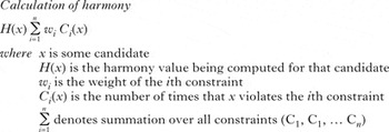
For the present application, the calculation can be made particularly simple if we adopt the idealising assumption that there are only two candidates to consider for each input, one for each value of the harmonising feature. Thus it is implicit in our account that other, non-stated constraints rule out any candidates not mentioned. For example, *[-ndí] for factitive /-ndέ/ can be assigned an arbitrarily low probability by giving Ident[high] an indefinitely high weight.
Once the harmony of the two relevant candidates (Cand1 and Cand2) has been calculated, the probability of Cand1 is determined as in (30).
-
(30)

The probability of Cand2 is 1 minus the probability of Cand1. The overall pattern is that large harmony values (deriving from violations of strong constraints) produce low predicted probability values. The probability predicted for a candidate depends on the aggregate strength of its constraint violations, as well as those of the candidate with which it competes.
6.2 Constraint set
In our analysis of Tommo So, harmony is favoured by markedness constraints of the Agree family (Lombardi Reference Lombardi1999, Baković Reference Baković2000); these are opposed by corresponding faithfulness constraints of the Ident family (McCarthy & Prince Reference McCarthy, Prince, Beckman, Dickey and Urbanczyk1995).Footnote 19 The three Agree constraints are given in (31); these are approximations, whose content is to be modified.
-
(31)
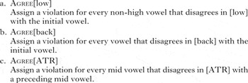
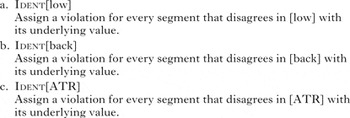
The corresponding Ident constraints are given in (32).
-
(32)
6.3 Scalar constraints
The next step is to modify our Agree constraints so that they are sensitive to the morphologically defined scale in (28). The idea is that when the target disagrees with the trigger vowel in the relevant way, the degree of the violation is determined by the morphological closeness of the target. In particular, following the references cited above, we suggest that the number of violations for any particular Agree constraint is simply the value of the scale for the target vowel. In essence, this turns the calculations of maxent from a multiplication of two values (weights × violations) to a multiplication of three (weights × violations × scalar value), as shown in (33).
-
(33)

The constraints that invoke a scale in our analysis are the Agree constraints of (31); it should now be understood that for each of these constraints, we are scaling the violations according to (28).
6.4 Establishing the weights
As with other stochastic grammar theories, maxent comes with a learning model. It is assumed that the human language learner brings the constraints to the task of acquisition and that the rankings or weights are determined algorithmically during the learner's encounter with language data (see e.g. Tesar & Smolensky Reference Tesar and Smolensky2000, Boersma & Hayes Reference Boersma and Hayes2001 and Boersma & Pater Reference Boersma and Pater2016). We adopt this approach here, using our data corpus as an approximation of real-life learning data.
For maxent grammar, it matters little in practical terms what optimisation algorithm is adopted for purposes of learning; the search space is free of local maxima (Della Pietra et al. Reference Della Pietra, Pietra and Lafferty1997), and many procedures yield essentially the same result. We chose to set the weights to minimise mean absolute error, since this is how we report model fit. For convenience and easy replicability we used the Excel Solver application in its default settings. As a check we recomputed the results with the maxent grammar tool (Wilson & George Reference Wilson and George2009), and obtained very similar results. All weight-setting calculations are posted in the supplementary materials.
We fitted six numbers: the constraint weights for the three Ident constraints and the three Agree constraints. The procedure is non-circular, since we are using six values to predict 20 observations, i.e. the frequency of application for all possible combinations of harmony processes in seven morphological contexts. The weights obtained were as in (34).
-
(34)

6.5 Results
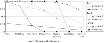
From the grammar thus constructed we computed the predicted percentage of vowel harmony, using the root-closeness values of (28) and the maxent formulae in (30) and (33). These percentages, given in Table IV, closely fit the original data; in fact, the mean absolute error of the maxent model is 0.012 (broken down by harmony type, i.e. Low 0.012, Backness 0.022, ATR 0.000). This compares very favourably with the 0.181 (Low 0.249, Backness 0.134, ATR 0.157) obtained with the inverted exponential model.
Comparison between the observed application rates of harmony (percentages) and the predictions of the maxent grammar. As a high-voweled suffix, the perfective is ineligible for ATR Harmony. If a mid-voweled suffix occurred in this cell, the application rate predicted by the grammar would be zero.

While the superior fit of the model is encouraging, it is also important to understand the model from the viewpoint of restrictiveness – what sorts of frequency patterns could it model in principle? For this purpose it helps to consider in general terms how the model makes its predictions.
6.6 Sigmoid curves and their derivation
Harmonic grammars – in the general case – can be quite complex. Prince (Reference Prince1997) showed that under suitable idealising assumptions, a harmonic grammar can mimic the behaviour of any grammar expressed in Optimality Theory, hence all the intricate data patterns that can be derived with ranking in OT can also be derived in maxent. However, in the present case we have made an additional assumption that greatly simplifies the analysis, namely that all candidates other than simple vowel harmony or the faithful realisation are ruled out by other constraints. Hence only two candidates have any chance of winning, and it is solely the weights of Agree and Ident that determine the outcome.
Simple algebra tells us that under these circumstances, the only frequency patterns that can be derived by the grammar will take the form of sigmoid curves, of the particular type known as the logistic function, widely used in statistical analysis.Footnote 20 The form of the logistic function relating application frequency to morphological distance is given in (35) (it is obtained by substituting (29) and (33) into (30)). In the formula, we generalise from the specific markedness and faithfulness constraints used here to the case of any phonological process governed by a conflicting scalar markedness constraint and non-scalar faithfulness constraint.
-
(35)

Plugging in our particular weights for markedness and faithfulness in (34) into this formula, we can restate Table IV as Fig. 6, plotting the predictions of the analysis as the sigmoid curves generated by the formula. Further mathematics, given in the supplementary materials, demonstrates the restrictiveness of the approach and illuminates the role of the constraint weights in the analysis. The following mathematical results concerning the sigmoid curves are relevant.
Predictions of the maxent grammar plotted as sigmoid curves.

Asymptotes at zero and one. Assuming sufficient room on the horizontal scale, the predicted application rate will asymptote at zero on the low end and one on the high end. Of course, it is possible that the actual values available in the language will not permit us to see these asymptotes; the curves can be ‘cut off’ at one or both ends.
Location of 50% point. The application rate of the phonological process reaches 50% at a point that is determined by the ratio of the constraint weights, specifically at s = wFaith / wMarkedness. For instance, the application rate for Low Harmony crosses 50% on our morphological closeness scale at 5.4 (= 15.2/2.8; for weights see (34)).
Symmetry. The sigmoid curve is symmetrical about the 50% point.
Steepest slope. The steepest slope of the curve occurs at the symmetry point and is determined solely by the weight of the markedness constraint; specifically, it is equal to wMarkedness/4. For instance, in our analysis the essentially categorical cut-off for ATR Harmony is captured with a very high weight (34.8) for Agree[ATR].
We emphasise that these predictions are specific to the Harmonic Grammar model; other theories do not make these predictions, and for them the Tommo So data are correspondingly problematic; either the model fit is bad, as with the inverted exponentials discussed in §5, or the theory is not restrictive enough and can fit essentially any data (see §7).
We can now justify an assertion made earlier in connection with our root-closeness scale (28): it does not matter what we pick as the baseline value or interval size. As (35) suggests, different choices made for the root-closeness scale are cancelled out when the best-fit weights are found. Thus, if we made the interval size of our scale 2 instead of 1, the best-fit model would use a value for wAgree that was half as big. More generally, the expression wFaith − wMarkednesss in (35) represents a linear rescaling (y = mx + b) of s, meaning that appropriate choices of weights exist that can compensate for any linear rescaling of (28).
6.7 A variant with Noisy Harmonic Grammar
We have expressed our account in maxent, but this is not the only framework for stochastic analysis in Harmonic Grammar. In Noisy Harmonic Grammar (Boersma & Pater Reference Boersma and Pater2016), a ‘noise’ factor drawn from the Gaussian distribution is added to the weight of each constraint every time the grammar is applied, and the output for any given input for that particular application is simply the most harmonic candidate. The probabilities of the candidates in the general case are defined as the probability distribution over multiple applications. The best-fit constraint weights can be calculated in various ways. Mathematically, Noisy Harmonic Grammar generates symmetrical zero-to-one sigmoid curves, just like maxent, but the sigmoids are from a different function (the cumulative normal distribution), which is strikingly similar visually to the logistic function employed by maxent.
Noisy Harmonic Grammar turned out to work slightly better than maxent, with a mean absolute error of 0.009 (cf. maxent 0.012). Errors for each harmony process are: Low 0.005, Backness 0.021, ATR 0.000.
A technical issue in Noisy Harmonic Grammar is how the noise should be added in the case of scalar constraints: in principle it could be added before the harmony contribution is multiplied by the scale value, so that noise itself is multiplied. This produces asymmetrical sigmoids and indeed a slightly worse model fit (mean absolute error 0.031). The value 0.009 just mentioned is obtained by adding the noise after multiplication.Footnote 21
6.8 Analysing the English -t,d-deletion data in maxent
It is appropriate to ask whether the English -t,d-deletion data that motivated Guy's inverted exponential theory can be modelled under our theory. The answer is that it can. In brief, we set up a -t,d-deletion model employing the weighted constraints *CT (which penalises clusters; w = 0.69) and Max(T) (faithfulness; w = 1.01), with the root-closeness scale 3 = root, 2 = Level 1, 1 = Level 2. For Santa Ana's (Reference Santa Ana1991) data this gives highly accurate results.Footnote 22
6.9 Sigmoid curves in linguistic theory
Sigmoids have provided good data fit in various places in linguistics whenever a constraint with scalar violations stacks up against a constraint with constant violations. Albright (Reference Albright2012), in a study of phonotactics, finds that variable phonotactic disharmony scores get a closer fit to lexical frequency when pitted against the non-scalar constraint MParse. In McClelland & Vander Wyk's (Reference McClelland and Vander Wyk2006) study of interacting phonotactic constraints in English, a term β, analogous in effect to Albright's MParse, also improves model fit. Earlier, Frisch et al. (Reference Frisch, Broe and Pierrehumbert1997) used a constant term K pitted against a scalar constraint in order to derive logistic curves predicting the frequency of consonant pairs in Arabic roots from their similarity. Zuraw (Reference Zuraw2012), studying morphophonemic nasal mutation in Tagalog, finds that the Tagalog prefixes differ in their propensity to trigger nasal mutation, and stem-initial consonants differ in their propensity to undergo it; each prefix gives rise to its own sigmoid curve. Much earlier, Kroch (Reference Kroch1989) presented a model in which a syntactic constraint rises in weight over time, overtaking a set of opposed statically weighted constraints, and thus creating a family of diachronic sigmoids; the model matches well with Kroch's diachronic data. For further discussion see Zuraw (Reference Zuraw, Bod, Hay and Jannedy2003).
7 Two non-restrictive approaches
We have thus far considered two models that work well in accounting for the Tommo So data (maxent, Noisy Harmonic Grammar), and also some models that work poorly (inverted exponentials and the stripped-down constraint sets of note 28). Here we critique two models that fit the Tommo So data perfectly, but at great cost in restrictiveness.
7.1 Morpheme indexation
It is likely that there are phonological processes triggered by specific morphemes or undergone by specific morphemes. Pater (Reference Pater2000, Reference Pater and Parker2009b) suggests that particular markedness or faithfulness constraints can be indexed to particular morphemes. Work supporting this view includes Flack (Reference Flack2007), Gouskova (Reference Gouskova2007), Steriade (Reference Steriade, Bachrach and Nevins2008), Jurgec (Reference Jurgec2010) and Linzen et al. (Reference Linzen, Kasyanenko and Gouskova2013).
We have found that if we affiliate a separate Agree constraint with each affix of Tommo So (along with one for roots), we can achieve a very good – indeed, perfect – fit to the data. For instance, we factored our system of Agree constraints to include 21 constraints in total – one for each combination of morphological type and harmony process; e.g. Agree[back]factitive. Coupled with our three Ident constraints in (32) and implemented in maxent, this achieves an essentially perfect data fit (mean error 0.00000064).
As a reviewer points out, this ‘would be a less restrictive model … since there would be no predicted connection between linear order of morphemes and frequency of alternation’. Indeed, the model is the least restrictive conceivable. No matter what data we gave it, constraint weights could be found that achieve a perfect fit.
A specific consequence is that morpheme indexation does nothing to explicate the essential Kiparskian generalisation that application frequency diminishes in outer morphological layers. We think our approach is a better theory, because it actually predicts this pattern. It remains a problem to explain why morpheme-specific markedness or faithfulness constraints do not commonly subvert the Kiparskian pattern; perhaps these constraints represent something of a ‘last-resort’ option of language learners, invoked only when more natural constraints cannot account for the data.
7.2 Domain-indexed constraints following a stringency hierarchy
A similar approach indexes constraints to morphological domains rather than individual morphemes. Kiparsky (Reference Kiparsky1994), reanalysing the English -t,d-deletion pattern in §5, uses a model of this sort. The key idea is that ‘a violation at any given level is necessarily a violation at all superordinate levels (but not conversely).’ Applied to /t/-deletion, the pattern would look like (36). Such a pattern is a stringency hierarchy (Prince Reference Prince1997, de Lacy Reference de Lacy2004) and may be related to the Strong Domain Hypothesis of Lexical Phonology (Kiparsky Reference Kiparsky, Elert, Johansson and Strangert1984, Myers Reference Myers1991; rules may ‘turn off’ at later levels but not ‘turn on’).
-
(36)
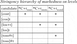
Kiparsky stipulated that the ranking probability between each indexed markedness constraint and the opposing faithfulness constraints must be exactly the same. With this condition, the theory makes exactly the same predictions as the rule-based approach of Guy that inspired it. In particular, it works well for the English -t,d-deletion data – but by the same token, it fails badly when applied to Tommo So.
On the other hand, as a reviewer suggested, the approach might be adapted to Tommo So by abandoning the assumption that the ranking probability with respect to faithfulness must remain the same for each constraint in the stringency hierarchy. Pursuing this suggestion, we set up a hierarchy for the Tommo So Agree constraints, illustrated here for Backness Harmony; forms are taken from §4.
-
(37)
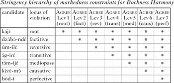
The domain-indexation model behaves similarly to the morpheme-indexation model just discussed: when coupled with a stochastic grammar framework, it can provide an exact match to the Tommo So data pattern. Moreover, unlike morpheme indexation, domain indexation at least does cover the central generalisation that application frequency descends going outward from the stem.Footnote 23 However, it also suffers from insufficient restrictiveness, as it can derive any non-ascending quantitative pattern.Footnote 24 For instance, it can derive patterns that descend in a straight line, or that asymptote at values other than one or zero (e.g. starting or ending with a level sequence at 0.5); for graphical demonstrations see the supplementary materials. In contrast, our scalar model is tightly constrained by the mathematical generalisations given in §6.6; it generates only symmetrical descending curves that asymptote at one and zero.
7.3 Summary and evaluation of all models
In this article, we have considered multiple models to account for the Tommo So vowel-harmony data. By far the most successful were those based on scalar constraints and Harmonic Grammar. Both the maxent and Noisy Harmonic Grammar versions achieved a close fit to the data. Poor fits, on the other hand, were obtained under a number of different approaches. The inverted-exponential model (§5) was one such case, whether or not an intercept term is included (note 22). Our own Harmonic Grammar models also performed poorly if we attempted to simplify them by removing the possibility of language-specific weights for either faithfulness or markedness (note 22). Lastly, both the morpheme-indexation approach (§7.1) and domain indexation with stringency (§7.2) fit the data perfectly, but in a sense they are uninteresting, because they can fit either any data pattern whatsoever (morpheme indexation) or any descending pattern (domain indexation). Table V summarises, giving error values for each model.
Summary of models of the Tommo So vowel-harmony data.

8 Further issues
8.1 What kind of variation?
Variation in phonology takes several forms. For instance, it can be either interspeaker or intraspeaker variation. In the former case, every speaker always produces the same outputs, and the appearance of variation in the data as a whole is merely the result of mixing in data from different speakers. We think the variation we describe here is intraspeaker variation; there is no independent evidence of dialect differences among the language consultants, and the collected data include numerous instances in which the same speaker said the same word on different occasions with different harmony; see e.g. (9), (10) and (19).
Intraspeaker variation involves either types or tokens. In type variation, words or stems of similar phonological make-up behave differently on an idiosyncratic, lexically determined basis, but each one is always pronounced the same. In token variation, all words or roots that are phonologically eligible for variation vary from one speaking occasion to the next. In light of our observations, Tommo So cannot be a case of pure type variation, but it is possible that some words are lexically listed (or diacritically marked) as always having harmony or non-harmony. Such forms are difficult to detect in our data, and the results of the following statistical inquiry are inconclusive.
Test 1. One way of testing for the presence of listed forms is to check whether there are more all-harmony and no-harmony words among the population of varying forms than could arise by chance. We tested this with a Monte Carlo simulation (Mooney Reference Mooney1997). In our corpus there are 155 types that have a combination of root + suffix with a harmony rate above zero and below one, and with more than one attested token; these are the types in which token variation can, in principle, be detected. The total number of tokens of these types is 723. To execute one single Monte Carlo run on one single token, we toss a simulated biased coin whose probability of heads is equal to the theoretical probability of harmony, taken from Table III. Recording this outcome, we repeat the process for all 723 tokens. Examining the batch of pseudo-data thus created, we count the number of types whose tokens come out all-harmony, and the number of types that come out no-harmony. The whole process is repeated 100,000 times, yielding an approximate probability distribution for the expected number of all-harmony and no-harmony types. Lastly, we examine where the real counts (66 no-harmony, 48 all-harmony) fall in this distribution. The total fraction of Monte Carlo trials that have 66 or more no-harmony forms, or 48 or more all-harmony forms, divided by 100,000, yields a p-value, telling us the probability that these numbers could arise by chance. The results are highly significant: p < 0.00001 in both cases. In other words, our test shows that there are far more all-harmony and no-harmony cases then could ever arise by chance.
In principle, this could be taken as evidence that there is substantial type variation, in the form of root + suffix combinations that are memorised in some way. However, the picture is not so clear. Our experience in elicitation suggests that consultants are vulnerable to self-priming: if they give one possible free-variation outcome then the odds are good that they will give the same one when asked a few minutes later. Under the self-priming effect, we might expect a statistically significant effect in the test just given, even if Tommo So words are not listed with their harmony outcomes.
Moreover, if there are type effects in our data, it is strikingly hard to locate the individual words that are responsible. This is what we found in Test 2.
Test 2. The goal is to find the words that display a great deal or very little harmony in the context of the overall probability predicted for them by our analysis. To do this, we consult the cumulative binomial distribution for (at least/fewer than) m harmony outcomes when there are n tokens (Mosteller et al. Reference Mosteller, Rourke and Thomas1970: 138–145). In fact, very few words pass this test, even with a liberal 5% significance criterion.Footnote 25 One such example is /dùló-íjέ/ (turn around-mediopass) ‘return’, which appears eight times in the corpus as [dùlíjó] and never as [dùlíjé]. The probability of Backness Harmony in the mediopassive is 0.44; hence the probability of unanimity for [dùlíjó] is 0.448, or 0.0014; this is unlikely to be accidental.
Curiously, all nine words that pass this test at the 0.01 significance level (such as [dùlíjó]) are words with invariant harmony. To explain this, we suggest that these words have been restructured and are treated synchronically as roots (which in Tommo So virtually always undergo harmony; §4.1). A possible English analogue (Kiparsky Reference Kiparsky1977: 222) is the exceptional compound high school [ˈhʌɪ skul], treated as a single stem and thus eligible for the raising process /aɪ/→[ʌɪ] /__[−voice]; the normal outcome is seen in pie school [ˈpaɪ skul].
Obviously, more data would be needed to make further progress on the type/token question. For now, we think the best conjecture is that type variation may play a quite small role: we cannot prove that the overall disparities (Test 1) are not due merely to self-priming, and the very few cases where the type variation is clearly localisable to particular words (Test 2) share the all-harmony property, suggesting that the only mechanism at play is the treatment of a small number of historically polymorphemic words as monomorphemic.
8.2 Opacity with Hiatus Resolution
ATR Harmony in Tommo So is opaque: it is in a counterbleeding relationship with Hiatus Resolution. In roots with an initial high vowel and a final mid vowel, the only possible ATR trigger is the final vowel, since only mid vowels may trigger ATR Harmony (§4.4). When a vowel-initial suffix is added to such a root, this final vowel deletes, yet the suffix vowel agrees in [ATR] as though it were present, as shown in (38).
-
(38)

As these examples show, the suffix's [ATR] value is determined by a vowel no longer present on the surface. In a rule-based analysis, this result would be obtained by ordering ATR Harmony before Hiatus Resolution.
In constraint-based phonology, there are several theories that would permit the derivation of these opaque cases. Employing autosegmental theory, we could let vowel deletion strand a floating Root node (Clements Reference Clements1985). Provided that this node is visible to the Agree constraints, opacity would result. Opacity could also be obtained by framing our analysis within various standard approaches within OT: Sympathy Theory (McCarthy Reference McCarthy1999), Turbidity Theory (Goldrick Reference Goldrick2000), Stratal OT (Bermúdez-Otero Reference Bermúdez-Otero1999, Kiparsky Reference Kiparsky2000, Reference Kiparsky, Féry and van de Vijver2003), Candidate Chain Theory (McCarthy Reference McCarthy2007). Since the analysis of opacity is tangential to our main concerns, we will not explore the matter further.
9 Conclusion
We list what we take to be the main results of this work.
First, Tommo So vowel harmony is a clear case of the Kiparskian generalisation that phonological processes ‘turn off’ as they extend into the outer reaches of morphology. With a rich set of ordered affixes, Tommo So forms a test case for formal theories that seek to account for this phenomenon.
Second, Guy's inverted-exponential theory, though simple and principled, does not provide a good fit to the Tommo So data. Other models of phonology–morphology interactions, namely morpheme-indexed constraints and domain-indexed constraints with a stringency hierarchy, are able to provide an essentially perfect match, but this result is uninformative because these models are unrestrictive.
Third, Harmonic Grammars (both maxent and Noisy Harmonic Grammar), augmented to include scalar constraints, provide a good fit to our data. Moreover, these theories are restrictive; they inherently generate sigmoid probability functions and can only be used to model curves that fit this family.
This said, we judge that our work remains speculative until a greater number of ‘petering out’ systems have been located and documented with enough data to do quantitative analysis. We hope the method described here will facilitate the task of taking on new cases.