2. The pension model

We consider a DB pension plan of aggregated type with continuous entrance and retirement of members in such a way that the pension population remains stable at every time. Active participants coexist with retired participants at every time. It is supposed that every participant enters the plan at the same age l and retires at age l ^′, that is, she remains $l'-l$ years. Since this takes place along time, we need to consider both the time elapsed since the plan started and the age of the participants. The benefits promised to the workers at the age of retirement are established in advance by the manager and are directly related with the salary. At each instant of time t, the benefits of the departing members, with age l ^′, and the contributions of the members, with age between l and l ^′, are accumulated, because the plan is aggregated. The pension fund has a finite planning horizon T. This final time can be thought of as the time at which some additional, and known in advance, uncertainty will affect the plan as for instance the transition to a new plan. This fact is interiorized by the fund manager by discounting the utility from the fund wealth at T at higher rate of time preference than the applied to instantaneous utilities obtained along the time horizon. Workers not retired at this final date receive compensation from the surplus obtained in the process of management of the fund assets.

The principal elements intervening in the funding process and the essential hypotheses allowing its temporary evolution to be determined are as follows. The value of fund assets at time t is denoted by F(t). The benefit promised to the participants at time t is B(t) and is a percentage of the total salary of the workers at the moment t. C(t) is the contribution rate made by the sponsor at time t to the funding process. The total salary of the plan members at time t is denoted by s(t) and is a stochastic process correlated with the financial market. u(t) is the percentage of salary contributed to plan at time t. To avoid confusion of u(t) with the contribution rates, we will refer to C(t) as simply contributions. The constant discount rate associated with the instantaneous utility is $\rho_1,$ and the constant discount rate associated with the final utility is $\rho_2$ .

In order to ensure the standard of living of the participants, the manager of the pension plan assumes that benefit and rate of contribution are related with salary. We suppose that the benefit and the contribution are proportional to the total salary,

(2.1) \begin{align} B(t)=&\,k s(t), \end{align}

(2.2) \begin{align}C(t)= &\,u(t) s(t) ,\end{align}

where the constant k is positive and $k\geq u(t)$ for every $t\in[0,T]$ .

The difference between benefit and contribution is the net benefit. From (2.1) and (2.2), it can be obtained as

(2.3) \begin{equation} B(t)-C(t)= (k-u(t))s(t).\end{equation}

Note that the explicit appearance of the salary constitutes a novelty compared with the model in Josa-Fombellida and Rincón-Zapatero (Reference Josa-Fombellida and Rincón-Zapatero2004), which studies a dynamic mathematical model for a stochastic DB pension plan. While the relationship between the actuarial functions is maintained, now a spread method of amortization is not longer used. See Remark 5.2 in Josa-Fombellida and Rincón-Zapatero (Reference Josa-Fombellida, López-Casado and Rincón-Zapatero2008a).

2.1. The financial market, the salary process and the fund wealth

In this section, we describe the financial market where the fund operates and the salary process. The randomness involved in the financial market is given by the standard Brownian motion n-dimensional, $z=(z_{1},\ldots,z_{n})^{\top}$ , where ${}^{\top}$ denotes transposition. We assume the total salary is a stochastic process built from the d-dimensional Brownian motion $w=\left(w_{1},\ldots,w_{d}\right)^{\top}$ and influenced by the financial market. We consider the complete probability space $(\Omega,\mathcal{F},\mathrm{P})$ , generated by z ad w, that is to say, $\mathcal{F}$ is the filtration containing the information available to the sponsor plan, $\left\{ \mathcal{F}_{t}\right\}_{t\in[0,T]},$ with $\mathcal{F}_{t}=\sigma\! \left\{(z(\nu) ,w(\nu));\,0\leq \nu\leq t\right\}.$

The financial market consists of a portfolio with n risky assets $\left\{ P^{i}\right\} _{i=1}^{n}$ , which are correlated GBMs generated by z, and a riskless asset $P^{0}$ , whose evolution, as proposed in Merton (Reference Merton1971), is given by

(2.4) \begin{align}dP^{0}(t) &=rP^{0}(t)dt,\quad \text{with }r>0, \qquad\qquad\qquad\qquad\qquad\qquad\qquad\quad\end{align}

(2.5) \begin{align}dP^{i}(t) &=P^{i}(t)\left( \mu_{i}dt+\sum_{j=1}^{n}\sigma_{ij}dz_{j}(t)\right), \quad \text{with }\mu_{i}>0,\quad i=1,2,...,n, \end{align}

where $r>0$ is the risk-free rate of interest, $\mu_i$ the mean rate of return of the risky asset $P^i$ , and $\sigma_{ij}$ its volatility or uncertainty parameters. We assume that $\mu_{i}>r$ for all i, so the manager has incentives to invest with risk. The amount of fund invested at time t in the risky asset $P^{i}$ is denoted by $\lambda_{i}(t)$ , $i= 1,2,\ldots,n$ . The remainder, $F(t)-\sum_{i=1}^{n}\lambda_{i}(t)$ , is invested in the bond. Borrowing and short selling is allowed. A negative value of $\lambda_{i}$ means that the sponsor sells a part of his risky asset $S^{i}$ short while, if $\sum_{i=1}^{n}\lambda_{i}$ is larger than F, he or she then gets into debt to purchase the stocks, borrowing at rate of interest r.

We suppose $\{\boldsymbol{\Lambda}(t)\,:\, t\geq0\}$ , with $\boldsymbol{\Lambda}(t) = (\lambda_{1}(t), \lambda_{2}(t),\ldots,\lambda_{n}(t))^{\top}$ , is a control process adapted to the filtration $\{\mathcal{F}_{t}\}_{t\ge 0}$ , $\mathcal{F}_{t}$ -measurable, Markovian and stationary, satisfying

(2.6) \begin{equation} \int_{0}^{T}\boldsymbol{\Lambda}(t)^{\top}\boldsymbol{\Lambda}(t)dt<\infty,\,\, \mathrm{P}\text{-a.s.,}\end{equation}

and the contribution relative to salary, u, is a non-negative measurable adapted process with respect to $\left\{\mathcal{F}_{t}\right\}$ satisfying

(2.7) \begin{equation} \int_0^T u(t) s(t) dt <\infty,\,\, \mathrm{P}\text{-a.s.}\end{equation}

The salary process is given by the general stochastic differential equation (SDE)

(2.8) \begin{equation} d s(t)=\eta(s(t)) dt +\sum_{j=1}^n \beta_{j}(s(t)) dz_j(t)+\sum_{j=n+1}^{n+d} \beta_{j}(s(t)) d w_{j-n}(t),\end{equation}

with initial conditions $s(0)= s_0>0$ , and where $\eta(s)$ is the mean rate of growth of the salary s, and $\beta(s)$ its volatility. We assume $s>0$ a.s. This is satisfied if the salary is a GBM as in Section 4. Note that Brownian motion z also appears in expression (2.8) because the salary is correlated with the financial market.

The manager uses the contribution to increase the fund wealth. The fund not devoted to the net benefit is invested in the financial market. Therefore, the fund’s dynamic evolution under the investment policy $\boldsymbol{\Lambda}$ is:

(2.9) \begin{equation} dF(t)=\sum_{i=1}^{n}\lambda_i(t)\frac{dP^{i}(t)}{P^{i}(t)} + \left(F(t)-\sum_{i=1}^{n}\lambda _{i}(t)\right) \frac{dP^0(t)}{P^0(t)} +(C(t)-B(t))\, dt,\end{equation}

with the initial condition $\,F(0)=F_0>0$ . By substituting (2.3), (2.4) and (2.5) in (2.9), we obtain:

(2.10) \begin{equation}dF(t) = \left( rF(t)+\sum_{i=1}^{n}\lambda_i(t)(\mu-r)+ (u(t)-k)s(t)\right) dt + \sum_{i=1}^{n}\sum_{j=1}^{n}\lambda_i(t) \sigma_{ij}\,dz_{j}(t),\end{equation}

that, with the initial condition and (2.8), determines the fund evolution. We assume the notation: $\boldsymbol{\mu}=(\mu_{1},\mu_{2},\ldots,\mu_{n})^{\top}$ , $\textbf{1} =(1,1,\ldots,1)^{\top}$ , $\sigma=(\sigma_{ij})$ and $\Sigma=\sigma\sigma^{\top}$ . We suppose the existence of $\Sigma^{-1}$ , that is, the existence of $\sigma^{-1}$ . The market price of risk is denoted by $\boldsymbol{\theta}=\sigma^{-1}\!\left(\boldsymbol{\mu}-r\textbf{1}\right).$ Finally, in matrix notation, the diffusion term of the salary process is $\beta(s)=(\beta^{z}(s)\,|\, \beta^{w} (s))$ , with $\beta^{z}(s)=(\beta_{j})_{j=1,\ldots,n}$ and $\beta^{w}(s)=(\beta_{j})_{j=n+1,\ldots,n+d}$ row vectors.

The fund and the salary processes, (2.10) and (2.8), in vectorial notation are

(2.11) \begin{align} dF(t)= \left(rF(t)+\boldsymbol{\Lambda}^{\top}(t)(\boldsymbol{\mu}-r\textbf{1})+(u-k) s(t)\right)dt +\boldsymbol{\Lambda}^{\top}(t)\sigma dz(t),\end{align}

(2.12) \begin{align} d s(t)=& \eta(s(t)) dt + \beta^{z}(s(t)) dz(t) +\beta^{w}(s(t)) dw(t), \end{align}

with initial condition $(F_0, s_0)$ .

2.2. The optimization problem

In the following, we will consider the new control variable $v(t)=(k-u(t)) s(t)$ , which is the liquid or net benefit for the participants at time t. The plan manager wishes to minimize the contributions or equivalently the relative contribution payments u, in [0, T]. Following the idea of Berkelaar and Kouwenberg (Reference Berkelaar and Kouwenberg2003) for a retirement-saving model for a single individual, and later Josa-Fombellida and Rincón-Zapatero (Reference Josa-Fombellida, López-Casado and Rincón-Zapatero2008a) and Chen and Hao (Reference Chen and Hao2013) for a pension plan manager, we suppose that higher contributions payments decrease the utility of the manager and increase the marginal utility of reduction in payments. Thus, it is minimizing the possibility that an increase in the contribution rates will probably lead to the plan manager to pay the workers higher salaries in order to hire them originally or to keep them. On the other hand, the pension plan is more attractive for the workers by the aim of minimize contributions.

We suppose that higher contribution payments decrease the utility of the manager and increase the marginal utility of reduction in payments. Hence, the running utility function, $U(v/s)$ , is increasing and concave with respect to the liquid benefit relative to salary, $v/s=k-u;$ thus, a higher relative contribution implies lower utility. Additionally, the sponsor’s goal is to maximize the same increasing and concave utility function, U, of the final level at fund assets relative to the salary s, $U(F/s)$ . The CRRA (constant relative risk averse) utility functions, namely the logarithmic and power functions and the exponential CARA (constant absolute risk averse) utility function, are suitable for the purposes of the manager and allow explicit solutions. Power and logarithmic utility functions make that $B-C=(k-u)s>0;$ therefore, the risk is transferred to the evolution of the fund. Thus, the model is established for not shifting the risk to the employees but the fund evolution could be with moderate or bearish growth, depending on the financial market, and as a consequence, the manager may have an unsatisfactory low level of the fund on the end date of the plan.

Given initial values of time, $t_0$ , fund assets, $F_0$ , and salary, $s_0$ , we denote by ${\mathcal{A}}_{t_0,F_0,s_0}$ the class of admissible controls, that is to say, the set of measurable processes $(u,\boldsymbol{\Lambda})$ satisfying (2.6) and (2.7), and where F and s satisfy (2.11) and (2.12), respectively. The objective functional to be maximized over the class of admissible controls, ${\mathcal{A}}_{t_0,F_0,s_0}$ , is given by

(2.13) \begin{align} J((t_0,F_0,s_0);\, (v,\boldsymbol{\Lambda}))= \mathbb{E}_{t_0,F_0,s_0}\left\{\int_{t_0}^{T } e^{-\rho_1(t-t_0)}\,U\left(\frac{v(t)}{s(t)}\right)\,dt+ e^{-\rho_2(T-t_0)} \alpha U\left(\frac{F(T)}{s(T)}\right)\right\},\end{align}

where $\mathbb{E}_{t_0,F_0,s_0}$ denotes conditional expectation with respect to the initial conditions $(t_0, F_0,s_0)$ , and $\alpha>0$ is a weighting factor indicating the importance of maximizing the final utility. The imposed admissibility conditions, (2.6) and (2.7), guarantee that the system of SDEs defining the fund, (2.11) and (2.12), has a unique solution for each initial value of the fund and of the salary.

By the so-called heterogeneous discounting, in expression (2.13), the manager discounts differently the instantaneous utility over the planning horizon and the final utility captured by the final function. Under the assumption that $\rho_2>\rho_1$ , two effects arise from this setting. The first is that now the manager’s time preferences become time-inconsistent, in the sense that they will be different at different instants of time along the planning horizon $[t_0,T]$ . Because of this, standard dynamic optimization techniques fail to characterize time-consistent solutions, and it is necessary to adapt the usual dynamic programming equation in the search of time-consistent solutions (see, e.g., Marín-Solano and Patxot, Reference Marín-Solano and Patxot2012 for the deterministic problem, or de-Paz et al., Reference de-Paz, Marín-Solano and Navas2013 for the stochastic case). In this context, with the term “time-consistent” we refer to the usual meaning in the sense that, for a given planning horizon $[t_0,T]$ , if at any time $t'>t$ , $t'\in (t,T]$ , the decision maker decides to reoptimize and solves the truncated problem from t ^′ until the end of the planning horizon T, taking as initial conditions for the state variables their values at t ^′ resulting from strategies applied over [t, t ^′], the new solution will coincide with the one initially computed at time t for [t ^′, T]. Because of this, the decision maker will have no incentives to deviate from the original strategies. In fact, what we are obtaining is the Markov Perfect equilibrium (MPE) between the current manager, the manager with time preferences at moment t or t-agent, and her future selves, the t ^′-agents, with $t'\in (t,T]$ for any $t\in [t_0,T]$ (see, e.g., Karp, Reference Karp2007), who decide optimally for an infinitesimal amount of time. In this sense, when alluding to the obtained controls, from a formal point of view they should just be named time-consistent strategies, as there is not a unique decision maker for whom the solution is optimal but an infinite number of them, one for any instant of time, that is, we characterize the MPE for the constrained (sequential game) problem between the t-agent and her future selves.

The other effect, which is specific to the heterogeneous discounting model and a consequence of the assumption that $\rho_2>\rho_1$ , is that the relative valuation of the final function increases as we approach the end of the planning horizon. This can be easily seen by rewriting the final function at (2.13) as

\begin{equation*}e^{-\rho_1 (T-t)} e^{-(\rho_2-\rho_1)(T-t)} U(F(T)/s(T))\end{equation*}

for $t\in[t_0,T]$ . Note that now, the problem can be interpreted as a problem with standard discounting (at rate $\rho_1$ ), but with a modified final function equal to $e^{-(\rho_2-\rho_1)(T-t)}U(F(T)/s(T))$ . It is clear that, abstracting from the standard discount at rate $\rho_1$ , an t ^′-agent will give a higher valuation to an additional utility unit than the one given by a t-agent, as long as $t'>t$ . Moreover, this valuation is increasing the closer to T the t ^′-agent is (note that under the assumption of $\rho_2<\rho_1$ the effect would be the contrary).

The dynamic programming approach is used to solve the problem. The value function is defined as

\begin{equation*}\widehat{V}(t,F,s) =\max_{(v,\boldsymbol{\Lambda})\in {\mathcal{A}}_{t,F,s}}\big\{ J((t,F,s);\,(v,\boldsymbol{\Lambda})) \,|\, \mbox{ s.t. }(2.11),(2.12)\big\}.\end{equation*}

The connection between value functions and time-consistent feedback strategies in stochastic control theory with heterogeneous discount is accomplished by a modified Hamilton-Jacobi-Bellman (HJB) equation; see Corollary 1 in de-Paz et al. (Reference de-Paz, Marín-Solano and Navas2013) and Proposition 1 in de-Paz et al. (Reference de-Paz, Marín-Solano, Navas and Roch2014). The value function $\widehat{V}$ satisfies the modified HJB equation

(2.14) \begin{align}-\rho_2 V & +K+V_t+ \max_{v,\boldsymbol{\Lambda}}\!\left\{U\left(\frac{v}{s}\right)+ \left(rF +\boldsymbol{\Lambda}^{\top}(\boldsymbol{\mu}- r\textbf{1})-v\right) V_{F}+\eta V_s\right.\nonumber\\[5pt]& \left.+ \frac{1}{2} \boldsymbol{\Lambda}^{\top}\Sigma\boldsymbol{\Lambda}V_{FF}+ \boldsymbol{\Lambda}^{\top} \sigma(\beta^z)^{\top} V_{Fs}+\frac{1}{2} \mathop{\rm tr}\nolimits\left\{\beta\beta^{\top}V_{ss}\right\} \right\}=0, \end{align}

where K(t, F, s) solves the auxiliary PDE

(2.15) \begin{align}\nonumber-\rho_1 K+K_t\,+\, &(\rho_2-\rho_1)U\left(\frac{\widehat{v}}{s}\right)+ \left(rF+\widehat{\boldsymbol{\Lambda}}^{\top}(\boldsymbol{\mu}- r\textbf{1})-\widehat{v}\right) K_{F}+\eta K_s\\[5pt]&\quad + \frac{1}{2} \widehat{\boldsymbol{\Lambda}}^{\top}\Sigma\widehat{\boldsymbol{\Lambda}} K_{FF}+ \widehat{\boldsymbol{\Lambda}}^{\top}\sigma (\beta^z)^{\top} K_{Fs}+\frac{1}{2} \mathop{\rm tr}\nolimits\left\{\beta\beta^{\top}K_{ss}\right\}=0, \end{align}

where $\widehat{v},\widehat{\boldsymbol{\Lambda}}$ are the arguments maximizing in (2.14). The final conditions are $V(T,F,s)=\alpha U(F/s)$ and $K(T,F,s)=0$ , for all F, s.

Remark 2.1. The model considers that the benefits and the contributions are indexed by the salary process. Thus, we assume the modeling approach in Josa-Fombellida and Rincón-Zapatero (Reference Josa-Fombellida, López-Casado and Rincón-Zapatero2008a), but only considering one group of workers, in order to facilitate the development. An alternative model could be considered, as further research, without taking into account the salary, but considering a specification for the benefit as a geometric Brownian motion, as in Josa-Fombellida and Rincón-Zapatero (Reference Josa-Fombellida and Rincón-Zapatero2004). Then, other actuarial elements, such as the actuarial liability AL, could be included in the model. The heterogeneous discount would appear in the objective functional as follows

\begin{align*}& J((t_0,F_0,AL_0);\, (v,\boldsymbol{\Lambda}))= \mathbb{E}_{t_0,F_0,\mbox{{A L}}_0}\left\{\int_{t_0}^{T} e^{-\rho_1(t-t_0)}\,U\!\left(B(t)-C(t)\right)\,dt+ e^{-\rho_2(T-t_0)}\alpha U\left(F(T)\right)\right\}.\end{align*}

3. The time-consistent strategies

In this section, we analyze how the manager may select the time-consistent relative contribution rate and the investment strategies of the fund put into the risky assets, as well as some properties of these policies.

Though explicit solutions could be obtained with several utility functions such as the exponential CARA utility function, we consider a power CRRA utility function as in Josa-Fombellida and Rincón-Zapatero (Reference Josa-Fombellida, López-Casado and Rincón-Zapatero2008a) and in Josa-Fombellida et al. (Reference Josa-Fombellida and Rincón-Zapatero2018).

When $\gamma=1,$ we consider the logarithmic utility, $U(x)=\ln x$ . The parameter $\gamma$ is the risk aversion. The manager has high-risk aversion for $\gamma>1$ , moderate for $\gamma=1$ and low for $\gamma<1$ .

We have the following result:

Theorem 3.1. Suppose that Assumption A holds. Then, the time-consistent relative contribution rate and the investments in the risky assets are given by

(3.1) \begin{align} u(t,F,s)&= k - s^{-\frac{1}{\gamma}} {g^{-\frac{1}{\gamma}}(t,s)} F,\qquad\qquad\qquad\qquad\qquad \end{align}

(3.2) \begin{align} \Lambda(t,F,s)&= \frac{1}{\gamma}\left ( \Sigma^{-1} (\boldsymbol{\mu}-r \textbf{1})+\frac{g_{s}(t,s)}{g(t,s)} \sigma^{-\top} (\beta^{z}(s))^{\top}\right)\! F \end{align}

respectively, where $g\,:\,[0,T] \times \mathbb{R}^n \longrightarrow \mathbb{R}$ is a positive solution of the non-linear system of PDEs (partial differential equations)

(3.3) \begin{align}g_t(t,s) & + h(t,s) + \left(-\rho_2 + r(1-\gamma) -\frac{1}{2}\left(1-\frac{1}{\gamma}\right)\boldsymbol{\theta}^{\top} \boldsymbol{\theta} \right ) g(t,s)\nonumber\\[5pt] & + \left(-\left(1-\frac{1}{\gamma}\right)\beta^z(s)\boldsymbol{\theta} +\eta(s)\right) g_s(t,s)+\gamma s^{1-\frac{1}{\gamma}} {g^{1-\frac{1}{\gamma}}(t,s)}\\[5pt] & -\frac{1}{2}\left(1-\frac{1}{\gamma}\right)\frac{{g_s^2(t,s)}}{g(t,s)} \beta^{z}(s)(\beta^{z}(s))^{\top}+\frac{1}{2} \mathop{\rm tr}\nolimits\! \left\{ \beta(s)\beta(s)^{\top}\right\} g_{ss}(t,s)=0, g(T,s) = \alpha s^{-(1-\gamma)},\nonumber \end{align}

(3.4) \begin{align} h_t(t,s) &\, +\left( -\rho_1 +r(1-\gamma) -\frac12 \left(1-\frac{1}{\gamma}\right) \boldsymbol{\theta}^{\top}\boldsymbol{\theta}\right.\qquad\qquad\qquad\qquad\qquad\qquad\qquad\qquad \qquad \nonumber\\[5pt]& \left. +\frac{1}{2} \left(1-\frac{1}{\gamma}\right)\beta^z(s) \beta^z(s)^{\top}{\frac{g_s^2(t,s)}{g^2(t,s)}} - (1-\gamma)s^{1-\frac1\gamma}{g^{-\frac1\gamma}(t,s)} \right) h(t,s)\nonumber\\[5pt] & \,+(\rho_2-\rho_1) s^{1-\frac{1}{\gamma}}{g^{1-\frac{1}{\gamma}}(t,s)}+ \left(\eta(s)-\left(1-\frac{1}{\gamma}\right)\beta^{z}(s)\boldsymbol{\theta}\right.\nonumber\\[5pt]& \left. -\left(1-\frac{1}{\gamma}\right)\beta^z(s)\beta^z(s)^{\top} \frac{g_s(t,s)}{g(t,s)} \right) h_s(t,s) +\frac{1}{2} \mathop{\rm tr}\nolimits \left\{ \beta(s) \beta(s)^{\top}\right\} h_{ss}(t,s)=0,\nonumber\\[5pt]h(T,s) & = 0,\quad \forall (t,s).\end{align}

Proof. For the problem of Section 2.2, the modified HJB equation is given by the system (2.14), (2.15), but with U given by the Assumption A .

If there is a smooth solution V of the Equation (2.14), strictly concave, then the maximizers values of the liquid benefit and the investment rates are given by

(3.5) \begin{align}\widehat{v}(V_F) =\,& s^{1-\frac1 \gamma}V_{F}^{-\frac1\gamma}, \qquad\qquad\qquad\qquad\qquad \end{align}

(3.6) \begin{align}\widehat{\Lambda}(V_{F},V_{FF},V_{Fs}) =\,&{-}\Sigma ^{-1} (\boldsymbol{\mu}-r\textbf{1}) \frac{V_{F}}{V_{FF}} - \sigma^{-\top}(\beta^z(s))^{\top} \frac{V_{Fs}}{V_{FF}},\end{align}

respectively. The system (2.14), (2.15) obtained once we have substituted these values for $\widehat{v}$ and $\widehat{\Lambda}$ is

(3.7) \begin{align}-\rho_2 V&+K+V_t+ \frac{\gamma}{1-\gamma} s^{1-\frac1\gamma} V_F^{1-\frac1\gamma} +rFV_F-\frac12 \boldsymbol{\theta}^{\top}\boldsymbol{\theta} \frac{V_F^2}{V_{FF}} -\beta^z(s) \boldsymbol{\theta} \frac{V_F V_{Fs}}{V_{FF}}\nonumber\\[5pt] & +\eta V_s -\frac12 \beta^z(s)\beta^z(s)^{\top} \frac{V_{Fs}^2}{V_{FF}}+\frac{1}{2} \mathop{\rm tr}\nolimits\left\{\beta\beta^{\top}V_{ss}\right\} =0, \end{align}

(3.8) \begin{align}&\quad -\rho_1 K+K_t+\frac1{1-\gamma}(\rho_2-\rho_1)s^{1-\frac1\gamma}V_F^{1-\frac1\gamma} +rF K_F -\boldsymbol{\theta}^{\top}\boldsymbol{\theta}\frac{V_F}{V_{FF}} K_F\nonumber\\[5pt]& \quad - \beta^z(s) \boldsymbol{\theta} \frac{V_{Fs}}{V_{FF}}K_F- s^{1-\frac1\gamma} V_F^{-\frac1\gamma} K_F+\eta K_s+\frac12 \boldsymbol{\theta}^{\top} \boldsymbol{\theta}\frac{V_F^2}{V^2_{FF}}K_{FF}\nonumber\\[5pt]& \quad + \frac12 \beta^z(s)\beta^z(s)^{\top}\frac{V_{Fs}^2}{V^2_{FF}} K_{FF} +\beta^z(s)\boldsymbol{\theta} \frac{V_F V_{Fs}}{V^2_{FF}}K_{FF}-\beta^z(s)\boldsymbol{\theta} \frac{V_F}{V_{FF}} K_{Fs}\nonumber\\[5pt]& \quad -\beta^z(s)\beta^z(s)^{\top} \frac{V_{Fs}}{V_{FF}}K_{Fs} +\frac{1}{2} \mathop{\rm tr}\nolimits\left\{\beta\beta^{\top} K_{ss}\right\}=0, \end{align}

with the final conditions $V(T,F,s)=\frac{\alpha}{1-\gamma}(F/s)^{1-\gamma}$ and $K(T,F,s)=0$ . The structure of these equations suggests the solutions $ V(t,F,s) =\frac1{1-\gamma}g(t,s) F^{1-\gamma}$ and $K(t,F,s)=\frac1{1-\gamma}h(t,s)F^{1-\gamma}$ . Imposing these solutions in (3.7), (3.8), we obtain the PDEs (3.3), (3.4) for the functions g and h. Substituting in (3.6), we obtain (3.2), and in (3.5), we obtain $v=s^{1-\frac1\gamma} g^{-\frac1\gamma} F$ , which in terms of $u=k-v/s$ is (3.1). Finally, applying a verification theorem in de-Paz et al. (Reference de-Paz, Marín-Solano and Navas2013), Corollary 1, we deduce that $\hat{V}$ is the value function and u and $\Lambda$ are the time-consistent strategies.

The time-consistent relative contribution, u, given by (3.1), is the difference between the associated relative benefit, k, and a percentage of the fund, F, that also depends on the salary and the other parameters of the model, such as the risk aversion and the heterogeneous rates of discount, although through the time and salary depending function g. The contribution is the difference between the benefit and a variable percentage of the fund depending on the salary and discounts

\begin{equation*} C=B-s^{1-\frac{1}{\gamma}} g^{-\frac{1}{\gamma}}(t,s) F.\end{equation*}

Thus, the net benefit $B-C$ is proportional to the fund level and has the same monotony as the time function F. In terms of expected values, as the benefit is increasing, if the expected fund $\mathbb{E} F$ decreases, then the expected contribution $\mathbb{E} C$ increases. The proportionality factor depends on the salary of the workers and, through the function g and h, on several parameters considered as the difference between the rates of discount, $\rho_2-\rho_1$ . Another interesting observation is that, at terminal time T, when $\alpha=1$ the net benefit coincides with the terminal fund, $(B-C)(T)= s^{1-\frac{1}{\gamma}}\alpha^{-\frac1{\gamma}}g^{-\frac{1}{\gamma}}(T,s)F(T)=F(T)$ .

The vector of investments in the risky assets, (3.2), is the sum of two terms, both homogeneous linear functions of the fund F. The first is the constant of proportionality, $\Sigma^{-1}(\boldsymbol{\mu} - r\textbf{1})$ , called the optimal growth portfolio strategy (see Merton, Reference Merton1971), but modified by the constant factor $1/\gamma$ . The second depends on the correlation parameters between risky assets and the salary and also on time, and implicitly depends on other parameters such as the discount rates, risk aversions, market price of risk and the riskless rate of interest. Notice that it does not depend on the relative benefits, and that when $\beta^{z}(s)=\overline{0}$ , that is, the growth rate of the salary is not correlated with the returns on financial assets, this second term does not appear. In an extreme case, if the wage income is deterministic, $\beta(s)=\overline{0}$ , the randomness source only comes from the assets prices and the evolution of the salaries given by (2.12) is now an ordinary differential equation. Moreover, in this case (3.3), (3.4) is a system of PDEs of first order.

Substituting $u,\, \Lambda$ , from (3.1), (3.2) into (2.11), the fund evolution is given by the SDE

(3.9) \begin{equation} \begin{aligned}dF(t)=&\left(r-{s^{1-\frac{1}{\gamma}}(t)g^{-\frac{1}{\gamma}}(t,s(t))} +\frac{1}{\gamma}\boldsymbol{\theta}^{\top} \boldsymbol{\theta} +\frac{1}{\gamma} \frac{g_{s}(t,s(t))} {g(t,s(t))} \beta^{z}(s(t))\boldsymbol{\theta} \right)\! F(t) dt \\[1ex]&\quad + \frac{1}{\gamma} \left( \boldsymbol{\theta}^{\top} +\frac{g_s(t,s(t))}{g(t,s(t))}\beta^{z}(s(t)) \right) F(t) dz(t),\end{aligned}\end{equation}

where s satisfies (2.12). Thus, the SDE (3.9), satisfied by the fund, is coupled with the SDE of the salary (2.12), so it is very difficult to obtain analytical solutions. In the next section, we consider a specification of the salary process, supposing that it is a geometric Brownian motion.

Remark 3.2. (Logarithmic utility) The case where $U(x)=\ln x$ can be analyzed with the same methodology. We obtain the same results as with the isoelastic utility when $\gamma$ goes to 1. The contribution and investments are given by

\begin{align*}u(t,F,s)&= k - s^{-1} {g^{-1}(t,s)} F,\\[1ex]\Lambda(t,F,s)&= \left ( \Sigma^{-1} (\boldsymbol{\mu}-r \textbf{1})+\frac{g_{s}(t,s)}{g(t,s)} \sigma^{-\top} (\beta^{z}(s))^{\top}\right) F,\end{align*}

and the fund evolution by the SDE

\begin{equation*}\begin{aligned}dF(t)=&\left(r-{g^{-1}(t,s(t))}+\boldsymbol{\theta}^{\top} \boldsymbol{\theta} + \frac{g_{s}(t,s(t))}{g(t,s(t))} \beta^{z}(s(t))\boldsymbol{\theta} \right) F(t) dt \\[1ex]&\quad + \left( \boldsymbol{\theta}^{\top} +\frac{g_s(t,s(t))}{g(t,s(t))}\beta^{z}(s(t)) \right) F(t) dz(t),\end{aligned}\end{equation*}

with $F(0)=F_0$ and where g satisfies (3.3), (3.4), but with $\gamma=1$ .

4. Time-consistent strategies when the salary is a geometric Brownian motion

In this section, we obtain and analyze the manager strategies for a specification of the salary process. It will allow Equation (3.3) to be solved analytically, and then the system (2.12), (3.9).

Assumption B. The salary process satisfies

\begin{equation*}\eta(s)=\eta s,\qquad \beta_{j}(s)=\beta_{j} s,\end{equation*}

with $\eta,\, \beta_{j} \in \mathbb{R}^{+}$ for all $j=1,\ldots,n+d$ . We suppose $\eta \geq r$ , that is to say, the salary growth is at least the market risk-free rate of interest.

The previous assumption, together with (2.8), means that the salary s is a GBM with SDE

\begin{equation*}d s(t)=s(t) \left( \eta dt +\sum_{j=1}^n \beta_{j} dz_j(t)+\sum_{j=n+1}^{n+d} \beta_{j}d w_{j-n}(t)\right),\end{equation*}

with $s(0)=s_0>0$ . In the following, we will employ the same notation $\eta,\,\beta,$ eliminating the dependence with respect to s. By (2.1), the benefit B satisfies the same SDE as the salary process, but with initial condition $B(0)=ks_0$ .

The assumption of exponential salary allows us to solve analytically the non-linear system (3.3), (3.4). The following result shows some conclusions about manager policies.

Proposition 4.1. Suppose that Assumptions A and B hold. Then, the time-consistent relative contribution rates and the investment in the risky assets are given by

(4.1) \begin{align} u(t,F,s)&= k-{a^{-\frac{1}{\gamma}}(t)} \frac{F}{s}, \end{align}

(4.2) \begin{align}\Lambda(t,F,s)&=\frac{1}{\gamma} \left ( \Sigma^{-1} (\boldsymbol{\mu}-r \boldsymbol{1}) -(1-\gamma)\sigma^{-\top} (\beta^{z})^{\top} \right) F, \end{align}

respectively, where a is a positive solution of the system of differential equations

(4.3) \begin{align}\dot{a}(t)+b(t)+(\epsilon-\rho_2) a(t)+\gamma {a^{1-\frac{1}{\gamma}}(t)}=0,\qquad a(T)=\alpha, \end{align}

(4.4) \begin{align}\dot{b}(t)+(\epsilon-\rho_1) b(t)+(\rho_2-\rho_1){a^{1-\frac{1}{\gamma}}(t)} -(1-\gamma) {a^{-\frac{1}{\gamma}}(t)}b(t)=0,\qquad b(T)=0, \end{align}

with $\epsilon$ the constant

\begin{align*}\epsilon=& (1-\gamma)\left( r +\frac12\frac{1}{\gamma} \boldsymbol{\theta}^{\top} \boldsymbol{\theta} -\eta +\left(1-\frac1\gamma\right)\beta^z \boldsymbol{\theta} + \frac12 (1-\gamma)^2 \frac1\gamma \beta^z(\beta^z)^{\top} +\frac12 (2-\gamma)\mathop{\rm tr}\nolimits \left\{\beta\beta^{\top}\right\}\right).\end{align*}

Proof. Under Assumption B, it is not difficult to check that functions g and h of Theorem 3.1 are given by

(4.5) \begin{align}g(t,s)=&\,a(t) s^{-(1-\gamma)},\end{align}

(4.6) \begin{align}h(t,s)=&\,b(t) s^{-(1-\gamma)},\end{align}

where a, b satisfy (4.3) and (4.4), respectively. Substituting (4.5) in (3.1) and (4.6) in (3.2), we get the time-consistent strategies given by (4.1) and (4.2).

Concerning the functions a and b, solutions of the system (4.3)–(4.4), global existence and uniqueness is proved in Appendix A.

From (4.1), the net benefit relative to salary $k-u(t,F,s)$ is a percentage of the ratio fund/salary, $a^{-1/\gamma}$ . The proportionality function on time, ${a^{-1/\gamma}(t)}$ , depends on the rates of discount and the other parameters of the model. For a high-risk aversion ( $\gamma$ goes to infinite) the percentage goes to 1; for low-risk aversion ( $\gamma$ goes to 0) the percentage goes to 0; and for a moderate risk aversion ( $\gamma=1$ ) as shown in Remark 4.2.

Again, from (4.1), the contribution is now given by

(4.7) \begin{equation}C= B-{a^{-\frac1\gamma}(t)} F,\end{equation}

hence the difference between benefits and contributions, $B-C$ , does not depend directly on salary, that is, at every instant of time t, is given by the aforementioned percentage of the fund’s level that depends on the discounts and other parameters, ${a^{-\frac1\gamma}(t)} F(t)$ .

The vector of investments depends only linearly on the fund, but not on time or salary. Now the investments do not depend on the discount rates. The vector of investments is composed by two terms. The first is the optimal growth portfolio strategy and the second only depends on the correlation between salary and the financial market, the risk aversion parameter and the diffusion terms of the risky assets. Depending on some parameter values of the model, the investment policy can require short selling of the risky assets or borrowing to invest with risk. With high-risk aversion, more risk must be assumed if the correlations between the financial market and the salary, $\beta^z$ , are high. With low-risk aversion, the opposite with respect to the coefficient $\beta^z$ holds.

Assumption B leads to the SDE for the fund

(4.8) \begin{equation}d F(t)= \left( r +\frac1\gamma \boldsymbol{\theta}^{\top}\boldsymbol{\theta} +\left(1-\frac1\gamma\right)\beta^z \boldsymbol{\theta} -{a^{-\frac1\gamma}(t)} \right) F(t) dt + \frac1\gamma \left(\boldsymbol{\theta}^{\top} - (1-\gamma) \beta^{z} \right) F(t) dz (t),\end{equation}

with $F(0)=F_0$ . The fund evolution does not depend on the fixed percentage of salary devoted to the benefit, k. It does, however, depend on the salary growth rate $\eta$ and the randomness parameters of the salary $\beta^z$ and $\beta^w$ . The SDE of the fund process is uncoupled with the SDE of the salary process and is in fact also a GBM. Thus, it is possible to explicitly obtain the expected value of the fund at every final instant $t\in [0,T]$ . By Arnold (Reference Arnold1974), p. 140, the expected terminal fund is

\begin{equation*} \mathbb{E}_{F_0} F(T)= F_0 \exp \left\{ \left(r +\frac1\gamma\left(\boldsymbol{\theta}^{\top}\boldsymbol{\theta} - (1-\gamma)\beta^{z} \boldsymbol{\theta}\right)\right)T-\int_{0}^{T}{a^{-\frac1\gamma}(t)}dt\right\}.\end{equation*}

From (4.7), as in the previous section, it coincides with the expected value of the difference between the terminal benefit and the terminal contribution:

\begin{equation*}\mathbb{E}_{F_{0}} \{B(T)-C(T)\} = {a^{-\frac1\gamma}(T)} \mathbb{E}_{F_0} F(T)=\mathbb{E}_{F_0}F(T).\end{equation*}

Remark 4.1. (Deterministic salary) When the salary s is deterministic, the vector of investments in the risky assets is proportional to $\Sigma^{-1} (\mu-r \textbf{1}) F$ , as when s is stochastic, but uncorrelated with the assets. The structure of the contributions is the same, but now

\begin{equation*}\epsilon= (1-\gamma)\left( r +\frac12\frac1\gamma \boldsymbol{\theta}^{\top}\boldsymbol{\theta} -\eta \right).\end{equation*}

A sensibility analysis regarding the dynamics of the stock market reveals an impact over the manager’s contribution and investment strategies. A higher variability in the market implies a decrease of the expected fund values. So the agent should be aware about the risk in the markets since the wealth at the end of the plan could be affected by this risk.

Remark 4.2. (Logarithmic utility) When $U(x)=\ln x$ , the contribution and investments are given by

\begin{align*}u(t,F,s)&= k - s^{-1} {a^{-1}(t)} F,\\[1ex]\Lambda(t,F,s)&= \Sigma^{-1} (\boldsymbol{\mu}-r \textbf{1}) F,\end{align*}

where a satisfies the linear system of differential equations

\begin{align*}\dot{a}(t)+b(t)-\rho_2 a(t)+ 1=0,\qquad a(T)=\alpha, \\[1ex]\dot{b}(t)-\rho_1 b(t)+\rho_2-\rho_1 =0,\qquad b(T)=0.\end{align*}

Thus,

\begin{equation*}b(t)=\left(\frac{\rho_2}{\rho_1}-1\right)\left(1-e^{-\rho_1(T-t)}\right)\end{equation*}

and then

\begin{equation*}a(t)=\alpha e^{-\rho_2 (T-t)} +\frac{1-e^{-\rho_1 (T-t)}}{\rho_1}.\end{equation*}

The fund evolution is given by the SDE

\begin{equation*}dF(t)=\left(r+\boldsymbol{\theta}^{\top} \boldsymbol{\theta} - {a^{-1}(t)}\right) F(t) dt +\boldsymbol{\theta}^{\top} F(t) dz(t), \qquad F(0)=F_0,\end{equation*}

and then

\begin{equation*}\mathbb{E}_{F_0}(B-C)(T) = \mathbb{E}_{F_0} F(T)= F_0 \exp \left\{ \left(r+\boldsymbol{\theta}^{\top}\boldsymbol{\theta} \right)T- \int_{0}^{T}{a^{-1}(t)}dt\right\}.\end{equation*}

5. A numerical illustration

In this section, we realize a numerical application to illustrate the dynamic behavior of the fund, the time-consistent contribution rate and the portfolio strategies, for several values of the rate of discount of the bequest function $\rho_2$ and the parameter $\gamma$ of the utility function.

We consider two economic regimes, bear and bull. In the bull regime, the economy is booming, and in the bear regime, it is in recession. We select the data characterizing both regimes, following the recommendations in Zou and Cadenillas (Reference Zou and Cadenillas2017). The risk premium is greater in booming periods than in recession periods, $\mu_1-r_1 > \mu_2-r_2$ , and the stock volatility is greater when the economy is in recession, $\sigma_2 >\sigma_1$ , and we assume that the risk premium by unit of volatility is higher in the booming periods than under recession, $\frac{\mu_1-r_1}{\sigma_1^2}>\frac{\mu_2-r_2}{\sigma_2^2} $ . We have denoted bull regime with subscript 1 and bear regime with 2. A bear market is considering in the baseline model, in order to study the less favorable situation for the fund. Later, we analyze some parameter variations, including the bull market and a comparison of the time-consistent solutions under the both regimes.

We have used the following packages of the R environment: “yuima” to compute the simulations from the SDEs, “deSolve” for the numerical resolution of the ODEs and “ggplot2” to build the figures.

We consider a portfolio with one riskless asset and one risky asset, $n=1$ . The values of the parameters we consider are the following:

• the planning horizon is $T=10$ years;

• the weight of the final utility in the objective function is $\alpha=5$ ;

• the risk-free rate of interest is $r=0.01$ ;

• the risky asset is a GBM with parameters $\mu=0.02$ and $\sigma= 0.1$ ; this implies a Sharpe ratio $\theta=0.1$ ;

• the drift parameter of the salary process is $\eta=0.03$ , and the diffusion terms are $\beta^z=0.02$ and $\beta^w=0.01$ ;

• the initial fund is $F_0=220,$ and the initial salary is $s_0=1000$ ;

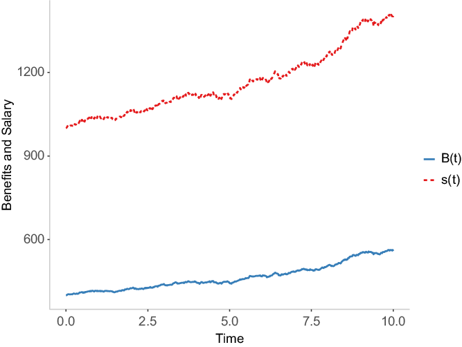
• the benefit is proportional to the salary. The percentage of salary devoted to benefit is 40%, $k=0.4$ . A path of the salary process and another of the benefit process along the planning horizon [0, 10] is plotted in Figure 1;

  Figure 1.

  Evolution of salary and benefit over time.

  

• in order to study the sensitivity with respect to the relative risk aversion parameter, we consider values $\gamma=0.5, 0.75, 1, 2$ , indicating low, moderate or high-risk aversion for the manager; for the standard case, we fix $\gamma=1$ ;

• the instantaneous rate of time preference is $\rho_1=0.05$ ; in order to study the sensitivity with respect to the discount factor associated with the terminal utility function, we consider values $\rho_2=0.05,0.15,0.25$ , that include the homogeneous case and two heterogeneous cases. $\rho_2=0.05$ will be the standard case.

The manager’s aim is to maximize an isoelastic utility function of the net benefit along the time horizon [0, T], discounted at a rate of time preference $\rho_1$ and an isoelastic utility function of the terminal fund surplus relative to salary, discounted at rate $\rho_2$ , $\rho_2\geq \rho_1$ .

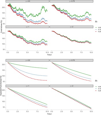
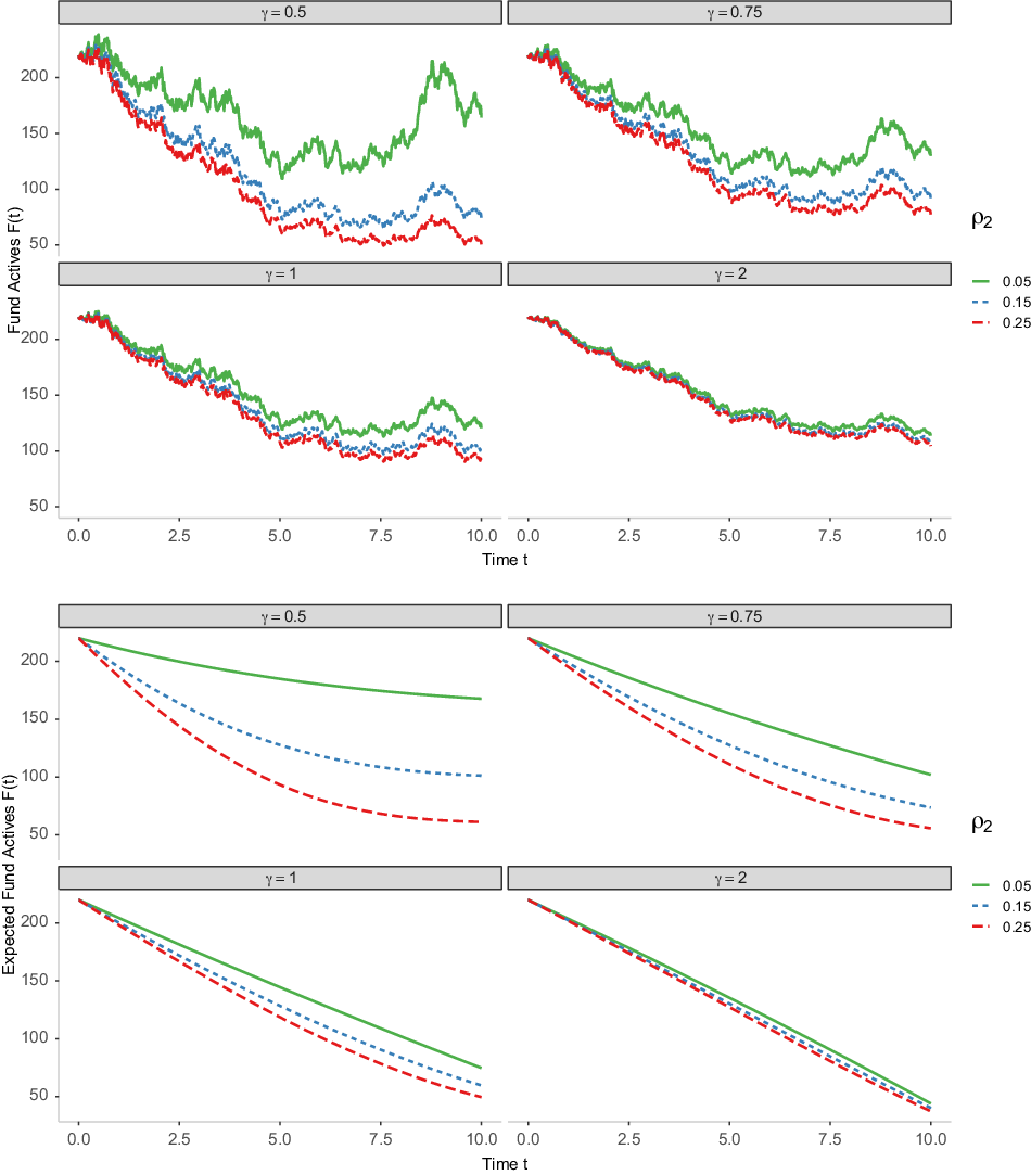
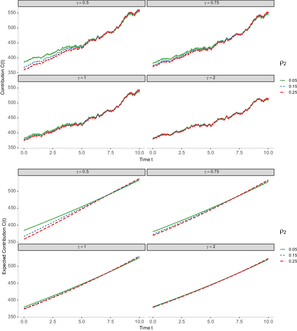
Figure 2 shows a realization of the fund $F^*$ and the expected fund $\mathbb{E} F^*=\mathbb{E}_{F_0,s_0} F^*$ for several values of the risk aversion and the rate of discount of the bequest function. As the drift of the SDE (4.8) satisfied by the fund $F^*$ is negative, the graphs show a decreasing trend. A higher risk aversion implies a higher fund. A sensitivity analysis of the fund according to the rate of discount shows that the fund decreases more slowly with a smaller rate of discount. With high-risk aversion, the dependence of the fund with respect to the rate of discount is smaller.

Figure 2.

Evolution of the fund and expected fund over time for different values of $\gamma$ and $\rho_2$ .

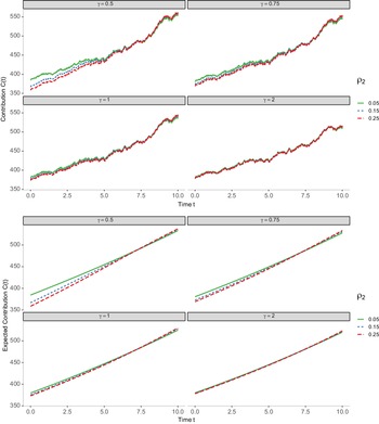
The contributions are increasing throughout almost all the planning interval. At the first instants of time, more risk aversion implies more contribution and a higher terminal rate of preference implies a lower contribution. At the last instants of time, the trend is the opposite, that is to say, a more terminal rate of preference or less risk aversion increases the contributions. Figure 3 shows a realization of the contribution $C^*$ and the expected relative contribution $\mathbb{E} C^*$ for several values of the risk aversion and the rate of discount of the bequest function.

Figure 3.

Evolution of the contribution and the expected contribution over time for different values of $\gamma$ and $\rho_2$ .

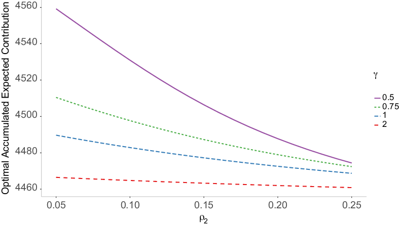
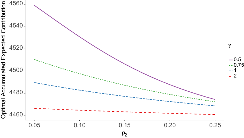
An interesting question is to analyze the accumulated expected time-consistent contribution made to the funding process by the participants through the manager, $\int_0^T \mathbb{E} C^*(t) dt$ . Figure 4 shows the total expected contribution as a function of $\rho_2$ for several values of the risk aversion. More risk aversion implies more total contribution. We observe an almost constant trend. Note that for low or moderate risk aversion, it is an decreasing function, but the gap between the lowest value of $\rho_2$ , $0.05$ , and the highest value, $0.15$ , is smaller than $0.05$ . As a conclusion, the rate of discount does not influence the total quantity contributed to the pension plan.

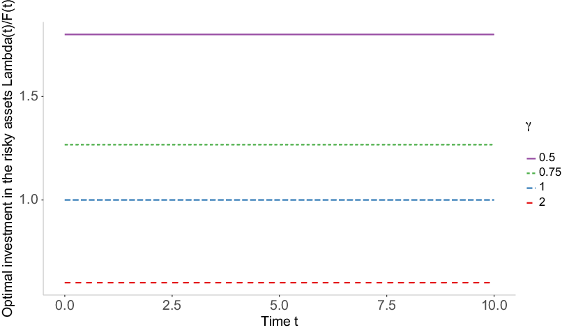
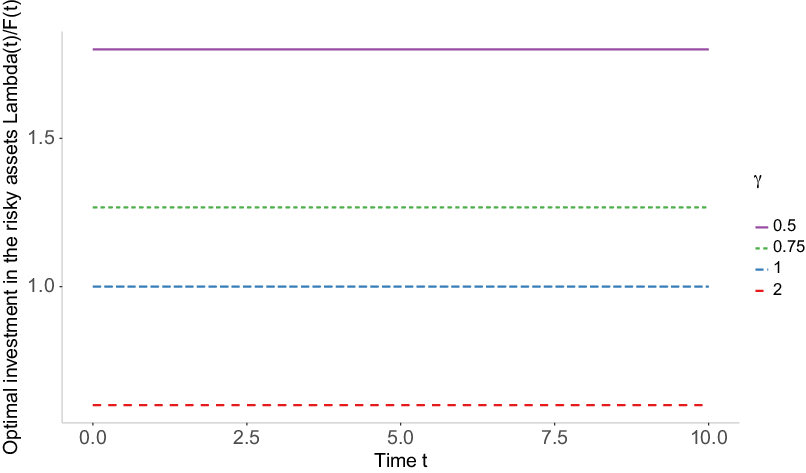
The proportion of the fund invested in the risky asset does not depend on the rate of discount and is constant along time. More risk aversion diminishes the investment. A value of $\gamma$ below $0.99$ makes it necessary to borrow to reach the time-consistent policies. However, short selling is not necessary. Figure 5 shows a realization of the time-consistent investment relative to the fund, $\lambda^*/F$ , for several values of the risk aversion.

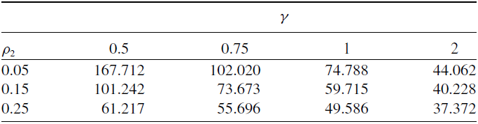
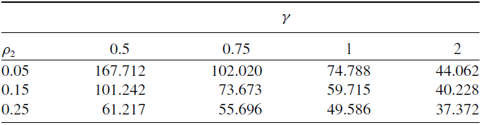
A sensitivity analysis of the expected terminal fund value, $\mathbb{E}F^*(T)$ , with respect to the risk aversion and the terminal rate of time preference can be obtained from Table 1. The terminal fund diminishes if the heterogeneity degree increases; in particular, it is higher with homogeneous discounting than with heterogenous discounting. To understand this negative effect on the terminal fund wealth, note that, from the bias generated by the heterogeneous discounting (for $\rho_2>\rho_1$ ), the decision maker initially overweights instantaneous payoffs with respect to the payoff at the end of the planning horizon, but as she moves along time this overweight decreases as the relative valuation of the final function increases. Because of this, in the case of the largest bias ( $\rho_2=0.25$ ), at the beginning of the planning horizon contributions are the lowest of the considered cases, but after some point, once the final function proportionally becomes more important, they beat contributions for the cases with a lower $\rho_2$ , as it can be observed at Figure 3. However, despite this increasing concern reflected in a higher contribution intensity, since this is the only way that the fund manager has to increase $\mathbb{E} F^*(T)$ , there is not enough remaining time to T to compensate the initially lower contributions. Consequently, $\mathbb{E} F^*(T)$ decreases when $\rho_2$ increases. A direct policy implication is that any measure oriented to reduce this bias will affect positively the value of the terminal fund. This decrease is less pronounced with high-risk aversion than with moderate or low-risk aversion. In particular, the expected terminal fund diminishes $63.5$ % in the heterogeneous case, $\rho_2=0.25$ , respect to the homogeneous case $\rho_2=0.05$ when the risk aversion is $\gamma=0.5$ ; however, the decrease is just $15.2$ % with moderate risk aversion. The terminal fund is lower when the risk aversion increases.

Table 1.

Expected terminal fund for different values of $\gamma$ and $\rho_2$ .

Figure 4.

Evolution of the total expected rate of contribution over $\gamma$ .

Figure 5.

Evolution of the proportion invested in the risky asset over time for different values of $\gamma$ .

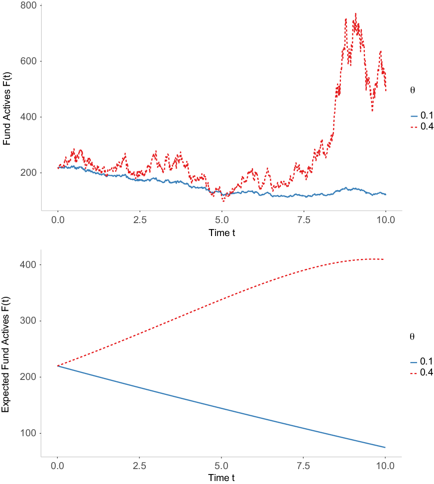
Previous analysis has been realized under a bear economic regime. An interesting question is to compare the fund evolution and the time-consistent strategies with a bull financial market. Specifically, we also now consider $\mu=0.05$ , $r=0.03$ and $\sigma=0.05$ ( $\theta=0.4$ ), for the bull regime. We keep the baseline data for the bear regime. Figure 6 shows a realization of the fund $F^*$ and the expected fund $\mathbb{E} F^*$ for the two economic regimes with moderate risk aversion ( $\gamma=1$ ). The graphs indicate a more decreasing trend with bear market than with bull market. In fact the fund is increasing in this concrete bull market. The fund diminishes from $F_0=220$ to $\mathbb{E} F(T)=74.788$ (66%) in the bear case and increases from $F_0=220$ to $\mathbb{E} F(T)=409.385$ (86%) in the bull case. We observe similar results with other values of the risk aversion parameter $\gamma$ and the market price of risk $\theta$ .

Figure 6.

Evolution of the fund and the expected fund over time for two financial markets.

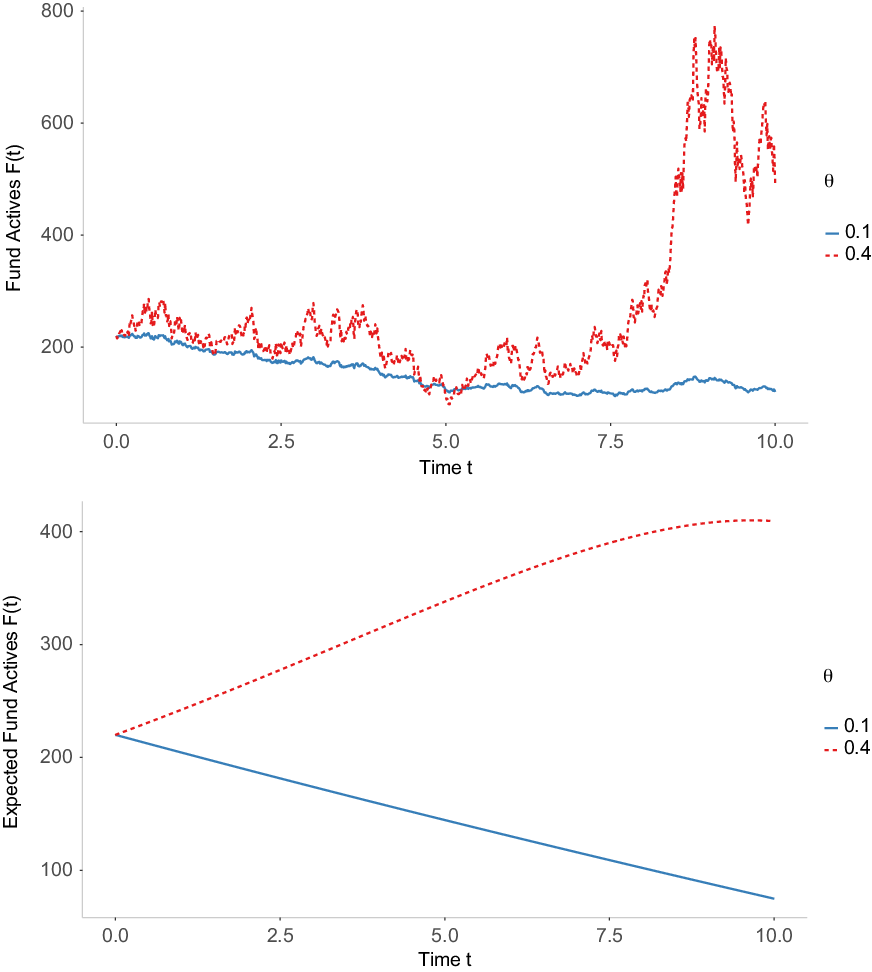
We also find a higher risky investments and contribution with the bull regime. We have also considered cases with $\rho_2<\rho_1$ . In particular, for an example of this scenario $\rho_1=0.1, \rho_2=0.05$ , the final fund value increases 22.2%. In absolute terms, 161.604 in the new scenario, versus 132.204 in the old scenario.