Nomenclature
-
 $a$
-
detective factor
-
$b$
-
updating factor
-
$Np$
-
UAV launch platform
-
$Nt$
-
number of targets
-
$Nu$
-
number of UAVs
-
${P_{loc}}$
-
location of the UAV launch platform
-
${T_{pos}}$
-
location of the target
-
${T_{ran}}$
-
target range
-
${T_{ris}}$
-
target threat coefficient
-
$TCT$
-
completion time for reconnaissance missions by UAV swarm
-
${U_{pos}}$
-
initial position of the UAV
-
${U_{ran}}$
-
maximum range of the UAV
-
${U_{spe}}$
-
cruise speed of the UAV
-
$UAF$
-
average flight time for the UAV swarm to execute reconnaissance mission
-
$UAT$
-
average threat value for the UAV swarm to execute reconnaissance mission
- UAV
-
unmanned aerial vehicle
-
$UA{V_i}$
-
UAV number
-
$UC{T_{\left( {i,k} \right)}}$
-
distance required for the i-th UAV to complete the k-th task point
-
$UT{P_{\left( {i,k} \right)}}$
-
distance from the i-th UAV to the k-th task point
-
$ris{k_{\left( {i,k} \right)}}$
-
threat value faced by the i-th UAV in completing the k-th task
-
$tc{t_i}$
-
completion time for reconnaissance missions by a single UAV
-
$ua\,{f_i}$
-
average flight time for the i-th UAV to execute reconnaissance mission


Greek symbol
-
$\alpha $
-
weight value of the complete time for reconnaissance missions by UAV swarm
-
$\beta $
-
weight value of the average flight time for the UAV swarm to execute reconnaissance mission
-
$\gamma $
-
weight value of the average threat value for the UAV swarm to execute reconnaissance mission


1.0 Introduction
In recent years, with advancements in radar detection technology, electronic jamming techniques and cooperative guidance technology [Reference Liu1], manned aircraft face increasingly complex and varied environments, posing significant challenges to their safety. UAVs have gained widespread application due to their rapid and convenient deployment, high mobility, low cost, strong self-organisation capabilities and flexible scalability [Reference Poudel and Moh2, Reference Derrouaoui, Bouzid, Belmouhoub, Guiatni and Siguerdidjane3]. Among their various applications, reconnaissance missions are one of the most typical uses for UAVs [Reference Tang, Duan and Lao4]. In practical reconnaissance tasks, UAV operational areas are often extensive, and the environments are complex. Due to the performance limitations of individual UAVs, heterogeneous UAV swarms are commonly utilised to collaboratively complete reconnaissance missions [Reference Zhang, Wen and Xiong5, Reference Peng, Wu and Xue6]. Therefore, both domestically and internationally, a series of studies have been conducted on effectively allocating tasks to harness the potential of UAV swarms fully [Reference Liu, Lin, Huang and Yan7].
Currently, solutions to the multi-UAV task allocation problem are divided into centralised and distributed methods [Reference Jia and Wang8]. Although distributed methods offer advantages such as strong robustness and flexible scalability, their inability to make globally optimal decisions based on the overall situation due to the complexity of real-world environments limits their practical application, leading to a predominant reliance on centralised methods. Among centralised algorithms, heuristic algorithms are commonly employed [Reference Yu, Gao, Wang, Wang, Ding, Lu and Zhang9].
Heuristic algorithms are widely applied in various aspects of UAVs, including task allocation [Reference Tang, Duan and Lao4], path planning [Reference Yahia and Mohammed10], scheduling [Reference Khochare, Sorbelli, Simmhan and Das11], cooperative control [Reference Basil, Sabbar, Marhoon, Mohammed and Ma’arif12], and parameter optimisation [Reference Derrouaoui, Bouzid, Doula, Boufroua, Belmouhoub, Guiatni and Hamissi13]. In the field of UAV task allocation, particle swarm optimisation (PSO) has become the mainstream algorithm due to its simple structure, minimal parameter requirements and fast computation speed. However, PSO is prone to premature convergence and struggles to solve high-dimensional complex problems, which hinders its further application. In recent years, researchers have continuously explored new approaches to address the multi-UAV task allocation problem. Reference [Reference Wang, Wang, Wei, Liu and Zhang14] improved population diversity and maintained the global optimality of the population by introducing a double crossover operator. However, this algorithm is primarily applied to large-scale task allocation problems with low convergence rates. Reference [Reference Yan, Chu, Hu and Zhu15] proposed a multi-type genetic algorithm, which significantly improved the task allocation performance through a chromosome unlocking method based on target execution sequence to handle deadlock conditions. However, the convergence rate still needs improvement. Reference [Reference Gao, Wu and Ai16] proposed a grouped ant colony algorithm. By decomposing the pheromone into sequence pheromone and membership pheromone, the arrangement and grouping characteristics of the model were effectively corresponded. Additionally, the introduction of a negative feedback mechanism accelerated the convergence speed during actual problem-solving. However, the practical results obtained from this algorithm result in a large spatial span for UAV task execution, and the algorithm incurs a high initialisation cost. Given the drawbacks of the aforementioned improved heuristic, recent years have seen scholars increasingly applying the wolf pack algorithm to the field of multi-UAV task allocation.
The wolf pack algorithm is a relatively new heuristic optimisation method that primarily solves the optimal solution by optimal solution by simulating the hunting behaviour and social division of labor of wolves. In practical applications, the wolf pack algorithm demonstrates better global search capabilities, effectively balancing local and global searches, and shows superior performance when dealing with high-dimensional complex problems [Reference Xu, Li, Zhou, Mao and Huang17]. In Ref. [Reference Wang, Ban, Ji, Guan, Liu and Qian18], an adaptive shrinking grid chaotic wolf pack optimisation algorithm (ASGS-SWOA) is proposed. This algorithm enhances the search ability of the wolf pack through an adaptive shrinking grid strategy, while employing the intermediate raid method (OMR) to accelerate the algorithm’s convergence speed. In Ref. [Reference Chen, Cheng, Liu, Cheng and Mao19], the OGL-WPA algorithm is introduced. This algorithm initialises the wolf pack using an adversarial learning strategy to improve population diversity and expand the global search space. Meanwhile, during the algorithm’s iterations, the genetic algorithm is used to select the leader wolf, helping the algorithm escape local optima to some extent. Reference [Reference Zhu, Wu, Li and Hu20] proposes a chaotic disturbance wolf pack algorithm, which improves the quality of initial solutions through the chaos and introduces disturbance factors to enhance the search ability of the wolf pack, thus avoiding local optima. Reference [Reference Wang, Zhu, Zhou and Sun21] introduces a three-leader wolf mechanism, where one leader wolf is randomly selected to influence the position update. A logistic function is also incorporated into the convergence factor to optimise the algorithm’s solution accuracy.
Although scholars have continuously attempted to improve the initial solution quality, enhance solution accuracy, and maintain population diversity in the wolf pack algorithm, most of the improvements are still at the stage of single-population and single-optimisation mode. The multi-UAV task allocation problem is a high-dimensional discrete problem. The single-population wolf pack algorithm results in all individuals sharing the same search space, which often leads to local optimal in multimodal problems. Additionally, the single-population algorithm is heavily dependent on local optima, and when applied to multi-UAV task allocation, it tends to be guided by a local optimum, thus deviating from the optimal optimisation direction.
Based on the limitations of single-population algorithm, multi-population algorithms have received increased attention from researchers due to their superior ability to explore solution spaces and maintain population diversity [Reference Ma, Shen, Yu, Yang, Fei and Zhou22]. Reference [Reference Vafashoar and Meybodi23] proposes a multi-population method with fixed subpopulation size, innovatively employing a reverse convergence approach to randomise already converged sub-populations, thereby avoiding the entrapment of populations in local optima. Reference [Reference Raghul and Jeyakumar24] introduces an algorithm that forms a fixed number of sub-populations based on the division of the search area. This algorithm helps maintain population diversity by employing mechanisms based on success rates and population aging. Reference [Reference Qin, Huang and Luo25] presents a multi-population algorithm with an adaptive number of sub-populations; however, in this algorithm, the number of individuals in each sub-population is fixed. Due to its adaptability, the overall population size may vary. Additionally, a mechanism for removing the redundant sub-population sub-populations is introduced to prevent the waste of computational resources, enhancing the algorithm’s performance.
Multi-population algorithms can generally be categorised into those with fixed subpopulation sizes and those with dynamic subpopulation sizes. Algorithms with fixed subpopulation sizes are effective in expanding the search space, but they sacrifice the convergence speed to some extent. Moreover, when dealing with complex problems, these algorithms lack efficiency and flexibility. On the other hand, algorithms with dynamic subpopulation sizes achieve more efficient searching and faster convergence by flexibly adjusting the number and size of populations. However, existing algorithms often handle redundant subpopulations by deletion or reconstruction operations. While these operations help avoid the waste of computational resources, they also introduce additional computational overhead, especially when dealing with complex, large-scale problems. Furthermore, excessive deletion or reconstruction operations may negatively affect the algorithm’s stability and global search capability.
Based on the issues identified in existing multi-population algorithms mentioned above, and building upon our previous work [Reference Zhang, Lv, Ma and Cui26] as well as being inspired by Refs [Reference Qin, Li, Zhang and Fu27, Reference Yang, Zhou, Li, Guan and Yan28], this paper innovatively proposes a two-stage dynamic subpopulation size wolf pack algorithm. The main contributions are as follows and to distinguish the differences between our current work and previous work, we have listed a brief summary of the distinctions in Table 1.
-
(1) Two-stage approach. In the field of multi-UAV task allocation, and in contrast to the traditional single-solution framework. This paper innovatively proposes a two-stage solving approach. In the early stage, the algorithm focuses on minimising the UAV resource usage cost, while in the later stage, it emphasises fine-tuning the task execution plans for the existing UAV resources. By decomposing the complex problem into two subproblems, the difficulty of problem-solving is effectively reduced, the algorithm’s solving speed is accelerated, and the scalability of the algorithm is enhanced.
-
(2) Dynamic multi-population mechanism. Unlike traditional dynamic multi-population mechanisms, this paper innovatively introduces a dynamic multi-population mechanism based on the average contribution of subpopulations. Specifically, after each iteration, the average contribution of each subpopulation to the optimal solution is calculated, enabling the dynamic allocation of computational resources within each subpopulation. In contrast to recent approaches to redundant subpopulation handling, this paper proposes innovative mechanisms for population protection, migration and communication. These mechanisms facilitate high-quality optimisation through mutual assistance among populations rather than relying on traditional operations such as deletion or reconstruction of subpopulations.
The differences between this work and previous work

The remainder of this paper is organised as follows: Section 2.0 presents the multi-UAV task allocation model. Section 3.0 introduces the proposed 2SMPWPA algorithm. Section 4.0 analyses the configuration of the algorithm parameters and validates the performance of the proposed algorithm through comparative experiments with similar algorithms, followed by an analysis of the experimental results. Section 5.0 summarises the entire paper and offers an outlook on future work.
2.0 Task modeling
In practical application scenarios, our team can obtain prior information, such as the locations of reconnaissance targets and the extent of target areas through satellites and other means. Subsequently, we deploy a swarm of UAVs from a launching platform to conduct close reconnaissance on multiple targets. The reconnaissance task is divided into three parts: the UAVs depart from the launching platform, the UAVs patrol the target area, and the UAVs return to the launching platform. The reconnaissance task is considered complete once all UAVs have fulfilled their assigned missions.
In the paper, the model specifies four types of UAVs and four launching platforms (each platform comprises different types of UAVs). The number of UAVs can be adjusted based on practical considerations. The location of the launching platforms, as well as the number, locations and sizes of the reconnaissance targets, are randomly generated within defined constraints.
2.1 The optimisation objectives
To align the model more closely with the practical scenarios, this paper considers three optimisation criteria: the completion time of the UAV swarm reconnaissance mission, the average flight time of the UAV swarm and the average threat coefficient faced by the swarm.
2.1.1 Completion time of the reconnaissance mission
The task completion time is one of the most critical metrics for evaluating the effectiveness of task allocation. The shorter the completion time for the UAV swarms, the higher the efficiency of mission execution. The completion time for reconnaissance tasks consists of the time the UAVs take to reach the target point and the time required to complete the target reconnaissance. Completing a reconnaissance mission refers to successfully executing the reconnaissance tasks by all dispatched UAVs. The specific calculations are presented in Equation (1):
 \begin{align}TCT = \mathop {{\rm{max}}}\limits_{x \in \left( {1,Nu} \right)} {\rm{\;\;}}tc{t_i}\end{align}
Where tct
 ${\;_i}$
represents the time the ith UAV took to complete the reconnaissance task. The task completion time for a single UAV is expressed by Equation (2):
 \begin{align} tc{t_i} = {{\mathop \sum \nolimits_{i = 1}^{Nu} \mathop \sum \nolimits_{k = 1}^n UT{P_{\left( {i,k} \right)}} + UC{T_{\left( {i,k} \right)}}} \over {{U_{spe}}}}\end{align}
In Equation (2), UTP
 ${\;_{\left( {i,k} \right)}}$
denotes the distance between the current position of the ith UAV and the kth task point. UCT
 ${\;_k}$
represents the distance that the UAV needs to fly to complete the kth task, while
 ${U_{spe}}$
indicates the flight speed of the UAV.
2.1.2 The average flight time of the UAV swarm
The average flight time of the UAV swarm provides an intuitive measure of the load balancing among the UAVs during the mission. A longer average flight time indicates an unreasonable task distribution, resulting in some UAVs being overloaded; conversely, a shorter average flight time suggests a more balanced allocation of tasks. The flight time of the UAV swarm consists of three components: the time taken for the UAV to reach the target point, the time spent executing the reconnaissance task, and the time taken for the UAV to return to the launch platform, as illustrated in Equation (3):
 \begin{align}ua\,{f_i} = \frac{{tc{t_i} + PTP}}{{{U_{spe}}}}\end{align}
Equation (3) represents the calculation of the flight time for a single UAV while executing a reconnaissance task. PTP denotes the distance the UAV travels to return to the launch platform after completing the last task. The average flight time of the UAVs is calculated by dividing the sum of the flight times of all UAVs by the total number of UAVs, as illustrated in Equation (4):
 \begin{align}UAF = {{\mathop \sum \nolimits_{k = 1}^{Nu} ua\,{f_k}} \over {Nu}}\end{align}
2.1.3 The average threat value of the UAV swarm
The average threat value of the UAV swarm measures the mean level of threats faced by the swarm during the mission execution. A higher average threat value indicates that the UAV swarm is exposed to greater risks while performing tasks, which decreases the likelihood of mission success and suggests a more unreasonable task distribution. This paper associates the threat value of a target with its range, meaning that a larger target range results in longer exposure times for the UAVs during the reconnaissance tasks, thereby increasing the threat value. The calculation of the average threat value of the UAV swarm is shown in Equation (5):
 \begin{align}UAT = {{\mathop \sum \nolimits_{i = 1}^{Nu} \mathop \sum \nolimits_{k = 1}^{Nt} ris{k_{\left( {i,k} \right)}}} \over {Nu}}\end{align}
2.2 Objective function
The objective function is constructed from optimised objects and assigned corresponding weights, as shown in Equation (6):
 \begin{align} fitness = \alpha \times TCT + \beta \times UAF + \gamma \times UAT\end{align}
In the scenarios of multi-UAVs executing reconnaissance missions, the UAVs face threats from uncertainties in the target area. Therefore, this paper considers the average threat of the UAV swarm as the most important evaluation metric, ensuring that the UAVs can safely complete their assigned tasks. Additionally, the completion time of reconnaissance missions and the average flight time of the UAV swarm are regarded as secondary metrics that help to ensure that the UAVs can complete their assigned tasks at the minimum cost. In summary, this paper sets
 $\alpha = \beta = 0.3,\gamma = 0.4$
. To ensure the model’s generality, the weights of the optimisation objectives can be adjusted according to the actual needs of the scenario, subject to the constraints [Reference Xu, Li, Zhou, Mao and Huang17, Reference Zhu, Li, Teng and Yonglu29].
2.3 Constraints condition
To construct a general model, the only constraint for the task allocation scheme in this model is that it must not exceed the maximum flight range of the UAVs. When the task allocation scheme does not satisfy this constraint, the fitness value of the scheme is set to ‘inf’. Additional constraints can be incorporated based on the requirements of practical applications. The addition of constraints will affect the results of the task allocation but will not fundamentally impact the solving performance of the algorithm.
3.0 Proposed 2smpwpa algorithm
This paper proposes a 2SMPWPA to solve the task allocation model. The essence of the 2SMPWPA algorithm is to divide the solution of the multi-UAV task allocation problem into two stages: the early stage focuses on determining the optimal UAV resource allocation, while the latter stage emphasises optimising the task allocation scheme for the existing UAV resources.
Unlike traditional multi-population algorithms with fixed sub-population size, the 2SMPWPA algorithm categorises the population into one leader group and two normal groups. During the iterations, dynamic population sizing is achieved by calculating the average contribution of each sub-population to the optimal solution. However, this may lead to a big-eats-small phenomenon within the sub-populations. The algorithm introduces population protection and migration mechanisms to address this issue.
Finally, to prevent sub-populations from becoming trapped in local optima, this algorithm introduces a population communication mechanism, which endows the algorithm to escape local optima through interactions among sub-populations. The pseudocode is presented in Algorithm 1, where the iterative computations encompass mechanisms such as wandering, calling, sieging and individual reconstruction.
The iterative computation of the algorithm consists of wandering behaviour, calling behaviour, sieging behaviour, and individual reconstruction mechanism, as shown in Fig. 1. The algorithm proposed in this paper shares the same interaction mechanisms of basic behaviours as other wolf pack algorithms. Specifically, wandering behaviour explores potential optimal solution spaces through random search. Calling behaviour enables rapid convergence of the population by facilitating learning from the head wolf. Sieging behaviour further refines the search within regions containing excellent solutions. The individual reconstruction mechanism avoids local optima by reconstructing poorly performing individuals, thus enhancing the global search ability of the algorithm. The interaction patterns of these four mechanisms remain consistent in both the early and late stages. However, there are differences in the specific implementation of the algorithm, as detailed in Sections 3.6–3.9 and our previous work [Reference Zhang, Lv, Ma and Cui26].
Algorithm flowchart.

Compared to similar algorithms, the two-stage solution approach proposed in this paper, when solving the multi-UAV task allocation problem, divides the complex problem into two simpler sub-problems, thus reducing the difficulty of solving complex issues. Additionally, by focusing on solving one key problem at each stage, this approach also helps improve the algorithm’s solution accuracy. Moreover, the two-stage solution approach enhances the scalability of the algorithm, making it adaptable to various scenarios. For instance, in extreme scenarios where UAV resources are prioritised, more computational resources can be allocated to the early stage; in scenarios with higher demands for the quality of UAV task completion, more computational resources can be allocated to the later stage.
The multi-population model proposed in this paper calculates the average contribution of each sub-population to the overall optimal solution, allowing computational resources to be more accurately allocated to the sub-populations that perform well. Moreover, when handing poorly performing sub-populations, this algorithm differs from traditional methods such as deletion and reconstruction, instead employing population protection and migration. By introducing superior individuals from high-performing sub-populations, this approach helps poorly performing sub-populations escape the current local solution space in a smoother process. The final population communication mechanism also facilitates information sharing between sub-populations, which not only helps to expand the search for the solution space by high-performing populations but also assists poorly performing sub-populations in escaping local optima.
2SMPWPA

3.1 Initialisation phase
Individual initialisation refers to generating a dedicated Tn and Un list for each individual in the population. The Tn list is a task identification list that contains the identifiers of all tasks to be executed. During initialisation, the identifiers of all pending tasks are randomly shuffled and placed in the Tn list, ensuring that each task identifier appears only once, indicating that each task will be executed only once. The Un list is UAV identifiers that contain the identifiers of all UAVs. During initialisation, UAV identifiers are randomly generated and added to the Un list, where a single UAV identifier may appear multiple times, signifying that the UAV can perform multiple tasks. The execution order of the tasks is determined by the sequence in which the task identifiers appear in the Tn list. The corresponding columns in the Tn and Un lists can be viewed as a whole, representing the assignment of a specific task to a particular UAV for completion.
Population initialisation refers to the process by which the algorithm divides the population into two main categories: the normal group and the leader group. The normal group consists of two sub-populations; assuming a total population size of N, the size of each sub-population is
 $\frac{2}{N}$
. The leader group is unique and comprises individuals ranked in the top 20% of fitness values from the sub-populations, resulting in a leader group size of
 $0.2 \times N$
.
3.2 Dynamic population mechanism
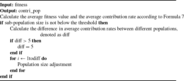
The initial intention behind the design of the dynamic population mechanism is to allocate computational resources preferentially to the better-performing sub-population, thereby enhancing the overall convergence speed of the algorithm. The dynamic adjustment of sub-population sizes is achieved by calculating the average contribution of each sub-population to the optimal solution, as illustrated in Equation (7):
 \begin{align} contri\_pop = \frac{{int\left( {avg\,fi{t_i} - best\,fit} \right)}}{{len\left( {po{p_i}} \right)}}\end{align}
In the equation, avgfit
 ${\;_i}$
represents the average of the fitness values of all individuals in sub-population i, while bestfit denotes the best fitness value obtained in the current iteration. The function len(
 $po{p_i}$
) indicates the size of sub-population i. The function int() is used to round the nearest integer. The difference in average contribution among the sub-populations determines the adjustment in population size. The pseudocode is presented in Algorithm 2.
Dynamic Population Mechanism

3.3 Population protection mechanism
The population protection mechanism is designed to prevent the overconsumption of inferior subpopulations by superior subpopulations. This mechanism first restricts the adjustment of population sizes in each iteration, limiting changes to a maximum of five individuals. This restriction aims to prevent excessive disparities among sub-populations during the initialisation phase, which could result in a well-initialised sub-population rapidly absorbing a significant portion of another sub-population’s size. Since the initialisation result does not necessarily represent the optimal solution direction, this could lead to suboptimal performance of these populations in subsequent iterations. In order to ensure that poorly performing subpopulations are not eliminated, the population protection mechanism sets a lower limit for the size of each subpopulation. If the size of a subpopulation falls below this limit, it will trigger the population migration mechanism, which will be described in the following section.
3.4 Population migration mechanism
The population migration mechanism is designed to ensure that sub-populations with poorer performance retain a certain level of optimisation capability. When the size of a sub-population falls below the established lower limit, this sub-population will absorb individuals from the higher-performing sub-population. The absorbed individuals will guide the updating of local individuals, thereby enhancing the solution performance of the poorer sub-population.
The population migration mechanism, by transferring high-performing individuals from well-performing populations to the poorly performing population, helps the latter escape local optima, thereby accelerating the algorithm’s convergence to the global optimum. Additionally, the migration mechanism increases information sharing between populations, enhancing population diversity. The introduction of high-quality individuals can prevent premature convergence to a local optimum, thereby improving convergence accuracy. This is particularly important when solving high-dimensional complex problems. The pseudocode for this mechanism can be found in Algorithm 3.
population Migration Mechanism

3.5 Population communication mechanism
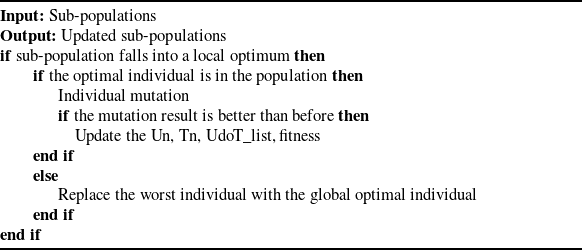
Under the multi-population mechanism, the small number of individuals in each sub-population results in limited coverage of the solution space, which can easily lead to convergence to local optima. To address this issue, the algorithm introduces a population communication mechanism. When a sub-population undergoes a certain number of iterative computations without any change in the optimal solution, it is deemed to have fallen into a local optimum, thereby triggering the population communication mechanism.
The population communication mechanism can trigger in two scenarios: when the sub-population containing the optimal solution becomes trapped in a local optimum, or another sub-population falls into local optima. When an ordinary sub-population is trapped in a local optimum, the worst-performing individual in that sub-population is replaced with the global best individual to assist the sub-population in escaping the local optimum. Conversely, mutation operations are performed on the global best individual when the sub-population containing the optimal solution becomes trapped in a local optimum. These mutation operations target each column in the Un list of the global best individual, and the mutation range is limited to those UAVs that have been assigned tasks (i.e., the solution obtained in the early stage of the algorithm). After each mutation, the fitness value is compared to that before mutation: if it improves, the change is retained; otherwise, no changes are made. The pseudocode for this mechanism can be found in Algorithm 4.
Population Communication Mechanism

3.6 Wandering behaviour
In the context of multi-UAV task allocation, the wandering behaviour can be utilised to optimise the execution order of tasks. The number of detective wolves is randomly generated within the range of
 $\left( {\frac{N}{{a + 1}},\frac{N}{a}} \right)$
, where a is the detective factor, as indicated in Equation (8):
 \begin{align}D\_num = Random.randomInt\left( {\frac{N}{{a + 1}},\frac{N}{a}} \right)\end{align}
3.6.1 Wandering behaviour of the normal group
The primary objective of the early stage is to identify the optimal allocation of UAV resources. Therefore, this stage allocates limited computational resources to the wandering behaviour, specifically by employing a fixed and relatively low number of wandering times, denoted as Tmax, to optimise the sequence of tasks executed by the UAVs.
The primary objective of the later stage is to optimise the task execution scheme for UAV resources, which includes the order in which the UAVs execute tasks. Unlike the early stage, this stage employs an adaptive wandering time strategy. The adaptive wandering times involve calculating the number of possible permutations of task execution sequences. The computed result is then used to determine the number of wandering times for that particular detective wolf concerning the specific UAV. When dealing with large-scale problems, a single UAV may need to execute 10 or more tasks. In such cases, the number of adaptive wandering times can become excessively large, presenting challenges to the algorithm’s runtime. Therefore, a maximum truncation can be applied to the adaptive wandering times.
3.6.2 Wandering behaviour of the leader group
The wandering behaviour of the leader group is in contrast to that of the normal group at different stages. Specifically, the leader group employs an adaptive wandering time in the early stage and a fixed wandering time in the later stage. In the early calculations of the leader group, in order to reduce the influence of the suboptimal task execution order on the solution of UAV resource allocation, the leader group needs to invest a large amount of computing resources to obtain the best task execution order. In the later stage of the algorithm, the normal group has already invested considerable computational resources in determining the UAV task execution sequence. As a result, in the leader group, there is no need for redundant calculations; instead, it is sufficient to perform a fixed and limited number of wandering time to conduct tasks similar to ‘verification’.
3.7 Calling behaviour
The calling behaviour is a critical step in achieving convergence within the algorithm. Essentially, it involves the fierce wolves in the pack learning from the task allocation strategy of the head wolf, thereby facilitating the individual wolves’ approach to the optimal solution. Both the leader group and the normal group implement different strategies for calling behaviour at various stages, which will be detailed in the following sections.
3.7.1 Calling behaviour of the normal group
The normal group’s early and late calling behaviours exhibit similarities, primarily differing in their convergence speeds. In the early stage, each wolf generates a random integer within the range of
 $\left[ {0,Nt - 1} \right]$
. This integer indicates the number of columns from the head wolf that need to be learned during this round of iterative calculations. Subsequently, another random integer is generated within the same range
 $\left[ {0,Nt - 1} \right]$
to specify the particular column from which the head wolf’s information will be learned.
In the later stage, to prevent premature convergence, it becomes necessary to regulate the convergence speed of the fierce wolves. Consequently, in each round of iterative calculations, the number of columns that the fierce wolves learn from the head wolf is limited by generating random integers within the range of
 $\left[ {0,0.2 \times Nt} \right]$
. Similarly, a random integer is generated within the range of
 $\left[ {0,Nt - 1} \right]$
to denote the specific column learned from the head wolf.
3.7.2 Calling behaviour of the leader group
The calling behaviour of the leader group essentially represents a process of mutual learning from the well-performing individuals within the normal group. In the early stage of the leader group, the strategy for calling behaviour is the same as that employed in the later stage of the normal group. This approach is designed to prevent excessive convergence within the leader group, which could result in different sub-populations converging to the same local optimum. In the later stage, the leader group distinguishes the early stage by combining the calling behaviour with the sieging behaviour. The specific details of the combined approach can be found in Section 3.8.2.
3.8 Sieging behaviour
In the context of multi-UAV task allocation, sieging behaviour is primarily employed to balance exploration and exploitation. Given that the algorithm decomposes the solution process into two stages, each with different focal points. Sieging behaviour adopts varying strategies across different stages and populations.
3.8.1 Sieging behaviour of the normal group
In the normal group, sieging behaviour employs a ‘probability threshold’ strategy for problem-solving. The probability threshold P is derived by calculating the fitness difference between the head and individual wolf. This threshold is then compared with a random number; when P exceeds the random number, the sieging behaviour emphasises exploration. Conversely, when P is less than the random number, the algorithm focuses on exploiting the task allocation experience of the head wolf.
In the early stage of the algorithm, to explore a broader range of combinations for UAV utilisation, the exploration scope encompasses all available UAVs. Simultaneously, to prevent premature convergence, the exploitation does not solely rely on the task allocation experience of the head wolf; instead, any individual wolf that performs better than the current individual can serve as a valid example for exploitation. In the later stage, after multiple iterations, it is assumed that the optimal UAV resource allocation has been identified. Consequently, in this stage, the exploration scope is restricted to the UAVs that have already been assigned tasks, and exploitation is based exclusively on the head wolf as the learning example.
3.8.2 Sieging behaviour of the leader group
In the early stage of the leader group, to avoid excessive similarity among individuals and to balance the needs for exploration and exploitation, the sieging behaviour is implemented using a random strategy. Specifically, a random number is generated within the range of
 $\left[ {1,{\rm{\;\;}}Nt - 1} \right]$
, indicating the number of columns to be altered for the individual in this iteration. Then, another random number
 $r$
is generated within the range of
 $\left[ {0,1} \right]$
and compared to 0.5. If
 $r \lt 0.5$
, the sieging behaviour randomly mutates a task allocation result. Conversely, if
 $r \gt 0.5$
, the sieging behaviour learns from the task allocation schemes of individuals that outperform the current individual wolf.
In the later stage, to accelerate convergence, when the random number exceeds 0.5, only the head wolf’s task allocation scheme for a specific task is learned. When the random number is less than 0.5, in order to prevent excessive similarity among individuals, the number of altered columns must be restricted. Specifically, the number of columns to be changed is determined within the range of
 $\left[ {1,Nt \times 0.2} \right]$
, after which random mutation is performed as in the early stage of the leader group.
3.9 Individual reconstruction
Individual reconstruction refers to improving the algorithm’s capability by reconstructing poorly performing individuals to positions near high-quality solutions. Except for the leader group’s later stage, individual reconstruction is performed using a roulette wheel mechanism across all other populations and phases. Specifically, during each round of individual reconstruction, only the task allocation schemes of elite individuals (those in the 20% based on fitness ranking) within each population are considered. Based on the statistical results, a ‘roulette’ is generated, where the proportion of each task allocation scheme among the statistical samples is calculated to assign corresponding weight values (with the total weight summing to 1). Subsequently, a random number is generated within the range
 $\left[ {0,1} \right]$
, and the task allocation scheme for the newly generated individuals is determined based on the interval in which the random number falls on the roulette. This process is illustrated in Fig. 2.
Roulette wheel diagram.

The left side of Fig. 2 displays the statistical results of task allocation schemes for task i among elite individuals in the wolf pack, where the number within the circle represents the UAV identifiers. The roulette on the right is constructed based on the statistical results presented on the left. For instance, six elite individuals’ task allocation schemes have been recorded on the left, with two elite individuals assigning task i to the fourth UAV. Consequently, during individual reconstruction, there is a 33% probability of allocation of task i to the fourth UAV.
3.10 Analysis of algorithm time complexity
This paper primarily proposes a two-stage, multi-population mechanism and a roulette-wheel-based wolf population individual reconstruction mechanism. The remaining sections of the chapter will focus on analysing the time complexity of these three components, with the aim of verifying the algorithm’s performance in solving real-world problems.
The two-stage model is essentially a decision statement, so its time complexity is O(1), as can be seen in Line 9 of Algorithm 1. In the dynamic population mechanism, the time complexity is primarily determined by the population size adjustment. However, due to the constraints imposed by the population protection mechanism, the maximum number of individuals that can be added or removed from a subpopulation is limited to 5. Therefore, the time complexity is O(N), as detailed in Algorithm 2. The population protection mechanism is essentially composed of two conditional statements: one checks whether the number of individuals moved in each iteration exceeds the threshold, and the other verifies whether the size of a subpopulation falls below the minimum value. Therefore, the time complexity of this part is O(1). The population migration mechanism essentially transfers high-performing individuals from the superior sub-population to the sub-population with poorer performance, assisting the latter in quickly escaping suboptimal solution space. The time complexity of this mechanism is primarily influenced by the number of individuals being transferred. Therefore, the time complexity of this mechanism is O(N), as detailed in Algorithm 3. In the population communication mechanism, the most time-consuming task is determining whether the global best individual is present in the sub-population. Therefore, the time complexity of this part is O(N), as detailed in Algorithm 4. The core of the roulette-wheel-based wolf individual reconstruction mechanism is to identify the individuals to be reconstructed and task allocation scheme for selecting the superior individuals in the wolf pack. Thus, the time complexity of this part is O(
 ${N^2}$
).
This paper provides a detailed analysis of the complexity of each component of the 2SMPWPA algorithm. The analysis shows that the overall time complexity of the algorithm is primarily influenced by the individual reconstruction mechanism. However, when dealing with complex problems, traditional random individual reconstruction mechanisms do not adequately meet the solving conditions, leading to slow convergence. On the other hand, the current elite-based individual reconstruction mechanism tends to cause premature convergence, making it prone to local optima. Therefore, although the roulette-wheel-based reconstruction mechanism proposed in this paper introduces some computational overhead, it significantly improves solution accuracy when handling large-scale complex problems. In conclusion, it can be demonstrated that the time complexity overhead of the algorithm is acceptable, and the algorithm is feasible for solving real-world problems.
4.0 Comparative experiment
This section focuses on a series of ablation and comparison experiments in the context of multi-UAV collaborative reconnaissance missions. UAV reconnaissance refers to the process where UAV, equipped with visible light cameras and infrared cameras, take off from the launch platform, approach the target and conduct reconnaissance to obtain detailed data about the target. During the reconnaissance process, UAVs are required to cover the entire target area. Once all UAVs have completed their respective tasks and returned to the launch platform, the reconnaissance mission is considered complete. In the experiments of this chapter, unless otherwise specified, it is assumed that there are four UAV launch platforms, which are randomly generated within the region
 $\left[ {0,100\left] \times \right[0,100} \right]$
. Additionally, there are 10 UAVs of 4 different types and 25 reconnaissance tasks. Detailed information is provided in Table 2.
UAVs parameters

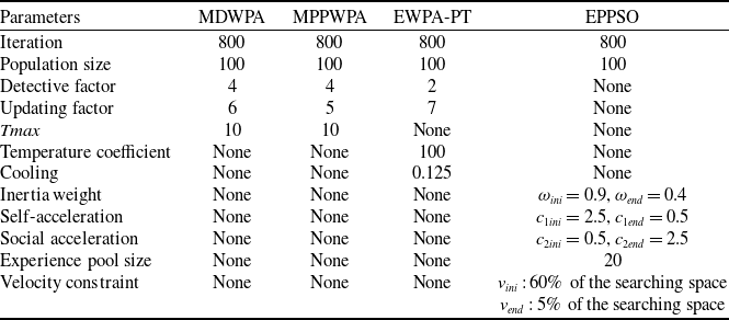
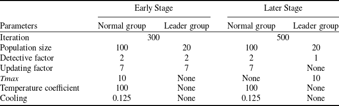
To ensure the fairness of the experiments, all experiments in this section are based on 50 repeated runs to draw conclusions. In the experiments, we select the outstanding EPPSO algorithm from the particle swarm optimisation category, as well as the high-performance multi-discrete wolf pack algorithm (MDWPA), multi-population parallel wolf pack algorithm (MPPWPA), and elite wolf pack algorithm based on probability threshold (EWPA-PT) algorithms from the pack optimisation category. The parameters for the comparative algorithms are consistent with those specified in the original literature, as detailed in Table 3. The parameter selection for our algorithm is presented in Table 4, with the rationale for the parameter choices discussed in ablation experiments in Section 4.1.
Comparison of algorithm parameter settings

2SMPWPA algorithm parameter settings

4.1 Ablation experiment
4.1.1 Ablation experiment of parameter a
Parameter a is the detective factor, which determines the number of detective wolves generated in each iteration and is an important parameter affecting the wandering behaviour. In the ablation experiment of the subsection, we set the value of parameter a to all integers from 1 to 9 and test its impact on the average value and average runtime of the algorithm at each population and stage, as illustrated in Fig. 3–6.
Parameter a in the Early-stage of the normal group.

Parameter a in the late-stage of the normal group.

Parameter a in the early-stage of the leader group.

Parameter a in the late-stage of the leader group.

From the figures, it can be observed that parameter a has a direct impact on both the fitness value and the algorithm’s runtime. In particular, as shown in Fig. 4, during the later stage of the normal group, an increase in the value of parameter a leads to a reduction in runtime, albeit at the cost of decreased solution accuracy (the reduced accuracy still surpasses that of the comparative algorithms, which will be discussed in Section 4.2). Therefore, in scenarios where strict requirements are placed on the algorithm’s runtime, it may be beneficial to adjust the value of parameter a to meet the specific needs of those scenarios.
4.1.2 Ablation experiment of parameter b
Parameter b is the update factor that determines the number of individual wolves to be reconstructed in each iteration. Different values of parameter b significantly affect the algorithm’s individual reconstruction mechanism. In the ablation experiments of this subsection, we set the value of parameter b to all integers from 1 to 9 and record its impact on the average fitness value and average runtime of the algorithm, as illustrated in Figs. 7–9.
Parameter b in the early-stage of the normal group.

Parameter b in the late-stage of the normal group.

Parameter b in the early-stage of the leader group.

Due to the absence of an individual reconstruction mechanism in the leader group during the later stage, the ablation experiments in this subsection do not include the impact of parameter b on the algorithm’s performance in this situation. From the above, it can be observed that values of parameter
 $\beta $
between 6 and 7 contribute maximally to the algorithm’s overall performance.
4.1.3 Ablation experiment on two-stage proportions
This algorithm divides the multi-UAV task allocation problem into two parts, with 800 iterations. The ablation experiments in the subsection aim to explore the impact of different proportions of iterations in the early and later stages of task resolution on the algorithm’s overall performance. By systematically adjusting the number of iterations at each stage, the optimal stage proportions can be determined, thereby enhancing the overall performance of the algorithm, as shown in Fig. 10.
Two-stage ratio ablation experiment.

The experimental results indicate that the algorithm achieves the best solution performance when the two-stage ratio is 3:7. This is primarily because the main task in the early stage is to optimise UAV resource allocation, which is relatively straightforward. Therefore, a lower proportion in the early stage can both satisfy the task-solving requirements and reserve sufficient computational resources for solving the optimal task execution order in the later stage. As the early-stage proportion increases and the later stage decreases, the algorithm’s solution accuracy gradually declines. This is mainly due to the fact that the simpler tasks in the early stage consume a large amount of computational resources, leaving the more complex tasks in the later stage insufficiently addressed. In summary, the optimal ratio for the two stages is 3:7.
4.2 Comparative experiments under different conditions
4.2.1 Comparative experiments of different target areas
The distribution of target areas significantly affects the outcomes of multi-UAV task allocation. When the target area is relatively close to the launch platform, it is advisable to deploy UAVs with shorter ranges and faster flight capabilities to conduct reconnaissance tasks. Conversely, when the target area is far from the launch platform, it may be necessary to sacrifice task completion time to ensure the mission’s feasibility. In this case, longer-range UAVs with slower flight speeds should be dispatched to accomplish the tasks. In this subsection, we comprehensively compare several recent algorithms that have shown excellent performance, including the enhanced particle swarm optimisation (EPPSO), the single-population wolf pack algorithm (MDWPA, EWPA-PT), and the multi-population wolf pack algorithm (MPPWPA). In the experiments, we fix the number of UAVs at 10 and the number of tasks at 25. Additionally, six different task distribution scenarios (
 $[ 0,100] \times [0,100] {,{\rm{\;\;}}} [50, 150] \times [50,150] {,{\rm{\;\;}}} [100,200] \times [100,200] {,{\rm{\;\;}}} [150, 250] \times [150,250] {,{\rm{\;\;}}}$
 $[200,300] \times [200,300] {,{\rm{\;\;}}} [250,350] \times [250,350].$
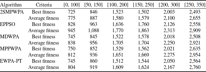
) are selected for testing. For each target distribution scenario, we repeat the experiment 50 times and calculate the average fitness value after each iteration. The detailed results are presented in Figs. 11–16 and Table 5.
Targets are distributed over [0, 100].

Targets are distributed over [50, 150].

Targets are distributed over [100, 200].

Targets are distributed over [150, 250].

Targets are distributed over [200, 300].

Comparative experiments with different location of targets

Targets are distributed over [250,350].

Figures 11–16 illustrate the average fitness values obtained at each iteration by various algorithms under different task distributions. As shown in the figures, the proposed algorithm consistently achieves the optimal fitness value upon convergence across all scenarios. Furthermore, as the distance between the task points and the UAV launch platforms increases, the complexity of the task-solving process also rises, and the advantages of the proposed algorithm become more evident. This is because the two-stage solving approach effectively decomposes the complex task into two subproblems. Especially in the experimental scenario where the number of UAVs remains constant while the task distribution area continuously changes, the algorithm allocates more computational resources in the later stage to optimise the task execution sequence of the UAVs. As a result, even when handing complex tasks, the proposed algorithm still maintains an accuracy advantage.
Table 4 quantifies the best fitness value (the optimal fitness value obtained from 50 repeated runs) and the average fitness value (the average fitness value obtained from 50 repeated runs) after algorithm convergence. It can be concluded that the proposed algorithm not only demonstrates superiour solution accuracy but also exhibits the smallest difference between the best and average fitness values, significantly outperforming the comparison algorithms. This confirms the excellent solution stability of the proposed algorithm across various scenarios.
4.2.2 Comparative experiments under low-dimensional problems
In the context of multi-UAV task allocation, the dimensionality of the solution is related to the number of targets and directly impacts the algorithm’s performance. This subsection aims to evaluate the algorithm’s solving capability under low-dimensional problems. The experiments are conducted with a fixed number of 10 UAVs and a predefined target distribution area of
 $\left[ {100,300\left] \times \right[100,300} \right]$
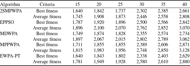
. The number of targets is set at 15, 20, 25, 30, 35 and 40 for comparative testing, with each experiment repeated 50 times, as shown in Figs. 17–22 (Table 6).
The number of targets = 15.

The number of targets = 20.

The number of targets = 25.

The number of targets = 30.

The number of targets = 35.

The number of targets = 40.

Comparative experiments with different numbers of targets

As shown in the previous figures and tables, the proposed algorithm significantly outperforms the comparative algorithms across all metrics. Furthermore, as the problem dimensionality increases, the advantage of the proposed algorithm in solution accuracy becomes more pronounced. Additionally, with the increase in dimensionality, the gap between the average fitness and the best fitness of all algorithms grows larger, indicating that higher dimensionality poses a challenge to the stability of the algorithms. However, among all the comparative algorithms, the proposed algorithm exhibits the smallest difference between the two metrics, which further validates its excellent solution stability in low-dimensional problems.
In the experiments of this chapter, the proposed algorithm demonstrates advantages in both solution accuracy and stability. This is primarily due to the two-stage approach, where the algorithm focuses on optimising the UAV resource allocation in the initial stage. As a result, even with an increase in the number of UAVs, the algorithm is still able to utilise the optimal UAV resources, thereby reducing the fitness value of the algorithm’s solution.
4.2.3 Comparative experiments under high-dimensional problems
Existing swarm intelligence algorithms inevitably encounter the ‘curse of dimensionality’ when addressing high-dimensional problems. This subsection aims to evaluate the algorithm’s performance in solving high-dimensional issues. In the comparative experiments, based on Section 4.2.2, the number of UAVs is increased by a factor of two, while the number of tasks continues to rise, with the target distribution range fixed at
 $[100,300] \times [100,300]$
. The experimental results are presented in Figs. 23–26.
The number of targets = 50.

The number of targets = 60.

The number of targets = 70.

The main objective of the experiments in this chapter is to verify the effectiveness of the proposed algorithm in solving high-dimensional complex problems. The experimental results demonstrate that all the algorithms tested exhibit a certain degree of performance degradation in terms of solution accuracy when handling high-dimensional problems. However, the proposed algorithm is more effective in overcoming the curse of dimensionality, consistently maintaining a leader level of solution accuracy across all experimental scenarios, demonstrating strong stability. This indicates that the proposed algorithm is not only capable of adapting to simple problems but also maintains excellent solution performance when addressing high-dimensional complex problems.
The experimental results are partly attributed to the algorithm’s allocation of a portion of the computational resources specifically for optimising UAV resource utilisation, which allows it to maintain an accuracy advantage even when dealing with high-dimensional complex problems. In addition, the multi-population mechanism proposed in this paper also helps the algorithm escape local optima when addressing high-dimensional complex problem, thereby improving the stability of the solution.
4.3 Visualisation results analysis
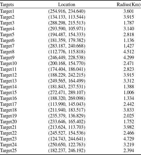
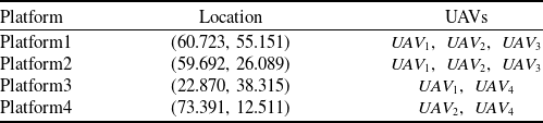
Due to the differences in the solution models, quantitative analysis, while offering some reference value, is not comprehensive. This subsection aims to perform a qualitative analysis of the algorithm through the UAV trajectories obtained by algorithms. In the comparative experiments, the number of UAVs is fixed at 10, while the number of tasks is set at 25. The target position, launch platform locations, and the types of UAVs included in the launch platforms are fixed, as shown in Tables 7 and 8. The final visualisation results are presented in Figs. 27–31.
Targets attributions

The number of targets = 80.

Platforms attributions

The visualisation of the MDWPA algorithm.

The visualisation of the MPPWPA algorithm.

The visualisation of the EPPSO algorithm.

The visualisation of the EWPA-PT algorithm.

The visualisation of the 2SMPWPA algorithm.

As shown in the previous figures, various comparative algorithms inevitably exhibit issues such as entangled flight paths of UAVs (Figs. 27 and 29), excessive flight spans of UAVs (Fig. 28), and wasteful usage of resources (Figs. 27–30). Fig. 31 illustrates the practical solution results of the proposed 2SMPWPA algorithm. As shown, the algorithm not only utilizes the minimum number of UAV resources to complete all the tasks to be allocated, but also generates smoother flight paths, reducing the spatial span of UAVs during their mission execution. Overall, this algorithm demonstrates excellent practicality in solving multi-UAV task allocation problems.
5.0 Conclusion
This study aims to address the issues faced by existing algorithms in solving multi-UAV task allocation problems, specifically the large spatial spans of individual UAV tasks, entangled flight paths and inefficient utilisation of UAV resources. To this end, we propose a 2SMPWPA. This innovative algorithm divides the solution process into two stages: the early stage focuses on optimising the utilisation of UAV resources. In contrast, the latter stage emphasises adjusting the task execution plans based on the existing UAV resources. Additionally, we introduce a dynamic population mechanism, population protection mechanism, population migration mechanism and population communication mechanism and employ a roulette wheel selection method to enhance the individual reconstruction within the wolf pack algorithm. Experimental results demonstrate that the proposed algorithm effectively addresses the aforementioned issues and achieves satisfactory outcomes.
Although the algorithm proposed in this paper offers significant advantages in solution accuracy and effectively enhances the performance of multi-UAV task allocation, the adoption of a two-stage approach inevitably increases the algorithm’s complexity. Therefore, how to effectively reduce the algorithm’s complexity and accelerate its running efficiency while maintaining high accuracy remains a direction for future improvements.
In future work, we will first focus on improving the quality of the initial solution to accelerate the convergence of the algorithm. Enhancing the solution speed of the algorithm is also an important task. Furthermore, UAV task allocation also involves task assignment in dynamic environments, and we will explore the use of deep reinforcement learning strategies to address this issue. Finally, due to the limited onboard computational power of individual UAVs, the solution to multi-UAV task allocation relies on a central system. However, there are significant performance differences among various central systems. In future work, we will conduct more real-world experiments to improve and optimise the algorithm’s performance continuously.
Competing interests
The authors declare none.