1. Introduction
Rayleigh–Bénard (RB) convection is a classical buoyancy-driven flow in astrophysical and geophysical flows (Pedlosky Reference Pedlosky1987), mantle convection (Richter Reference Richter1978; Peltier Reference Peltier1985), chemical vapour deposition (Jensen Reference Jensen1991) and cooling equipment (Zhang, Zou & Fu Reference Zhang, Zou and Fu2023). Under the action of bottom heating and upper cooling, the stationary fluid begins to move when the buoyancy force is greater than the viscous force, and the driving parameter at the linear onset, i.e. the critical Rayleigh number Ra c , is 1707.762 with no-slip and perfectly conducting boundary conditions (Chandrasekhar Reference Chandrasekhar1961). When a shear flow is introduced, the linear threshold of spanwise-uniform disturbances usually increases with increasing Re, the Reynolds number which measures the magnitude of the base flow, while the linear instability of streamwise-uniform disturbances is unaffected (Gallagher & Mercer Reference Gallagher and Mercer1965; Gage & Reid Reference Gage and Reid1968; Nicolas Reference Nicolas2002). In RB convection of Newtonian fluids where the linear operator is normal, energy stability theory indicates that the perturbation energy decays monotonically in time for Ra < Ra c while it grows exponentially for Ra > Ra c , so that the bifurcation of this convection is supercritical and can be predicted precisely by modal stability analysis (Joseph Reference Joseph1965). In wall-bounded shear flows, however, it is difficult to describe the transition scenario accurately by modal theory since the significant algebraic growth of perturbation energy in these flows can lead to the subcritical bifurcation despite of linear stability (Schmid & Henningson Reference Schmid and Henningson2001; Schmid Reference Schmid2007).
1.1. Transient growth of Newtonian shear flows with and without a temperature gradient
In the absence of nonlinear effects, the short-term growth of perturbation kinetic energy is related to the non-normality of the linear operators (Trefethen et al. Reference Trefethen, Trefethen, Reddy and Driscoll1993; Schmid & Henningson Reference Schmid and Henningson2001; Schmid Reference Schmid2007), and this phenomenon was first demonstrated by Boberg & Brosa (Reference Boberg and Brosa1988) in a pipe flow. Mathematically, before the asymptotic instability sets in, even if all the eigenfunctions of control operators decay exponentially with time, the superposition of these eigenfunctions may produce a significant rapid amplification of perturbation energy in a short instant, which provides a perspective for controlling the response behaviour of input perturbations. Modal analysis indicates that plane Couette flow and pipe Poiseuille flow in Newtonian fluids is linearly stable (Romanov Reference Romanov1973; Schmid & Henningson Reference Schmid and Henningson2001) for all Re, but in fact, these flow systems can transition from a laminar state to a turbulent state (Tillmark & Alfredsson Reference Tillmark and Alfredsson1992; Dauchot & Daviaud Reference Dauchot and Daviaud1995). Besides, modal analysis suggests that plane Poiseuille flow is laminar unless Re exceeds 5772.22 to trigger a Tollmien–Schlichting instability while experimental studies showed that Poiseuille flow can transition to turbulence at Re no larger than 1000 (Patel & Head Reference Patel and Head1969; Schmid & Henningson Reference Schmid and Henningson2001; Tao, Chen & Su Reference Tao, Chen and Su2011). Transient energy amplification is instructive to understand the aforementioned differences in the transition from laminar to turbulent flow predicted by the modal stability analysis and observed by experiments (Schmid Reference Schmid2007). Specifically, different from the classical transition of modal path, e.g. Tollmien–Schlichting waves, sufficiently large transient energy amplification can trigger nonlinear instability by the generation of high-speed streaks thus leading to another transition scenario, i.e. the bypass transition (Klebanoff, Tidstrom & Sargent Reference Klebanoff, Tidstrom and Sargent1962). In addition, non-modal analysis also can provide insights into structural features of turbulent flows (Hwang & Cossu Reference Hwang and Cossu2010a ,Reference Hwang and Cossu b ) and may offer an amplification mechanism that causes a self-sustained nonlinear state (Thomas et al. Reference Thomas, Lieu, Jovanović, Farrell, Ioannou and Gayme2014).
The Orr mechanism and the lift-up mechanism are responsible for the transient energy growth in parallel shear flows (Butler & Farrell Reference Butler and Farrell1992; Schmid & Henningson Reference Schmid and Henningson2001; Brandt Reference Brandt2014). In two-dimensional flows, the optimal initial velocity perturbation is inclined against the mean shear flow in structure, and subsequently this structure tilts into the mean shear direction. When the perturbation tilts downstream, the interaction between the different fluid velocity layers causes the energy from the base flow field to transfer to the perturbed hydrodynamic field, resulting in transient growth. This process is referred to as the Orr mechanism. In three-dimensional flows, streamwise vortices drive low-energy fluids near the boundaries into regions of faster mean flow so as to form streamwise streaks, thus causing the energy release from the mean shear to the perturbed wall-normal vorticity. This energy growth process is referred to as the lift-up mechanism. In the high-Re regime, energy growth caused by the lift-up mechanism is generally greater than that caused by the Orr mechanism (Trefethen et al. Reference Trefethen, Trefethen, Reddy and Driscoll1993; Schmid & Henningson Reference Schmid and Henningson2001).
In RB–Poiseuille/Couette mixed convection of Newtonian fluids, transient energy growth also exists, which is also due to the Orr and lift-up mechanisms. The temperature gradient has a non-trivial influence on this growth (Sameen & Govindarajan Reference Sameen and Govindarajan2007), where heat diffusivity and unstable density stratification play an important role, but viscosity stratification has little effect. Similar to the pure bounded shear flows, (nearly) streamwise-uniform disturbances in plane Poiseuille (Couette) flow can reach the largest transient energy growth in the presence of an unstable temperature gradient, which is enhanced when increasing buoyancy or decreasing the viscosity (Jerome, Chomaz & Huerre Reference Jerome, Chomaz and Huerre2012). When a stable temperature gradient is imposed on bounded shear flows, the lift-up mechanism will be inhibited due to the inhibition of vertical motions (Eaves & Caulfield Reference Eaves and Caulfield2015) while the Orr mechanism is unaffected. As a result, oblique disturbances will have the largest transient growth (Biau & Bottaro Reference Biau and Bottaro2004; Jose et al. Reference Jose, Roy, Bale, Lyer and Govindarajan2018).
1.2. Effects of viscoelasticity on transient growth of bounded shear flow
As one of the non-Newtonian fluids, viscoelastic fluids not only exist widely in nature (such as muds, blood, mantle, polymer solution, etc.), but are also widely used in industry due to their special properties, such as enhancing fluid mixing (Groisman & Steinberg Reference Groisman and Steinberg2001), energy storage (Kang et al. Reference Kang, Kim, Song, Hong, Kim, Goh, Chung and Lee2023), heat transport enhancement (Boffetta et al. Reference Boffetta, Mazzino, Musacchio and Vozella2010) and drag reduction (White & Mungal Reference White and Mungal2008; Xi Reference Xi2019). Viscoelastic effects of fluid are characterized by the viscosity ratio and elastic number; the former describes the solvent to solution viscosity while the latter denotes the relative magnitude of viscoelastic and inertial effects. In plane Poiseuille/Couette flow of viscoelastic fluids where streamwise elongated structures, i.e. streamwise streaks, generally have the largest energy growth, increasing the elasticity number or decreasing the viscosity ratio can significantly enhance the energy amplification, with the optimal spanwise wavenumber to achieve the maximum energy amplification increasing simultaneously (Hoda, Jovanović & Kumar Reference Hoda, Jovanović and Kumar2008). Specifically, it is found that the energy exchange between the streamwise/wall-normal component of polymeric stresses and the wall-normal gradient of the streamwise velocity (Hoda, Jovanović & Kumar Reference Hoda, Jovanović and Kumar2009) is responsible for the enhancement of the transient growth. The direct numerical simulation by Ibarra & Park (Reference Ibarra and Park2023) confirms the enhancement of viscoelasticity on transient growth of bounded shear flows. Considering viscoelastic fluids of dilute polymer concentration and low elasticity, Ibarra & Park (Reference Ibarra and Park2023) studied the early linear non-modal behaviour and later nonlinear dynamics during the laminar–turbulent transition. Compared with the Newtonian case, they found that the fluid viscoelasticity acts to accelerate the formation of quasistreamwise vortices around low-speed streaks so that a faster transition to turbulence is observed. Besides, similar to the Newtonian cases, the critical perturbation amplitude is proportional to Re −1.25. It should be noted that viscoelasticity cannot always lead to the enhancement of non-modal instability if one considers the oblique disturbances, see, for instance, Zhang et al. (Reference Zhang, Lashgari, Zaki and Brandt2013).
The studies mentioned above tried to understand the subcritical bifurcation of bounded viscoelastic shear flows to the inertial turbulence. However, it is noted that different from the Newtonian fluids, the viscoelastic channel flow with high fluid elasticity also can transition to the turbulent state at low or even zero Re, and the generated turbulence in this case is called the elastic turbulence (Steinberg Reference Steinberg2021; Datta et al. Reference Datta2022; Dubief, Terrapon & Hof Reference Dubief, Terrapon and Hof2023). In this regard, it is found that the inertialess plane Poiseuille/Couette flow of Oldroyd-B fluid is able to generate significant transient growth due to the interactions between the polymeric stresses fluctuations and the background shear (Jovanović & Kumar Reference Jovanović and Kumar2010, Reference Jovanović and Kumar2011; Lieu, Jovanović & Kumar Reference Lieu, Jovanović and Kumar2013). Specifically, the background shear stretches the polymer to generate alternating regions of relatively high/low streamwise velocity, which bears a strong resemblance to vortex tilting by the lift-up mechanism in inertia-dominant bounded shear flows. During this elasticity-dominant transient growth, wall-normal and spanwise forces have the greatest impact on flow fluctuations and among these flow fluctuations, the fluctuations in streamwise velocity and the streamwise component of the polymeric stresses tensor are the most affected (Jovanović & Kumar Reference Jovanović and Kumar2011). In addition, the Weissenberg number W representing the ratio of the polymer relaxation time and the flow convective time acts as a driving parameter like the Reynolds number (Jovanović & Kumar Reference Jovanović and Kumar2010), with the perturbed kinetic energy and the perturbed elastic energy scaling as W 2 and W 4, respectively (Lieu et al. Reference Lieu, Jovanović and Kumar2013). It is believed that the aforementioned non-modal behaviour can be a plausible mechanism for the initiation of elastic turbulence through the bypass transition in viscoelastic channel flows. This is evidenced by a recent experimental study of Shnapp & Steinberg (Reference Shnapp and Steinberg2022) who observed the algebraic growth of normalized root-mean squared streamwise velocity/pressure fluctuations. After the algebraic growth, characteristic patterns such as elastic waves and the viscoelastic analogue of streamwise streaks persisting in the long term arise.
As shown above, while many works have confirmed that the viscoelasticity and temperature gradient have significant influences on the transient growth of bounded shear flows, the combined effects of these two factors on the non-modal instability of bounded shear flows have not been resolved. Specifically, due to the competition between polymer relaxation time and thermal diffusion time, the imposing of a temperature gradient into a viscoelastic fluid can cause a transition from the stationary instability to the oscillatory instability when the elastic effects are sufficiently intense (Vest & Arpaci Reference Vest and Arpaci1969). In addition to this instability transition, the superposition of viscoelasticity and temperature gradient can also yield the transition from the absolute instability to the convective instability (see the spatiotemporal analysis by Hirata et al. (Reference Hirata, Alves, Delenda and Ouarzazi2015)) and the transition from the supercritical bifurcation to the subcritical bifurcation (see the Hopf bifurcation analysis by Park & Lee (Reference Park and Lee1996)). Therefore, it is necessary to examine the combined effects of viscoelasticity and temperature gradient on the transient growth of wall-bounded shear flows, which is the main aim of the present study. Many theoretical studies have demonstrated that the superposition of unstable temperature gradient and fluid viscoelasticity can indeed generate oscillatory convection and the computational results presented below are consistent with this finding, but it is still challenging to confirm this point experimentally (Larson Reference Larson1992). For instance, while Kolodner (Reference Kolodner1998) and Métivier et al. (Reference Métivier, Brochard, Darbouli and Magnin2020) successfully observed oscillatory convection in experiments, they could not determine whether it was driven by the interaction between the unstable temperature gradient and viscoelasticity or by other factors, such as the Soret effect or stick–slip boundary effect.
In this study, to have a better understanding of the combined effects of an unstable temperature gradient and the viscoelasticity on the transient growth of bounded shear flows, we shall first investigate the non-modal instability of pure RB convection in viscoelastic fluids and then examine the transient growth in the presence of a shear at low and high Re regimes, respectively. We shall consider Oldroyd-B fluids and to obtain a comprehensive view, both plane Couette flow and Poiseuille flow will be included. The remainder of this paper is organized as follows. In § 2, the governing equations and non-modal analysis method are introduced based on the Oldroyd-B fluids. We first systematically investigate the non-modal effects induced by the viscoelasticity and temperature gradient in § 3, and then in § 4, the combined effects of viscoelasticity and temperature gradient on the transient growth of both Poiseuille flow and Couette flow are discussed. Finally, we conclude the main findings in § 5.
2. Problem formulation
2.1. Mathematical modelling and governing equations
Figure 1 shows the schematic of RB convection with and without bounded shear flows in viscoelastic fluids. The upper and lower plates extend infinitely in x (streamwise) and z (spanwise) directions, and maintain constant lower and higher temperatures, respectively. Three baseflow configurations are considered, i.e. hydrostatic state, Poiseuille flow and Couette flow. Regarding the viscoelastic effects, we consider the Oldroyd-B fluid since it focuses on the interaction between polymers and hydrodynamic fluctuations (Zhang et al. Reference Zhang, Zhang, Wang, Li, Yu and Li2022) and can capture the essential instability mechanism in the flow (e.g. centre mode instability in Garg et al. (Reference Garg, Chaudhary, Khalid, Shankar and Subramanian2018)).
Schematic description of the problem.

It is assumed that the flow is incompressible and the Oberbeck–Boussinesq approximation (Chandrasekhar Reference Chandrasekhar1961) holds. Therefore, the governing equations are
 \begin{align} &\nabla ^{*}\cdot \boldsymbol{U}^{*}=0, \end{align}
 \begin{align} \rho ^{*}\frac{\partial \boldsymbol{U}^{*}}{\partial t^{*}}+\rho ^{*}\left(\boldsymbol{U}^{*}\cdot \nabla ^{*}\right)\boldsymbol{U}^{*}&=-\nabla ^{*}P^{*}+\nabla ^{*}\cdot \boldsymbol{\tau }^{*}+\rho ^{*}g^{*}\zeta ^{*}\left(\Theta ^{*}-\Theta _{1}^{*}\right)\mathbf{1}_{y}\,, \end{align}
 \begin{align} \left(\frac{\partial \Theta ^{*}}{\partial t^{*}}+\boldsymbol{U}^{*}\cdot \nabla ^{*}\Theta ^{*}\right)&=\nabla ^{*}\cdot \left(\kappa ^{*}\nabla ^{*}\Theta ^{*}\right),\end{align}
 \begin{align} \boldsymbol{\tau }^{*}&=\boldsymbol{\tau }_{s}^{*}+\boldsymbol{\tau }_{p}^{*}\,, \end{align}
 \begin{align} \boldsymbol{\tau }_{s}^{*}&=\mu _{s}^{*}\big[\nabla ^{*}\boldsymbol{U}^{*}+(\nabla ^{*}\boldsymbol{U}^{*})^{T}\big], \end{align}
 \begin{align} \boldsymbol{\tau }_{p}^{*}+\lambda ^{*}(\boldsymbol{\tau }_{p}^{*})^{\nabla }&=\mu _{p}^{*}\big[\nabla ^{*}\boldsymbol{U}^{*}+(\nabla ^{*}\boldsymbol{U}^{*})^{T}\big], \end{align}
where
U
* is the velocity field, ρ* the density,
P
* the pressure,
τ
* the total stress tensor in viscoelastic fluid, g* the acceleration of gravity, ζ* the thermal expansion coefficient,
 $ \boldsymbol{\unicode{x03C4}}^{\ast}_{{s}}$
the solvent contribution in
τ
*, Θ* the temperature, κ* the thermal diffusivity,
 $ \boldsymbol{\unicode{x03C4}}^{\boldsymbol{\ast}}_{\boldsymbol{p}}$
the polymer contribution in
τ
*,
 $ \mu^{\ast}_{{s}}$
the viscosity of the solvent,
 $ \mu^{\ast}_{{p}}$
the viscosity of the polymer, λ* the relaxation time of the polymer molecules and superscript
T
denotes the transpose of tensor ∇*
U
*.
Here (
 $ \boldsymbol{\unicode{x03C4}}^{\boldsymbol{\ast}}_{\boldsymbol{p}}$
)∇ is the upper-convected time derivative, defined by Larson (Reference Larson1988),
 \begin{equation} (\boldsymbol{\tau }_{p}^{*})^{\nabla }=\frac{\partial \boldsymbol{\tau }_{p}^{*}}{\partial t^{*}}+\nabla ^{*}\cdot (\boldsymbol{U}^{*}\boldsymbol{\tau }_{p}^{*})-(\nabla ^{*}\boldsymbol{U}^{\boldsymbol{*}})^{T}\cdot \boldsymbol{\tau }_{p}^{*}-\boldsymbol{\tau }_{p}^{*}\cdot \nabla ^{*}\boldsymbol{U}^{\boldsymbol{*}}. \end{equation}
Substituting (2.2) into (2.1f ), we have
 \begin{equation} \boldsymbol{\tau }_{p}^{*}\!+\!\lambda ^{*}\left(\frac{\partial \boldsymbol{\tau }_{p}^{*}}{\partial t^{*}}\!+\!\nabla ^{*}\cdot (\boldsymbol{U}^{*}\boldsymbol{\tau }_{p}^{*})-(\nabla ^{*}\boldsymbol{U}^{\boldsymbol{*}})^{T}\cdot \boldsymbol{\tau }_{p}^{*}-\boldsymbol{\tau }_{p}^{*}\cdot \nabla ^{*}\boldsymbol{U}^{\boldsymbol{*}}\right)\!=\!\mu _{p}^{*}\left[\nabla ^{*}\boldsymbol{U}^{*}+(\nabla ^{*}\boldsymbol{U}^{*})^{T}\right]. \end{equation}
According to Bird et al. (Reference Bird, Curtiss, Armstrong and Hassager1987) and Zhang et al. (Reference Zhang, Lashgari, Zaki and Brandt2013), we have
 \begin{equation} \boldsymbol{\tau }_{p}^{*}=\frac{\mu _{p}^{*}h}{\lambda ^{*}k_{B}\Theta ^{*}}(\boldsymbol{C}^{*}-\boldsymbol{C}^{*eq}),\quad \boldsymbol{C}^{*eq}=\frac{k_{B}\Theta ^{*}}{h},\quad\boldsymbol{\tau }_{p}^{*}=\frac{\mu _{p}^{*}}{\lambda ^{*}}\left(\boldsymbol{C}-\boldsymbol{I}\right), \end{equation}
where h is the spring constant of the elastic dumbbell, k B the Boltzmann constant and C * the conformation tensor.
2.2. Non-dimensionalized governing equations
To non-dimensionalize the governing equations above, we introduce the following scalings:
 \begin{align} \left(x,y,z\right)&=\frac{\left(x^{*},y^{*},z^{*}\right)}{H^{*}},\boldsymbol{U}=\frac{\boldsymbol{U}^{*}}{U_{0}^{*}},t=t^{*}/\left(\frac{H^{*}}{U_{0}^{*}}\right),P=\frac{P^{*}}{\rho ^{*}U_{0}^{*^{2}}},\\ \nonumber \boldsymbol{\tau }_{p}&=\boldsymbol{\tau }_{p}^{*}/\left(\frac{\mu _{p}^{*}U_{0}^{*}}{H^{*}}\right),\boldsymbol{C}=\boldsymbol{C}^{*}/\left(\frac{k_{B}\Theta ^{*}}{h}\right),\Theta =\frac{\Theta ^{*}-\Theta _{1}^{*}}{\Theta _{0}^{*}-\Theta _{1}^{*}}, \end{align}
where
 $ U^{\ast}_{0}$
= (g*ζ*H*
 $\varDelta$
Θ*)0.5 for the hydrostatic case, and
 $ U^{\ast}_{0}$
= U
max
for the sheared cases. The use of these two velocity scalings does not affect the value of instability threshold and transient growth.
After non-dimensionalization, (2.1)–(2.4) read
 \begin{align} &\nabla \cdot \boldsymbol{U}=0, \end{align}
 \begin{align} \frac{\partial \boldsymbol{U}}{\partial t}+\left(\boldsymbol{U}\cdot \nabla \right)\boldsymbol{U}=-\nabla P&+\frac{\beta }{Re}\nabla ^{2}\boldsymbol{U}+\frac{1-\beta }{Re^{2}E}\nabla \cdot \boldsymbol{C}\mathbf{+}\frac{Ra}{Re^{2}Pr}\Theta \mathbf{1}_{\boldsymbol{y}}\,, \end{align}
 \begin{align} \frac{\partial \Theta }{\partial t}+\boldsymbol{U}\cdot \nabla \Theta & =\frac{1}{RePr}\nabla ^{2}\Theta,\end{align}
 \begin{align} \frac{\partial \boldsymbol{C}}{\partial t}+\boldsymbol{U}\cdot \nabla \boldsymbol{C}-\boldsymbol{C}\cdot \nabla \boldsymbol{U}&-\left(\nabla \boldsymbol{U}\right)^{T}\cdot \boldsymbol{C}=-\frac{\boldsymbol{C}-\boldsymbol{I}}{ReE},\end{align}
where
 \begin{equation} Re=\frac{\rho ^{*}U_{0}^{*}H^{*}}{\mu ^{*}}, Ra=\frac{g^{*}\zeta ^{*}(\Theta _{0}^{*}-\Theta _{1}^{*})H^{{*^{3}}}}{\kappa ^{*}\nu ^{*}}, Pr=\frac{\nu ^{*}}{\kappa ^{*}}, \beta =\frac{\mu _{s}^{*}}{\mu ^{*}}, E=\frac{\lambda ^{*}\mu ^{*}}{\rho ^{*}H^{{*^{2}}}}. \end{equation}
Here, Re is Reynolds number which measures the relative importance of the inertia force to the viscous force. The Rayleigh number Ra represents the ratio between buoyancy force and viscous force. The Prandtl number Pr is the ratio between the kinematic viscosity and the thermal diffusion coefficient. Here β is viscosity ratio, defined as the ratio of the solvent viscosity to the total viscosity. Here E is elasticity number, which measures the magnitude of elasticity in a viscoelastic fluid. Besides, the kinematic viscosity is defined as ν* = μ*/ρ*, and the total dynamic viscosity is defined as μ* =
 $ \mu^{\ast}_{{s}} + \mu^{\ast}_{{p}}$
.
The dimensionless boundary conditions are Θ(−1) = 1, Θ(1) = 0, U(±1) = 0 for the hydrostatic case and Poiseuille flow, and U(1) = 1, U(−1) = -1 for Couette flow, where the vertical distance y
 $\in$
[−1,1] after non-dimensionalization.
2.3. Linear stability problem
We decompose the flow variable into the sum of the base state and perturbation, i.e.
 $\boldsymbol{U}=\overline{\boldsymbol{U}}+u, P=\overline{P}+p, \Theta =\overline{\Theta}+\theta$
and
 $\boldsymbol{C}=\overline{\boldsymbol{C}}+c$
, where the uppercase letters with a horizontal above represent the base state quantity and the lowercase letters are perturbations. After substituting these decompositions into (2.6), the linear system reads
 \begin{equation} \nabla \cdot \boldsymbol{u}=0, \end{equation}
 \begin{equation} \frac{\partial \boldsymbol{u}}{\partial t}+\left(\boldsymbol{u}\cdot \nabla \right)\overline{\boldsymbol{U}}+\left(\overline{\boldsymbol{U}}\cdot \nabla \right)\boldsymbol{u}=-\nabla p+\frac{\beta }{Re}\nabla ^{2}\boldsymbol{u}+\frac{1-\beta }{Re^{2}E}\nabla \cdot \boldsymbol{c}+\frac{Ra}{Re^{2}Pr}\theta \mathbf{1}_{\boldsymbol{y}}\,, \end{equation}
 \begin{equation} \frac{\partial \theta }{\partial t}+\overline{\boldsymbol{U}}\cdot \nabla \theta +\boldsymbol{u}\cdot \nabla \overline{\Theta}=\frac{1}{RePr}\nabla ^{2}\theta, \end{equation}
 \begin{equation} \frac{\partial \boldsymbol{c}}{\partial t}+\overline{\boldsymbol{U}}\cdot \nabla \boldsymbol{c}+\boldsymbol{u}\cdot \nabla \overline{\boldsymbol{C}}-\overline{\boldsymbol{C}}\cdot \nabla \boldsymbol{u}-\boldsymbol{c}\cdot \nabla \overline{\boldsymbol{U}}-\left(\nabla \boldsymbol{u}\right)^{T}\cdot \boldsymbol{C}-\left(\nabla \overline{\boldsymbol{U}}\right)^{T}\cdot \boldsymbol{c}=-\frac{\boldsymbol{c}}{ReE}, \end{equation}
with the accompanying boundary conditions being u(±1) = 0 and θ(±1) = 0.
Based on (2.6), the base-state velocity field is
 $\overline{\boldsymbol{U}}=0$
(hydrostatic state),
 $\overline{\boldsymbol{U}}=1-y^{2}$
(Poiseuille flow) and
 $\overline{\boldsymbol{U}}=y$
(Couette flow), and the base temperature field is
 $\overline{\Theta}=\mathrm{0}.\mathrm{5}(1-y)$
. Moreover, the base conformation tensor is
 \begin{equation} \overline{C}=\left(\begin{array}{c@{\quad}c@{\quad}c} 2\left(ReE\right)^{2}\overline{U}^{\prime 2}+1 & ReE\overline{U}' & 0\\ ReE\overline{U}' & 1 & 0\\ 0 & 0 & 1 \end{array}\right). \end{equation}
Since the flow is homogeneous in the streamwise and spanwise directions, it is assumed that the perturbations are wave-like (periodic in these two directions), i.e.
 \begin{equation} \boldsymbol{f}\left(x,y,z,t\right)=\,\tilde{\!\boldsymbol{f}}\left(y,t\right)e^{\left(i\alpha x+i\gamma z\right)}=\,\hat{\!\boldsymbol{f}}\left(y\right)e^{-i\omega t}e^{\left(i\alpha x+i\gamma z\right)}, \end{equation}
where
f
can be an arbitrary perturbation, the real-valued α and γ are streamwise and spanwise wavenumbers, respectively,
 $\,\tilde{\!\boldsymbol{f}}$
and
 $\,\hat{\!\boldsymbol{f}}$
are the shape functions and ω is the complex circular frequency of disturbance, with its imaginary part ω
i
representing the growth rate of linear disturbance (if ω
i
> 0, the fluid system is linearly unstable, and ω
i
< 0 indicates the stable flow). Using the wall-normal vorticity η = ∂u/∂z – ∂w/∂x to eliminate the pressure term, we get
 \begin{equation} \boldsymbol{A}\frac{\partial }{\partial t}\tilde{\boldsymbol{\chi }}=\boldsymbol{B}\tilde{\boldsymbol{\chi }}, \end{equation}
where
 $\tilde{\boldsymbol{\chi }}= (\tilde{{v}},\tilde{{\eta }},\tilde{\theta },\tilde{{c}}_{11},\tilde{{c}}_{22},\tilde{{c}}_{33},\tilde{{c}}_{12},\tilde{{c}}_{13},\tilde{{c}}_{23})$
T, and the elements in matrices
A
and
B
can be easily deduced from (A1)–(A9) in Appendix A.
For modal analysis, (2.11) can be further simplified as
 \begin{equation} -i\omega \hat{\boldsymbol{\chi }}=\boldsymbol{L}\hat{\boldsymbol{\chi }}, \end{equation}
where L = A −1 B , since matrix A is invertible, and the linear modal question becomes an eigenvalue problem.
2.4. Energy norm and input–output non-modal analysis
To predict the transient evolution of perturbation, we transform the eigenvalue problem (2.12) into an initial value problem, i.e.
 \begin{equation} \frac{\partial \tilde{\boldsymbol{\chi }}}{\partial t}=\boldsymbol{L}\tilde{\boldsymbol{\chi }}. \end{equation}
In this study, we focus on the non-modal instability related to the inertial turbulence instead of the elastic turbulence. Therefore, we only consider the temporal evolution of the perturbed kinetic energy and thermal energy but neglect the elastic energy stored in polymers. The case that polymer disturbances are input directly and elastic potential energy is defined is discussed in Appendix D. Following Hoda et al. (Reference Hoda, Jovanović and Kumar2008), Zhang et al. (Reference Zhang, Lashgari, Zaki and Brandt2013) and Ibarra & Park (Reference Ibarra and Park2023), at the initial time t = 0+, the polymer is not perturbed directly but indirectly forced through Hamiltonian operator ∇. In this case, the energy norm is defined as
 \begin{equation} \int _{{\Omega} }\varepsilon {\mathrm{d}}V=\frac{1}{2}\times \frac{1}{2}\int _{{\Omega} }(A_{1}(\left| \tilde{u}\right| ^{2}+\left| \tilde{{v}}\right| ^{2}+| \tilde{w}| ^{2})+A_{2}| \tilde{\theta }| ^{2}){\mathrm{d}}y=\int _{{\Omega} }\tilde{\boldsymbol{\chi }}^{\dagger }\boldsymbol{M}\tilde{\boldsymbol{\chi }}{\mathrm{d}}y, \end{equation}
where
 $\unicode{x1D6FA}$
= 2ab, a = 2π/α, b = 2π/γ, and the superscript † stands for the conjugate transpose. In addition, A
1 = 1, and A
2 = Ra/(Re
2
Pr) (Sameen & Govindarajan Reference Sameen and Govindarajan2007; Jerome et al. Reference Jerome, Chomaz and Huerre2012).
The details of the energy weight matrix M are given as
 \begin{equation} \boldsymbol{M}=\frac{1}{4}diag\left(\boldsymbol{I}+\frac{1}{k^{2}}\boldsymbol{D}_{1}^{\dagger }\boldsymbol{D}_{1},\frac{1}{k^{2}}\boldsymbol{I},\frac{Ra}{Re^{2}Pr}\boldsymbol{I},\boldsymbol{Z},\boldsymbol{Z},\boldsymbol{Z},\boldsymbol{Z},\boldsymbol{Z,Z}\right), \end{equation}
where I denotes a N× N identity matrix, Z a N× N zero matrix, k 2 = α 2 + γ 2 and D 1 the first-derivation matrix with respect to the vertical direction y.
Applying a Cholesky decomposition to the weight matrix M , i.e.
 \begin{equation} \boldsymbol{M}=\boldsymbol{F}^{\dagger }\boldsymbol{F} \end{equation}
and defining
 $\tilde{\boldsymbol{\xi }}=\boldsymbol{F}\tilde{\boldsymbol{\chi }}$
, we arrive at
 \begin{equation} \int _{{\Omega} }\varepsilon {\mathrm{d}}V=\int _{{\Omega} }\tilde{\boldsymbol{\chi }}^{\dagger }\boldsymbol{M}\tilde{\boldsymbol{\chi }}{\mathrm{d}}y=\int _{\Omega }\tilde{\boldsymbol{\chi }}^{\dagger }\boldsymbol{F}^{\dagger }\boldsymbol{F}\tilde{\boldsymbol{\chi }}{\mathrm{d}}y=\int _{\Omega }\tilde{\boldsymbol{\xi }}^{\dagger }\tilde{\boldsymbol{\xi }}{\mathrm{d}}y=\left\| \tilde{\boldsymbol{\xi }}\right\| _{2}^{2}\,, \end{equation}
where || · ||2 represents the L 2-norm.
To perform the input–output analysis, the input filter
B
in
and the output filter
C
out
should be defined. The input initial condition is
 $\tilde{\boldsymbol{\chi }}$
in
=
B
in
 $\tilde{\boldsymbol{\chi }}^0_{in}$
(t = 0) and the output is
 $\tilde{\boldsymbol{\chi }}$
out
=
C
out
 $\tilde{\boldsymbol{\chi }}^0_{out}$
, where
 $\tilde{\boldsymbol{\chi }}^0_{out}$
= e
t
L
 $\tilde{\boldsymbol{\chi }}$
in
= e
t
L
B
in
 $\tilde{\boldsymbol{\chi }}^0_{in}$
(t = 0). Therefore, the output becomes
 $\tilde{\boldsymbol{\chi }}$
out
=
C
out
 $\tilde{\boldsymbol{\chi }}^0_{out}$
=
C
out
e
t
L
B
in
 $\tilde{\boldsymbol{\chi }}^0_{in}$
(t = 0).
We redefine the output energy weight matrix
M
out
=
C
out
 $\boldsymbol{MC}^{T}_{out}$
and the input energy weight matrix
M
in
=
 $\boldsymbol{B}^{T}_{in}$
MB
in
. Reapplying a Cholesky decomposition to
M
in
and
M
out
:
M
in
=
 $\boldsymbol{F}^{\dagger}_{in}$
F
in
,
M
out
=
 $\boldsymbol{F}^{\dagger}_{out}$
F
out
, the maximum energy growth over all initial conditions with an input–output matrix is
 \begin{equation} \begin{array}{ll} G\left(t\right) & =\max\limits_{\tilde{\boldsymbol{\xi }}_{in}^{0}(t\,=\,0)}\frac{\left\| \tilde{\boldsymbol{\xi }}_{out}\left(t\right)\right\| _{2}^{2}}{\left\| \tilde{\boldsymbol{\xi }}_{in}^{0}(t\,=\,0)\right\| _{2}^{2}}=\max\limits _{\tilde{\boldsymbol{\chi }}_{in}^{0}(t\,=\,0)}\frac{\left\| \boldsymbol{F}_{out}\tilde{\boldsymbol{\chi }}_{out}\left(t\right)\right\| _{2}^{2}}{\left\| \boldsymbol{F}_{in}\tilde{\boldsymbol{\chi }}_{in}^{0}(t\,=\,0)\right\| _{2}^{2}}\\ &=\max\limits _{\tilde{\boldsymbol{\chi }}_{in}^{0}(t\,=\,0)}\frac{\left\| \boldsymbol{F}_{out}\boldsymbol{C}_{out}e^{t\boldsymbol{L}}\boldsymbol{B}_{in}\tilde{\boldsymbol{\chi }}_{in}^{0}(t\,=\,0)\right\| _{2}^{2}}{\left\| \boldsymbol{F}_{in}\tilde{\boldsymbol{\chi }}_{in}^{0}(t\,=\,0)\right\| _{2}^{2}}\\ & =\max\limits _{\tilde{\boldsymbol{\chi }}_{in}^{0}(t\,=\,0)}\frac{\left\| \boldsymbol{F}_{out}\boldsymbol{C}_{out}e^{t\boldsymbol{L}}\boldsymbol{B}_{in}\boldsymbol{F}_{in}^{-1}\boldsymbol{F}_{in}\tilde{\boldsymbol{\chi }}_{in}^{0}(t\,=\,0)\right\| _{2}^{2}}{\left\| \boldsymbol{F}_{in}\tilde{\boldsymbol{\chi }}_{in}^{0}(t\,=\,0)\right\| _{2}^{2}}=\left\| \boldsymbol{F}_{out}\boldsymbol{C}_{out}e^{t\boldsymbol{L}}\boldsymbol{B}_{in}\boldsymbol{F}_{in}^{-1}\right\| _{2}^{2}\, . \end{array} \end{equation}
The maximum value on the G(t) curve is defined as G max , and the input initial condition that reaches this peak G max is the optimal initial condition. The transient growths (of all disturbances) corresponding to different initial conditions are defined in table 1, while the transient growths of various energy components are defined in table 2. It is easy to know the expression of various B in and C out , see, for instance, Zhang et al. (Reference Zhang, Martinelli, Wu, Schmid and Quadrio2015).
The definition of input filters and the definition of its resulting transient growth, with C out fixed as C out4.

The definition of output filters and the definition of its resulting transient growth, with B in fixed as B in4.

According to Schmid & Henningson (Reference Schmid and Henningson2001), using singular value decomposition, the first column of T is extracted as the optimal initial condition and the first column of R is the optimal response, i.e.
 \begin{equation}\boldsymbol{F}_{out}\boldsymbol{C}_{out}e^{{t_{\textit{max} }}\boldsymbol{L}}\boldsymbol{B}_{in}\boldsymbol{F}_{in}^{-1}=\boldsymbol{R}\sum \boldsymbol{T}^{\dagger}\rightarrow \boldsymbol{F}_{out}\boldsymbol{C}_{out}e^{{t_{\textit{max} }}\boldsymbol{L}}\boldsymbol{B}_{in}\boldsymbol{F}_{in}^{-1}\boldsymbol{T}=\boldsymbol{R}\sum \end{equation}
where t max is the time to reach G max .
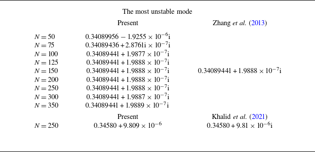
The numerical methods and code validation can be found in Appendix C.
3. Non-modal stability analysis of the pure RB convection in viscoelastic fluids
In this section, the non-modal instability of viscoelastic RB convection in the absence of shear flows is investigated, which will be confirmed to be significantly different from the one singly due to the viscoelasticity, i.e. the elastic non-modal growth examined by Jovanović & Kumar (Reference Jovanović and Kumar2010). We consider α ≠ 0, γ = 0 due to the horizontal symmetry of the problem. To start, we first show in figure 2 the critical Rayleigh number Ra c and the critical streamwise wavenumber α c as a function of the elasticity number E. When E is small, it has no influence on Ra c and α c . Once E exceeds a critical value E c , however, a sudden jump of α c occurs and after that Ra c and α c become a decreasing function of E. This transition marks the occurrence of a Hopf bifurcation distinguishing the weakly elastic regime in which the instability is stationary and the strongly elastic regime in which the instability is oscillatory (Li & Khayat Reference Li and Khayat2005; Hirata et al. Reference Hirata, Alves, Delenda and Ouarzazi2015; Alves, Hirata & Ouarzazi Reference Alves, Hirata and Ouarzazi2016). Under the parameters considered in figure 2, E c = 8.20612.
Critical Rayleigh number Ra c and critical streamwise wavenumber α c as a function of elasticity number E, and the other parameters are β = 0.75, Pr = 10 and γ = 0.

Let us consider two elastic numbers near E c , i.e. E = 8 and E = 8.4 which correspond to the stationary instability and oscillatory instability, respectively. In the stationary instability regime, as shown in figure 3(a), the real part of the most unstable mode is equal to 0, i.e. ω r = 0, indicating the oscillation frequency and propagation speed (i.e. ω r /α) of the perturbation is 0. In this case, the temporal evolution of perturbation energy, shown in figure 3(b), evolves smoothly with time, with the slope in the asymptotic limit equal to the growth rate of the least stable mode, i.e. k G = ω i . Interestingly, unlike the Newtonian RB convection in which the disturbance energy decays monotonically as long as ω i < 0 (Joseph Reference Joseph1965), here one observes a rapid growth of disturbance energy at the early state even the overall energy decays asymptotically. Apparently, it is the inclusion of viscoelasticity that causes the transient growth of perturbation energy.
In stationary instability regime for (a) eigenspectrum and (b) transient energy growth. The parameters are Ra = Ra c = 213.47025, α = α c = 1.558, β = 0.75, E = 8, γ = 0 and Pr = 10. In (b), two additional cases with Ra = 100.015 % Ra c and 99.985 % Ra c are shown for comparison.

The case in the oscillatory instability regime is shown in figure 4(a). In this case, there are two least stable modes that acquire identical imaginary parts but opposite real parts, indicating that their propagation velocities are the same but the propagation directions are opposite. From figure 4(b), it is seen that in addition to the initial transient growth, the disturbance energy oscillates periodically with time. However, with the increase in Ra, the oscillation period increases, and after the transition from oscillatory instability to stationary instability, the oscillation period becomes infinite and the oscillatory behaviour disappears, see the case at Ra = 1.016Ra c in figure 4(b). This small Ra range, i.e. Ra c < Ra< 1.016Ra c , may be one of the reasons why it is difficult to observe oscillatory convection experimentally.
As with figure 3 but in oscillatory instability regime. The other parameters are Ra = Ra c = 212.282, α = α c = 1.69415, β = 0.75, E = 8.4, γ = 0 and Pr = 10. Note that the right-hand ordinate in (b) is used for the case of Ra = 1.016Ra c .

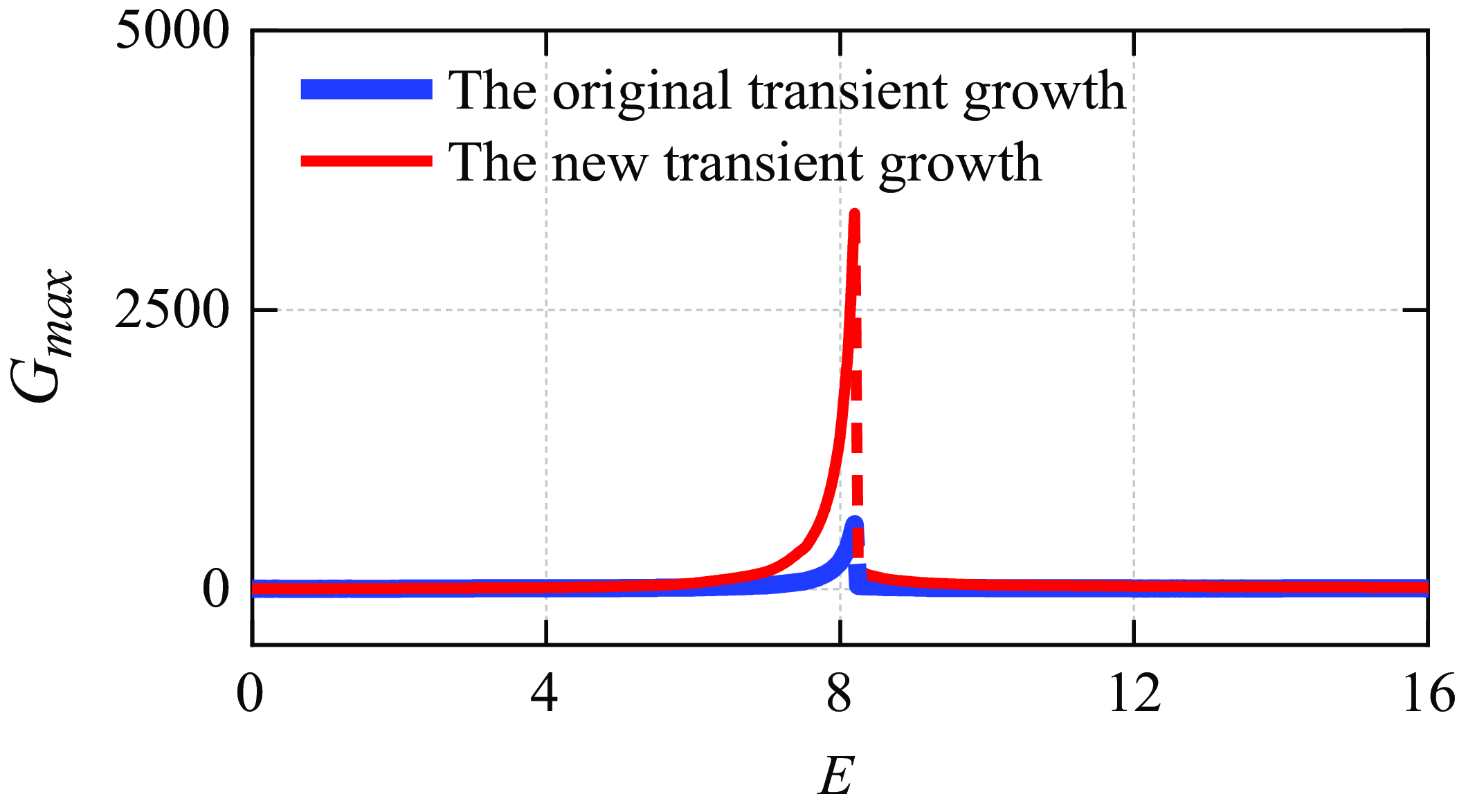
Since the initial transient growth here results from the viscoelasticity of fluids, one may expect a larger G max (the largest transient growth) at larger E. However, G max at E = 8.4 is in fact an order of magnitude lower than that at E = 8. It is interesting that the increase of elasticity cannot always lead to a larger value of G max , despite that the initial transient growth here benefits from the inclusion of viscoelasticity effects. This is an essential difference of present transient growth (which also includes thermal effects) from the one singly resulting from the viscoelasticity, i.e. the elastic growth in which transient growth of the streamwise component of the polymeric stresses tensor scales as W 2 (Jovanović & Kumar Reference Jovanović and Kumar2010), with W = ReE being the Weissenberg number. Specifically, from figure 5(a) which shows G max as a function of E, one sees that in stationary instability regime where E < E c , G max is an increasing function of E and particularly, near E = E c a very sharp increase is observed. In oscillatory instability regime where E > E c , however, after a sudden drop at E = E c , G max decreases slowly with increasing E and for sufficiently large E (e.g. E>20), the non-modal growth becomes negligible. Similar to G max , t max (the time to reach G max ) also undergoes a drastic change near E = E c (see figure 5 b). This means that in viscoelastic RB convection of finite E, the non-modal effects can sustain a long time to achieve significant transient growth only just before the Hopf bifurcation when the stationary instability transitions to the oscillatory instability; otherwise, the transient growth will be negligible. In order to explain this distinguishing phenomenon, we perform an input–output analysis to examine the influences of initial disturbance on the transient growth (corresponding to the input analysis) and to identify which energy component is most amplified in the optimal response (corresponding to the output analysis) and conduct an energy budget analysis within the interval of the transient amplification of disturbances.
The largest transient energy growth G max and the t max that attains G max as a function of E in marginally stable case, and the other parameters are β = 0.75, γ = 0, Pr = 10, Ra = Ra c and α = α c . Note that, for E < E c , Ra = 213.47 is used in (b) to ensure the accuracy of the calculation in t max .

The transient growth shown in figure 5 corresponds to cases where the fixed wavenumber equals the critical wavenumber. However, the wavenumber at which maximum transient energy growth is achieved does not coincide with this critical wavenumber, which is evidenced by figure 6(a). Specifically, in weakly elastic regime, α opt varies non-monotonically with increasing E and near the Hopf bifurcation α opt is the smallest and is close to α c , indicating that non-modal instability favours convection rolls of large cross-section like stationary convection instead of oscillatory convection. Since the non-modal growth is a result of interaction between various eigenmodes (including the least stable mode), α opt does not undergo a sudden jump like α c which only corresponds to the least stable mode, despite that it also increases rapidly near the Hopf bifurcation. On the other hand, different from the E dependence, Ra has rather small influence on α opt . As shown in figure 6(b), with the increase of Ra, the transient growth is significantly enhanced as expected, while α opt is only slightly decreased in both weakly and strongly elastic regimes.
(a) The optimal wavenumber α opt and the critical wavenumber α c as functions of E and (b) effects of Ra and α on G max at E = 8 and E = 8.4. Other parameters are β = 0.75, Pr = 10 and γ = 0.

In order to interpret how the transient growth due to viscoelasticity is achieved, we perform an input–output analysis. Firstly, inspecting the energy growth with different input filters displayed in figure 7(a,b), one observes that inputting different perturbations cannot change whether the instability is oscillatory or stationary, but changes the magnitude of transient energy amplification. Specifically, in both stationary and oscillatory instability regimes, the transient energy growth with only the temperature field perturbed initially (input temperature disturbance
 $\tilde{\theta }$
) is very close to the optimal transient growth over all possible initial conditions (input
 $\tilde{{v}}$
,
 $\tilde{\eta }$
,
 $\tilde{\theta }$
), while transient growth with other physical quantities perturbed initially is negligible. This dependence on initial disturbance is valid in both stationary and oscillatory instability regimes and it indicates that to induce this non-modal growth one needs to perturb the temperature field carefully with other physical fields remaining unperturbed. On the other hand, as shown in figure 7(c,d), it is noted that among various energy components, it is the thermal energy that is the most amplified, with
 $G_{o\_{{v}}}$
being moderately amplified and G
o_η
being always decayed. These two results highlight the significance of temperature disturbance and further confirm that the transient growth here is essentially different from the elastic growth (Jovanović & Kumar Reference Jovanović and Kumar2010) in which the elastic perturbation is dominant in both initial condition and optimal response. To reiterate, we omit elastic disturbance in the present study since we focus on the inertial case instead of the elastic case. Once the elastic disturbance is included the optimal response will be different. This case is illustrated in Appendix D. Specifically, as shown in figure 22, in this case, the elastic energy denoted by G
o_g
supersedes the thermal energy denoted by G
o_θ
to be the dominant disturbance energy in the optimal response, while the dependence on initial disturbances is only slightly changed.
Input–output analysis for (a) input analysis at E = 8, (b) input analysis at E = 8.4, (c) output analysis at E = 8, (d) output analysis at E = 8.4; and the other parameters are α = α c , γ = 0, Pr = 10 and β = 0.75.

Regarding the energy contribution during the transient growth, it is found that the energy coming from the base-state temperature gradient is the only source to drive the amplification of disturbances, which is evidenced by figure 8 (see Appendix B for detailed definitions and derivations of energy budget analysis). In contrast, the polymeric stresses appear to damp the non-modal instability, since PD is always negative. In fact, while the polymeric stresses do not contribute energy directly to the amplification of temperature perturbation
 $\tilde{\theta }$
, it promotes the energy transfer between temperature and wall-normal fluctuations; otherwise thermal effects itself cannot generate any transient growth, e.g. pure RB of Newtonian fluids.
Corresponding to figure 7, energy budget analysis for (a) E = 8; (b) E = 8.4 and (c) VT term and PD term in energy budget analysis as a function of E, where VT and PD are the maximum values on the corresponding energy budget analysis curves in (b) and these two notations have the same meaning in figure 12(b) and figure 22(c) later. Other parameters are the same as those in figure 7.

It is necessary to explain why energy production by the polymeric stresses does not account directly for the transient growth. The input–output analysis indicates that temperature disturbance is dominant in both initial conditions and in the optimal responses. From linearized equations (A1)–(A9), it is clear that there is no direct coupling between the temperature gradient and polymeric stresses. The indirect interaction between these two factors is attained by their individual interaction with the perturbed hydrodynamic field. Specifically,
 $\tilde{\theta }$
only directly interacts with
 $\tilde{{v}}$
while
 $\tilde{c}$
can directly interact with
 $\tilde{{v}}$
and
 $\tilde{\eta }$
. Therefore, here one cannot expect the potential energy due to the viscoelasticity to directly drive the amplification of disturbances in which the thermal energy is most amplified. On the other hand, from the input analysis shown in figure 7(a,b) one knows that the velocity fluctuations can hardly promote the transient growth. In this case, it is impossible for polymeric stresses to drive the movement of fluid parcel thus causing the significant transient growth shown in figures 5 and 7. This indirect effect of viscoelasticity to drive the transient growth of viscoelastic RB convection is similar to ‘catalysis’ and as shown in figure 8(c), this effect is most pronounced at E = E
c
, when the energy from the temperature gradient to the perturbed hydrodynamic field is the largest. After the Hopf bifurcation, the aforementioned energy transfer becomes ineffective and negligible. This explains the drastic change of G
max
shown in figure 5. It is worth noting that our results are highly consistent with Park & Lee (Reference Park and Lee1996) who showed that near E = E
c
the bifurcation is subcritical while the bifurcation is supercritical for E << E
c
or E >> E
c
. Finally, one notes in figure 8 that as expected, Prod is zero due to the absence of shear flow while VD is always negative since viscosity always damps the flow motion.
The drastic change of transient growth near the Hopf bifurcation is universal in viscoelastic RB convection, which is evidenced by examining a wide range of Pr and β. As shown in figure 9, when Pr varies from 0.01–100 and β from 0.05–0.9, the sharp increase before E = E c and sudden drop at E = E c of G max are always present. Specifically, it is seen that the transient growth of viscoelastic RB convection (as well as E c ) is larger at lower values of Pr or larger values of β. However, as shown in figure 9(c,d), different from the β dependence, t max varies non-monotonically with Pr, despite that G max is always a decreasing function of Pr.
Under marginally stable case, G max as a function of E for (a) different Pr; (b) different β and t max as a function of E for (c) different Pr and (d) different β. Other parameters are γ = 0, β = 0.75 in (a) and (c) and Pr = 10 in panels (b) and (d).

It is necessary to examine the shapes of inputs/outputs, which are shown in figure 10. It is seen from figure 10(a) that the contour of temperature perturbation
 $\tilde{\theta }$
is similar to that of the ordinary thermal instability, e.g. figure 1 of Shishkina (Reference Shishkina2021) and figure 12 of Hirata et al. (Reference Hirata, Alves, Delenda and Ouarzazi2015). During the evolution from the optimal initial condition to the optimal response, the shape of the perturbed temperature is almost unchanged (see figure 10
b), but its magnitude is significantly increased, which is evidenced by comparing the colourbar of figure 10(a,b) or by figure 10(c). The velocity vector resulting from the temperature gradient, denoted by black arrows in figure 10(a,b), consists of a pair of counter-rotating cells and is clearly intensified at the optimal response, which is consistent with the result of input–output analysis that
 $G_{o\_{{v}}}$
is moderately amplified during the non-modal growth. Regarding the six dependent components of the perturbed conformation tensor,
 $\tilde{{c}}$
13,
 $\tilde{{c}}$
23 and
 $\tilde{{c}}$
33 are always negligible during the transient growth so that they are not shown here. The non-negligible components, i.e.
 $\tilde{{c}}$
11,
 $\tilde{{c}}$
22 and
 $\tilde{{c}}$
12, have different distributions from
 $\tilde{\theta }$
. In contrast to tangential component
 $\tilde{{c}}$
12, as shown in figure 10(d), normal components
 $\tilde{{c}}$
11 and
 $\tilde{{c}}$
22, whose distributions are entirely identical, are maximal near y = ±0.5 and minimal at boundaries and centre of the domain. This property is due to the relationship between the perturbed conformation tensor and perturbed velocity field. Specifically, in this study, the polymeric stresses field is not perturbed initially, but perturbed indirectly by the velocity disturbances. Therefore, according to (A4), (A5) and (A7), it is expected that the distributions of
 $\tilde{{c}}$
11,
 $\tilde{{c}}$
22 and
 $\tilde{{c}}$
12 are analogous to ∂
 $\tilde{{u}}$
/∂x, ∂
 $\tilde{{v}}$
/∂y and ∂
 $\tilde{{u}}$
/∂y, respectively, see figure 10(d,e). This analogy is consistent with the numerical simulation of Zheng et al. (Reference Zheng, Hagani, Boutaous, Knikker, Xin and Siginer2022).
Cross-span view of perturbed velocity vectors and temperature perturbation for (a) optimal initial condition and (b) optimal response (note that the colourbar in (a) and (b) is used to illustrate temperature perturbation rather than velocity perturbation, and wavelength λ = 2π/α); (c) evolution of optimal initial temperature perturbation over time; (d) perturbed conformation tensor; (e) gradient of velocity perturbation at the time of optimal growth. Other parameters are the same as in figure 7(a).

4. Non-modal stability analysis of the RB–Poiseuille/Couette mixed convection
4.1. Low Re cases
In the presence of shear, it is fundamental to identify the orientation of disturbances that achieves the largest energy growth. To this end, figure 11 shows the contours of G max in the α–γ plane, from which it is seen that the presence of shear breaks the symmetry of G max with respect to α and γ. Specifically, regardless of whether it is Couette flow or Poiseuille flow imposed, streamwise-uniform disturbances always can achieve the largest energy amplification in both weakly and strongly elastic regimes, despite of different α dependence of G max in these two regimes. It should be noted that in the RB–Couette flow of Newtonian fluid, it is nearly longitudinal rolls that have the largest transient growth (Jerome et al. Reference Jerome, Chomaz and Huerre2012). The difference between our results and those of Jerome et al. (Reference Jerome, Chomaz and Huerre2012) is due to the existence of viscoelastic effects. It is well known that in RB–Couette/Poiseuille flow of Newtonian fluids, the mechanism of transient energy growth is identical to pure shear flows. Therefore, similar to the pure Couette flow, in RB–Couette flow of Newtonian fluid the nearly longitudinal rolls can achieve the largest transient growth due to the lift-up mechanism (Jerome et al. Reference Jerome, Chomaz and Huerre2012). However, RB in viscoelastic fluids can generate transient growth even in the absence of shear, as discussed in the last section. By comparing figure 11(a,d) and figure 11(b,c,e,f), it is found that the presence of a shear flow can inhibit the transient growth of viscoelastic RB convection with α> 0. In this case, longitudinal rolls can have the largest transient growth caused by the viscoelasticity effects. On the other hand, in pure Couette flow of both Newtonian fluids (Trefethen 1993; Schmid & Henningson Reference Schmid and Henningson2001) and viscoelastic fluids (Hoda et al. Reference Hoda, Jovanović and Kumar2008), nearly longitudinal rolls have the largest transient growth when α is close to zero. The superposition of transient growth by viscoelasticity and that by the lift-up mechanism makes longitudinal rolls instead of nearly longitudinal rolls have the largest transient growth in RB–Couette mixed flow of viscoelastic fluids.
Contours of G max in α-γ plane for (a) E = 4, hydrostatic state, (b) E = 4, Poiseuille flow, (c) E = 4, Couette flow, (d) E = 12, hydrostatic state, (e) E = 12, Poiseuille flow, (f) E = 12, Couette flow; and the other parameters are β = 0.75, Pr = 10, Re = 0.5 in (b), (c), (e) and (f), Ra = 213 for E = 4 and Ra = 196.846 for E = 12.

In viscoelastic RB–Couette flow, (a) the effect of Re on different transient growths, (b) VT term and PD term in energy budget analysis as functions of Re (note that VT rel = VT/(VT + PD) and PD rel = PD/(VT + PD)) and (c) the transition Reynolds number Re T as a function of E. Other parameters are β = 0.75, Pr = 10, α = 0, Ra = Ra c and γ = γ c .

In order to interpret how temperature gradient, viscoelasticity and shear affect the transient growth of viscoelastic RB-Couette flow, we perform an input–output analysis and transient energy analysis, see figure 12. Let us first have a look at the output. As shown in figure 12(a), there is a transition regarding G o_η . Specifically, once Re exceeds 1.986, G o_η will supersede G o_θ (which is always unchanged during the increase of Re) to be the dominant component of disturbance energy in the optimal response. As a result, the overall energy output G is increased with larger values of Re. It is interesting that in the presence of shear, the optimal initial condition is nearly unchanged, which is deduced by inspecting the curve marked by G i_θ shown in figure 12(a). Comparing G i_θ and G, it is found that the temperature disturbance is always dominant in the optimal initial condition regardless of the values of Re. This means that the imposing of shear into a viscoelastic RB convection does not affect how the non-modal growth should be triggered but significantly increases the magnitude of this non-modal growth. Figure 12(a) illustrates how this increase is achieved from the aspect of output energy, but the energy source to amplify disturbances is still unknown. Figure 12(b) gives the answer by showing the results of energy budget analysis. In order to highlight the transition, we only show VT and PD which are normalized as VT rel = VT/(VT + PD) and PD rel = PD/(VT + PD). It is surprising that near the transition it is PD instead of Prod (Prod is close to 0, not shown) that supersedes VT to be the dominant energy source of transient amplification. Apparently, Prod being nearly zero is because Re is too small here. In the high-Re regime examined in the next section, the energy production from the background shear is definitely non-negligible, see, for instance, figure 17. We postpone to the next section the explanation of how and why polymeric stresses can make considerable positive work to the amplification of disturbances even if they are not perturbed initially. Here, it is noted that the transition showing in figure 12(b) occurs at a lower Re than that in figure 12(a). This hysteresis is because G max is dependent on the integration of energy input (here it is VT and PD), rather than the energy input itself. Figure 17(a) is a perfect annotation of this hysteresis.
We use Re T at which G o_η exceeds G o_θ to denote the transition between different regimes. It is seen from figure 12(c) that this transitional Re, i.e. Re T , is a decreasing function of E. Specifically, there is no sudden jump of Re T at E c and after the Hopf bifurcation, Re T asymptotes to a constant.
Figure 13 illustrates the transient growth of the sheared viscoelastic RB with α = 0, which shares some analogies with the unsheared cases. As shown in figure 13(a), G evolves smoothly in stationary instability regime (E = 4) but periodically in oscillatory instability regime (E = 12), regardless it is Poiseuille flow or Couette flow imposed, and whether Re < Re T (i.e. Re = 0.5) or Re > Re T (i.e. Re = 10). On the other hand, as shown in figure 13(c), the transient growth is still maximized at E = E c . It is worth noting that while only shears of weak intensity are imposed, e.g. Re = 10, the transient growth at E = E c is surprisingly enhanced by at least an order of magnitude. For instance, at parameter settings considered in figure 13(c), G max = 580 in pure RB convection, G max = 4570 in RB-Poiseuille flow and G max = 12 750 in RB-Couette flow. It is clear that the transient growth here also benefits significantly from the viscoelastic effects and thermal effects, since the pure shear flows in this Re range cannot generate any transient growth, see figure 13(b). In addition, it is noted that different from the cases dominated by the viscoelastic effects at Re = 0.5, here t max at Re = 10 is not a decreasing function of E at E > E c . As shown in figure 13(d), for sufficiently large E, t max in fact increases with larger values of E, despite that this increase has no influence on the maximum energy gain in the optimal response, i.e. G max .
Figure 14 further studies the Re dependence of the transient growth of the viscoelastic mixed convection. As expected, in both cases of Poiseuille flow and Couette flow imposed, G max and t max are increasing functions of Re. Furthermore, it is surprising that except for the very small Re, i.e. the regime around Re = Re T , the scaling laws G max ∼Re 2 and t max ∼Re hold, which were originally found in pure bounded shear flows of high Re (Schmid & Henningson Reference Schmid and Henningson2001), are held here. Specifically, regarding the Re dependence of G max , the slope at oscillatory instability regime (E = 12) is much larger than that at E = 4 (stationary instability regime); note that G max at E = 4 is close to G max at E = 12 in the hydrostatic case. Regarding the Re dependence of t max , the slope is nearly independent of the type of shear flows and also independent of the elasticity, while t max is affected by the type of shear flow in purely bounded Newtonian shear flows (Schmid & Henningson Reference Schmid and Henningson2001). Therefore, t max here is only affected by the shear intensity, as shown in figure 14(c,d).
Transient energy growth G of streamwise-uniform disturbances for (a) Ra = 213 (for E = 4), Ra = 196 (for E = 12) and (b) Ra = 0; effects of elasticity number E on (c) G max and (d) t max . Other parameters are α = 0, β = 0.75, Ra = Ra c (for panels (c, d)), γ = γ c , Pr = 10 and Re = 0.5, 10. Note that, for E < E c , ra = 213 is used in (d) to ensure the accuracy of t max .

Effects of Re on (a) G max , E = 4, (b) G max , E = 12, (c) t max , E = 4, (d) t max , E = 12; and the other parameters are α = 0, β = 0.75, Ra = Ra c , γ = γ c and Pr = 10.

One remaining notable phenomenon here concerns the differences between the Poiseuille flow and Couette flow. As shown in figure 14(a,b), whether it is a strongly elastic fluid or a weakly elastic fluid, G
max
in viscoelastic RB-Couette flow is always greater than that in viscoelastic RB-Poiseuille flow, and this difference becomes more significant as Re increases. Similar results can be found in the plane Poiseuille/Couette flow of viscoelastic fluids studied by Hoda et al. (Reference Hoda, Jovanović and Kumar2008) who assumed that this difference may depend on the correlation between the vortex stretching term and vertical scale y. Specifically, for Newtonian plane Poiseuille/Couette flow, it has been proved that the vortex stretching term is proportional to
 $\overline{U}^{\prime}\partial _{z}{v}$
, so the vortex stretching term depends linearly on y in Poiseuille flow, i.e.
 $\overline{U}^{\prime}=-2y$
and it is independent of y in Couette flow, i.e.
 $\overline{U}^{\prime}=1$
(Landahl Reference Landahl1975; Butler & Farrell Reference Butler and Farrell1992; Hoda et al. Reference Hoda, Jovanović and Kumar2008). Due to the strongly non-trivial coupling between thermal-hydrodynamic equations and polymer molecular constitutive equations, the exact reasons of aforementioned difference between viscoelastic RB–Couette flow and viscoelastic RB-Poiseuille flow cannot be determined at present, but the phenomenon in figure 14(a,b) is indeed consistent with those results of pure shear flows (Landahl Reference Landahl1975; Butler & Farrell Reference Butler and Farrell1992; Hoda et al. Reference Hoda, Jovanović and Kumar2008).
Effects of Ra and E on transient energy growth of Couette flow for (a) viscoelastic fluid at Ra = 0, (b) Newtonian fluid and (c) viscoelastic fluid at Ra = 100, (d) viscoelastic fluid at E = 12 and (e) effects of β on transient growth at Ra = 213 and E = 1. Other parameters for are Re = 2000, β = 0.75, Pr = 10, α = 0, γ = γ c .

4.2. High Re cases
Now we turn to investigate the transient energy growth of mixed convection at relatively high Re, i.e. Re∼O(103). It should be noted that the Poiseuille flow can be linearly unstable to the Tollmien–Schlichting waves at Re = 5772.22 (Orszag Reference Orszag1971) for Newtonian fluid and particularly, to a newly found instability, i.e. the centre mode (Khalid et al. Reference Khalid, Chaudhary, Garg, Shankar and Subramanian2021), at much lower Re for viscoelastic fluid. Therefore, to highlight the non-modal instability of the sheared RB convection of viscoelastic fluids in high-Re regime, we only consider the case of Couette flow imposed, which, in both Newtonian (Schmid & Henningson Reference Schmid and Henningson2001) and viscoelastic fluids (Chaudhary et al. Reference Chaudhary, Garg, Shankar and Subramanian2019), is always linearly stable.
In the case of high Re, pure shear flow can cause a large transient energy growth in both Newtonian (Schmid & Henningson Reference Schmid and Henningson2001; Schmid Reference Schmid2007) and viscoelastic fluids (Hoda et al. Reference Hoda, Jovanović and Kumar2008; Zhang et al. Reference Zhang, Lashgari, Zaki and Brandt2013). In figure 15 we show how the viscoelasticity and temperature gradient affect the transient growth by the lift-up mechanism. Specifically, as shown in figure 15(a), viscoelasticity has an enhancing effect on the transient growth by the lift-up mechanism and with the increase of the elasticity, this enhancement is more significant. Similarly, an unstable temperature gradient can also enhance the transient growth by the lift-up mechanism, as shown in figure 15(b). The difference between these two cases lies in that viscoelasticity can significantly increase G max with t max being nearly unchanged, while heat can significantly extend t max and cause the generation of the second peak which is higher than the first one for large Ra, see figure 15(b). This implies that the ways of viscoelasticity and heat to enhance the transient growth of high-Re shear flow are different. This point will be clarified later. As shown in figure 15(c,d), once the viscoelasticity and an unstable temperature gradient are simultaneously included, the second peak of the G(t) curve will be further increased and the disturbance energy will be most amplified in this peak instead of in the first peak. In this case, G max is always an increasing function of both E and Ra, which is different from the non-monotonic variation of G max with E in figure 5. It should be noted that for a concentrated solution, e.g. β = 0.15, the first peak is always the largest (see figure 15 e), indicating that the significant enhancement of the second peak is only effective for a dilute solution.
(a) Input analysis and (b) output analysis at E = 12 and ra = 100, and the other parameters are the same as in figure 15(c).

Transient energy analysis at high Re = 2000 for (a) pure Couette flow of Newtonian fluid, (b) RB–Couette flow of Newtonian fluid, (c) pure Couette flow of viscoelastic fluid and (d) RB–Couette flow of viscoelastic fluid. Other parameters are β = 1 (panel (a)) or 0.75 (panels (b), (c) and (d)), E = 12, Pr = 10, α = 0 and γ = γ c = 1.558 (Newtonian) or 1.66 (viscoelastic).

Here we are interested in the case of dilute solution where the enhancement due to viscoelasticity and heat is related to the generation for the second peak of the G(t) curve. Figures 16 and 17 give an insight into the second peak. From the input analysis shown in figure 16(a), one sees that when wall-normal velocity
 ${v}$
is perturbed initially, the disturbance energy will be maximized in the first peak, while the disturbance energy will be maximized in the second peak when only temperature is perturbed initially, which indicates the dependence of these two peaks of G(t) on different input disturbances, i.e. the non-normality of the linear operator forming the first peak is mainly related to the hydrodynamics, while the non-normality of the linear operator forming the second peak is mainly related to the perturbed temperature field. Regarding the output analysis shown in figure 16(b), it is seen that, the main energy output of these two peaks is the kinetic energy of perturbed wall-normal vorticity (similar to the transient growth of pure Couette flow) while the thermal energy output is very small. Therefore, the shape of the optimal initial condition here is identical to the unsheared viscoelastic RB convection while in the optimal response, one expects the formation of streamwise streaks as with the pure Couette flow, which is evidenced by figure 18(a,b,c).
(a) Cross-stream view of perturbed velocity vectors and temperature perturbation of the optimal initial condition (note that this colourbar is used to illustrate temperature perturbation rather than velocity perturbation, and wavelength λ = 2π/γ); (b) cross-stream view of perturbed streamwise velocity
 $\tilde{{u}}$
at the first peak (above) / the second peak (i.e. optimal response, below); (c) perturbed velocity of optimal response; (d) perturbed conformation tensor at the time of optimal growth and (e) PD components in transient energy analysis. Other parameters are the same as those in figure 17(d).

In the transient energy analysis shown in figure 17, we compare the short-term energy budget of four typical cases aforementioned, i.e. the pure Couette flow of Newtonian fluid shown in figure 17(a), the RB–Couette flow of Newtonian fluid shown in figure 17(b), the pure Couette flow of viscoelastic fluid shown in figure 17(c) and the RB–Couette flow of viscoelastic fluid shown in figure 17(d). As expected, in the first case, the energy from the mean shear is the only energy source to amplify the disturbance and the viscous dissipation is the only energy loss to damp the non-modal instability. Interestingly, it is found that in the second case shown in figure 17(b) the presence of an unstable temperature gradient does not change the dominant energy balance mentioned above, especially VT ≈ 0. However, the presence of the temperature gradient promotes the mean shear to release more energy into the perturbed hydrodynamic field, which is evidenced by the slower decay of Prod in figure 17(b) compared with that in figure 17(a). This result is consistent with the previous idea that the temperature gradient can enhance the classical lift-up mechanism by extending its duration (Jerome et al. Reference Jerome, Chomaz and Huerre2012). Consequently, the action of an unstable temperature gradient results in the second growth (peak) of the disturbance energy, as shown in figure 17(b). The case of the pure Couette flow of viscoelastic fluid shown in figure 17(c) is similar to that of Newtonian fluid shown in figure 17(a), with the presence of polymeric stresses favouring the energy production by the base flow. This point has been well understood in previous studies, e.g. Zhang et al. (Reference Zhang, Lashgari, Zaki and Brandt2013). When polymeric stresses and temperature gradient are simultaneously included, one expects an interesting energy balance shown in figure 17(d). As expected, the amplification of disturbances corresponding to the first peak of G(t) curve results from the energy production by the basis shear. Different from the temperature field whose energy contribution is always negligible as before, here polymeric stresses field can absorb non-negligible energy from the perturbed hydrodynamic field. However, it is surprising that as the second peak is achieved, PD becomes the dominant energy source while at the same time, Prod becomes negligible. This result is rather counterintuitive since the polymeric stresses field is not perturbed initially, i.e., it is impossible for polymeric stresses field to store any energy initially. Therefore, it is necessary to figure out how the disturbance energy is transferred into the polymeric stresses field and then into the perturbed hydrodynamic field. We have known from figure 8 that polymeric stresses field can absorb disturbance energy from the temperature field. Since the temperature field and the polymeric stresses field are not coupled directly, temperature field cannot transfer energy to polymeric stresses field directly. As mentioned before, this energy transfer includes two processes: (i) the energy transfer from temperature field to hydrodynamic field and (ii) energy transfer from hydrodynamic field to polymeric stresses field. Physically, temperature disturbance perturbs the hydrodynamic field, which in turn perturbs the polymeric stresses field. On the other hand, polymeric stresses field can also obtain energy from the base flow when a background shear is present. Specifically, as pointed out by Buza, Page & Kerswell (Reference Buza, Page and Kerswell2022), the polymer energy has four sources, i.e. the energies from the base flow, the perturbed hydrodynamic field (here, to reiterate, this kind of energy partially or mainly results from the temperature field), the polymeric relaxation and polymeric diffusion, see (4.8) in Buza et al. (Reference Buza, Page and Kerswell2022). In the present system, after the energy from the base flow and from the temperature gradient enters the polymeric stresses field, it is partially transferred into the perturbed hydrodynamic field (the remaining part causes the amplification of elastic energy, see figure 18
d), thus driving the amplification of the perturbed wall-normal vorticity. This process is essentially different from the classical lift-up mechanism. Specifically, as shown in figure 18(e), among various components in PD,
 $\tilde{{c}}$
12 and
 $\tilde{{c}}$
13 have significant influence on the energy transfer between the perturbed polymeric stresses field and velocity fluctuation field. Here
 $\tilde{{c}}$
12 causes the energy transfer from the perturbed polymeric stresses field to velocity fluctuation field, which exceeds the opposite energy transfer caused by
 $\tilde{{c}}$
13. Therefore, one expects large, positive values of PD in energy budget analysis shown in figure 17(d). Our results are consistent with Hoda et al. (Reference Hoda, Jovanović and Kumar2008, Reference Hoda, Jovanović and Kumar2009) who also found that
 $\tilde{{c}}$
12 and
 $\tilde{{c}}$
13 can enhance and suppress transient growth of velocity disturbances in channel flows with very high fluid elasticity, respectively.
5. Conclusion
In this paper, we study the non-modal instability of RB convection with and without wall bounded shear flows in Oldroyd-B fluid.
In the absence of shear flow, viscoelasticity causes transient energy growth of RB convection, in which the perturbed thermal energy grows the most. During the bifurcation from stationary instability dominated by fluid viscosity to oscillatory instability dominated by fluid elasticity, both the maximum growth G max and the time to attain G max , i.e. t max , reach their maximums. This is because at this Hopf bifurcation, the system allows more energies transferred from the temperature field into the perturbed hydrodynamic field to drive the vertical movement of fluid particle. Increasing viscosity ratio β and decreasing Prandtl number Pr can significantly increase the maximum G max , which can reach 104.
In the presence of Poiseuille/Couette flow, streamwise-uniform perturbations can achieve the largest energy amplification in both weakly and strongly elastic regimes. The transient growth at very low Reynolds number Re is similar to the unsheared case. With the increase of Re, however, a transition arises and the classical scaling: G max ∝ Re 2 and t max ∝ Re hold. At high-Re cases, there are two peaks of transient energy growth, in which the kinetic energy of perturbed wall-normal vorticity is the most amplified. The first peak only depends on Re, while the second peak is simultaneously determined by temperature gradient, elasticity and shear intensity. With an increase in Rayleigh number Ra and elasticity number E, the maximum energy growth transitions from the first peak to the second peak. At the second peak, the energy production from the temperature field and background flow is indirectly transferred into the perturbed wall-normal vorticity under the action of polymeric stresses.
Our results may provide a new perspective for understanding and controlling the early transition to the elastoinertial turbulence under the action of an unstable temperature gradient.
Acknowledgements
This work is supported by the National Natural Science Foundation of China (grants no. 52276057 and no. 52076055) and the Postdoctoral Science Foundation of Heilongjiang Province (grant no. LBH-TZ2209). We also acknowledge the MOE grant A- 8001172-00-00.
Declaration of interests
The authors report no conflict of interest.
Appendix A. Perturbation equations
In this appendix, we provide the complete linear perturbation equations as follows:
 \begin{align} \left(\frac{\partial ^{2}}{\partial y^{2}}-k^{2}\right)\frac{\partial }{\partial t}\tilde{{v}} & = \left[-i\alpha \overline{U}\cdot \left(\frac{\partial ^{2}}{\partial y^{2}}-k^{2}\right)+i\alpha \overline{U}^{\prime\prime}+\frac{\beta }{Re}\left(\frac{\partial ^{2}}{\partial y^{2}}-k^{2}\right)^{2}\right]\tilde{{v}} \notag\\ & \quad + \frac{Ra}{Re^{2}Pr} \left(\nabla^{2} - \dfrac{\partial^{2}}{\partial y^{2}} \right) \tilde{\theta} \notag\\ & \quad +\frac{1-\beta }{Re^{2}E}\left(\!\!\!\begin{array}{c} \alpha ^{2}\dfrac{\partial \tilde{c}_{11}}{\partial y}-k^{2}\dfrac{\partial \tilde{c}_{22}}{\partial y}+\gamma ^{2}\dfrac{\partial \tilde{c}_{33}}{\partial y}\\ -i\alpha\! \left(\dfrac{\partial ^{2}}{\partial y^{2}}+k^{2}\right)\tilde{c}_{12}+2\alpha \gamma \dfrac{\partial \tilde{c}_{13}}{\partial y}-i\gamma \!\left(\dfrac{\partial ^{2}}{\partial y^{2}}+k^{2}\right)\tilde{c}_{23} \end{array}\!\!\!\right)\!,\end{align}
 \begin{align} \frac{\partial }{\partial t}\tilde{\eta } & =-i\gamma \overline{U}^{\prime}\tilde{{v}}+\left(\frac{\beta }{Re}\left(\frac{\partial ^{2}}{\partial y^{2}}-k^{2}\right)-i\alpha \overline{U}\right)\tilde{\eta }\nonumber\\&\quad +\frac{1-\beta }{Re^{2}E}\left(-\alpha \gamma \tilde{c}_{11}+\alpha \gamma \tilde{c}_{33}+i\gamma \frac{\partial \tilde{c}_{12}}{\partial y}+\left(\alpha ^{2}-\gamma ^{2}\right)\tilde{c}_{13}-i\alpha \frac{\partial \tilde{c}_{23}}{\partial y}\right), \end{align}
 \begin{equation} \frac{\partial }{\partial t}\tilde{\theta }=-\overline{\Theta}^{\prime}\tilde{{v}}+\left(-i\alpha \overline{U}+\frac{1}{RePr}\left(\frac{\partial ^{2}}{\partial y^{2}}-k^{2}\right)\right)\tilde{\theta }, \end{equation}
 \begin{align} \frac{\partial }{\partial t}\tilde{c}_{11}& =\frac{1}{k^{2}}\left(2\left(-\alpha ^{2}\overline{C}_{11}\frac{\partial }{\partial y}+i\alpha \overline{C}_{12}\frac{\partial ^{2}}{\partial y^{2}}\right)-k^{2}\overline{C}^{\prime}_{11}\right)\tilde{{v}} +\frac{2}{k^{2}}\left(\alpha \gamma \overline{C}_{11}-i\gamma \overline{C}_{12}\frac{\partial }{\partial y}\right)\tilde{\eta }\notag\\ & \quad -\left(i\alpha \overline{U}+\frac{1}{ReE}\right)\tilde{c}_{11}+2\overline{U}^{\prime}\tilde{c}_{12}\,, \end{align}
 \begin{equation} \frac{\partial }{\partial t}\tilde{c}_{22}=\left(2\left(i\alpha \overline{C}_{12}+\overline{C}_{22}\frac{\partial }{\partial y}\right)-\overline{C}^{\prime}_{22}\right)\tilde{{v}}-\left(i\alpha \overline{U}+\frac{1}{ReE}\right)\tilde{c}_{22}\,, \end{equation}
 \begin{equation} \frac{\partial }{\partial t}\tilde{c}_{33}=\frac{1}{k^{2}}\left(-2\gamma ^{2}\overline{C}_{33}\frac{\partial }{\partial y}-k^{2}\overline{C}^{\prime}_{33}\right)\tilde{{v}}-\frac{1}{k^{2}}\left(2\alpha \gamma \overline{C}_{33}\right)\tilde{\eta }-\left(i\alpha \overline{U}+\frac{1}{ReE}\right)\tilde{c}_{33}\,, \end{equation}
 \begin{align} \frac{\partial }{\partial t}\tilde{c}_{12}& =\frac{1}{k^{2}}\left(k^{2}\left(i\alpha \overline{C}_{11}+\overline{C}_{12}\frac{\partial }{\partial y}\right)-k^{2}\overline{C}^{\prime}_{12}+i\alpha \overline{C}_{22}\frac{\partial ^{2}}{\partial y^{2}}-\alpha ^{2}\overline{C}_{12}\frac{\partial }{\partial y}\right)\tilde{{v}}\notag\\[5pt] & \quad +\frac{1}{k^{2}}\left(\alpha \gamma \overline{C}_{12}-i\gamma \overline{C}_{22}\frac{\partial }{\partial y}\right)\tilde{\eta } +\overline{U}^{\prime}\tilde{c}_{22}-\left(i\alpha \overline{U}+\frac{1}{ReE}\right)\tilde{c}_{12}, \end{align}
 \begin{align} \frac{\partial }{\partial t}\tilde{c}_{13} & =\frac{1}{k^{2}}\left(-\alpha \gamma \overline{C}_{11}\frac{\partial }{\partial y}+i\gamma \overline{C}_{12}\frac{\partial ^{2}}{\partial y^{2}}-\alpha \gamma \overline{C}_{33}\frac{\partial }{\partial y}\right)\tilde{{v}}\nonumber\\& \quad +\frac{1}{k^{2}}\left(-\alpha ^{2}\overline{C}_{11}+i\alpha \overline{C}_{12}\frac{\partial }{\partial y}+\gamma ^{2}\overline{C}_{33}\right)\tilde{\eta } -\left(i\alpha \overline{U}+\frac{1}{ReE}\right)\tilde{c}_{13}+\overline{U}^{\prime}\tilde{c}_{23}\,, \end{align}
 \begin{align} \frac{\partial }{\partial t}\tilde{c}_{23} & =\frac{1}{k^{2}}\left(i\gamma \overline{C}_{22}\frac{\partial ^{2}}{\partial y^{2}}-\alpha \gamma \overline{C}_{12}\frac{\partial }{\partial y}+ik^{2}\gamma \overline{C}_{33}\right)\tilde{{v}} +\frac{1}{k^{2}}\left(-\alpha ^{2}\overline{C}_{12}+i\alpha \overline{C}_{22}\frac{\partial }{\partial y}\right)\tilde{\eta }\nonumber\\[5pt]& \quad -\left(i\alpha \overline{U}+\frac{1}{ReE}\right)\tilde{c}_{23}\, \end{align}
where boundary conditions are
 \begin{equation} \tilde{{v}}\left(\pm 1,t\right)=0, \tilde{{v}}^{\prime}\left(\pm 1,t\right)=0, \tilde{\eta }\left(\pm 1,t\right)=0, \tilde{\theta }\left(\pm 1,t\right)=0. \end{equation}
The perturbation boundary conditions of the conformation tensor
 $\tilde{\boldsymbol{c}}$
are not required since there are no terms involving derivatives of these stresses with respect to y (Zhang et al. Reference Zhang, Lashgari, Zaki and Brandt2013).
Appendix B. Transient energy analysis
To explain the instability mechanism, we introduce an energy budget analysis. The hydrodynamic perturbation kinetic energy is obtained by multiplying (2.8b
) by the complex conjugate velocity
 $u_{i}^{\dagger }$
:
 \begin{equation} u_{i}^{\dagger }\frac{\partial u_{i}}{\partial t}\!=\!-u_{i}^{\dagger }u_{j}\frac{\partial \overline{U}_{i}}{\partial x_{j}}\!-\!u_{i}^{\dagger }\overline{U}_{j}\frac{\partial u_{i}}{\partial x_{j}}-u_{i}^{\dagger }\frac{\partial p}{\partial x_{i}}\!+\!u_{i}^{\dagger }\frac{\beta }{Re}\frac{\partial ^{2}u_{i}}{\partial {x_{j}}^{2}}+u_{i}^{\dagger }\frac{1-\beta }{Re^{2}E}\frac{\partial c_{ij}}{\partial x_{j}}+\frac{Ra}{Re^{2}Pr}u_{i}^{\dagger }\theta \mathbf{1}_{\boldsymbol{y}} . \end{equation}
Then, taking the complex conjugate of (B1) to obtain a new equation, and averaging these two equations, which leaves us with
 \begin{align} \frac{\partial \varepsilon }{\partial t} & =-\frac{\beta }{Re}\frac{\partial u_{i}^{\dagger }}{\partial x_{j}}\frac{\partial u_{i}}{\partial x_{j}}-\frac{1-\beta }{2Re^{2}E}\left(c_{ij}\frac{\partial u_{i}^{\dagger }}{\partial x_{j}}+c_{ij}^{\dagger }\frac{\partial u_{i}}{\partial x_{j}}\right)-\frac{1}{2}\left(u_{i}^{\dagger }u_{j}\frac{\partial \overline{U}_{i}}{\partial x_{j}}+u_{i}u_{j}^{\dagger }\frac{\partial \overline{U}_{i}}{\partial x_{j}}\right)\nonumber\\[5pt] & \quad +\frac{1}{2}\frac{Ra}{Re^{2}\cdot Pr}\left(\theta u_{i}^{\dagger }+\theta ^{\dagger }u_{i}\right)\mathbf{1}_{y}\nonumber\\& \quad +\frac{\partial }{\partial x_{j}}\left[\!\!\begin{array}{c} -\dfrac{1}{2}u_{i}u_{i}^{\dagger }\overline{U}_{j}-\dfrac{1}{2}\left(u_{i}p^{\dagger }+u_{i}^{\dagger }p\right)\delta _{ij}\\[6pt] +\dfrac{\beta }{2Re}\left(u_{i}^{\dagger }\dfrac{\partial u_{i}}{\partial x_{j}}+u_{i}\dfrac{\partial u_{i}^{\dagger }}{\partial x_{j}}\right)+\frac{1-\beta }{2Re^{2}E}\left(u_{i}^{\dagger }c_{ij}+u_{i}c_{ij}^{\dagger }\right) \end{array}\!\!\!\!\right], \end{align}
where
 $\varepsilon = {u_{i}^{\dagger } u_{i}}/{2}$
is the perturbation energy density. In addition, in the case of periodic boundary conditions in the x and z directions as well as no-penetration and no-slip boundary conditions in the y direction, the transport terms in the square brackets have no effect on the energy balance.
For the transient energy analysis of non-modal analysis, the initial condition is the optimal initial condition. According to the definition of Butler & Farrell (Reference Butler and Farrell1992) and Zhang et al. (Reference Zhang, Lashgari, Zaki and Brandt2013, Reference Zhang, Martinelli, Wu, Schmid and Quadrio2015), we integrate and average (B2) on the control volume
 $\unicode{x1D6FA}$
,
 \begin{align} \frac{1}{\Omega }\int _{\Omega }\frac{\partial \varepsilon }{\partial t}{\mathrm{d}}V & =\frac{1}{\Omega }\int _{-1}^{1}\int _{0}^{a}\int _{0}^{b}\frac{\partial }{\partial t}\left(\frac{u^{2}+{v}^{2}+w^{2}}{2}\right){\mathrm{d}}V\nonumber\\[5pt] & =\frac{1}{\Omega }\int _{-1}^{1}\int _{0}^{a}\int _{0}^{b}\left[\underset{Prod}{\underbrace{-uv\frac{\mathrm{d}\overline{U}}{\mathrm{d}y}}}\underset{VD}{\underbrace{-\frac{\beta }{Re}\frac{\partial u_{i}}{\partial x_{j}}\frac{\partial u_{i}}{\partial x_{j}}}}\underset{PD}{\underbrace{-\frac{1-\beta }{Re^{2}E}c_{ij}\frac{\partial u_{i}}{\partial x_{j}}}}\right.\nonumber\\& \quad \left. \underset{VT}{\underbrace{+\frac{Ra}{Re^{2}Pr}\theta {v}}}\right]{{\mathrm{d}}z{\mathrm{d}}x{\mathrm{d}}y}\,, \end{align}
where the first term (Prod) on the right-hand side represents the energy production from mean shear flow, the second term (VD) indicates viscous dissipation whose value always remains negative, the third term (PD) describes the work rate of the polymeric stresses which can also represent the energy transfer between the perturbation velocity field and the perturbation polymeric stresses field in other words, the final term (VT) represents the work rate of the buoyancy force and also means the energy exchanged in the interaction between the perturbation velocity field and the perturbation temperature field. Moreover, if the values of some terms are positive, it means that these terms contribute to an increase in the perturbation kinetic energy, enhancing instability and vice versa. In addition, variables
 $\unicode{x1D6FA}$
, a and b are defined in § 2.4.
Appendix C. Numerical methods and code validation
In order to discretize and solve the eigenvalue problem (2.12) and the transient energy amplification (2.18), the spectral collocation method based on Chebyshev modes is used and its related differential and integral matrices can be found in Trefethen (Reference Trefethen2000), Weideman & Reddy (Reference Weideman and Reddy2000) and Canuto et al. (Reference Canuto, Hussaini, Quarteroni and Zang2007).
The validation of our stability code includes two parts. In the first part, we calculate the least stable mode of viscoelastic plane Poiseuille flow and the linear onset of RB–Poiseuille/Couette mixed flow in viscoelastic fluids. As shown in table 3, good agreement between our results and those of Zhang et al. (Reference Zhang, Lashgari, Zaki and Brandt2013) and Khalid et al. (Reference Khalid, Chaudhary, Garg, Shankar and Subramanian2021) is achieved when Chebyshev points N = 250 are used. In addition, due to the presence of the continuous spectrum (Khalid et al. Reference Khalid, Chaudhary, Garg, Shankar and Subramanian2021), more Chebyshev points are required when the value of E is very large. Regarding the critical Rayleigh number Ra c and the critical streamwise wavenumber α c , it is seen from figure 19 that our results are in good agreement with the results of Hirata et al. (Reference Hirata, Alves, Delenda and Ouarzazi2015) and Alves et al. (Reference Alves, Hirata and Ouarzazi2016). Besides, since half of the upper and lower plate spacing is used as the dimensionless length scale, it is worth noting that, Ra c and α c in the present results are 1/8 and 1/2 of the results of Chandrasekhar (Reference Chandrasekhar1961), Hirata et al. (Reference Hirata, Alves, Delenda and Ouarzazi2015) and Alves et al. (Reference Alves, Hirata and Ouarzazi2016), respectively.
Comparison and validation of our present results with the results of Zhang et al. (Reference Zhang, Lashgari, Zaki and Brandt2013) at Re = 3960, β = 0.5, E = 0.001, α = 1.15, γ = 0, Ra = 0 and Pr = 10, and Khalid et al. (Reference Khalid, Chaudhary, Garg, Shankar and Subramanian2021) at Re = 1990, β = 0, E = 0.003, α = 1.2, γ = 0, Ra = 0 and Pr = 10.

Validation of Ra c (a–d) and α c (e–h) with the results of Hirata et al. (Reference Hirata, Alves, Delenda and Ouarzazi2015) and Alves et al. (Reference Alves, Hirata and Ouarzazi2016) in modal analysis. Other parameters are β = 0.75, γ = 0 and Pr = 10.

In the second part, we calculate the maximum growth G max and the time evolution of energy budget. As shown in figure 20, using 250 Chebyshev points, our results are in good agreement with the results of Zhang et al. (Reference Zhang, Lashgari, Zaki and Brandt2013).
Appendix D. Supplementary results with elastic disturbances and elastic potential energy
Here, we discuss a non-modal transient growth when the polymer is perturbed directly and the elastic potential energy is defined.
For the measure of elastic energy, we refer to the new definition introduced by Hameduddin et al. (Reference Hameduddin, Meneveau, Zaki and Gayme2018, Reference Hameduddin, Gayme and Zaki2019) instead of the traditional definition (Doering, Eckhardt & Schumacher Reference Doering, Eckhardt and Schumacher2006; Comminal, Spangenberg & Hattel Reference Comminal, Spangenberg and Hattel2015). The geometric decomposition of polymer tensor,
 $\boldsymbol{G}=\overline{\boldsymbol{G}}+\boldsymbol{g}$
is used instead of the classical Reynolds decomposition
 $\boldsymbol{C}=\overline{\boldsymbol{C}}+\boldsymbol{c}$
, where the base state
 $\overline{\boldsymbol{G}}=\boldsymbol{I}$
. Applying a Cholesky decomposition to the base conformation tensor
 $\overline{\boldsymbol{C}}=\boldsymbol{HH}^{\dagger }$
, the conversion between the perturbation conformation tensor c and g is
 \begin{equation} \boldsymbol{c}=\boldsymbol{C}-\overline{\boldsymbol{C}}=\boldsymbol{H}\cdot \boldsymbol{G}\cdot \boldsymbol{H}^{\dagger }-\boldsymbol{H}\cdot \overline{\boldsymbol{G}}\cdot \boldsymbol{H}^{\dagger }=\boldsymbol{H}\cdot \left(\boldsymbol{G}-\overline{\boldsymbol{G}}\right)\cdot \boldsymbol{H}^{\dagger }=\boldsymbol{H}\cdot \boldsymbol{g}\cdot \boldsymbol{H}^{\dagger }\, .\end{equation}
Therefore, the explicit expression of g = Pc can be written as
 \begin{equation} \left(\begin{array}{l} g_{11}\\ g_{22}\\ g_{33}\\ g_{12}\\ g_{13}\\ g_{23} \end{array}\right)=\left(\begin{array}{cccccc} \frac{\overline{C}_{22}}{\overline{S}^{2}} & \frac{1}{\overline{S}^{2}}\frac{\overline{C}_{12}^{2}}{\overline{C}_{22}} & 0 & -\frac{2\overline{C}_{12}}{\overline{S}^{2}} & 0 & 0\\[8pt] 0 & \frac{1}{\overline{C}_{22}} & 0 & 0 & 0 & 0\\[8pt] 0 & 0 & \frac{1}{\overline{C}_{33}} & 0 & 0 & 0\\[8pt] 0 & -\frac{\overline{C}_{12}}{\overline{C}_{22}\overline{S}} & 0 & \frac{1}{\overline{S}} & 0 & 0\\[8pt] 0 & 0 & 0 & 0 & \frac{\sqrt{\overline{C}_{22}}}{\overline{S}\sqrt{\overline{C}_{33}}} & -\frac{\overline{C}_{12}}{S\sqrt{\overline{C}_{22}\overline{C}_{33}}}\\[11pt] 0 & 0 & 0 & 0 & 0 & \frac{1}{\sqrt{\overline{C}_{22}\overline{C}_{33}}} \end{array}\right)\left(\begin{array}{l} c_{11}\\ c_{22}\\ c_{33}\\ c_{12}\\ c_{13}\\ c_{23} \end{array}\right), \end{equation}
where
 $\overline{S}=\sqrt{\overline{C}_{22}\overline{C}_{11}-\overline{C}_{12}^{2}}$
.
Validation of the largest transient energy amplification G max and transient energy evolution with those of Zhang et al. (Reference Zhang, Lashgari, Zaki and Brandt2013) in non-modal analysis. The parameters are (a) Re = 6000, β = 1, E = 1, α = 0, Ra = 0 and Pr = 10; (b) Re = 2000, β = 0.5, E = 0.006, α = 0, γ = 2, Ra = 0 and Pr = 10; (c) Re = 2000, β = 0.5, E = 0.006, α = 2, γ = 2, Ra = 0 and Pr = 10.

In this case, the revised energy norm is defined as
 \begin{align} \int _{{\Omega} }\varepsilon {\mathrm{d}}V & =\int _{{\Omega} }\left(\varepsilon _{k}+\varepsilon _{T}+\varepsilon _{c}\right)\mathrm{d}V\nonumber\\ & =\frac{1}{2}\times \frac{1}{2}\int _{{\Omega} }\left(\left(\left| \tilde{u}\right| ^{2}+\left| \tilde{{v}}\right| ^{2}+\left| \tilde{w}\right| ^{2}\right)+\frac{Ra}{Re^{2}Pr}| \tilde{\theta }| ^{2}+\frac{1-\beta }{Re^{2}E}tr(\tilde{\boldsymbol{g}}^{2})\right)\mathrm{d}V\nonumber\\ &=\int _{{\Omega} }\tilde{\boldsymbol{\chi }}^{\dagger }\boldsymbol{M}\tilde{\boldsymbol{\chi }}\mathrm{d}V, \end{align}
where
 $\tilde{\boldsymbol{\chi }}\boldsymbol{=}(\tilde{{v}},\tilde{\eta },\tilde{\theta },\tilde{g}_{11},\tilde{g}_{22},\tilde{g}_{33},\tilde{g}_{12},\tilde{g}_{13},\tilde{g}_{23})^{T}$
and
 $\boldsymbol{M}=diag(\boldsymbol{M}_{{v}},\boldsymbol{M}_{\eta },\boldsymbol{M}_{\theta },\boldsymbol{M}_{\boldsymbol{g}})$
.
Referring to Zhang (Reference Zhang2021), we absorb (D2) in (D3), so the elastic energy is
 \begin{align} \int _{{\Omega} }\varepsilon _{c}{\mathrm{d}}V & =\int _{{\Omega} }\tilde{\boldsymbol{g}}^{\dagger }\boldsymbol{M}_{\boldsymbol{g}}\tilde{\boldsymbol{g}}{\mathrm{d}}V\nonumber\\ & =\int _{\Omega }\left(\boldsymbol{P}\tilde{\boldsymbol{c}}\right)^{\dagger }\boldsymbol{M}_{\boldsymbol{g}}\left(\boldsymbol{P}\tilde{\boldsymbol{c}}\right){\mathrm{d}}V=\int _{\Omega }\tilde{\boldsymbol{c}}^{\dagger }\boldsymbol{P}^{\dagger }\boldsymbol{M}_{\boldsymbol{g}}\boldsymbol{P}\tilde{\boldsymbol{c}}{\mathrm{d}}V=\int _{\Omega }\tilde{\boldsymbol{c}}^{\dagger }\left(\boldsymbol{P}^{\dagger }\boldsymbol{M}_{\boldsymbol{g}}\boldsymbol{P}\right)\tilde{\boldsymbol{c}}{\mathrm{d}}V\nonumber\\ &=\int _{\Omega }\tilde{\boldsymbol{c}}^{\dagger }\boldsymbol{M}_{c}\tilde{\boldsymbol{c}}{\mathrm{d}}V\,, \end{align}
where
M
g
is the energy weight matrix of
 $\tilde{\boldsymbol{g}}$
,
M
c
=
P
†
M
g
P
the energy weight matrix of
 $\tilde{\boldsymbol{c}}$
.
Figure 21 compares the transient growth defined by the revised energy norm here with the one defined in § 2.4. We can see that, compared with the transient growth without inputting polymer disturbances directly, the energy norm defined by g can achieve larger transient growth, while the phenomenon of significant transient growth near E = E c and the non-monotonic variation of G max with E remains unchanged.
In the absence of shear flows, the effects of E on the largest transient growth, as defined by different energy norms. Other parameters are β = 0.75, γ = 0, Pr = 10, Ra = Ra c and α = α c .

Input–output analysis for (a) input analysis at E = 8, (b) input analysis at E = 8.4, (c) output analysis at E = 8, (d) output analysis at E = 8.4; and the other parameters are Re = 0, α = α c , γ = 0, Pr = 10 and β = 0.75. Note that G i_g and G o_g are defined in the same way as the other notations in table 1 and table 2, respectively.

Energy budget analysis for (a) E = 8, (b) E = 8.4, (c) VT term and PD term in energy budget analysis as a function of E; (d) output maximum transient growth of elastic potential energy and thermal energy as a function of E. Other parameters are the same as those in figure 22.

To further illustrate the effects of fluid elasticity on transient growth, the input–output analysis is shown in figure 22. Firstly, inspecting the energy growth with different input filters, one observes that, regardless of the definition of the energy norm, the transient growth with only the temperature field perturbed is always close to the optimal transient growth over all possible initial conditions in both stationary instability and oscillatory instability regimes. However, it should be noted that, unlike the input–output analysis in § 3, among various energy components, it is the elastic potential energy that is the most amplified, while thermal energy is moderately amplified (compared with the transient growth in output thermal energy in § 3, its value has a slight increase under the revised energy norm definition), which explains why the revised energy norm in figure 21 has a more significant transient growth.
This transient growth mechanism is further illustrated by the energy budget analysis shown in figure 23. It is seen that the energy from the perturbed temperature field to the perturbed hydrodynamic field (VT) is the only energy source for disturbance to amplify in the present system, consistent with the results of input analysis. In addition, similar to viscous dissipation (VD), the work rate of polymeric stresses (PD) also acts to suppress the growth of perturbed kinetic energy, but the inhibition mechanisms of these two effects are different. Specifically, this process is that the perturbed hydrodynamic field transfers the energy absorbed from the perturbed temperature field to the perturbed polymer field, which converts it into the elastic potential energy and stores it. Therefore, the elastic potential energy is the dominant component of output energy, larger than the thermal energy which is dominant when the elastic energy is not considered.
As shown above, when the polymer is perturbed directly and the elastic potential energy is defined, the viscoelastic RB convection will have a much larger transient growth due to the significant amplification of elastic energy. However, the fundamental properties of the transient growth in viscoelastic RB convection do not change. For instance, the transient growth is still maximized at E c and VT is still the dominant energy source. Therefore, in the body of this paper, we shall not define elastic potential energy and perturb the polymer directly. Another reason for this choice is that, as mentioned in § 2, we focus on the inertial process instead of the elastic one.