1 Introduction
Boundary-layer transition to turbulence is of significant importance in high-speed applications, and stability analyses such as locally parallel linear stability theory (LST) (Mack Reference Mack1975), and linear and nonlinear parabolized stability equations (PSE) (Bertolotti Reference Bertolotti1991; Chang et al. Reference Chang, Malik, Erlebacher and Hussaini1993) have been commonly used as efficient tools for transition prediction. The prediction accuracy of these techniques can, however, be affected by uncertainties. For instance, a small uncertainty in the linear operator of the stability problem can cause significant change in the eigenvalue spectrum (Schmid Reference Schmid2007; Schmid & Brandt Reference Schmid and Brandt2014). In order to investigate the stability of boundary layers, the base state is often obtained from laminar similarity solutions which can differ from the realistic base state in physical experiments or nonlinear simulations, due to uncertainties in flow and boundary conditions. The present work examines the sensitivity of linear stability predictions in high-speed boundary layers to such modifications of the base flow.
1.1 Transition in high-speed boundary layers and stability analysis techniques
Previous studies of transition to turbulence in high-speed boundary layers have spanned laboratory experiments (Demetriades Reference Demetriades1960; Kendall Reference Kendall1975; Kosinov, Maslov & Shevelkov Reference Kosinov, Maslov and Shevelkov1990; Schneider Reference Schneider2001; Laurence et al. Reference Laurence, Wagner, Hannemann, Tanno and Itoh2012; Parziale, Shepherd & Hornung Reference Parziale, Shepherd and Hornung2015) and flight data (Schneider Reference Schneider1999; Kimmel & Adamczak Reference Kimmel and Adamczak2017). Numerical efforts included various levels of fidelity, such as direct numerical simulations (Guarini et al. Reference Guarini, Moser, Shariff and Wray2000; Martin Reference Martin2007; Li, Fu & Ma Reference Li, Fu and Ma2010), large-eddy simulations (Yan, Knight & Zheltovodov Reference Yan, Knight and Zheltovodov2002; Grilli, Hickel & Adams Reference Grilli, Hickel and Adams2013; Chen et al. Reference Chen, Xiao, Shi and Chen2017; Nichols et al. Reference Nichols, Larsson, Bernardini and Pirozzoli2017) and parabolized stability equations (Oliviero et al. Reference Oliviero, Kocian, Moyes and Reed2015; Kocian et al. Reference Kocian, Moyes, Mullen and Reed2016). Furthermore, high-speed transition has been investigated over various geometries including flat plates (Graziosi & Brown Reference Graziosi and Brown2002; Joo & Durbin Reference Joo and Durbin2012), cones (Germain & Hornung Reference Germain and Hornung1997; Balakumar & Owens Reference Balakumar and Owens2010; Ward et al. Reference Ward, Wheaton, Chou, Berridge, Letterman, Luersen and Schneider2012; Sivasubramanian & Fasel Reference Sivasubramanian and Fasel2015) and realistic flight-vehicle geometries (Schneider Reference Schneider2006). For extensive reviews of stability and transition in high-speed flows, we refer the readers to Kimmel (Reference Kimmel1999) and Reed et al. (Reference Reed, Perez, Kuehl, Kocian and Oliviero2013, Reference Reed, Perez, Kuehl, Kocian and Oliviero2015).
The cost of experiments and direct numerical simulations to investigate high-speed transition is appreciable. As a result, efficient theoretical approaches, and in particular stability analyses, have been adopted widely. Predictions of transition are frequently made based on the
 $N$
-factor from the
 $\text{e}^{N}$
-method which measures exponential growth of instability waves (Van Ingen Reference Van Ingen1956). Locally parallel linear stability theory (LST) predicts
 $N$
-factors that agree fairly well with experiments (Mack Reference Mack1987). While instability modes have been established for some time (Lees & Lin Reference Lees and Lin1946; Lees & Reshotko Reference Lees and Reshotko1962), the first and second modes were highlighted by Mack (Reference Mack1969) who thoroughly investigated their relative importance depending on the free-stream Mach number
 $M_{0}$
. The first mode, known as the Tollmien–Schlichting (TS) wave in the low Mach number limit, becomes three-dimensional when
 $M_{0}$
is higher than unity. The two-dimensional second mode appears when the Mach number is above 4 for adiabatic boundary layers. The dominant mode among the two modes depends on the flow parameters and the wall-temperature ratio. In addition to discrete modes, there also exist continuous modes that can be vortical, entropic or acoustic (Tumin & Fedorov Reference Tumin and Fedorov1983; Balakumar & Malik Reference Balakumar and Malik1992; Tumin Reference Tumin2007).
More recently, the phase-speed synchronization between modes has been investigated since it can lead to intermodal energy exchange (Fedorov & Khokhlov Reference Fedorov and Khokhlov2001; Fedorov Reference Fedorov2011). Synchronization between the two discrete modes was detailed by Fedorov & Tumin (Reference Fedorov and Tumin2011), who adopted the terminology slow (S) and fast (F) rather than the first and second modes. The phase speed of the slow mode S tends to
 $c=1-1/M_{0}$
, and corresponds to a slow acoustic wave in the leading-edge region; the phase speed of the fast mode F tends to
 $c=1+1/M_{0}$
, or a fast acoustic wave. In the presence of viscosity, the phase speed of mode S increases while that of mode F decreases with local Reynolds number. Thus there is a synchronization point where the two modes have the same phase speed, which leads to an appreciable change in their growth rates (Guschin & Fedorov Reference Guschin and Fedorov1990; Forgoston & Tumin Reference Forgoston and Tumin2005; Fedorov Reference Fedorov2011; Fedorov & Tumin Reference Fedorov and Tumin2011).
In order to take into account the spatial growth of the boundary layer, Bertolotti (Reference Bertolotti1991) developed the parabolized stability equations (PSE). One of the advantages of PSE is computational efficiency since solutions are marched downstream (Bertolotti Reference Bertolotti1991; Bertolotti & Herbert Reference Bertolotti and Herbert1991; Chang et al. Reference Chang, Malik, Erlebacher and Hussaini1993). Linear and nonlinear variants have been developed and applied with success in high-speed boundary layers (Chang et al. Reference Chang, Malik, Erlebacher and Hussaini1993), reacting flows (Day, Mansour & Reynolds Reference Day, Mansour and Reynolds2001) and two-fluid flows (Cheung & Zaki Reference Cheung and Zaki2010, Reference Cheung and Zaki2011). The nonlinear PSE account for finite-amplitude instability waves, modal interactions and mean-flow distortion. They can predict the onset of transition in boundary layers and agree with direct numerical simulations (Chang et al. Reference Chang, Malik, Erlebacher and Hussaini1993; Chang & Malik Reference Chang and Malik1994). The stability of high-speed boundary layers has also been investigated over various geometries such as cones at zero and non-zero angles of attack (Gasperas Reference Gasperas1987; Mack Reference Mack1987; Balakumar Reference Balakumar2009), blunt bodies (Lei & Zhong Reference Lei and Zhong2010; Jewell & Kimmel Reference Jewell and Kimmel2017) and swept wings (Mack, Schmid & Sesterhenn Reference Mack, Schmid and Sesterhenn2008; Balakumar & King Reference Balakumar and King2010), and when the leading-edge shock introduces new, shock modes (Hu & Zhong Reference Hu and Zhong1997).
1.2 Sensitivity to base-state distortion
While stability analyses have shown good agreement with precisely controlled direct numerical simulations and experiments, they do not consider uncertainties that may affect practical flow configurations. The uncertainties can be due to operator modelling in the theory, environmental conditions or the choice of the base state. For instance, Schmid & Brandt (Reference Schmid and Brandt2014) showed that small random noise in the LST operator could generate large changes in eigenvalue spectra. In terms of environmental conditions, appreciable free-stream noise can promote transition (Schneider Reference Schneider2001; Joo & Durbin Reference Joo and Durbin2012) and surface vibration can alter the transition behaviour in high-speed boundary layers (Frendi, Maestrello & Bayliss Reference Frendi, Maestrello and Bayliss1993). In stability analyses, we often consider a canonical base flow obtained from the similarity equations, and void of any uncertainties. Such base state is idealized, for example it does not account for the influence of upstream shocks that could alter the base flow and its instability (Pinna & Rambaud Reference Pinna and Rambaud2013), and ultimately transition location.
Understanding the influence of base-flow distortions on stability is essential for robust flow design. For instance, surface roughness modifies the boundary layer and, as a result, the associated instability modes. Whether transition is promoted or delayed is sensitive to the type, size and even locations of roughness elements (Schneider Reference Schneider2008). Isolated and arrays of semi-spherical roughness elements were shown to promote transition (Driest & Van McCauley Reference Driest and Van McCauley1960; Iyer, Muppidi & Mahesh Reference Iyer, Muppidi and Mahesh2011), while Fujii (Reference Fujii2006) observed that wavy-wall roughness can delay breakdown to turbulence. Transition can also be modified by surface cooling or heating. Lysenko & Maslov (Reference Lysenko and Maslov1984) studied the effect of cooling on stability in supersonic boundary layers and found that it stabilizes the first mode and destabilizes the second mode. The subharmonic of the second mode is also destabilized (El-Hady Reference El-Hady1992) and, as a result, transition triggered by the second mode instability is promoted.
It is difficult to predict whether a particular modification of the base state, for example by surface roughness or cooling, will stabilize or destabilize the flow, without performing additional experiments or computations. Furthermore, stability analyses using idealized base states do not take into account uncertainties that could lead to changes in the instability growth rate and
 $N$
-factor. For instance, Masad, Nayfeh & Al-Maaitah (Reference Masad, Nayfeh and Al-Maaitah1992) have shown fairly good agreement between their stability results and experimental data from Lysenko & Maslov (Reference Lysenko and Maslov1984). However, the reported deviations in the growth rates could not be explained by conventional stability analyses, and will be assessed herein by evaluating the impact of uncertainties in the experimental thermal conditions.
The above discussion motivates an investigation of the sensitivity of instability waves to base-state distortions. Our approach will utilize the forward and adjoint stability equations. Adjoint techniques have been adopted for a wide range of computational studies in flow control (Walther, Airiau & Bottaro Reference Walther, Airiau and Bottaro2001; Pralits, Hanifi & Henningson Reference Pralits, Hanifi and Henningson2002; Pralits & Hanifi Reference Pralits and Hanifi2003) and shape optimization (Pralits Reference Pralits2003; Amoignon et al. Reference Amoignon, Pralits, Hanifi, Berggren and Henningson2006). In the present work, we seek analytic expressions for the sensitivity of instability growth rates to modifications in the base flow, in high-speed boundary layers. Similar analysis has been performed for incompressible flows only. For example, Bottaro, Corbett & Luchini (Reference Bottaro, Corbett and Luchini2003) derived analytic expressions for the sensitivity of eigenvalues of the Orr–Sommerfeld operator to base-flow variations; Marquet, Sipp & Jacquin (Reference Marquet, Sipp and Jacquin2008) studied the flow past a cylinder using global linear stability theory, and found sensitive regions that facilitate passive flow control; Brandt et al. (Reference Brandt, Sipp, Pralits and Marquet2011) evaluated the optimal forcing and response in an incompressible boundary layer, and found that the disturbance amplification is most sensitive to flow distortions in the spatial region of overlap between the upstream forcing and the downstream response. In compressible flows, Pralits et al. (Reference Pralits, Airiau, Hanifi and Henningson2000) examined the flow response to surface disturbances and momentum sources, but did not study the sensitivity of instability waves to base-state distortions.
In the present work, we will derive analytical expressions for the sensitivity of the modal growth rates and the
 $N$
-factor to base-flow distortions in high-speed boundary layers. The mathematical/theoretical formulation is developed for both the locally parallel and parabolized linear stability equations, and utilizes their adjoints (§ 2). We discuss the sensitivity of zero-pressure-gradient boundary layers at
 $M_{0}=4.5$
in § 3. In § 4, we apply the sensitivity results to heated boundary layers and provide both qualitative and quantitative interpretation of changes in the instability growth rate. In § 5, we discuss the deviation of theoretical growth rates from experimental data (Lysenko & Maslov Reference Lysenko and Maslov1984; Masad et al.
Reference Masad, Nayfeh and Al-Maaitah1992) in terms of uncertainty in the thermal conditions, and provide concluding remarks.
2 Problem formulation
We consider the Navier–Stokes equations for an ideal compressible gas in Cartesian coordinates
 $(x,y,z)$
where
 $x$
,
 $y$
and
 $z$
denote the streamwise, wall-normal and spanwise directions. The Blasius length
 $L_{0}=\sqrt{x_{0}\unicode[STIX]{x1D707}_{0}/(\unicode[STIX]{x1D70C}_{0}U_{0})}$
is adopted as the reference length scale, where
 $x=x_{0}$
is the streamwise location at the inflow,
 $\unicode[STIX]{x1D707}_{0}$
,
 $\unicode[STIX]{x1D70C}_{0}$
and
 $U_{0}$
are the reference viscosity, density and velocity at
 $x=x_{0}$
in the free stream
 $y\rightarrow \infty$
. The reference time scale is
 $t_{0}=L_{0}/U_{0}$
, pressure is
 $P_{0}=\unicode[STIX]{x1D70C}_{0}U_{0}^{2}$
and temperature is
 $T_{0}$
. The non-dimensional continuity, momentum, energy and state equations for velocity
 $\tilde{\boldsymbol{v}}=(\tilde{u} ,\tilde{v},\tilde{w})^{\text{T}}$
where
 $\text{T}$
is the transpose, pressure
 $\tilde{p}$
, temperature
 $\tilde{T}$
and density
 $\tilde{\unicode[STIX]{x1D70C}}$
are,
 $$\begin{eqnarray}\displaystyle & \displaystyle \frac{\unicode[STIX]{x2202}\tilde{\unicode[STIX]{x1D70C}}}{\unicode[STIX]{x2202}t}+\tilde{\unicode[STIX]{x1D735}}\boldsymbol{\cdot }(\tilde{\unicode[STIX]{x1D70C}}\tilde{\boldsymbol{v}})=0, & \displaystyle\end{eqnarray}$$
 $$\begin{eqnarray}\displaystyle & \displaystyle \tilde{\unicode[STIX]{x1D70C}}\left[\frac{\unicode[STIX]{x2202}\tilde{\boldsymbol{v}}}{\unicode[STIX]{x2202}t}+(\tilde{\boldsymbol{v}}\boldsymbol{\cdot }\tilde{\unicode[STIX]{x1D735}})\tilde{\boldsymbol{v}}\right]=-\tilde{\unicode[STIX]{x1D735}}\tilde{p}+\frac{1}{Re_{0}}[\tilde{\unicode[STIX]{x1D735}}\boldsymbol{\cdot }\{\tilde{\unicode[STIX]{x1D706}}(\tilde{\unicode[STIX]{x1D735}}\boldsymbol{\cdot }\tilde{\boldsymbol{v}})\unicode[STIX]{x1D644}+\tilde{\unicode[STIX]{x1D707}}(\tilde{\unicode[STIX]{x1D735}}\tilde{\boldsymbol{v}}+\tilde{\unicode[STIX]{x1D735}}\tilde{\boldsymbol{v}}^{\text{T}})\}], & \displaystyle\end{eqnarray}$$
 $$\begin{eqnarray}\displaystyle & \displaystyle \tilde{\unicode[STIX]{x1D70C}}\left[\frac{\unicode[STIX]{x2202}\tilde{T}}{\unicode[STIX]{x2202}t}+(\tilde{T}\boldsymbol{\cdot }\tilde{\unicode[STIX]{x1D735}})\tilde{\boldsymbol{v}}\right]=\frac{1}{Re_{0}Pr_{0}}\tilde{\unicode[STIX]{x1D735}}\boldsymbol{\cdot }(\tilde{k}\tilde{\unicode[STIX]{x1D735}}\tilde{T})+E_{0}\left[\frac{\unicode[STIX]{x2202}\tilde{p}}{\unicode[STIX]{x2202}t}+(\tilde{\boldsymbol{v}}\boldsymbol{\cdot }\tilde{\unicode[STIX]{x1D735}})\tilde{p}+\tilde{\unicode[STIX]{x1D6F7}}\right], & \displaystyle\end{eqnarray}$$
 $$\begin{eqnarray}\displaystyle & \displaystyle \unicode[STIX]{x1D6FE}_{0}M_{0}^{2}\tilde{p}=\tilde{\unicode[STIX]{x1D70C}}\tilde{T}. & \displaystyle\end{eqnarray}$$
The operator
 $\tilde{\unicode[STIX]{x1D735}}\equiv \hat{e}_{x}(\unicode[STIX]{x2202}/\unicode[STIX]{x2202}x)+\hat{e}_{y}(\unicode[STIX]{x2202}/\unicode[STIX]{x2202}y)+\hat{e}_{z}(\unicode[STIX]{x2202}/\unicode[STIX]{x2202}z)$
is the Laplacian,
 $\unicode[STIX]{x1D644}$
is the identity matrix,
 $Re_{0}=\unicode[STIX]{x1D70C}_{0}U_{0}L_{0}/\unicode[STIX]{x1D707}_{0}$
is the Reynolds number,
 $\tilde{\unicode[STIX]{x1D707}}$
and
 $\tilde{\unicode[STIX]{x1D706}}$
are the first and second coefficients of viscosity,
 $Pr_{0}=\unicode[STIX]{x1D707}_{0}c_{p0}/k_{0}$
is the Prandtl number where
 $c_{p0}$
and
 $k_{0}$
are the reference specific heat and heat conductivity,
 $\tilde{k}$
is the heat conductivity,
 $E_{0}=(\unicode[STIX]{x1D6FE}_{0}-1)M_{0}^{2}$
is the Eckert number where
 $\unicode[STIX]{x1D6FE}_{0}$
is the specific heat ratio and
 $M_{0}=U_{0}/\sqrt{\unicode[STIX]{x1D6FE}_{0}{\mathcal{R}}T_{0}}$
is the Mach number with
 ${\mathcal{R}}$
the gas constant, and
 $\tilde{\unicode[STIX]{x1D6F7}}$
is
 $$\begin{eqnarray}\tilde{\unicode[STIX]{x1D6F7}}=\tilde{\unicode[STIX]{x1D706}}(\tilde{\unicode[STIX]{x1D735}}\boldsymbol{\cdot }\tilde{\boldsymbol{v}})^{2}+\frac{\tilde{\unicode[STIX]{x1D707}}}{2}(\tilde{\unicode[STIX]{x1D735}}\tilde{\boldsymbol{v}}+\tilde{\unicode[STIX]{x1D735}}\tilde{\boldsymbol{v}}^{\text{T}})^{2}.\end{eqnarray}$$
Here, we assume that the specific heat
 $c_{p}$
is constant and viscosity
 $\tilde{\unicode[STIX]{x1D707}}$
follows the Sutherland formula,
 $$\begin{eqnarray}\tilde{\unicode[STIX]{x1D707}}(\tilde{T})=(1+C_{0})\frac{\tilde{T}^{1/2}}{1+C_{0}/\tilde{T}},\end{eqnarray}$$
where
 $C_{0}=110.3/T_{0}$
. The heat conductivity
 $\tilde{k}$
is set to follow the Sutherland formula in such a way that the specific heat remains constant (Malik Reference Malik1990).
As a base state, compressible boundary layer on a flat plate with zero pressure gradient is considered with base streamwise velocity
 $U_{B}$
and base temperature
 $T_{B}$
. Adopting the similarity coordinates
 $\unicode[STIX]{x1D701}=x$
and
 $\unicode[STIX]{x1D702}=\sqrt{Re_{0}/(2\unicode[STIX]{x1D701})}\int _{0}^{y}\unicode[STIX]{x1D70C}_{B}(s)\,\text{d}s$
(Schlichting & Gersten Reference Schlichting and Gersten1979), we obtain the following equations
 $$\begin{eqnarray}\displaystyle & \displaystyle \frac{\text{d}}{\text{d}\unicode[STIX]{x1D702}}\left(\frac{\unicode[STIX]{x1D707}_{B}}{g}\frac{\text{d}^{2}f}{\text{d}\unicode[STIX]{x1D702}^{2}}\right)+f\frac{\text{d}^{2}f}{\text{d}\unicode[STIX]{x1D702}^{2}}=0, & \displaystyle\end{eqnarray}$$
 $$\begin{eqnarray}\displaystyle & \displaystyle \frac{1}{Pr_{0}}\frac{\text{d}}{\text{d}\unicode[STIX]{x1D702}}\left(\frac{k_{B}}{g}\frac{\text{d}g}{\text{d}\unicode[STIX]{x1D702}}\right)+f\frac{\text{d}f}{\text{d}\unicode[STIX]{x1D702}}+\frac{E_{0}\unicode[STIX]{x1D707}_{B}}{g}\left(\frac{\text{d}^{2}f}{\text{d}\unicode[STIX]{x1D702}^{2}}\right)^{2}=0, & \displaystyle\end{eqnarray}$$
where
 $f$
is the similarity variable, the base velocity is
 $U_{B}=\text{d}f/\text{d}\unicode[STIX]{x1D702}$
, the base temperature is
 $T_{B}=g$
, the base viscosity is
 $\unicode[STIX]{x1D707}_{B}$
and the base heat conductivity is
 $k_{B}$
. The base-flow equations (2.7)–(2.8) are solved using a fourth-order Runge–Kutta scheme with Newton’s iteration method (Malik Reference Malik1990). For flow over an adiabatic wall, the boundary conditions are
 $\text{d}f/\text{d}\unicode[STIX]{x1D702}=\text{d}g/\text{d}\unicode[STIX]{x1D702}=0$
at
 $\unicode[STIX]{x1D702}=0$
, and
 $\text{d}f/\text{d}\unicode[STIX]{x1D702}=g=1$
as
 $\unicode[STIX]{x1D702}\rightarrow \infty$
; for isothermal walls at
 $T_{w}$
, we impose
 $\text{d}f/\text{d}\unicode[STIX]{x1D702}=0$
and
 $g=T_{w}$
at
 $\unicode[STIX]{x1D702}=0$
, and
 $\text{d}f/\text{d}\unicode[STIX]{x1D702}=g=1$
as
 $\unicode[STIX]{x1D702}\rightarrow \infty$
. The velocity profile
 $U_{B}(x,y)$
and temperature
 $T_{B}(x,y)$
profiles are evaluated by transforming back from
 $(\unicode[STIX]{x1D701},\unicode[STIX]{x1D702})$
to
 $(x,y)$
coordinates. The base density is
 $\unicode[STIX]{x1D70C}_{B}(x,y)=1/T_{B}$
from the equation of state, and the wall-normal velocity
 $V_{B}$
is obtained by the relation (Cheung Reference Cheung2007)
 $$\begin{eqnarray}V_{B}=\frac{1}{\unicode[STIX]{x1D70C}_{B}}\left[\frac{\unicode[STIX]{x1D702}(\text{d}f/\text{d}\unicode[STIX]{x1D702})-f}{\sqrt{2Re_{0}\unicode[STIX]{x1D701}}}-U_{B}\int _{0}^{y}\frac{\unicode[STIX]{x2202}\unicode[STIX]{x1D70C}_{B}}{\unicode[STIX]{x2202}x}(x,s)\,\text{d}s\right].\end{eqnarray}$$
We perturb the above base state,
 $$\begin{eqnarray}\left.\begin{array}{@{}c@{}}\displaystyle \tilde{u} =U_{B}+u,\quad \tilde{v}=V_{B}+v,\quad \tilde{w}=w,\quad \tilde{p}=P_{B}+p,\\ \displaystyle \tilde{\unicode[STIX]{x1D70C}}=\unicode[STIX]{x1D70C}_{B}+\unicode[STIX]{x1D70C},\quad \tilde{T}=T_{B}+T,\end{array}\right\}\end{eqnarray}$$
 $$\begin{eqnarray}\tilde{\unicode[STIX]{x1D707}}=\unicode[STIX]{x1D707}_{B}+\unicode[STIX]{x1D707},\quad \tilde{\unicode[STIX]{x1D706}}=\unicode[STIX]{x1D706}_{B}+\unicode[STIX]{x1D706},\quad \tilde{k}=k_{B}+k.\end{eqnarray}$$
Provided that the disturbance is infinitesimally small, the linearized equation for the perturbation
 $\boldsymbol{q}=(\unicode[STIX]{x1D70C},u,v,w,T)^{\text{T}}$
can be written as
 $$\begin{eqnarray}{\mathcal{V}}_{t}\frac{\unicode[STIX]{x2202}\boldsymbol{q}}{\unicode[STIX]{x2202}t}+\unicode[STIX]{x1D647}(\boldsymbol{Q})\boldsymbol{q}=0,\end{eqnarray}$$
where
 $\boldsymbol{Q}=(\unicode[STIX]{x1D70C}_{B},U_{B},V_{B},0,T_{B})^{\text{T}}$
is the base state,
 ${\mathcal{V}}_{t}$
is the linear operator matrix and
 $\unicode[STIX]{x1D647}$
is the linear differential operator matrix (Chang et al.
Reference Chang, Malik, Erlebacher and Hussaini1993) which can be decomposed as
 $$\begin{eqnarray}\displaystyle \unicode[STIX]{x1D647} & = & \displaystyle {\mathcal{V}}_{0}+{\mathcal{V}}_{x}\frac{\unicode[STIX]{x2202}}{\unicode[STIX]{x2202}x}+{\mathcal{V}}_{y}\frac{\unicode[STIX]{x2202}}{\unicode[STIX]{x2202}y}+{\mathcal{V}}_{z}\frac{\unicode[STIX]{x2202}}{\unicode[STIX]{x2202}z}+{\mathcal{V}}_{xx}\frac{\unicode[STIX]{x2202}^{2}}{\unicode[STIX]{x2202}x^{2}}+{\mathcal{V}}_{xy}\frac{\unicode[STIX]{x2202}^{2}}{\unicode[STIX]{x2202}x\unicode[STIX]{x2202}y}+{\mathcal{V}}_{xz}\frac{\unicode[STIX]{x2202}^{2}}{\unicode[STIX]{x2202}x\unicode[STIX]{x2202}z}\nonumber\\ \displaystyle & & \displaystyle +\,{\mathcal{V}}_{yy}\frac{\unicode[STIX]{x2202}^{2}}{\unicode[STIX]{x2202}y^{2}}+{\mathcal{V}}_{yz}\frac{\unicode[STIX]{x2202}^{2}}{\unicode[STIX]{x2202}y\unicode[STIX]{x2202}z}+{\mathcal{V}}_{zz}\frac{\unicode[STIX]{x2202}^{2}}{\unicode[STIX]{x2202}z^{2}}.\end{eqnarray}$$
Details of the operator matrices
 ${\mathcal{V}}$
are presented in appendix A.
2.1 Parallel linear stability theory with sensitivity analysis
We first consider locally parallel boundary layers with base state
 $U_{B}=U_{B}(y)$
,
 $V_{B}=0$
,
 $T_{B}=T_{B}(y)$
. The linear stability analysis is performed by considering the normal modes,
 $$\begin{eqnarray}\boldsymbol{q}=\hat{\boldsymbol{q}}(y)\exp [\unicode[STIX]{x1D6FC}x+\text{i}(\unicode[STIX]{x1D6FD}z-\unicode[STIX]{x1D714}t)]+\text{c.c.},\end{eqnarray}$$
where
 $\unicode[STIX]{x1D6FC}=\unicode[STIX]{x1D6FC}_{r}+\text{i}\unicode[STIX]{x1D6FC}_{i}$
is the complex streamwise wavenumber,
 $\unicode[STIX]{x1D6FC}_{r}$
is the growth rate,
 $\unicode[STIX]{x1D6FC}_{i}$
is the wavenumber,
 $\unicode[STIX]{x1D6FD}$
is the spanwise wavenumber,
 $\unicode[STIX]{x1D714}$
is the frequency and
 $\text{c.c.}$
denotes the complex conjugate. With the modal ansatz, the linearized perturbation equation (2.12) is transformed into an eigenvalue problem,
 $$\begin{eqnarray}\unicode[STIX]{x1D6FC}{\mathcal{A}}(\boldsymbol{Q},\unicode[STIX]{x1D6FC},\unicode[STIX]{x1D6FD})\hat{\boldsymbol{q}}+{\mathcal{B}}(\boldsymbol{Q},\unicode[STIX]{x1D6FD},\unicode[STIX]{x1D714})\hat{\boldsymbol{q}}=0,\end{eqnarray}$$
where
 $$\begin{eqnarray}\displaystyle & \displaystyle {\mathcal{A}}={\mathcal{V}}_{x}+\unicode[STIX]{x1D6FC}{\mathcal{V}}_{xx}+{\mathcal{V}}_{xy}\frac{\unicode[STIX]{x2202}}{\unicode[STIX]{x2202}y}+\text{i}\unicode[STIX]{x1D6FD}{\mathcal{V}}_{xz}, & \displaystyle\end{eqnarray}$$
 $$\begin{eqnarray}\displaystyle & \displaystyle {\mathcal{B}}=-\text{i}\unicode[STIX]{x1D714}{\mathcal{V}}_{t}+{\mathcal{V}}_{0}+\left({\mathcal{V}}_{y}+{\mathcal{V}}_{yy}\frac{\unicode[STIX]{x2202}}{\unicode[STIX]{x2202}y}+\text{i}\unicode[STIX]{x1D6FD}{\mathcal{V}}_{yz}\right)\frac{\unicode[STIX]{x2202}}{\unicode[STIX]{x2202}y}+\text{i}\unicode[STIX]{x1D6FD}({\mathcal{V}}_{z}+\text{i}\unicode[STIX]{x1D6FD}{\mathcal{V}}_{zz}). & \displaystyle\end{eqnarray}$$
Standard solution techniques for the eigenvalue problem are reported in various references (e.g. see Malik Reference Malik1990). The focus here is placed on deriving an analytic expression for the sensitivity of the complex wavenumber
 $\unicode[STIX]{x1D6FC}$
to base-state distortion.
Assume that the base state
 $\boldsymbol{Q}$
is distorted by
 $\unicode[STIX]{x1D6FF}\boldsymbol{Q}$
. Then the eigenvalue problem (2.15) is also distorted as
 $$\begin{eqnarray}(\unicode[STIX]{x1D6FC}+\unicode[STIX]{x1D6FF}\unicode[STIX]{x1D6FC}){\mathcal{A}}(\boldsymbol{Q}+\unicode[STIX]{x1D6FF}\boldsymbol{Q},\unicode[STIX]{x1D6FC}+\unicode[STIX]{x1D6FF}\unicode[STIX]{x1D6FC})(\hat{\boldsymbol{q}}+\unicode[STIX]{x1D6FF}\hat{\boldsymbol{q}})+{\mathcal{B}}(\boldsymbol{Q}+\unicode[STIX]{x1D6FF}\boldsymbol{Q})(\hat{\boldsymbol{q}}+\unicode[STIX]{x1D6FF}\hat{\boldsymbol{q}})=0,\end{eqnarray}$$
where
 $\unicode[STIX]{x1D6FF}\unicode[STIX]{x1D6FC}$
is the distortion in complex wavenumber and
 $\unicode[STIX]{x1D6FF}\hat{\boldsymbol{q}}$
is the distortion in the associated eigenfunction. Using Taylor series, the linear operators
 ${\mathcal{A}}$
and
 ${\mathcal{B}}$
are expanded, for example
 $$\begin{eqnarray}{\mathcal{A}}(\boldsymbol{Q}+\unicode[STIX]{x1D6FF}\boldsymbol{Q},\unicode[STIX]{x1D6FC}+\unicode[STIX]{x1D6FF}\unicode[STIX]{x1D6FC})={\mathcal{A}}(\boldsymbol{Q})+\frac{\unicode[STIX]{x2202}{\mathcal{A}}}{\unicode[STIX]{x2202}\boldsymbol{Q}}\unicode[STIX]{x1D6FF}\boldsymbol{Q}+\frac{\unicode[STIX]{x2202}{\mathcal{A}}}{\unicode[STIX]{x2202}\unicode[STIX]{x1D6FC}}\unicode[STIX]{x1D6FF}\unicode[STIX]{x1D6FC}+O(\unicode[STIX]{x1D6FF}^{2}),\end{eqnarray}$$
and similarly for
 ${\mathcal{B}}$
. In keeping with the formalism of linear theory, we assume that the base-state distortion is small and neglect higher-order terms. Subtracting (2.18) and (2.15), we obtain
 $$\begin{eqnarray}\unicode[STIX]{x1D6FF}\unicode[STIX]{x1D6FC}\left({\mathcal{A}}(\boldsymbol{Q})+\unicode[STIX]{x1D6FC}\frac{\unicode[STIX]{x2202}{\mathcal{A}}}{\unicode[STIX]{x2202}\unicode[STIX]{x1D6FC}}\right)\hat{\boldsymbol{q}}+\left(\unicode[STIX]{x1D6FC}\frac{\unicode[STIX]{x2202}{\mathcal{A}}}{\unicode[STIX]{x2202}\boldsymbol{Q}}\unicode[STIX]{x1D6FF}\boldsymbol{Q}+\frac{\unicode[STIX]{x2202}{\mathcal{B}}}{\unicode[STIX]{x2202}\boldsymbol{Q}}\unicode[STIX]{x1D6FF}\boldsymbol{Q}\right)\hat{\boldsymbol{q}}+(\unicode[STIX]{x1D6FC}{\mathcal{A}}(\boldsymbol{Q})+{\mathcal{B}}(\boldsymbol{Q}))\unicode[STIX]{x1D6FF}\hat{\boldsymbol{q}}=0.\end{eqnarray}$$
This expression shows a linear relation between the wavenumber distortion
 $\unicode[STIX]{x1D6FF}\unicode[STIX]{x1D6FC}$
, the base-state distortion
 $\unicode[STIX]{x1D6FF}\boldsymbol{Q}$
and the eigenfunction distortion
 $\unicode[STIX]{x1D6FF}\hat{\boldsymbol{q}}$
.
Sensitivity is defined as the gradient of the complex wavenumber
 $\unicode[STIX]{x1D6FC}$
with respect to the base state, i.e.
 $\unicode[STIX]{x1D735}_{\boldsymbol{Q}}\unicode[STIX]{x1D6FC}$
. Mathematically, it is expressed using the inner product
 $$\begin{eqnarray}\unicode[STIX]{x1D6FF}\unicode[STIX]{x1D6FC}=(\unicode[STIX]{x1D735}_{\boldsymbol{Q}}\unicode[STIX]{x1D6FC},\unicode[STIX]{x1D6FF}\boldsymbol{Q}),\end{eqnarray}$$
where
 $(\hat{a},\hat{b})=\int _{0}^{\infty }\hat{a}^{\ast }\hat{b}\,\text{d}y$
and
 $\ast$
denotes the complex conjugate. The sensitivity establishes a linear relation between
 $\unicode[STIX]{x1D6FF}\unicode[STIX]{x1D6FC}$
and
 $\unicode[STIX]{x1D6FF}\boldsymbol{Q}$
, and our objective is to find the analytic expression
 $\unicode[STIX]{x1D735}_{\boldsymbol{Q}}\unicode[STIX]{x1D6FC}$
. To do so, we use the adjoint eigenfunction
 $\hat{\boldsymbol{q}}^{\dagger }$
which satisfies the following adjoint relation
 $$\begin{eqnarray}(\hat{\boldsymbol{q}}^{\dagger },(\unicode[STIX]{x1D6FC}{\mathcal{A}}+{\mathcal{B}})\hat{\boldsymbol{q}})=((\unicode[STIX]{x1D6FC}^{\dagger }{\mathcal{A}}^{\dagger }+{\mathcal{B}}^{\dagger })\hat{\boldsymbol{q}}^{\dagger },\hat{\boldsymbol{q}})=0,\end{eqnarray}$$
where
 $\unicode[STIX]{x1D6FC}^{\dagger }=-\unicode[STIX]{x1D6FC}^{\ast }$
. The inner product of the adjoint eigenfunction
 $\hat{\boldsymbol{q}}^{\dagger }$
with (2.20) eliminates the last term associated with the eigenfunction distortion, and we obtain the following expression,
 $$\begin{eqnarray}\unicode[STIX]{x1D6FF}\unicode[STIX]{x1D6FC}\underbrace{\left(\hat{\boldsymbol{q}}^{\dagger },\left({\mathcal{A}}(\boldsymbol{Q})+\unicode[STIX]{x1D6FC}\frac{\unicode[STIX]{x2202}{\mathcal{A}}}{\unicode[STIX]{x2202}\unicode[STIX]{x1D6FC}}\right)\hat{\boldsymbol{q}}\right)}_{=\hat{R}}=-\!\left(\hat{\boldsymbol{q}}^{\dagger },\left(\unicode[STIX]{x1D6FC}\frac{\unicode[STIX]{x2202}{\mathcal{A}}}{\unicode[STIX]{x2202}\boldsymbol{Q}}\unicode[STIX]{x1D6FF}\boldsymbol{Q}+\frac{\unicode[STIX]{x2202}{\mathcal{B}}}{\unicode[STIX]{x2202}\boldsymbol{Q}}\unicode[STIX]{x1D6FF}\boldsymbol{Q}\right)\hat{\boldsymbol{q}}\right),\end{eqnarray}$$
where
 $\hat{R}$
denotes the norm by the dot product between adjoint
 $\hat{\boldsymbol{q}}^{\dagger }$
and mode shape
 $\hat{\boldsymbol{q}}$
multiplied by the matrix
 ${\mathcal{A}}+\unicode[STIX]{x1D6FC}(\unicode[STIX]{x2202}{\mathcal{A}}/\unicode[STIX]{x2202}\unicode[STIX]{x1D6FC})$
. Since both sides of (2.23) are composed of dot products between
 $\hat{\boldsymbol{q}}$
and
 $\hat{\boldsymbol{q}}^{\dagger }$
, we can normalize
 $\hat{\boldsymbol{q}}$
and
 $\hat{\boldsymbol{q}}^{\dagger }$
in such a way that the norm
 $\hat{R}$
satisfies
 $\hat{R}=1$
. Moreover, we can manipulate the right-hand side into the form
 $(\hat{\boldsymbol{S}},\unicode[STIX]{x1D6FF}\boldsymbol{Q})$
by adjoint operations to separate
 $\unicode[STIX]{x1D6FF}\boldsymbol{Q}$
from other terms (Marquet et al.
Reference Marquet, Sipp and Jacquin2008). From its definition, the sensitivity to the base-state distortion is
 ${\hat{S}}$
,
 $$\begin{eqnarray}\unicode[STIX]{x1D735}_{\boldsymbol{Q}}\unicode[STIX]{x1D6FC}=\hat{\boldsymbol{S}}.\end{eqnarray}$$
The base-state variation
 $\unicode[STIX]{x1D6FF}\boldsymbol{Q}$
is composed of base-velocity
 $\unicode[STIX]{x1D6FF}U_{B}$
and base-temperature
 $\unicode[STIX]{x1D6FF}T_{B}$
distortions, and the latter influences the thermal fluid properties,
 $$\begin{eqnarray}\unicode[STIX]{x1D6FF}\unicode[STIX]{x1D70C}_{B}=-\frac{1}{T_{B}^{2}}\unicode[STIX]{x1D6FF}T_{B},\quad \unicode[STIX]{x1D6FF}\unicode[STIX]{x1D707}_{B}=\frac{\unicode[STIX]{x2202}\unicode[STIX]{x1D707}_{B}}{\unicode[STIX]{x2202}T_{B}}\unicode[STIX]{x1D6FF}T_{B},\quad \unicode[STIX]{x1D6FF}k_{B}=\frac{\unicode[STIX]{x2202}k_{B}}{\unicode[STIX]{x2202}T_{B}}\unicode[STIX]{x1D6FF}T_{B}.\end{eqnarray}$$
The complex wavenumber distortion
 $\unicode[STIX]{x1D6FF}\unicode[STIX]{x1D6FC}$
can thus be expressed as the sum of
 $\unicode[STIX]{x1D6FF}\unicode[STIX]{x1D6FC}|_{U_{B}}$
and
 $\unicode[STIX]{x1D6FF}\unicode[STIX]{x1D6FC}|_{T_{B}}$
, due to changes in the base velocity
 $\unicode[STIX]{x1D6FF}U_{B}$
and temperature
 $\unicode[STIX]{x1D6FF}T_{B}$
, respectively,
 $$\begin{eqnarray}\unicode[STIX]{x1D6FF}\unicode[STIX]{x1D6FC}=\unicode[STIX]{x1D6FF}\unicode[STIX]{x1D6FC}|_{U_{B}}+\unicode[STIX]{x1D6FF}\unicode[STIX]{x1D6FC}|_{T_{B}}=(\unicode[STIX]{x1D735}_{U_{B}}\unicode[STIX]{x1D6FC},\unicode[STIX]{x1D6FF}U_{B})+(\unicode[STIX]{x1D735}_{T_{B}}\unicode[STIX]{x1D6FC},\unicode[STIX]{x1D6FF}T_{B}),\end{eqnarray}$$
and
 $$\begin{eqnarray}\unicode[STIX]{x1D735}_{U_{B}}\unicode[STIX]{x1D6FC}=\hat{\boldsymbol{S}}_{U_{B}},\quad \unicode[STIX]{x1D735}_{T_{B}}\unicode[STIX]{x1D6FC}=\hat{\boldsymbol{S}}_{T_{B}}.\end{eqnarray}$$
The form (2.26)–(2.27) enables parametric sensitivity analyses, as well as examining the relative importance of variations in the base velocity and temperature within a realistic base-state distortion
 $\unicode[STIX]{x1D6FF}\boldsymbol{Q}$
that is obtained from experiments, direct simulations or solution of the similarity equations (2.7)–(2.8). The velocity sensitivity
 $\hat{\boldsymbol{S}}_{U_{B}}$
can be further decomposed into various terms, that can be traced back to changes in the mean shear in the
 $x$
-momentum equation, in the advection terms, in the viscous dissipation and in the pressure dilatation in the energy equation. Similarly, the temperature sensitivity
 $\hat{\boldsymbol{S}}_{T_{B}}$
is comprised of several contributions, which arise from the effect of changes in base temperature on the mean-shear terms, advection terms, density variation in the continuity equation, pressure-gradient terms in the momentum equations, mean temperature-gradient effects, viscous dissipation terms, heat conduction and the pressure dilatation term in the energy equation. Detailed expressions for both quantities are presented in appendix B, and physical interpretation of the most important terms is provided in the following sections where quantitative results are presented.
2.2 Parabolized stability equations and sensitivity analysis
The PSE are derived starting from the linearized perturbation equations (2.12) with the following perturbation ansatz,
 $$\begin{eqnarray}\boldsymbol{q}=\check{\boldsymbol{q}}(x,y)\exp \left[\int _{x_{0}}^{x}\unicode[STIX]{x1D6FE}(s)\,\text{d}s+\text{i}(\unicode[STIX]{x1D6FD}z-\unicode[STIX]{x1D714}t)\right]+\text{c.c.},\end{eqnarray}$$
where
 $\check{\boldsymbol{q}}=(\check{\unicode[STIX]{x1D70C}},{\check{u}},\check{v},\check{w},{\check{T}})^{\text{T}}$
is the mode shape and
 $\unicode[STIX]{x1D6FE}=\unicode[STIX]{x1D6FE}_{r}+\text{i}\unicode[STIX]{x1D6FE}_{i}$
is the local complex streamwise wavenumber, and the real part
 $\unicode[STIX]{x1D6FE}_{r}$
is the local growth rate and
 $\unicode[STIX]{x1D6FE}_{i}$
is the local wavenumber. The PSE are thus,
 $$\begin{eqnarray}\check{{\mathcal{A}}}(\boldsymbol{Q})\frac{\unicode[STIX]{x2202}\check{\boldsymbol{q}}}{\unicode[STIX]{x2202}x}+{\mathcal{L}}(\boldsymbol{Q},\unicode[STIX]{x1D6FD},\unicode[STIX]{x1D6FE},\unicode[STIX]{x1D714})\check{\boldsymbol{q}}=0,\end{eqnarray}$$
where
 $\check{{\mathcal{A}}}$
is the linear differential operator obtained by taking the leading-order term in
 ${\mathcal{A}}$
(the details of
 $\check{{\mathcal{A}}}$
are given in appendix A), and
 ${\mathcal{L}}=\unicode[STIX]{x1D6FE}{\mathcal{A}}(\boldsymbol{Q},\unicode[STIX]{x1D6FD},\unicode[STIX]{x1D6FE})+{\mathcal{B}}(\boldsymbol{Q},\unicode[STIX]{x1D6FD},\unicode[STIX]{x1D714})$
. To resolve the ambiguity of the streamwise dependence of
 $\check{\boldsymbol{q}}$
and
 $\unicode[STIX]{x1D6FE}$
, the following normalization condition is adopted,
 $$\begin{eqnarray}\int _{0}^{\infty }\unicode[STIX]{x1D70C}_{B}\left({\check{u}}^{\ast }\frac{\unicode[STIX]{x2202}{\check{u}}}{\unicode[STIX]{x2202}x}+\check{v}^{\ast }\frac{\unicode[STIX]{x2202}\check{v}}{\unicode[STIX]{x2202}x}+\check{w}^{\ast }\frac{\unicode[STIX]{x2202}\check{w}}{\unicode[STIX]{x2202}x}\right)\,\text{d}y=0.\end{eqnarray}$$
We also define the
 $N$
-factor and the total growth rate
 $\unicode[STIX]{x1D70E}$
,
 $$\begin{eqnarray}N(x)\equiv \int _{x_{0}}^{x}\unicode[STIX]{x1D70E}\,\text{d}x,\quad \unicode[STIX]{x1D70E}\equiv \text{Re}\left[\unicode[STIX]{x1D6FE}+\frac{1}{E}\int _{0}^{\infty }\unicode[STIX]{x1D70C}_{B}\left({\check{u}}^{\ast }\frac{\unicode[STIX]{x2202}{\check{u}}}{\unicode[STIX]{x2202}x}+\check{v}^{\ast }\frac{\unicode[STIX]{x2202}\check{v}}{\unicode[STIX]{x2202}x}+\check{w}^{\ast }\frac{\unicode[STIX]{x2202}\check{w}}{\unicode[STIX]{x2202}x}\right)\,\text{d}y\right],\end{eqnarray}$$
where
 $E$
is the perturbation kinetic energy
 $E\equiv \int _{0}^{\infty }\unicode[STIX]{x1D70C}_{B}(|{\check{u}}|^{2}+|\check{v}|^{2}+|\check{w}|^{2})\,\text{d}y$
. Since we use the normalization (2.30), the second term in the definition of
 $\unicode[STIX]{x1D70E}$
vanishes, and thus
 $\unicode[STIX]{x1D70E}$
is simply
 $\unicode[STIX]{x1D70E}=\unicode[STIX]{x1D6FE}_{r}$
(Park & Park Reference Park and Park2016).
We define the sensitivity to base-state distortion,
 $\unicode[STIX]{x1D735}_{\boldsymbol{Q}}\unicode[STIX]{x1D6FE}$
, as follows
 $$\begin{eqnarray}\unicode[STIX]{x1D6FF}\unicode[STIX]{x1D6FE}=(\unicode[STIX]{x1D735}_{\boldsymbol{Q}}\unicode[STIX]{x1D6FE},\unicode[STIX]{x1D6FF}\boldsymbol{Q}),\end{eqnarray}$$
where
 $\unicode[STIX]{x1D6FF}\unicode[STIX]{x1D6FE}(x)$
is the distortion of the local complex wavenumber.
Similar to § 2.1, we subtract the distorted and reference PSE, apply Taylor-series expansion and neglect quadratic terms in the distortions to obtain,
 $$\begin{eqnarray}\unicode[STIX]{x1D6FF}\unicode[STIX]{x1D6FE}\frac{\unicode[STIX]{x2202}{\mathcal{L}}}{\unicode[STIX]{x2202}\unicode[STIX]{x1D6FE}}\check{\boldsymbol{q}}+\left(\frac{\unicode[STIX]{x2202}\check{{\mathcal{A}}}}{\unicode[STIX]{x2202}\boldsymbol{Q}}\unicode[STIX]{x1D6FF}\boldsymbol{Q}\frac{\unicode[STIX]{x2202}\check{\boldsymbol{q}}}{\unicode[STIX]{x2202}x}+\frac{\unicode[STIX]{x2202}{\mathcal{L}}}{\unicode[STIX]{x2202}\boldsymbol{Q}}\unicode[STIX]{x1D6FF}\boldsymbol{Q}\check{\boldsymbol{q}}\right)+\left(\check{{\mathcal{A}}}(\boldsymbol{Q})\frac{\unicode[STIX]{x2202}}{\unicode[STIX]{x2202}x}+{\mathcal{L}}(\boldsymbol{Q})\right)\unicode[STIX]{x1D6FF}\check{\boldsymbol{q}}=0.\end{eqnarray}$$
In order to eliminate the last term, we introduce the adjoint perturbation,
 $$\begin{eqnarray}\boldsymbol{q}^{\dagger }=\check{\boldsymbol{q}}^{\dagger }(x,y)\exp \left[\int _{x_{1}}^{x}\unicode[STIX]{x1D6FE}^{\dagger }(s)\,\text{d}s+\text{i}(\unicode[STIX]{x1D6FD}^{\dagger }z-\unicode[STIX]{x1D714}^{\dagger }t)\right]+\text{c.c.},\end{eqnarray}$$
where
 $\dagger$
denotes an adjoint quantity, and
 $x_{1}$
is the streamwise location at the outflow. The adjoint equations are derived from the original PSE using the relation,
 $$\begin{eqnarray}\left\langle \check{\boldsymbol{q}}^{\dagger },\check{{\mathcal{A}}}\frac{\unicode[STIX]{x2202}\check{\boldsymbol{q}}}{\unicode[STIX]{x2202}x}+{\mathcal{L}}\check{\boldsymbol{q}}\right\rangle =\left\langle \check{{\mathcal{A}}}^{\dagger }\frac{\unicode[STIX]{x2202}\check{\boldsymbol{q}}^{\dagger }}{\unicode[STIX]{x2202}x}+{\mathcal{L}}^{\dagger }\check{\boldsymbol{q}}^{\dagger },\check{\boldsymbol{q}}\right\rangle +\check{\boldsymbol{J}}_{x}(x_{1})-\check{\boldsymbol{J}}_{x}(x_{0})=0,\end{eqnarray}$$
where
 $\langle {\check{a}},\check{b}\rangle =\int _{x_{0}}^{x_{1}}\int _{0}^{\infty }{\check{a}}^{\ast }\check{b}\,\text{d}x\,\text{d}y$
is the two-dimensional dot product. Similar to Dobrinsky (Reference Dobrinsky2003), we adopt the
 $\unicode[STIX]{x1D6FC}$
-normalization where
 $\{\unicode[STIX]{x1D6FE}^{\dagger },\unicode[STIX]{x1D6FD}^{\dagger },\unicode[STIX]{x1D714}^{\dagger }\}=\{-\unicode[STIX]{x1D6FE}^{\ast },\unicode[STIX]{x1D6FD},\unicode[STIX]{x1D714}\}$
, and verify that the bi-linear concomitant
 $\check{\boldsymbol{J}}_{x}=(\check{\boldsymbol{q}}^{\dagger },\check{{\mathcal{A}}}\check{\boldsymbol{q}})$
is constant in the streamwise direction, when we solve the adjoint PSE (APSE),
 $$\begin{eqnarray}\check{{\mathcal{A}}}^{\dagger }\frac{\unicode[STIX]{x2202}\check{\boldsymbol{q}}^{\dagger }}{\unicode[STIX]{x2202}x}+{\mathcal{L}}^{\dagger }\check{\boldsymbol{q}}^{\dagger }=0.\end{eqnarray}$$
The two-dimensional dot product of
 $\check{\boldsymbol{q}}^{\dagger }$
and (2.33) yields,
 $$\begin{eqnarray}\int _{x_{0}}^{x_{1}}\unicode[STIX]{x1D6FF}\unicode[STIX]{x1D6FE}(x)\int _{0}^{\infty }\check{\boldsymbol{q}}^{\dagger \ast }\left(\frac{\unicode[STIX]{x2202}{\mathcal{L}}}{\unicode[STIX]{x2202}\unicode[STIX]{x1D6FE}}\check{\boldsymbol{q}}\right)\,\text{d}y\,\text{d}x=-\int _{x_{0}}^{x_{1}}\int _{0}^{\infty }\check{\boldsymbol{q}}^{\dagger \ast }\left(\frac{\unicode[STIX]{x2202}\check{{\mathcal{A}}}}{\unicode[STIX]{x2202}\boldsymbol{Q}}\unicode[STIX]{x1D6FF}\boldsymbol{Q}\frac{\unicode[STIX]{x2202}}{\unicode[STIX]{x2202}x}+\frac{\unicode[STIX]{x2202}{\mathcal{L}}}{\unicode[STIX]{x2202}\boldsymbol{Q}}\unicode[STIX]{x1D6FF}\boldsymbol{Q}\right)\check{\boldsymbol{q}}\,\text{d}y\,\text{d}x.\end{eqnarray}$$
We define
 ${\check{R}}=(\check{\boldsymbol{q}}^{\dagger },(\unicode[STIX]{x2202}{\mathcal{L}}/\unicode[STIX]{x2202}\unicode[STIX]{x1D6FE})\check{\boldsymbol{q}})$
and manipulate the right-hand side term
 $$\begin{eqnarray}-\int _{0}^{\infty }\check{\boldsymbol{q}}^{\dagger \ast }\left(\frac{\unicode[STIX]{x2202}\check{{\mathcal{A}}}}{\unicode[STIX]{x2202}\boldsymbol{Q}}\unicode[STIX]{x1D6FF}\boldsymbol{Q}\frac{\unicode[STIX]{x2202}}{\unicode[STIX]{x2202}x}+\frac{\unicode[STIX]{x2202}{\mathcal{L}}}{\unicode[STIX]{x2202}\boldsymbol{Q}}\unicode[STIX]{x1D6FF}\boldsymbol{Q}\right)\check{\boldsymbol{q}}\,\text{d}y=(\check{\boldsymbol{S}},\unicode[STIX]{x1D6FF}\boldsymbol{Q}).\end{eqnarray}$$
From the definition of sensitivity
 $\unicode[STIX]{x1D6FF}\unicode[STIX]{x1D6FE}=(\unicode[STIX]{x1D735}_{\boldsymbol{Q}}\unicode[STIX]{x1D6FE},\unicode[STIX]{x1D6FF}\boldsymbol{Q})$
and by normalizing
 ${\check{R}}=1$
, we obtain
 $$\begin{eqnarray}\unicode[STIX]{x1D735}_{\boldsymbol{Q}}\unicode[STIX]{x1D6FE}=\check{\boldsymbol{S}}.\end{eqnarray}$$
The complex wavenumber distortion
 $\unicode[STIX]{x1D6FF}\unicode[STIX]{x1D6FE}$
and the sensitivity
 $\unicode[STIX]{x1D735}_{\boldsymbol{Q}}\unicode[STIX]{x1D6FE}$
can be decomposed into three terms,
 $$\begin{eqnarray}\unicode[STIX]{x1D6FF}\unicode[STIX]{x1D6FE}=(\unicode[STIX]{x1D735}_{U_{B}}\unicode[STIX]{x1D6FE},\unicode[STIX]{x1D6FF}U_{B})+(\unicode[STIX]{x1D735}_{V_{B}}\unicode[STIX]{x1D6FE},\unicode[STIX]{x1D6FF}V_{B})+(\unicode[STIX]{x1D735}_{T_{B}}\unicode[STIX]{x1D6FE},\unicode[STIX]{x1D6FF}T_{B}),\end{eqnarray}$$
and the corresponding sensitivities are,
 $$\begin{eqnarray}\unicode[STIX]{x1D735}_{U_{B}}\unicode[STIX]{x1D6FE}=\check{\boldsymbol{S}}_{U_{B}},\quad \unicode[STIX]{x1D735}_{V_{B}}\unicode[STIX]{x1D6FE}=\check{\boldsymbol{S}}_{V_{B}},\quad \unicode[STIX]{x1D735}_{T_{B}}\unicode[STIX]{x1D6FE}=\check{\boldsymbol{S}}_{T_{B}}.\end{eqnarray}$$
In contrast to parallel flow, an additional sensitivity to distortions in the wall-normal base velocity,
 $\unicode[STIX]{x1D735}_{V_{B}}\unicode[STIX]{x1D6FE}$
, is included in (2.41) for developing boundary layers. Each of the sensitivities (
 $\check{\boldsymbol{S}}_{U_{B}},\check{\boldsymbol{S}}_{V_{B}},\check{\boldsymbol{S}}_{T_{B}}$
) are composed of contributions that have physical interpretation (see appendix B for detailed expressions), and reduce to the parallel-flow results when the streamwise dependence of the base state and mode shape are neglected.
3 Sensitivity in parallel high-speed boundary layers
In this section, we briefly review the stability of a high-speed boundary layers at Mach number
 $M_{0}=4.5$
, at which we perform the sensitivity analysis. At this Mach number, the growth rates of the two discrete modes S and F are commensurate (Mack Reference Mack1975; Fedorov & Tumin Reference Fedorov and Tumin2011). We consider typical values for air with specific heat ratio
 $\unicode[STIX]{x1D6FE}_{0}=1.4$
, Prandtl number
 $Pr_{0}=0.72$
and ratio of the first and second coefficients of viscosity
 $l=\unicode[STIX]{x1D706}_{B}/\unicode[STIX]{x1D707}_{B}=-2/3$
. The stagnation temperature is set to
 $T_{stag}=310~\text{K}$
and the reference temperature is
 $T_{0}=T_{stag}/(1+M_{0}^{2}(\unicode[STIX]{x1D6FE}-1)/2)$
. The normalized frequency is
 $F=\unicode[STIX]{x1D714}/Re_{0}\times 10^{6}$
and the normalized spanwise wavenumber is
 $b=\unicode[STIX]{x1D6FD}/Re_{0}\times 10^{4}$
. The displacement thickness
 $\unicode[STIX]{x1D6FF}^{\ast }$
is given by,
 $$\begin{eqnarray}\unicode[STIX]{x1D6FF}^{\ast }=\int _{0}^{\infty }(1-\unicode[STIX]{x1D70C}_{B}U_{B})\,\text{d}y,\end{eqnarray}$$
and the boundary-layer thickness
 $\unicode[STIX]{x1D6FF}_{99}$
is the wall-normal height where
 $U_{B}(\unicode[STIX]{x1D6FF}_{99})=0.99$
. The normalized temperature is defined as,
 $$\begin{eqnarray}\unicode[STIX]{x1D703}_{B}(y)=\frac{T_{B}(0)-T_{B}(y)}{T_{B}(0)-T_{B}(\infty )},\end{eqnarray}$$
and an associated thermal boundary-layer thickness
 $\unicode[STIX]{x1D703}_{99}$
is the wall-normal location where
 $\unicode[STIX]{x1D703}_{B}(\unicode[STIX]{x1D703}_{99})=0.99$
.
Numerical discretization of the eigenvalue problem (2.15) and the PSE (2.29) is performed using Chebyshev collocation spectral method in the wall-normal direction (Antkoiwak & Brancher Reference Antkoiwak and Brancher2004; Park Reference Park2012). While the number of collocation points required to ensure convergence at low Mach numbers is
 $N_{y}\simeq 120$
(Hanifi, Schmid & Henningson Reference Hanifi, Schmid and Henningson1996; Brandt et al.
Reference Brandt, Sipp, Pralits and Marquet2011), higher resolution is required for high Mach number. In the present results,
 $N_{y}=300$
is used. Boundary conditions
 $\hat{u} =\hat{v}={\hat{w}}=\hat{T}=0$
are imposed at
 $y=0$
and
 $y=y_{max}$
(Malik Reference Malik1990; Hanifi et al.
Reference Hanifi, Schmid and Henningson1996). Our linear results were validated against results from Tumin (Reference Tumin2007) and Fedorov & Tumin (Reference Fedorov and Tumin2011). For the adjoint equations, the boundary conditions
 $\hat{u} ^{\dagger }=\hat{v}^{\dagger }={\hat{w}}^{\dagger }=\hat{T}^{\dagger }=0$
are imposed at
 $y=0$
and
 $y_{max}$
, and the eigenvalue relation
 $\unicode[STIX]{x1D6FC}^{\dagger }=-\unicode[STIX]{x1D6FC}^{\ast }$
is verified in order to validate the adjoint solution. For the PSE and adjoint PSE, forward and backward finite difference schemes are used for marching in the streamwise direction, and the algorithm was verified against results by Chang & Malik (Reference Chang and Malik1994).
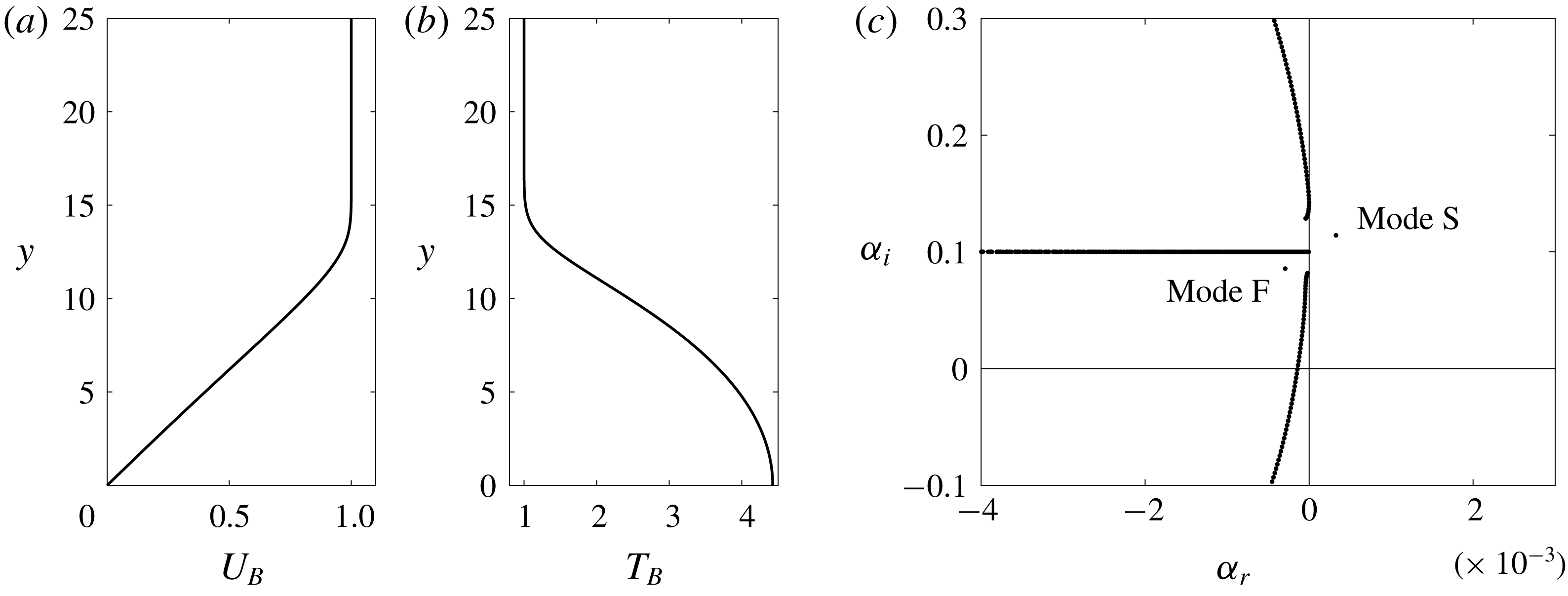
(a,b) Profiles of base velocity
 $U_{B}$
and temperature
 $T_{B}$
in the wall-normal direction
 $y$
for adiabatic high-speed boundary layer at
 $M_{0}=4.5$
. (c) Eigenvalue spectrum for
 $M_{0}=4.5$
,
 $Re_{0}=2000$
,
 $F=50$
and
 $b=0$
.

We first consider a steady laminar base state with streamwise velocity
 $U_{B}$
and temperature
 $T_{B}$
, which are obtained by solving the similarity equations (2.7)–(2.8) with an adiabatic boundary condition (
 $\unicode[STIX]{x2202}T_{B}/\unicode[STIX]{x2202}y=0$
at
 $y=0$
). Figure 1(a) shows
 $U_{B}(y)$
, with boundary-layer thickness
 $\unicode[STIX]{x1D6FF}_{99}=13.6$
and displacement thickness
 $\unicode[STIX]{x1D6FF}^{\ast }=10.5$
; figure 1(b) shows
 $T_{B}(y)$
, which has a thermal boundary-layer thickness
 $\unicode[STIX]{x1D703}_{99}=14.7$
and the wall temperature
 $T_{w}=4.43$
. Solution of the eigenvalue problem (2.15) at
 $Re_{0}=2000$
,
 $F=50$
and
 $b=0$
yields the eigenvalue spectrum in figure 1(c). Typical characteristics of the spectrum are observed: discrete modes denoted F and S, continuous branches of acoustic modes and overlapped continuous branches of vorticity and entropy modes which are aligned horizontally near
 $\unicode[STIX]{x1D6FC}_{i}=\unicode[STIX]{x1D714}=Re_{0}F/10^{6}=0.1$
(Balakumar & Malik Reference Balakumar and Malik1992; Joo & Durbin Reference Joo and Durbin2012). Mode S has a complex wavenumber
 $\unicode[STIX]{x1D6FC}=3.277\times 10^{-4}+0.1142\text{i}$
, and its phase speed
 $c=\unicode[STIX]{x1D714}/\unicode[STIX]{x1D6FC}_{i}=0.8756$
is slower than the free-stream velocity; Mode F has
 $\unicode[STIX]{x1D6FC}=-2.911\times 10^{-4}+0.0856\text{i}$
and its phase speed
 $c=1.1674$
is faster than the free stream.
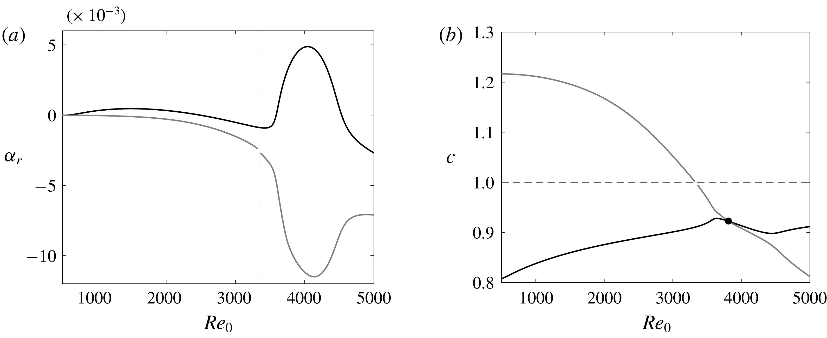
(a) Growth rate
 $\unicode[STIX]{x1D6FC}_{r}$
and (b) phase speed
 $c$
as a function of the Reynolds number
 $Re_{0}$
for the mode S (black) and the mode F (grey) for
 $M_{0}=4.5$
,
 $F=50$
and
 $b=0$
. Dashed lines indicate where the phase speed of the mode F becomes unity, and black dot in (b) indicates the synchronization point where the phase speeds of the modes S and F are equal.

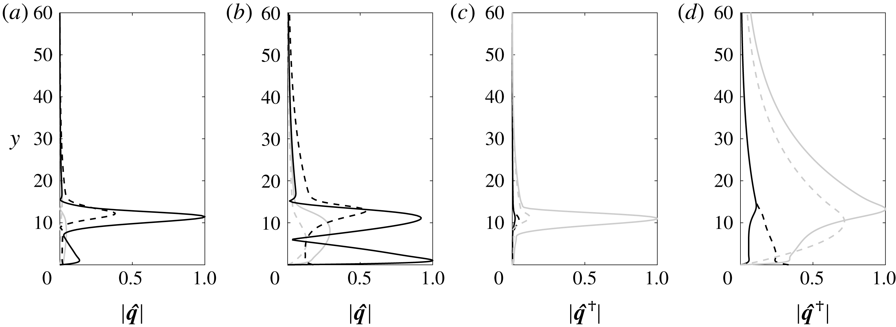
(a,b) Eigenfunctions
 $|\hat{\boldsymbol{q}}|$
with components
 $|\hat{T}|$
(black solid),
 $|\hat{\unicode[STIX]{x1D70C}}|$
(black dashed),
 $|\hat{u} |$
(grey solid),
 $|\hat{v}|$
(grey dashed) and (c,d) adjoint eigenfunctions
 $|\hat{\boldsymbol{q}}^{\dagger }|$
with components
 $|\hat{T}^{\dagger }|$
(black solid),
 $|\hat{\unicode[STIX]{x1D70C}}^{\dagger }|$
(black dashed),
 $|\hat{u} ^{\dagger }|$
(grey solid),
 $|\hat{v}^{\dagger }|$
(grey dashed) for the mode S (a,c) and the mode F (b,d) in figure 2(a) at
 $Re_{0}=2000$
. The eigenfunctions are normalized by the maximum of
 $|\hat{T}|$
while the adjoint eigenfunctions are normalized by the maximum of
 $|\hat{u} ^{\dagger }|$
.

The spatial growth rates
 $\unicode[STIX]{x1D6FC}_{r}$
and phase speeds
 $c$
of modes F and S are plotted as a function of Reynolds number
 $Re_{0}$
in figure 2. Mode S has the first unstable region in the range
 $590\lesssim Re_{0}\lesssim 2480$
and the second unstable region in the range
 $3590\lesssim Re_{0}\lesssim 4540$
, while mode F is always stable over this range of
 $Re_{0}$
. It is well established that mode S appears at low Reynolds number near the slow acoustic mode with a phase speed
 $c=1-1/M_{0}$
, while the mode F appears near the fast acoustic mode with phase speed
 $c=1+1/M_{0}$
(Fedorov & Khokhlov Reference Fedorov and Khokhlov2001; Fedorov Reference Fedorov2011; Fedorov & Tumin Reference Fedorov and Tumin2011). The phase speed of the former increases with
 $Re_{0}$
while that of the latter decreases, and they become equal in the synchronization region around
 $Re_{0}\simeq 3820$
. Fedorov & Tumin (Reference Fedorov and Tumin2011) suggested a model that describes the instability around the synchronization point due to mode crossing captured in figure 2. Beyond
 $Re_{0}\simeq 3340$
, the phase speed of mode F becomes less than unity and a discontinuity in
 $\unicode[STIX]{x1D6FC}$
is observed due to a synchronization between mode F and the continuous branch of entropy and vorticity modes. This modal exchange can be important for transition triggered by mode F (Fedorov Reference Fedorov2011). The eigenfunctions associated with modes S and F are shown in figure 3(a,b), and the corresponding adjoint eigenfunctions are plotted in figure 3(c,d). The perturbation temperature
 $\hat{T}$
is the largest component for both modes while the largest component in the adjoint eigenfunction is
 $\hat{u} ^{\dagger }$
. These forward and adjoint eigenfunctions,
 $\hat{\boldsymbol{q}}$
and
 $\hat{\boldsymbol{q}}^{\dagger }$
, will be used to evaluate the sensitivity profiles,
 $\unicode[STIX]{x1D735}_{\boldsymbol{Q}}\unicode[STIX]{x1D6FC}$
.
3.1 Sensitivity profiles
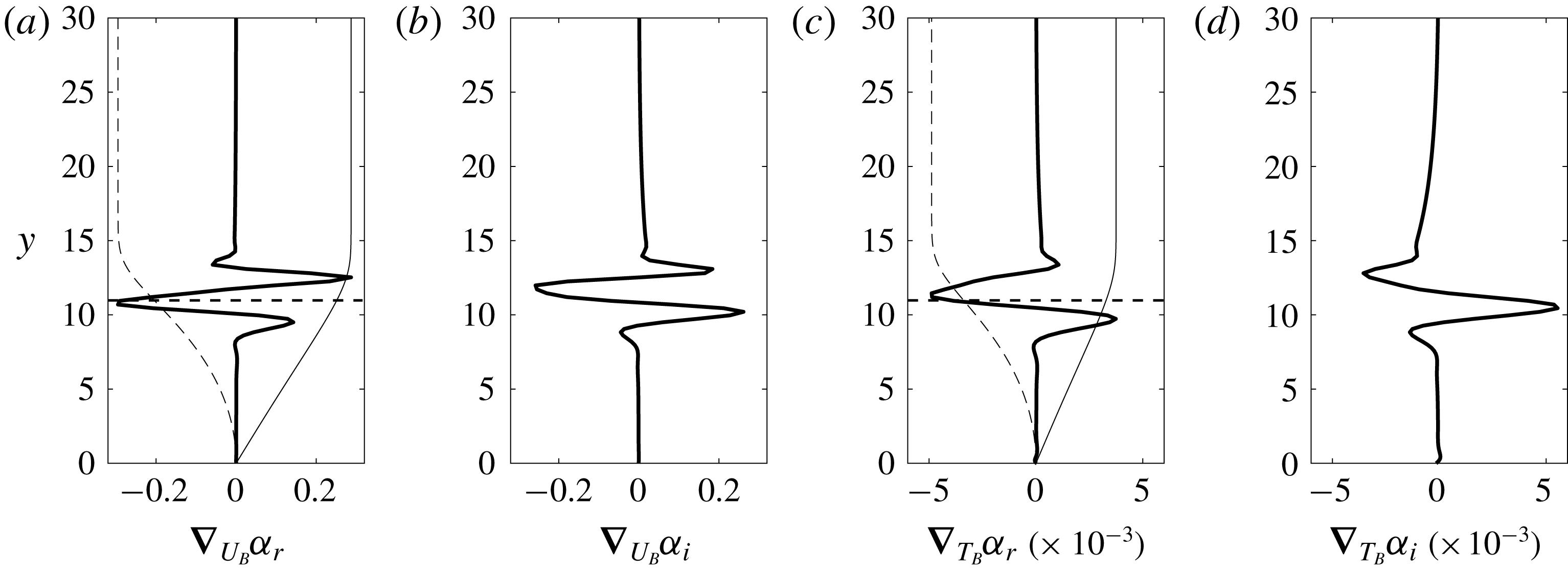
The sensitivity profiles of mode S are evaluated using equation (2.23) and are plotted in figure 4. They are decomposed into real and imaginary parts:
 $\unicode[STIX]{x1D735}_{U_{B}}\unicode[STIX]{x1D6FC}=\unicode[STIX]{x1D735}_{U_{B}}\unicode[STIX]{x1D6FC}_{r}+\text{i}\unicode[STIX]{x1D735}_{U_{B}}\unicode[STIX]{x1D6FC}_{i}$
and
 $\unicode[STIX]{x1D735}_{T_{B}}\unicode[STIX]{x1D6FC}=\unicode[STIX]{x1D735}_{T_{B}}\unicode[STIX]{x1D6FC}_{r}+\text{i}\unicode[STIX]{x1D735}_{T_{B}}\unicode[STIX]{x1D6FC}_{i}$
, where the real part is the sensitivity of the growth rate and the imaginary part is the sensitivity of streamwise wavenumber. In (a,c), we also display rescaled profiles of
 $U_{B}$
and
 $T_{B}$
to indicate where the sensitive region lies relative to the boundary-layer thicknesses. The profiles all oscillate in the wall-normal coordinate, and the sensitivity is small near the wall
 $y=0$
and in the free stream
 $y\rightarrow \infty$
; it is large immediately below the boundary-layer thickness
 $y_{99}$
. Specifically, the sensitivities
 $\unicode[STIX]{x1D735}_{U_{B}}\unicode[STIX]{x1D6FC}_{r}$
and
 $\unicode[STIX]{x1D735}_{T_{B}}\unicode[STIX]{x1D6FC}_{r}$
are large and negative near the critical layer
 $y_{c}$
, where the phase speed of mode S equals the base-flow velocity (i.e.
 $U_{B}(y_{c})=c$
). For
 $\unicode[STIX]{x1D735}_{U_{B}}\unicode[STIX]{x1D6FC}_{r}$
, there are two heights with positive sensitivity, one near
 $\unicode[STIX]{x1D6FF}_{99}$
and the other just below
 $y=10$
. Also
 $\unicode[STIX]{x1D735}_{T_{B}}\unicode[STIX]{x1D6FC}_{r}$
is positive just below
 $y=10$
and positive but small near
 $y=\unicode[STIX]{x1D6FF}_{99}$
. It is important to note that
 $\unicode[STIX]{x1D735}_{U_{B}}\unicode[STIX]{x1D6FC}$
is larger than
 $\unicode[STIX]{x1D735}_{T_{B}}\unicode[STIX]{x1D6FC}$
by orders of magnitude. Uncertainties in the base velocity are thus more influential with respect to stability, compared to uncertainties in the base temperature. The sensitivity profiles for three-dimensional instability waves (i.e.
 $\unicode[STIX]{x1D6FD}>0$
) are qualitatively similar to those in figure 4.
(a) Real and (b) imaginary parts of the sensitivity to base-velocity distortion
 $\unicode[STIX]{x1D735}_{U_{B}}\unicode[STIX]{x1D6FC}$
, and (c) real and (d) imaginary parts of the sensitivity to base-temperature distortion
 $\unicode[STIX]{x1D735}_{T_{B}}\unicode[STIX]{x1D6FC}$
for the mode S at
 $Re_{0}=2000$
. Thin solid and dashed linear lines represent properly scaled base velocity
 $U_{B}$
and temperature
 $T_{B}$
, and horizontal dashed lines represent the critical layer
 $y_{c}$
, respectively.

(a) The growth-rate sensitivity to base-velocity distortion
 $\unicode[STIX]{x1D735}_{U_{B}}\unicode[STIX]{x1D6FC}_{r}$
(grey lines), and (b–d) the real part of components
 $\hat{\boldsymbol{S}}_{U_{B}}^{1-3}$
(black lines) for the mode S at
 $Re_{0}=2000$
. Dotted, solid, dashed and dash-dot lines in (a) represent thermal boundary-layer thickness
 $\unicode[STIX]{x1D703}_{99}$
, boundary-layer thickness
 $\unicode[STIX]{x1D6FF}_{99}$
, critical layer
 $y_{c}$
and displacement thickness
 $\unicode[STIX]{x1D6FF}^{\ast }$
, respectively.

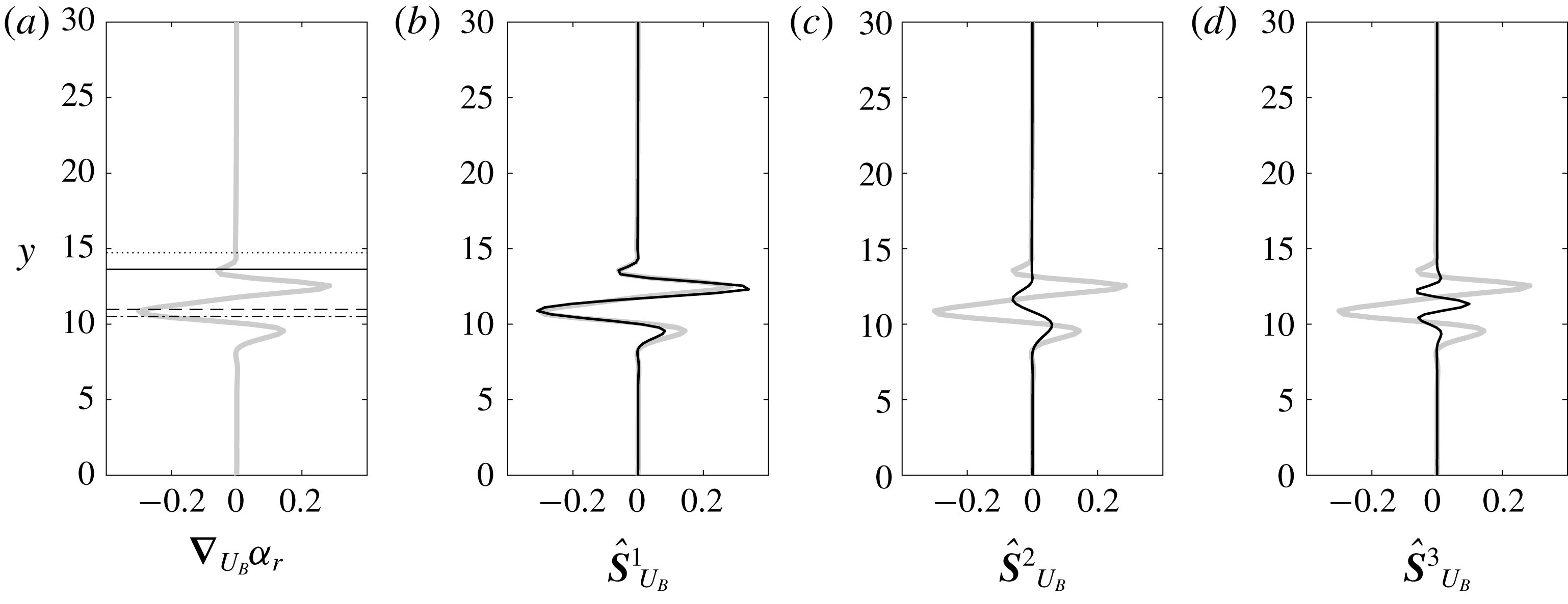
In figure 5, we decompose
 $\unicode[STIX]{x1D735}_{U_{B}}\unicode[STIX]{x1D6FC}_{r}$
into its constituents
 $\hat{\boldsymbol{S}}_{U_{B}}^{1-3}$
to assess the importance of each contribution. Note that the term
 $\hat{\boldsymbol{S}}_{U_{B}}^{4}$
is zero since it is due to streamwise variation of
 $U_{B}$
in the pressure dilation in the energy equation, and hence is not plotted. The real part of
 $\hat{\boldsymbol{S}}_{U_{B}}^{1}=\unicode[STIX]{x2202}/\unicode[STIX]{x2202}y(\unicode[STIX]{x1D70C}_{B}\hat{v}^{\ast }\hat{u} ^{\dagger })$
, which arises from the variation in
 $U_{B}$
altering the mean shear
 $\unicode[STIX]{x1D70C}_{B}(\unicode[STIX]{x2202}U_{B}/\unicode[STIX]{x2202}y)$
in the streamwise momentum equation, has a very similar profile to
 $\unicode[STIX]{x1D735}_{U_{B}}\unicode[STIX]{x1D6FC}_{r}$
; the other terms,
 $\hat{\boldsymbol{S}}_{U_{B}}^{2}$
and
 $\hat{\boldsymbol{S}}_{U_{B}}^{3}$
, have a relatively small amplitude. The results demonstrate that
 $\hat{\boldsymbol{S}}_{U_{B}}^{1}$
is the dominant term. Moreover,
 $\unicode[STIX]{x1D735}_{U_{B}}\unicode[STIX]{x1D6FC}_{r}$
and the real part of
 $\hat{\boldsymbol{S}}_{U_{B}}^{1}$
are largely negative near the critical layer
 $y_{c}$
where the change in vorticity gradient
 $\unicode[STIX]{x2202}^{2}U_{B}/\unicode[STIX]{x2202}y^{2}$
can significantly affect stability, due to the singular term in the inviscid limit. For instance, if we allow a positive distortion
 $\unicode[STIX]{x1D6FF}U_{B}>0$
narrowly around
 $y_{c}$
, the vorticity gradient around
 $y_{c}$
is negative (i.e.
 $\unicode[STIX]{x2202}^{2}(\unicode[STIX]{x1D6FF}U_{B})/\unicode[STIX]{x2202}y^{2}<0$
) and stabilizes the mode.
(a) The growth-rate sensitivity to base-temperature distortion
 $\unicode[STIX]{x1D735}_{T_{B}}\unicode[STIX]{x1D6FC}_{r}$
(grey lines), and (b–h) the real part of components
 $\hat{\boldsymbol{S}}_{T_{B}}^{1-7}$
(black lines) for the mode S at
 $Re_{0}=2000$
.

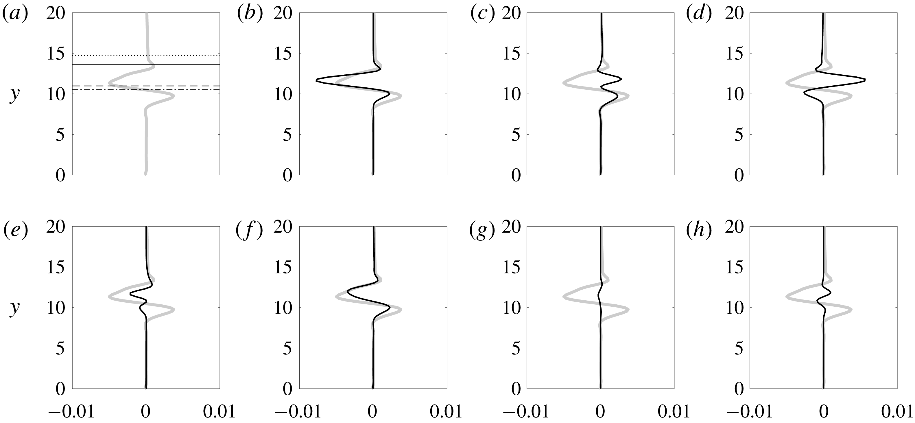
Figure 6 displays the total growth-rate sensitivity to base-temperature distortion
 $\unicode[STIX]{x1D735}_{T_{B}}\unicode[STIX]{x1D6FC}_{r}$
and the real part of the sensitivity components
 $\hat{\boldsymbol{S}}_{T_{B}}^{1-7}$
. In this case,
 $\hat{\boldsymbol{S}}_{T_{B}}^{8}$
is zero because it is associated with the variation of the base state in the streamwise direction. The real part
 $\hat{\boldsymbol{S}}_{T_{B}}^{1}=(\unicode[STIX]{x2202}U_{B}/\unicode[STIX]{x2202}y)(\hat{v}^{\ast }\hat{u} ^{\dagger }/T_{B}^{2})$
, which arises due to the modification of the mean shear in the
 $u$
-momentum equation by
 $\unicode[STIX]{x1D6FF}T_{B}$
, is similar to the total profile
 $\unicode[STIX]{x1D735}_{T_{B}}\unicode[STIX]{x1D6FC}_{r}$
. But we see that other components also have an appreciable amplitude, for example
 $\hat{\boldsymbol{S}}_{T_{B}}^{3}=[\unicode[STIX]{x1D6FC}^{\ast }\hat{u} ^{\ast }\hat{\unicode[STIX]{x1D70C}}^{\dagger }-\hat{v}^{\ast }(\unicode[STIX]{x2202}\hat{\unicode[STIX]{x1D70C}}^{\dagger }/\unicode[STIX]{x2202}y)-\text{i}\unicode[STIX]{x1D6FD}{\hat{w}}^{\ast }\hat{\unicode[STIX]{x1D70C}}^{\dagger }]/T_{B}^{2}$
which is the sensitivity due to base-density variation in the continuity equation, and
 $\hat{\boldsymbol{S}}_{T_{B}}^{5}=\unicode[STIX]{x1D70C}_{B}(\unicode[STIX]{x2202}/\unicode[STIX]{x2202}y)(\hat{v}^{\ast }\hat{T}^{\dagger })$
which is the sensitivity due to mean temperature-gradient terms in the energy equation. As the result, the growth-rate sensitivity
 $\unicode[STIX]{x1D735}_{T_{B}}\unicode[STIX]{x1D6FC}_{r}$
is due to combined influence of these multiple contributions from the continuity, momentum and energy equations; it is not dominated by any particular effect.
(a) Real and (b) imaginary parts of the sensitivity to base-velocity distortion
 $\unicode[STIX]{x1D735}_{U_{B}}\unicode[STIX]{x1D6FC}$
, and (c) real and (d) imaginary parts of the sensitivity to base-temperature distortion
 $\unicode[STIX]{x1D735}_{T_{B}}\unicode[STIX]{x1D6FC}$
for the mode F at
 $Re_{0}=2000$
.

Sensitivity profiles of the mode F at
 $Re_{0}=4000$
. Dashed lines denote the critical layer
 $y_{c}$
of the mode F.

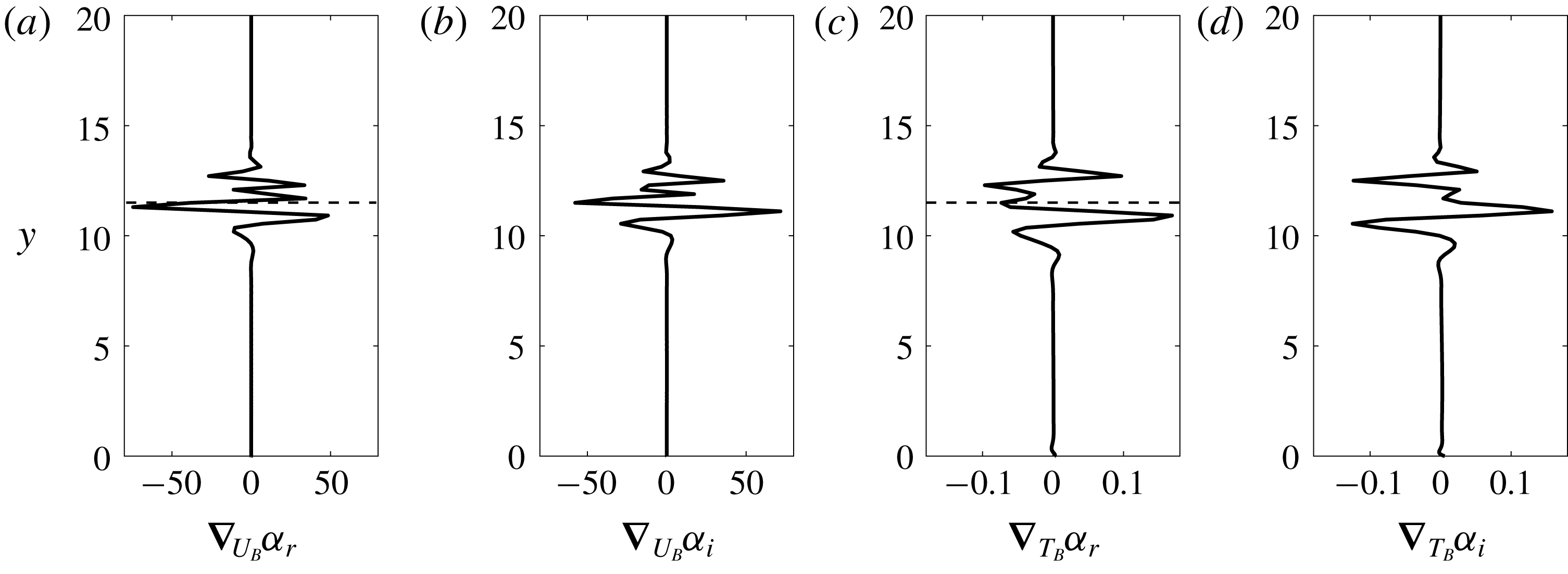
Now we turn our attention to the sensitivity of the fast mode F, which is plotted in figure 7 at low Reynolds number
 $Re_{0}=2000$
. Compared to mode S, very small sensitivity to
 $\unicode[STIX]{x1D6FF}U_{B}$
and
 $\unicode[STIX]{x1D6FF}T_{B}$
is observed above the boundary-layer thickness, and the profile is less oscillatory. The weak sensitivity can be ascribed to mode F not having a critical layer at
 $Re_{0}=2000$
since its phase speed
 $c$
is larger than unity. As a result, at
 $Re_{0}=4000$
when mode F has a critical layer at
 $y_{c}=11.5$
, its sensitivity profiles are very different (see figure 8): they become oscillatory and are appreciably larger in amplitude. The value of
 $\unicode[STIX]{x1D735}_{U_{B}}\unicode[STIX]{x1D6FC}_{r}$
is negative at the critical layer, and
 $\unicode[STIX]{x1D735}_{U_{B}}\unicode[STIX]{x1D6FC}$
is orders of magnitude larger than
 $\unicode[STIX]{x1D735}_{T_{B}}\unicode[STIX]{x1D6FC}$
– both observations similar to mode S.
3.2 Parametric study
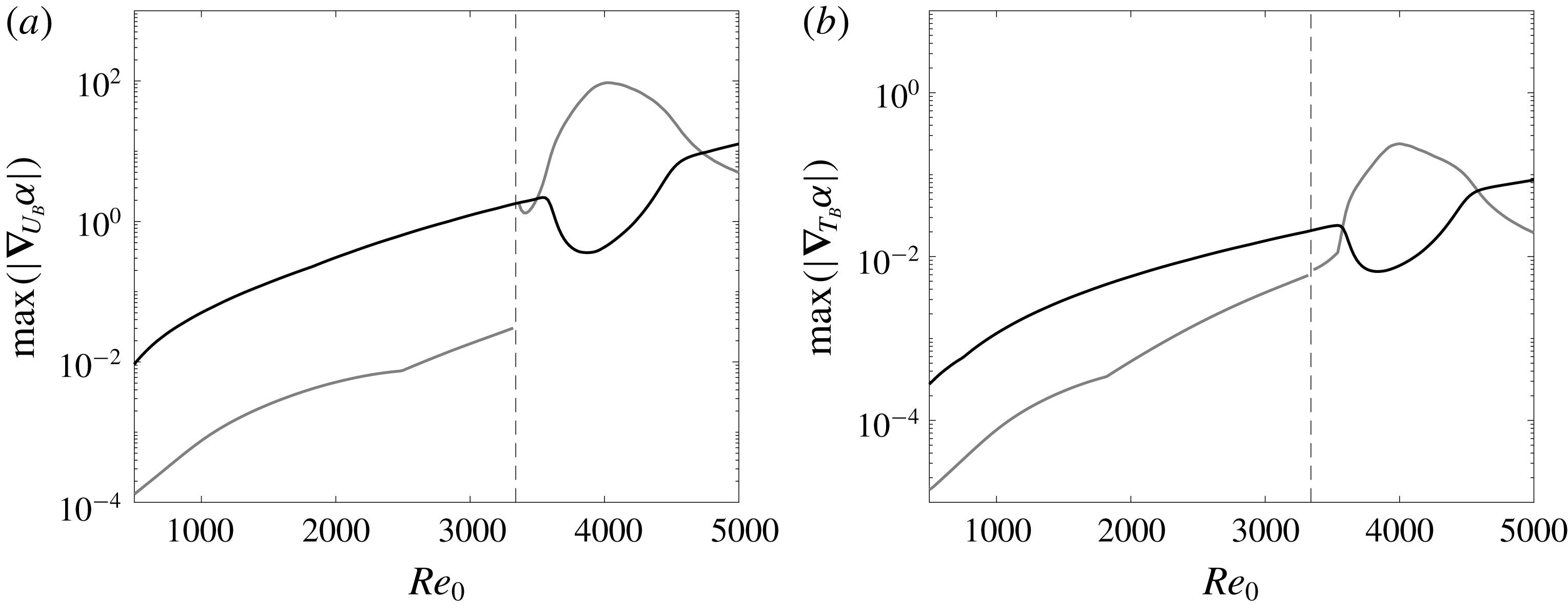
The sensitivities of modes S and F vary with the parameters of the flow and the instability wave, for example the Reynolds number and the wavenumber of the modes. Figure 9 focuses on the effect of the Reynolds number. The wall-normal maxima in the sensitivity profiles,
 $|\unicode[STIX]{x1D735}_{U_{B}}\unicode[STIX]{x1D6FC}|$
and
 $|\unicode[STIX]{x1D735}_{T_{B}}\unicode[STIX]{x1D6FC}|$
, are plotted versus
 $Re_{0}$
. In general, the sensitivities increase with Reynolds number and
 $\unicode[STIX]{x1D735}_{U_{B}}\unicode[STIX]{x1D6FC}$
is always substantially larger than
 $\unicode[STIX]{x1D735}_{T_{B}}\unicode[STIX]{x1D6FC}$
. At low
 $Re_{0}$
, mode S has a much larger sensitivity than mode F.
Maximum in
 $y$
-direction of the sensitivity (a)
 $|\unicode[STIX]{x1D735}_{U_{B}}\unicode[STIX]{x1D6FC}|$
and (b)
 $|\unicode[STIX]{x1D735}_{T_{B}}\unicode[STIX]{x1D6FC}|$
as a function of the Reynolds number for the modes S (black) and F (grey). Dashed lines denote the Reynolds number where the phase speed of the mode F becomes unity.

Around
 $Re_{0}=3340$
, mode F coalesces with the continuous vorticity/entropy branches (Fedorov & Khokhlov Reference Fedorov and Khokhlov2001), and the LST solution at this point is not achievable and hence neither is its sensitivity. Away from this point, however, LST analysis of mode F is valid and the sensitivity formulation is therefore applicable. The discontinuous jump in the sensitivity of that mode takes place when its phase speed becomes less than unity and its critical layer is established. The two modes F and S become synchronous at
 $Re_{0}\simeq 3820$
; while the stability operator can be expanded differently in the vicinity of this point (Fedorov & Khokhlov Reference Fedorov and Khokhlov2001), such expansion is applicable for locally varying solutions. Therefore, the LST and sensitivity results presented herein are not affected. Over the range
 $3600\leqslant Re_{0}\leqslant 4600$
, the sensitivity of mode F increases rapidly, and surpasses the sensitivity of mode S which is reduced. In this regime, the temperature eigenfunction
 $\hat{T}(y)$
of the latter mode changes appreciably, but its impact on sensitivity was not possible to isolate because
 $(\hat{\unicode[STIX]{x1D70C}},\hat{u} ,\hat{v})$
also change.
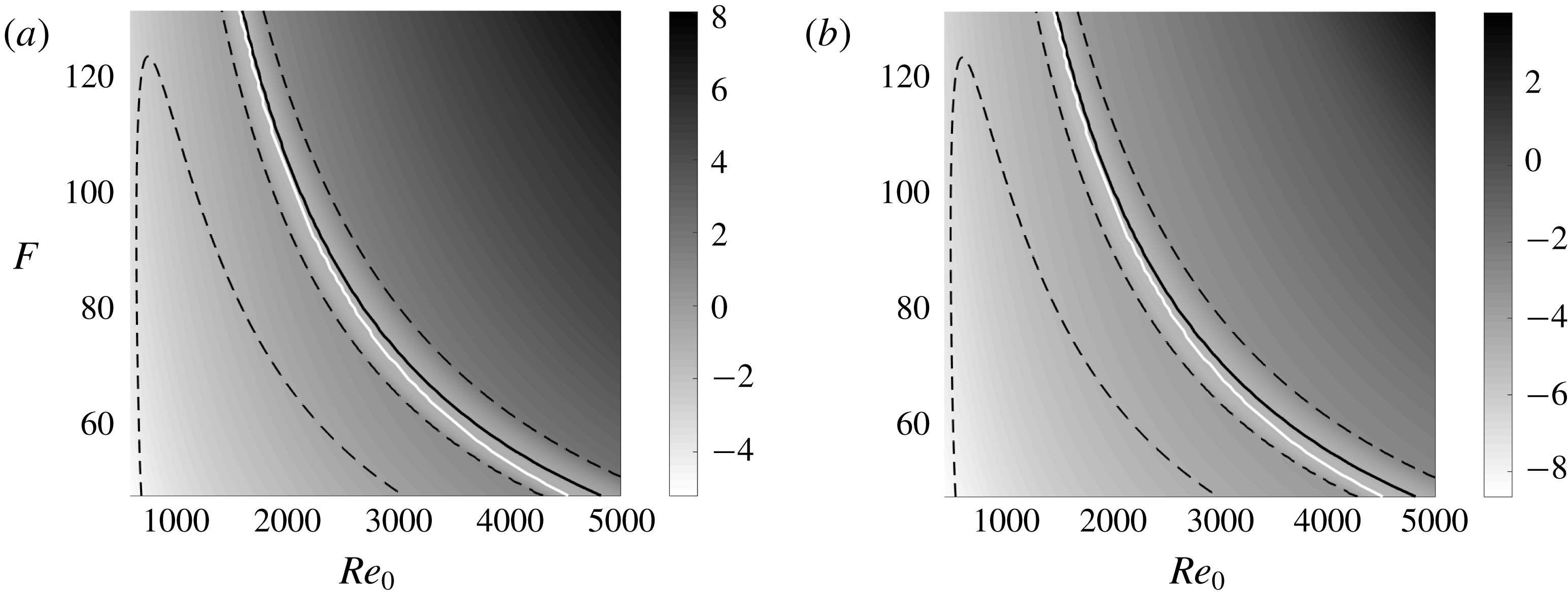
Contours of the maximum of sensitivity functions (a)
 $\log (\max |\unicode[STIX]{x1D735}_{U_{B}}\unicode[STIX]{x1D6FC}|)$
and (b)
 $\log (\max |\unicode[STIX]{x1D735}_{T_{B}}\unicode[STIX]{x1D6FC}|)$
for the mode S in the parameter space
 $(Re_{0},F)$
. Dashed lines represent the neutral stability curve where
 $\unicode[STIX]{x1D6FC}_{r}=0$
; black solid lines represent the location where the growth rate
 $\unicode[STIX]{x1D6FC}_{r}$
is maximum; white solid lines represent the synchronization condition where the phase speeds of modes F and S are equal.

Figure 10 shows contours of the maximum sensitivity of the two-dimensional mode S to
 $\unicode[STIX]{x1D6FF}U_{B}$
and
 $\unicode[STIX]{x1D6FF}T_{B}$
, as a function of the Reynolds number
 $Re_{0}$
and the non-dimensional frequency
 $F$
. The earlier trend shown in figure 9 for
 $F=50$
is observed at other frequencies: both
 $\unicode[STIX]{x1D735}_{U_{B}}\unicode[STIX]{x1D6FC}$
and
 $\unicode[STIX]{x1D735}_{T_{B}}\unicode[STIX]{x1D6FC}$
increase with
 $Re_{0}$
and drop transiently near the synchronization point. Dashed lines indicate neutral stability for mode S, and the solid line marks where the two-dimensional mode S is most unstable. The maximum growth rate coincides with the local minimum sensitivity. We also see that
 $\unicode[STIX]{x1D735}_{U_{B}}\unicode[STIX]{x1D6FC}$
is larger than
 $\unicode[STIX]{x1D735}_{T_{B}}\unicode[STIX]{x1D6FC}$
in orders of magnitude in all of the parameter space of
 $Re_{0}$
and
 $F$
.
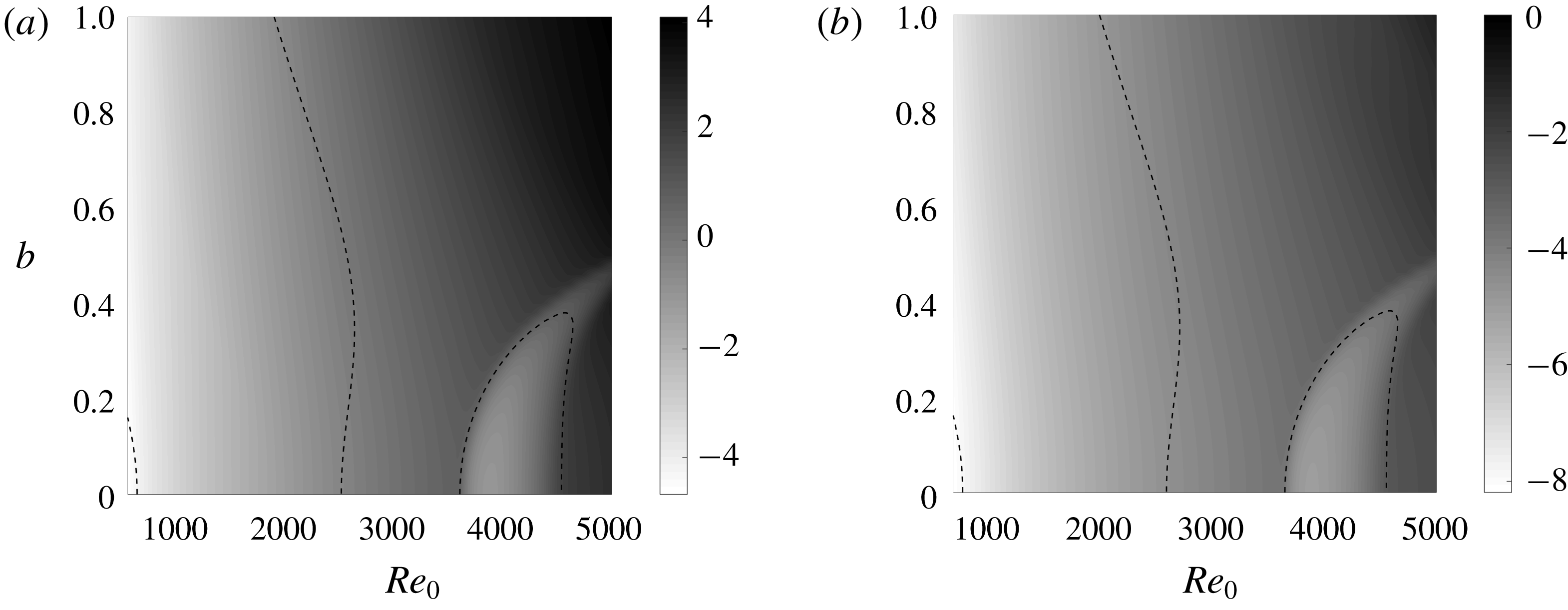
Contours of the maximum of sensitivity functions (a)
 $\log (\max |\unicode[STIX]{x1D735}_{U_{B}}\unicode[STIX]{x1D6FC}|)$
and (b)
 $\log (\max |\unicode[STIX]{x1D735}_{T_{B}}\unicode[STIX]{x1D6FC}|)$
of the mode S in the parameter space
 $(Re_{0},b)$
. Dashed lines represent the neutral stability curve where
 $\unicode[STIX]{x1D6FC}_{r}=0$
.

The effect of three-dimensionality of mode S is examined in figure 11 where contours of the maximum sensitivities are plotted versus
 $Re_{0}$
and
 $b=\unicode[STIX]{x1D6FD}/Re_{0}\times 10^{4}$
, at
 $F=50$
. The growth rate of the mode reaches a maximum around
 $Re_{0}=4000$
when
 $b=0$
; for
 $b>0.4$
, the first unstable region moves upstream and the second unstable region disappears. At a fixed
 $b$
, the sensitivity increases with
 $Re_{0}$
, but drops suddenly in the second unstable region
 $b<0.4$
. At a fixed
 $Re_{0}$
, the sensitivity shows weak dependence on
 $b$
. Over the entire parameter space,
 $\unicode[STIX]{x1D735}_{U_{B}}\unicode[STIX]{x1D6FC}$
is larger than
 $\unicode[STIX]{x1D735}_{T_{B}}\unicode[STIX]{x1D6FC}$
by approximately four orders of magnitude.
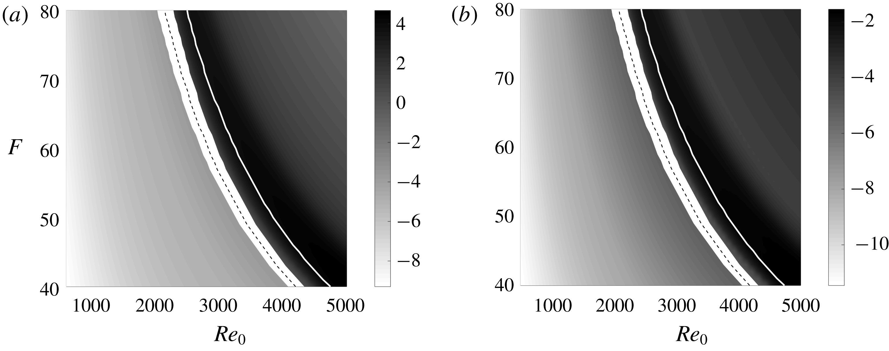
Contours of the maximum of sensitivity functions (a)
 $\log (\max |\unicode[STIX]{x1D735}_{U_{B}}\unicode[STIX]{x1D6FC}|)$
and (b)
 $\log (\max |\unicode[STIX]{x1D735}_{T_{B}}\unicode[STIX]{x1D6FC}|)$
of the mode F in the parameter space
 $(Re_{0},F)$
. Dashed lines in white area represent the location where the phase speed of the mode F becomes unity, and white solid lines represent the synchronization point where the phase speed of the mode F equals to that of the mode S.

The sensitivity of the mode F is also examined as a function of
 $(Re_{0},F)$
, and contours of the maximum values of
 $\unicode[STIX]{x1D735}_{U_{B}}\unicode[STIX]{x1D6FC}$
and
 $\unicode[STIX]{x1D735}_{T_{B}}\unicode[STIX]{x1D6FC}$
are plotted in figure 12. The sharp jump in the sensitivity around the Reynolds number where the phase speed becomes unity (dashed line) is observed over the full range of frequencies considered. The increase in sensitivity in the vicinity of the synchronization point (white solid line) also persists. Similar to mode S, the sensitivity increases with frequency
 $F$
at a fixed
 $Re_{0}$
, and
 $\unicode[STIX]{x1D735}_{U_{B}}\unicode[STIX]{x1D6FC}$
is orders of magnitude larger than
 $\unicode[STIX]{x1D735}_{T_{B}}\unicode[STIX]{x1D6FC}$
.
3.3 Optimal base state
The sensitivity profiles
 $\unicode[STIX]{x1D735}_{U_{B}}\unicode[STIX]{x1D6FC}$
and
 $\unicode[STIX]{x1D735}_{T_{B}}\unicode[STIX]{x1D6FC}$
identify wall-normal heights at which the boundary-layer stability is most responsive to base-state distortions. For instance, local acceleration of
 $\unicode[STIX]{x1D6FF}U_{B}$
near the critical layer can effectively stabilize modes S and F. The question naturally arises as to what is the optimal distortion to the base state, which causes the largest change in flow stability. In the limit of a small distortion in incompressible flow, Bottaro et al. (Reference Bottaro, Corbett and Luchini2003) solved the optimization problem and showed that
 $\unicode[STIX]{x1D735}_{U_{B}}\unicode[STIX]{x1D6FC}_{r}$
, with appropriate scaling, is in fact the optimal modification
 $\unicode[STIX]{x1D6FF}U_{B}$
. The optimization problem is herein examined for compressible flows in order to evaluate the optimal base velocity
 $\bar{U}$
and temperature
 $\bar{T}$
. A Lagrangian approach is adopted, and we restrict the optimal base state
 $\bar{U}$
and
 $\bar{T}$
to satisfy the following energy constraints,
 $$\begin{eqnarray}J_{U}=\int _{0}^{\infty }\unicode[STIX]{x1D70C}_{B}(\bar{U}-U_{B})^{2}\,\text{d}y-r_{U}^{2}=0,\quad J_{T}=\int _{0}^{\infty }\frac{\unicode[STIX]{x1D70C}_{B}^{2}}{\unicode[STIX]{x1D6FE}_{0}(\unicode[STIX]{x1D6FE}_{0}-1)M_{0}^{2}}(\bar{T}-T_{B})^{2}\,\text{d}y-r_{T}^{2}=0,\end{eqnarray}$$
where
 $r_{U}$
and
 $r_{T}$
are the prescribed kinetic and thermal energy distortions, scaled similarly to the definition of the energy norm by Hanifi et al. (Reference Hanifi, Schmid and Henningson1996). We define the Lagrangian,
 $$\begin{eqnarray}\mathscr{L}=\unicode[STIX]{x1D6FC}-(\hat{\boldsymbol{q}}^{\dagger },(\unicode[STIX]{x1D6FC}{\mathcal{A}}+{\mathcal{B}})\hat{\boldsymbol{q}})+\unicode[STIX]{x1D706}_{U}J_{U}+\unicode[STIX]{x1D706}_{T}J_{T},\end{eqnarray}$$
where
 $\unicode[STIX]{x1D706}_{U}$
,
 $\unicode[STIX]{x1D706}_{T}$
and the adjoint eigenmode
 $\hat{\boldsymbol{q}}^{\dagger }$
are all Lagrange multipliers. In order to maximize
 $\unicode[STIX]{x1D6FC}$
, we seek stationary points of
 $\mathscr{L}$
. Differentiation with respect to
 $\unicode[STIX]{x1D706}_{U}$
and
 $\unicode[STIX]{x1D706}_{T}$
yields the constraints (3.3); differentiation with respect to the adjoint
 $\hat{\boldsymbol{q}}^{\dagger }$
yields the eigenvalue problem (2.15), and with respect to
 $\hat{\boldsymbol{q}}$
yields the adjoint equations (2.22); the derivative with respect to
 $\unicode[STIX]{x1D6FC}$
gives,
 $$\begin{eqnarray}\frac{\unicode[STIX]{x2202}\mathscr{L}}{\unicode[STIX]{x2202}\unicode[STIX]{x1D6FC}}=1-\left(\hat{\boldsymbol{q}}^{\dagger },\left({\mathcal{A}}+\unicode[STIX]{x1D6FC}\frac{\unicode[STIX]{x2202}{\mathcal{A}}}{\unicode[STIX]{x2202}\unicode[STIX]{x1D6FC}}\right)\hat{\boldsymbol{q}}\right)=0.\end{eqnarray}$$
Comparison of the above expression to (2.23) shows that the norm
 $\hat{R}$
is unity. In order to determine the optimal base state, we differentiate the Lagrangian
 $\mathscr{L}$
with respect to
 $\bar{U}$
and
 $\bar{T}$
,
 $$\begin{eqnarray}\displaystyle & \displaystyle \frac{\unicode[STIX]{x2202}\mathscr{L}}{\unicode[STIX]{x2202}\bar{U}}\unicode[STIX]{x1D6FF}U=-\!\underbrace{\left(\hat{\boldsymbol{q}}^{\dagger },\unicode[STIX]{x1D6FC}\frac{\unicode[STIX]{x2202}{\mathcal{A}}}{\unicode[STIX]{x2202}\bar{U}}\unicode[STIX]{x1D6FF}U\hat{\boldsymbol{q}}+\frac{\unicode[STIX]{x2202}{\mathcal{B}}}{\unicode[STIX]{x2202}\bar{U}}\unicode[STIX]{x1D6FF}U\hat{\boldsymbol{q}}\right)}_{=(\unicode[STIX]{x1D735}_{U_{B}}\unicode[STIX]{x1D6FC},\unicode[STIX]{x1D6FF}U)}+\,2\unicode[STIX]{x1D706}_{U}\int _{0}^{\infty }\unicode[STIX]{x1D70C}_{B}(\bar{U}-U_{B})\unicode[STIX]{x1D6FF}U\,\text{d}y=0, & \displaystyle\end{eqnarray}$$
 $$\begin{eqnarray}\displaystyle & \displaystyle \frac{\unicode[STIX]{x2202}\mathscr{L}}{\unicode[STIX]{x2202}\bar{T}}\unicode[STIX]{x1D6FF}T=-\!\underbrace{\left(\hat{\boldsymbol{q}}^{\dagger },\unicode[STIX]{x1D6FC}\frac{\unicode[STIX]{x2202}{\mathcal{A}}}{\unicode[STIX]{x2202}\bar{T}}\unicode[STIX]{x1D6FF}T\hat{\boldsymbol{q}}+\frac{\unicode[STIX]{x2202}{\mathcal{B}}}{\unicode[STIX]{x2202}\bar{T}}\unicode[STIX]{x1D6FF}T\hat{\boldsymbol{q}}\right)}_{=(\unicode[STIX]{x1D735}_{T_{B}}\unicode[STIX]{x1D6FC},\unicode[STIX]{x1D6FF}T)}+\,2\unicode[STIX]{x1D706}_{T}\int _{0}^{\infty }\frac{\unicode[STIX]{x1D70C}_{B}^{2}}{\unicode[STIX]{x1D6FE}_{0}(\unicode[STIX]{x1D6FE}_{0}-1)M_{0}^{2}}(\bar{T}-T_{B})\unicode[STIX]{x1D6FF}T\,\text{d}y=0. & \displaystyle \nonumber\\ \displaystyle & & \displaystyle\end{eqnarray}$$
Taking the real part of the sensitivities,
 $\unicode[STIX]{x1D735}_{U}\unicode[STIX]{x1D6FC}_{r}$
and
 $\unicode[STIX]{x1D735}_{T}\unicode[STIX]{x1D6FC}_{r}$
, leads to the optimal base state
 $$\begin{eqnarray}\bar{U}=U_{B}\pm \frac{T_{B}}{2\unicode[STIX]{x1D706}_{U}}\unicode[STIX]{x1D735}_{U_{B}}\unicode[STIX]{x1D6FC}_{r},\quad \bar{T}=T_{B}\pm \frac{\unicode[STIX]{x1D6FE}_{0}(\unicode[STIX]{x1D6FE}_{0}-1)M_{0}^{2}T_{B}^{2}}{2\unicode[STIX]{x1D706}_{T}}\unicode[STIX]{x1D735}_{T_{B}}\unicode[STIX]{x1D6FC}_{r},\end{eqnarray}$$
which maximizes the change in flow stability. The Lagrange multipliers
 $\unicode[STIX]{x1D706}_{U}$
and
 $\unicode[STIX]{x1D706}_{T}$
are determined from the constraints (3.3),
 $$\begin{eqnarray}\unicode[STIX]{x1D706}_{U}=\sqrt{\frac{1}{4r_{U}^{2}}\int _{0}^{\infty }T_{B}(\unicode[STIX]{x1D735}_{U}\unicode[STIX]{x1D6FC}_{r})^{2}\,\text{d}y},\quad \unicode[STIX]{x1D706}_{T}=\sqrt{\frac{\unicode[STIX]{x1D6FE}_{0}(\unicode[STIX]{x1D6FE}_{0}-1)M_{0}^{2}}{4r_{T}^{2}}\int _{0}^{\infty }T_{B}^{2}(\unicode[STIX]{x1D735}_{T_{B}}\unicode[STIX]{x1D6FC}_{r})^{2}\,\text{d}y}.\end{eqnarray}$$
The corresponding growth-rate distortion is then,
 $$\begin{eqnarray}\unicode[STIX]{x1D6FF}\unicode[STIX]{x1D6FC}_{r}|_{U}=\pm \sqrt{r_{U}^{2}\int _{0}^{\infty }T_{B}(\unicode[STIX]{x1D735}_{U_{B}}\unicode[STIX]{x1D6FC}_{r})^{2}\,\text{d}y},\quad \unicode[STIX]{x1D6FF}\unicode[STIX]{x1D6FC}_{r}|_{T}=\pm \sqrt{r_{T}^{2}\unicode[STIX]{x1D6FE}_{0}(\unicode[STIX]{x1D6FE}_{0}-1)M_{0}^{2}\int _{0}^{\infty }T_{B}^{2}(\unicode[STIX]{x1D735}_{T_{B}}\unicode[STIX]{x1D6FC}_{r})^{2}\,\text{d}y}.\end{eqnarray}$$
The sensitivity profiles
 $\unicode[STIX]{x1D735}_{U_{B}}\unicode[STIX]{x1D6FC}_{r}$
and
 $\unicode[STIX]{x1D735}_{T_{B}}\unicode[STIX]{x1D6FC}_{r}$
are thus, with appropriate scaling, the most destabilizing or stabilizing distortions
 $\unicode[STIX]{x1D6FF}U_{B}$
and
 $\unicode[STIX]{x1D6FF}T_{B}$
, respectively.
Similarly, taking the imaginary part of (3.6)–(3.7) gives the optimal base state
 $$\begin{eqnarray}\bar{U}=U_{B}\pm \frac{T_{B}}{2\unicode[STIX]{x1D706}_{U}}\unicode[STIX]{x1D735}_{U_{B}}\unicode[STIX]{x1D6FC}_{i},\quad \bar{T}=T_{B}\pm \frac{\unicode[STIX]{x1D6FE}_{0}(\unicode[STIX]{x1D6FE}_{0}-1)M_{0}^{2}T_{B}^{2}}{2\unicode[STIX]{x1D706}_{T}}\unicode[STIX]{x1D735}_{T_{B}}\unicode[STIX]{x1D6FC}_{i},\end{eqnarray}$$
which maximally distorts the streamwise wavenumber. The resulting changes in
 $\unicode[STIX]{x1D6FC}_{i}$
are,
 $$\begin{eqnarray}\unicode[STIX]{x1D6FF}\unicode[STIX]{x1D6FC}_{i}|_{U}=\pm \sqrt{r_{U}^{2}\int _{0}^{\infty }T_{B}(\unicode[STIX]{x1D735}_{U_{B}}\unicode[STIX]{x1D6FC}_{i})^{2}\,\text{d}y},\quad \unicode[STIX]{x1D6FF}\unicode[STIX]{x1D6FC}_{i}|_{T}=\pm \sqrt{r_{T}^{2}\unicode[STIX]{x1D6FE}_{0}(\unicode[STIX]{x1D6FE}_{0}-1)M_{0}^{2}\int _{0}^{\infty }T_{B}^{2}(\unicode[STIX]{x1D735}_{T_{B}}\unicode[STIX]{x1D6FC}_{i})^{2}\,\text{d}y}.\end{eqnarray}$$
The optimal base state (3.8) is valid when
 $r_{U}$
and
 $r_{T}$
are infinitesimal, and hence the distortions are small – a condition that is satisfied in the present work. Similar to Bottaro et al. (Reference Bottaro, Corbett and Luchini2003), while the reference state
 $(U_{B},T_{B})$
satisfies the boundary-layer similarity equations, we did not apply the same constraint to the distorted base state. This choice enabled the derivation of analytical expressions for the optimal base state, and the establishing of its relation to the sensitivity profile. For finite-amplitude distortions, and to constraint the optimal base state to satisfy the boundary-layer equations, the optimization problem must be solved numerically and iteratively.
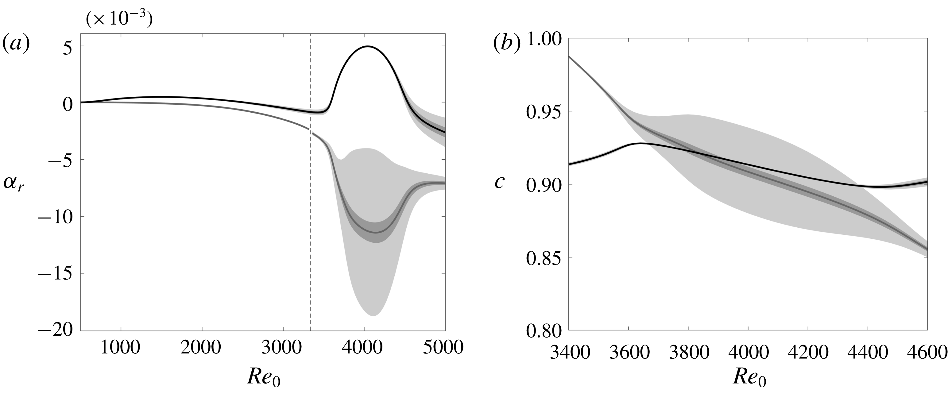
(a) Growth rate and (b) phase speed of the mode S (black solid lines) and the mode F (grey solid lines), and uncertainty bounds with
 $|r_{U}|\leqslant 10^{-4}$
,
 $r_{T}=0$
(light grey area), and
 $|r_{T}|\leqslant 10^{-3}$
,
 $r_{U}=0$
(dark grey area).

Figure 13 shows the growth rate
 $\unicode[STIX]{x1D6FC}_{r}$
and the phase speed
 $c$
of modes S and F, and the corresponding uncertainty bounds with
 $\unicode[STIX]{x1D6FC}_{r}\pm \unicode[STIX]{x1D6FF}\unicode[STIX]{x1D6FC}_{r}$
and
 $c\pm \unicode[STIX]{x1D6FF}c=\unicode[STIX]{x1D714}/(\unicode[STIX]{x1D6FC}_{i}\pm \unicode[STIX]{x1D6FF}\unicode[STIX]{x1D6FC}_{i})$
. The deviations
 $\unicode[STIX]{x1D6FF}\unicode[STIX]{x1D6FC}_{r}$
and
 $\unicode[STIX]{x1D6FF}\unicode[STIX]{x1D6FC}_{i}$
are evaluated from (3.10) and (3.12). The light grey bands represent the uncertainty bounds when
 $|r_{U}|\leqslant 10^{-4}$
and
 $r_{T}=0$
, while the dark grey are the uncertainty bounds when
 $r_{U}=0$
and
 $|r_{T}|\leqslant 10^{-3}$
. It is remarkable that such a small energy of the base state modification, of the order of
 $O(10^{-6}{-}10^{-8})$
, yields significant changes in the growth rates and phase speeds. In particular, mode F has very large uncertainty bounds after its phase speed becomes less than unity. Not only does its growth rate change substantially, but also the synchronization Reynolds number becomes uncertain (
 $3670\lesssim Re_{0}\lesssim 4380$
). Since the sensitivity
 $\unicode[STIX]{x1D735}_{T_{B}}\unicode[STIX]{x1D6FC}$
is orders of magnitude smaller than
 $\unicode[STIX]{x1D735}_{U_{B}}\unicode[STIX]{x1D6FC}$
, a larger value of
 $r_{T}$
remains relatively benign in terms of its impact on the growth rate and phase speed.
Perturbations of (a) velocity
 $u$
and (c) temperature
 $T$
, and mode shapes (b)
 $|{\check{u}}|$
and (d)
 $|{\check{T}}|$
from the PSE computation of the mode S for
 $M_{0}=4.5$
and
 $F=50$
. Solid, dashed and dash-dot lines denote the boundary-layer thickness
 $\unicode[STIX]{x1D6FF}_{99}$
, the critical layer
 $y_{c}$
and the displacement thickness
 $\unicode[STIX]{x1D6FF}^{\ast }$
, respectively. For clarity, the perturbations in (a,c) are plotted in a small portion of the domain, which is identified by the grey rectangles in (b,d).

4 Sensitivity in spatially developing boundary layers
4.1 PSE solution and its sensitivity
In this section, we investigate the sensitivity of spatially developing boundary layers to base-state distortion using the PSE. We focus on the sensitivity of the mode S, both in terms of its growth rate and the
 $N$
-factor. Figure 14 shows perturbations
 $u$
and
 $T$
and the corresponding mode shapes
 ${\check{u}}$
and
 ${\check{T}}$
of mode S at
 $F=50$
. The inflow condition for the PSE is obtained from the LST results at
 $Re_{0}=750$
. We only display the perturbation in the downstream portion of the domain in order to highlight the development of the instability wave. The most energetic component is the perturbation temperature
 $T$
which is mostly localized near the critical layer
 $y_{c}$
. The perturbation
 $u$
, on the other hand, is localized below
 $y_{c}$
. Figure 14(b,d) shows the corresponding mode shapes
 ${\check{u}}$
and
 ${\check{T}}$
. Overall, they shift upward and their amplitudes decrease as the boundary layer develops downstream. The adjoint perturbations
 $u^{\dagger }$
and
 $T^{\dagger }$
are displayed in figure 15(a,c). Since the unstable mode S grows downstream, the adjoint mode grows upstream, and therefore only the region near the inflow is displayed in the figure for clarity. Among the adjoint perturbation components,
 $u^{\dagger }$
is most energetic. The adjoint mode shapes
 ${\check{u}}^{\dagger }$
and
 ${\check{T}}^{\dagger }$
are also displayed in figure 15(b,d). Their amplitude grows along the boundary-layer thickness, similar to
 ${\check{T}}$
.
Adjoint perturbations (a)
 $u^{\dagger }$
and (c)
 $T^{\dagger }$
, and adjoint mode shapes (b)
 $|{\check{u}}^{\dagger }|$
and (d)
 $|{\check{T}}^{\dagger }|$
from the adjoint PSE. For clarity, the adjoint perturbations in (a,c) are plotted in a short portion of the domain, which is identified by the grey rectangles in (b,d).

(a–c) Two-dimensional profiles of the growth rate sensitivity for the mode S: (a)
 $\unicode[STIX]{x1D735}_{U_{B}}\unicode[STIX]{x1D6FE}_{r}$
, (b)
 $\unicode[STIX]{x1D735}_{V_{B}}\unicode[STIX]{x1D6FE}_{r}$
and (c)
 $\unicode[STIX]{x1D735}_{T_{B}}\unicode[STIX]{x1D6FE}_{r}$
. Solid, dashed and dash-dot lines denote the boundary-layer thickness
 $\unicode[STIX]{x1D6FF}_{99}$
, the critical layer
 $y_{c}$
and the displacement thickness
 $\unicode[STIX]{x1D6FF}^{\ast }$
, respectively. (d) Maximum sensitivity in
 $y$
-direction versus
 $x$
for
 $\max (|\unicode[STIX]{x1D735}_{U_{B}}\unicode[STIX]{x1D6FE}|)$
(black solid),
 $\max (|\unicode[STIX]{x1D735}_{V_{B}}\unicode[STIX]{x1D6FE}|)$
(grey solid) and
 $\max (|\unicode[STIX]{x1D735}_{T_{B}}\unicode[STIX]{x1D6FE}|)$
(light grey solid). Dashed lines are the rescaled maximum sensitivity functions
 $|\unicode[STIX]{x1D735}_{U_{B}}\unicode[STIX]{x1D6FC}|$
and
 $|\unicode[STIX]{x1D735}_{T_{B}}\unicode[STIX]{x1D6FC}|$
from the LST in figure 9.

The spatially developing mode shape
 $\check{\boldsymbol{q}}$
and its adjoint
 $\check{\boldsymbol{q}}^{\dagger }$
for mode S are used to obtain sensitivity profiles in the
 $(x,y)$
-plane (figure 16). The growth-rate sensitivity
 $\unicode[STIX]{x1D735}_{U_{B}}\unicode[STIX]{x1D6FE}_{r}$
increases downstream up to
 $x\simeq 1.6\times 10^{4}$
, and again for
 $x\geqslant 2.5\times 10^{4}$
. However, in between these two streamwise position,
 $1.6\times 10^{4}\leqslant x\leqslant 2.5\times 10^{4}$
, the sensitivity is very weak. In terms of the local Reynolds number
 $Re_{x}=\unicode[STIX]{x1D70C}_{0}U_{0}x/\unicode[STIX]{x1D707}_{0}$
, this range corresponds to
 $3464<Re=\sqrt{Re_{x}}<4330$
, where the growth rate of mode S becomes positive after the synchronization point. It is important to note that the most sensitive region lies between the boundary-layer thickness
 $\unicode[STIX]{x1D6FF}_{99}$
and the displacement thickness
 $\unicode[STIX]{x1D6FF}^{\ast }$
. Also, sensitivity is negative along the critical layer
 $y_{c}$
which is consistent with observations from the parallel-flow case. The sensitivity profiles
 $\unicode[STIX]{x1D735}_{V_{B}}\unicode[STIX]{x1D6FE}_{r}$
and
 $\unicode[STIX]{x1D735}_{T_{B}}\unicode[STIX]{x1D6FE}_{r}$
have similar features: they move up as the boundary layer develops downstream with the mode sensitivity region between
 $\unicode[STIX]{x1D6FF}_{99}$
and
 $\unicode[STIX]{x1D6FF}^{\ast }$
, and are small in the second unstable region
 $1.6\times 10^{4}\leqslant x\leqslant 2.5\times 10^{4}$
. The growth-rate sensitivity to distortion in base velocities
 $\unicode[STIX]{x1D735}_{U_{B}}\unicode[STIX]{x1D6FE}_{r}$
and
 $\unicode[STIX]{x1D735}_{V_{B}}\unicode[STIX]{x1D6FE}_{r}$
are of the same magnitude, and are significantly larger than
 $\unicode[STIX]{x1D735}_{T_{B}}\unicode[STIX]{x1D6FE}_{r}$
.
The wall-normal maxima of
 $|\unicode[STIX]{x1D735}_{U_{B}}\unicode[STIX]{x1D6FE}|$
,
 $|\unicode[STIX]{x1D735}_{V_{B}}\unicode[STIX]{x1D6FE}|$
and
 $|\unicode[STIX]{x1D735}_{T_{B}}\unicode[STIX]{x1D6FE}|$
were extracted, and are plotted against the streamwise position
 $x$
in figure 16(d). The sensitivities of the instability wave to base-state modifications increase downstream, and drop in the second unstable region
 $1.6\times 10^{4}\leqslant x\leqslant 2.5\times 10^{4}$
. The results for
 $\unicode[STIX]{x1D735}_{U_{B}}\unicode[STIX]{x1D6FE}$
and
 $\unicode[STIX]{x1D735}_{T_{B}}\unicode[STIX]{x1D6FE}$
are compared to their counterparts from parallel LST,
 $\unicode[STIX]{x1D735}_{U_{B}}\unicode[STIX]{x1D6FC}$
and
 $\unicode[STIX]{x1D735}_{T_{B}}\unicode[STIX]{x1D6FC}$
, which are appropriately renormalized using the square of the local length scale. Good agreement is observed, although the parallel theory does not provide any estimate of
 $|\unicode[STIX]{x1D735}_{V_{B}}\unicode[STIX]{x1D6FE}|$
which is the largest component.
4.2 Optimal base state
An optimal base state is sought to maximize the Lagrangian,
 $$\begin{eqnarray}\check{\mathscr{L}}=\int _{x_{0}}^{x_{1}}\unicode[STIX]{x1D6FE}_{r}(x)\,\text{d}x-\left\langle \check{\boldsymbol{q}}^{\dagger },\check{{\mathcal{A}}}\frac{\unicode[STIX]{x2202}\check{\boldsymbol{q}}}{\unicode[STIX]{x2202}x}+{\mathcal{L}}\check{\boldsymbol{q}}\right\rangle +\check{\unicode[STIX]{x1D706}}_{U}\check{J}_{U}+\check{\unicode[STIX]{x1D706}}_{V}\check{J}_{V}+\check{\unicode[STIX]{x1D706}}_{T}\check{J}_{T},\end{eqnarray}$$
where the objective function is the
 $N$
-factor
 $N(x_{1})=\int _{x_{0}}^{x_{1}}\unicode[STIX]{x1D6FE}_{r}(x)\,\text{d}x$
. In the above expression,
 $\{\check{\boldsymbol{q}}^{\dagger },\check{\unicode[STIX]{x1D706}}_{U},\check{\unicode[STIX]{x1D706}}_{V},\check{\unicode[STIX]{x1D706}}_{T}\}$
are Lagrange multipliers and
 $\{\check{J}_{U},\check{J}_{V},\check{J}_{T}\}$
are the constraints,
 $$\begin{eqnarray}\left.\begin{array}{@{}c@{}}\displaystyle \check{J}_{U}=\frac{1}{L_{x}}\int _{x_{0}}^{x_{1}}\int _{0}^{\infty }\unicode[STIX]{x1D70C}_{B}(\bar{U}-U_{B})^{2}\,\text{d}y\,\text{d}x-{\check{r}}_{U}^{2}=0,\\ \displaystyle \check{J}_{V}=\frac{1}{L_{x}}\int _{x_{0}}^{x_{1}}\int _{0}^{\infty }\unicode[STIX]{x1D70C}_{B}(\bar{V}-V_{B})^{2}\,\text{d}y\,\text{d}x-{\check{r}}_{V}^{2}=0,\\ \displaystyle \check{J}_{T}=\frac{1}{L_{x}}\int _{x_{0}}^{x_{1}}\int _{0}^{\infty }\frac{\unicode[STIX]{x1D70C}_{B}^{2}}{\unicode[STIX]{x1D6FE}_{0}E_{0}}(\bar{T}-T_{B})^{2}\,\text{d}y\,\text{d}x-{\check{r}}_{T}^{2}=0,\end{array}\right\}\end{eqnarray}$$
where
 $L_{x}=x_{1}-x_{0}$
is the streamwise extent of the optimization domain.
We seek stationary points of the Lagrangian. The derivative of
 $\check{\mathscr{L}}$
with respect to
 $\unicode[STIX]{x1D6FE}$
yields the equation for the norm
 ${\check{R}}$
,
 $$\begin{eqnarray}\frac{\unicode[STIX]{x2202}\check{\mathscr{L}}}{\unicode[STIX]{x2202}\unicode[STIX]{x1D6FE}}\unicode[STIX]{x1D6FF}\unicode[STIX]{x1D6FE}=\int _{x_{0}}^{x_{1}}\unicode[STIX]{x1D6FF}\unicode[STIX]{x1D6FE}\,\text{d}x-\left\langle \check{\boldsymbol{q}}^{\dagger },\frac{\unicode[STIX]{x2202}{\mathcal{L}}}{\unicode[STIX]{x2202}\unicode[STIX]{x1D6FE}}\unicode[STIX]{x1D6FF}\unicode[STIX]{x1D6FE}\check{\boldsymbol{q}}\right\rangle =0\quad \rightarrow \quad {\check{R}}=\left(\check{\boldsymbol{q}}^{\dagger },\frac{\unicode[STIX]{x2202}{\mathcal{L}}}{\unicode[STIX]{x2202}\unicode[STIX]{x1D6FE}}\check{\boldsymbol{q}}\right)=1.\end{eqnarray}$$
Differentiating
 $\check{\mathscr{L}}$
with respect to
 $U$
,
 $V$
and
 $T$
, and taking the real part of the sensitivities, we obtain the optimal base state,
 $$\begin{eqnarray}\bar{U}=U_{B}\pm \frac{L_{x}}{2\check{\unicode[STIX]{x1D706}}_{U}}T_{B}\unicode[STIX]{x1D735}_{U_{B}}\unicode[STIX]{x1D6FE}_{r},\quad \check{\unicode[STIX]{x1D706}}_{U}=\sqrt{\frac{L_{x}}{4r_{U}^{2}}\int _{x_{0}}^{x_{1}}\int _{0}^{\infty }T_{B}(\unicode[STIX]{x1D735}_{U_{B}}\unicode[STIX]{x1D6FE}_{r})^{2}\,\text{d}y\,\text{d}x},\end{eqnarray}$$
 $$\begin{eqnarray}\bar{V}=V_{B}\pm \frac{L_{x}}{2\check{\unicode[STIX]{x1D706}}_{V}}T_{B}\unicode[STIX]{x1D735}_{V_{B}}\unicode[STIX]{x1D6FE}_{r},\quad \check{\unicode[STIX]{x1D706}}_{V}=\sqrt{\frac{L_{x}}{4r_{V}^{2}}\int _{x_{0}}^{x_{1}}\int _{0}^{\infty }T_{B}(\unicode[STIX]{x1D735}_{V_{B}}\unicode[STIX]{x1D6FE}_{r})^{2}\,\text{d}y\,\text{d}x}\end{eqnarray}$$
 $$\begin{eqnarray}\bar{T}=T_{B}\pm \frac{L_{x}\unicode[STIX]{x1D6FE}_{0}E_{0}}{2\check{\unicode[STIX]{x1D706}}_{T}}T_{B}^{2}\unicode[STIX]{x1D735}_{T_{B}}\unicode[STIX]{x1D6FE}_{r},\quad \check{\unicode[STIX]{x1D706}}_{T}=\sqrt{\frac{L_{x}}{4r_{T}^{2}}\int _{x_{0}}^{x_{1}}\int _{0}^{\infty }\unicode[STIX]{x1D6FE}_{0}E_{0}T_{B}^{2}(\unicode[STIX]{x1D735}_{T_{B}}\unicode[STIX]{x1D6FE}_{r})^{2}\,\text{d}y\,\text{d}x}.\end{eqnarray}$$
The associated change in the
 $N$
-factor is given by,
 $$\begin{eqnarray}\unicode[STIX]{x1D6FF}N(x_{1})=\unicode[STIX]{x1D6FF}N|_{U_{B}}+\unicode[STIX]{x1D6FF}N|_{V_{B}}+\unicode[STIX]{x1D6FF}N|_{T_{B}},\end{eqnarray}$$
where
 $$\begin{eqnarray}\left.\begin{array}{@{}c@{}}\displaystyle \unicode[STIX]{x1D6FF}N|_{U_{B}}=\int _{x_{0}}^{x_{1}}\unicode[STIX]{x1D6FF}\unicode[STIX]{x1D6FE}_{r}|_{U_{B}}\,\text{d}x=\pm \sqrt{L_{x}r_{U}^{2}\int _{x_{0}}^{x_{1}}\int _{0}^{\infty }T_{B}(\unicode[STIX]{x1D735}_{U_{B}}\unicode[STIX]{x1D6FE}_{r})^{2}\,\text{d}y\,\text{d}x},\\ \displaystyle \unicode[STIX]{x1D6FF}N|_{V_{B}}=\int _{x_{0}}^{x_{1}}\unicode[STIX]{x1D6FF}\unicode[STIX]{x1D6FE}_{r}|_{V_{B}}\,\text{d}x=\pm \sqrt{L_{x}r_{V}^{2}\int _{x_{0}}^{x_{1}}\int _{0}^{\infty }T_{B}(\unicode[STIX]{x1D735}_{V_{B}}\unicode[STIX]{x1D6FE}_{r})^{2}\,\text{d}y\,\text{d}x},\\ \displaystyle \unicode[STIX]{x1D6FF}N|_{T_{B}}=\int _{x_{0}}^{x_{1}}\unicode[STIX]{x1D6FF}\unicode[STIX]{x1D6FE}_{r}|_{T_{B}}\,\text{d}x=\pm \sqrt{L_{x}r_{T}^{2}\int _{x_{0}}^{x_{1}}\int _{0}^{\infty }\unicode[STIX]{x1D6FE}_{0}E_{0}T_{B}^{2}(\unicode[STIX]{x1D735}_{T_{B}}\unicode[STIX]{x1D6FE}_{r})^{2}\,\text{d}y\,\text{d}x}.\end{array}\right\}\end{eqnarray}$$
Figure 17 shows the downstream evolution of the
 $N$
-factor, computed from the amplification of mode S that was shown in figure 14. The bands mark the uncertainty bounds
 $N\pm \unicode[STIX]{x1D6FF}N$
from (4.7): Grey corresponds to
 $\{|{\check{r}}_{U}|\leqslant 10^{-4},{\check{r}}_{V}={\check{r}}_{T}=0\}$
, light grey marks
 $\{|{\check{r}}_{V}|\leqslant 10^{-4},{\check{r}}_{U}={\check{r}}_{T}=0\}$
and dark grey denotes
 $\{|{\check{r}}_{T}|\leqslant 10^{-3},{\check{r}}_{U}={\check{r}}_{V}=0\}$
. The sensitivity
 $\unicode[STIX]{x1D735}_{T_{B}}\unicode[STIX]{x1D6FE}_{r}$
is smaller than
 $\unicode[STIX]{x1D735}_{U_{B}}\unicode[STIX]{x1D6FE}_{r}$
and
 $\unicode[STIX]{x1D735}_{V_{B}}\unicode[STIX]{x1D6FE}_{r}$
, so the uncertainty bounds with larger
 ${\check{r}}_{T}$
are relatively narrow. The bounds widen downstream as the sensitivity increases, and are widest around
 $x=1.6\times 10^{4}$
where the sensitivity is maximum. The results demonstrate that a very small distortion in the base state can lead to appreciable changes in the
 $N$
-factor. For instance, the optimal base state
 $U$
with
 $|{\check{r}}_{U}|\leqslant 10^{-4}$
increases the
 $N$
-factor by 9 % at
 $x=1.5\times 10^{4}$
. Not only is
 $\unicode[STIX]{x1D6FF}N$
at a given streamwise position important, but also
 $\unicode[STIX]{x1D6FF}x$
for a target value of the
 $N$
-factor that is relevant to transition prediction. For instance, the estimated streamwise location for
 $N=8$
can vary by as much as
 $|\unicode[STIX]{x1D6FF}x|\simeq 10^{3}$
according to the figure when
 $|{\check{r}}_{U}|=10^{-4}$
.
PSE evaluation of the
 $N$
-factor from the reference state (black solid line) and of the uncertainty bounds
 $N\pm \unicode[STIX]{x1D6FF}N$
due to optimal base-state distortions. (Grey)
 $\{|{\check{r}}_{U}|\leqslant 10^{-4},{\check{r}}_{V}={\check{r}}_{T}=0\}$
; (light grey)
 $\{|{\check{r}}_{V}|\leqslant 10^{-4},{\check{r}}_{U}={\check{r}}_{T}=0\}$
; (dark grey)
 $\{|{\check{r}}_{T}|\leqslant 10^{-3},{\check{r}}_{U}={\check{r}}_{V}=0\}$
.

The optimal base-state modifications may not be practical for flow control, but they provide quantitative bounds on uncertainty. In the next section, we consider the problems of surface heating and cooling. Using sensitivity analysis, we delineate how the changes in the base state lead to modification of the flow stability.
5 Application of the sensitivity analysis to heated boundary layers
5.1 Effect of surface heating on the base state and stability
In this section, the adiabatic boundary-layer profiles from figure 1(a,b) are regarded as the reference base state, and its distortions are obtained by increasing or decreasing the wall temperature
 $T_{w}$
. The distorted states can, therefore, be evaluated from the similarity equations (2.7)–(2.8) subject to isothermal wall boundary conditions. Figure 18 shows the deviation of the base velocity and temperature from the adiabatic reference case, when the wall temperature is increased or reduced. For example, when the wall temperature is raised, the base temperature
 $T_{B}$
increases at all wall-normal locations and the base velocity
 $U_{B}$
decreases. Note that the relative change in base temperature is larger than that in the base velocity.
Distortions of base flow
 $\unicode[STIX]{x1D6FF}U_{B}$
and temperature
 $\unicode[STIX]{x1D6FF}T_{B}$
from the adiabatic boundary layer by changing wall temperature
 $\unicode[STIX]{x0394}T_{w}/T_{w}=\pm 0.02$
(inner lines) and
 $\pm 0.04$
(outer lines) with heating (dashed) and cooling (dash-dot).

(a) Spatial growth rate
 $\unicode[STIX]{x1D6FC}_{r}$
and (b) phase speed
 $c$
of the modes S (black) and F (grey) for adiabatic wall (solid lines), heated with
 $\unicode[STIX]{x0394}T_{w}/T_{w}=0.05$
(dashed lines) and cooled with
 $\unicode[STIX]{x0394}T_{w}/T_{w}=-0.05$
(dash-dot lines). Direction of the arrows indicates the heating, and filled circles in (b) show the synchronization points of the modes S and F.

Figure 19 shows the growth rate
 $\unicode[STIX]{x1D6FC}_{r}$
and the phase speed
 $c$
as a function of the Reynolds number
 $Re_{0}$
for modes S and F for three wall boundary conditions: adiabatic and isothermal with
 $\unicode[STIX]{x0394}T_{w}/T_{w}=\pm 0.05$
. The effect of surface heating depends on the Reynolds number, and differs for the two modes. For example, the growth rate of the mode S increases with heating at low
 $Re_{0}$
and decreases at high
 $Re_{0}$
. On the other hand, the growth rate of the mode F decreases with heating at low
 $Re_{0}$
and increases at high
 $Re_{0}$
. The influence on the phase speed is shown in figure 19(b): the synchronization point shifts upstream with surface heating.
5.2 Sensitivity to distortion resulting from change in wall temperature
The effect of surface heating on flow stability can be evaluated by applying LST to the adiabatic and to the heated boundary layers, and evaluating the change in the instability growth rate,
 $\unicode[STIX]{x1D6FF}\unicode[STIX]{x1D6FC}_{r}$
. For every new wall temperature, an eigenvalue problem must be solved for the new base state. The results for mode S at
 $Re_{0}=2000$
are plotted in figure 20 using filled symbols, and show that the flow becomes progressively more unstable with wall heating. Alternatively, we can take advantage of the sensitivity analysis and compute
 $\unicode[STIX]{x1D6FF}\unicode[STIX]{x1D6FC}_{r}=(\unicode[STIX]{x1D735}_{\boldsymbol{Q}}\unicode[STIX]{x1D6FC},\unicode[STIX]{x1D6FF}\boldsymbol{Q})$
, where
 $\unicode[STIX]{x1D6FF}\boldsymbol{Q}$
is the difference between the adiabatic and heated base flows. In this case, once the sensitivity profile
 $\unicode[STIX]{x1D735}_{\boldsymbol{Q}}\unicode[STIX]{x1D6FC}$
is evaluated, the effect of any modified base state can be computed relatively efficiently. The results are shown in figure 20 by the solid lines. Near the reference adiabatic state, when
 $|\unicode[STIX]{x0394}T_{w}/T_{w}|<0.02$
, the results agree very well with the prediction of LST which entails a re-evaluation of the eigenvalue problem. The discrepancy at larger changes in the wall temperature are expected because the sensitivity analysis assumes small base-state distortions. The prediction can be improved by defining new reference states, for example at
 $\unicode[STIX]{x0394}T_{w}/T_{w}=\pm 0.05$
, and performing the sensitivity analysis relative to that state; these results are shown by the grey lines in figure 20(a).
(a) Growth rate
 $\unicode[STIX]{x1D6FC}_{r}$
versus change in wall temperature at
 $Re_{0}=2000$
for mode S from the LST computation (dots), and the growth-rate estimation
 $\unicode[STIX]{x1D6FC}_{r}+\unicode[STIX]{x1D6FF}\unicode[STIX]{x1D6FC}_{r}$
from the sensitivity analysis using the sensitivity profiles at the adiabatic reference state
 $\unicode[STIX]{x0394}T_{w}=0$
(black solid line) and at
 $\unicode[STIX]{x0394}T_{w}/T_{w}=\pm 0.05$
(grey solid lines). Empty circles mark the reference base states used in the sensitivity analysis. (b) Growth-rate distortion
 $\unicode[STIX]{x1D6FF}\unicode[STIX]{x1D6FC}_{r}$
versus wall-temperature change from the LST (black dots) and the sensitivity analysis (solid line). Dashed and dash-dot lines indicate the growth-rate distortions due to base velocity and temperature distortion
 $\unicode[STIX]{x1D6FF}\unicode[STIX]{x1D6FC}_{r}|_{U_{B}}$
and
 $\unicode[STIX]{x1D6FF}\unicode[STIX]{x1D6FC}_{r}|_{T_{B}}$
, respectively.

Another advantage of the sensitivity analysis is demonstrated in figure 20(b), where the change in the growth rate is decomposed into the contributions from the change in base velocity and temperature,
 $\unicode[STIX]{x1D6FF}\unicode[STIX]{x1D6FC}_{r}=\unicode[STIX]{x1D6FF}\unicode[STIX]{x1D6FC}_{r}|_{U_{B}}+\unicode[STIX]{x1D6FF}\unicode[STIX]{x1D6FC}_{r}|_{T_{B}}=(\unicode[STIX]{x1D735}_{U_{B}}\unicode[STIX]{x1D6FC}_{r},\unicode[STIX]{x1D6FF}U_{B})+(\unicode[STIX]{x1D735}_{T_{B}}\unicode[STIX]{x1D6FC}_{r},\unicode[STIX]{x1D6FF}T_{B})$
. While
 $\unicode[STIX]{x1D6FF}\unicode[STIX]{x1D6FC}_{r}|_{U_{B}}$
increases,
 $\unicode[STIX]{x1D6FF}\unicode[STIX]{x1D6FC}_{r}|_{T_{B}}$
decreases with wall heating. In other words, the base-state deceleration
 $\unicode[STIX]{x1D6FF}U_{B}<0$
associated with surface heating is destabilizing, while the mean-temperature increase
 $\unicode[STIX]{x1D6FF}T_{B}>0$
is stabilizing for mode S. Despite the weaker relative change in the base velocity (figure 18), its contribution is dominant and the net change in the growth rate is positive when the wall temperature is increased. The same analysis at
 $Re_{0}=4000$
, where the growth rate decreases with heating, shows the opposite outcome:
 $\unicode[STIX]{x1D6FF}\unicode[STIX]{x1D6FC}_{r}|_{T_{B}}$
surpasses
 $\unicode[STIX]{x1D6FF}\unicode[STIX]{x1D6FC}_{r}|_{U_{B}}$
and
 $\unicode[STIX]{x1D6FC}_{r}$
decreases with increase in
 $T_{w}$
.
(a) Histogram of growth-rate distortions for mode S at
 $Re_{0}=2000$
when the boundary layer is heated by
 $1\,\%$
relative to an adiabatic reference state. Black column is the predicted total growth-rate distortion
 $\unicode[STIX]{x1D6FF}\unicode[STIX]{x1D6FC}_{r}$
obtained using the sensitivity analysis. The sensitivity due to the variation in the base velocity (dark red) is decomposed into three contributions (light red); the sensitivity due to the change in base temperature (dark blue) is decomposed into seven contributions (light blue). (b) LST evaluation of
 $N$
-factor of mode S with
 $F=50$
versus Reynolds number. Solid line corresponds to the adiabatic reference state, and grey regions mark uncertainty bounds when the change in wall temperature is (dark grey) 1 % and (light grey) 2 %.

The sensitivities
 $\unicode[STIX]{x1D735}_{U_{B}}\unicode[STIX]{x1D6FC}_{r}$
and
 $\unicode[STIX]{x1D735}_{T_{B}}\unicode[STIX]{x1D6FC}_{r}$
can be further decomposed into their different constituents (appendix B), and the impact of each term on flow stability can be isolated. When the wall temperature is increased by 1 %, the change in the growth rate is positive as shown in figure 21(a). This change is first split into the effect of modification of the base velocity (dark red) and base temperature (dark blue), or
 $\unicode[STIX]{x1D6FF}\unicode[STIX]{x1D6FC}_{r}|_{U_{B}}$
and
 $\unicode[STIX]{x1D6FF}\unicode[STIX]{x1D6FC}_{r}|_{T_{B}}$
. The base-flow deceleration,
 $\unicode[STIX]{x1D6FF}U_{B}<0$
, that takes place when the wall is heated has a destabilizing influence,
 $\unicode[STIX]{x1D6FF}\unicode[STIX]{x1D6FC}_{r}|_{U_{B}}>0$
; in contrast, the increase in the base temperature,
 $\unicode[STIX]{x1D6FF}T_{B}>0$
, is stabilizing,
 $\unicode[STIX]{x1D6FF}\unicode[STIX]{x1D6FC}_{r}|_{T_{B}}<0$
.
The change in
 $\unicode[STIX]{x1D6FC}_{r}$
due to the modification of the base velocity is the sum of three contributions,
 $\unicode[STIX]{x1D6FF}\unicode[STIX]{x1D6FC}_{r}|_{U_{B}}=\sum _{i=1}^{3}\unicode[STIX]{x1D6FF}\unicode[STIX]{x1D6FC}_{r}^{i}|_{U_{B}}$
where
 $\unicode[STIX]{x1D6FF}\unicode[STIX]{x1D6FC}_{r}^{i}|_{U_{B}}=(\text{Re}(\hat{\boldsymbol{S}}_{U_{B}}^{i}),\unicode[STIX]{x1D6FF}U_{B})$
, and similarly the effect of the base temperature can be divided into seven terms. These are marked by the light-coloured columns in figure 21(a). The component
 $\hat{\boldsymbol{S}}_{U_{B}}^{1}=\unicode[STIX]{x2202}/\unicode[STIX]{x2202}y(\unicode[STIX]{x1D70C}_{B}\hat{v}^{\ast }\hat{u} ^{\dagger })$
is the dominant contributor to
 $\unicode[STIX]{x1D6FF}\unicode[STIX]{x1D6FC}_{r}|_{U_{B}}$
, and it can be tracked to the mean-shear term in the
 $u$
-momentum equation. For the base temperature, the component
 $\hat{\boldsymbol{S}}_{T_{B}}^{1}=(\unicode[STIX]{x2202}U_{B}/\unicode[STIX]{x2202}y)(\hat{u} ^{\dagger }\hat{v}^{\ast }/T_{B}^{2})$
makes the most significant contribution to
 $\unicode[STIX]{x1D6FF}\unicode[STIX]{x1D6FC}_{r}|_{T_{B}}$
and it arises due to distortion in mean-shear term in the
 $x$
-momentum equation. But other components also have an appreciable influence on
 $\unicode[STIX]{x1D6FF}\unicode[STIX]{x1D6FC}_{r}|_{T_{B}}$
, for example
 $\hat{\boldsymbol{S}}_{T_{B}}^{2}=(U_{B}\unicode[STIX]{x1D6FC}^{\ast }+\text{i}\unicode[STIX]{x1D714})(\hat{u} ^{\dagger }\hat{u} ^{\ast }+\hat{v}^{\dagger }\hat{v}^{\ast }+{\hat{w}}^{\dagger }{\hat{w}}^{\ast })/T_{B}^{2}$
which arises due to the effect of changing the base temperature on the advection terms, and
 $\hat{\boldsymbol{S}}_{T_{B}}^{3}=(\unicode[STIX]{x1D6FC}^{\ast }\hat{\unicode[STIX]{x1D70C}}^{\dagger }\hat{u} ^{\ast }-\hat{v}^{\ast }(\unicode[STIX]{x2202}\hat{\unicode[STIX]{x1D70C}}^{\dagger }/\unicode[STIX]{x2202}y)-\text{i}\unicode[STIX]{x1D6FD}\hat{\unicode[STIX]{x1D70C}}^{\dagger }{\hat{w}}^{\ast })/T_{B}^{2}$
which is due to the influence of changing the base temperature on the continuity equation.
The growth rate of mode S with frequency
 $F=50$
was computed using locally parallel LST, and integrated from
 $Re_{0}=750$
downstream to obtain the
 $N$
-factor (figure 21
b). Using the sensitivity analysis, the uncertainty bounds
 $N\pm \unicode[STIX]{x1D6FF}N$
were evaluated for 1 % and 2 % changes in the wall temperature from the adiabatic value. The
 $N$
-factor curve displays two unstable regions, the first one in the range
 $750<Re_{0}<2500$
and the second in the range
 $3600<Re_{0}<4500$
. The uncertainty bounds become wider after the second region, where the sensitivity is large, and the
 $N$
-factor at the peak can be changed by unit value in response to a 2 % uncertainty in the wall temperature.
(a) PSE evaluation of
 $N$
-factor versus local Reynolds number
 $\sqrt{Re_{x}}$
, for mode S with frequencies
 $F\in [40,80]$
with increment
 $\unicode[STIX]{x0394}F=5$
. The left-most curve represents the
 $N$
-factor curve for
 $F=80$
. Black lines correspond to the adiabatic reference states, and grey areas mark the uncertainty bounds with
 $|\unicode[STIX]{x0394}T_{w}/T_{w}|\leqslant 0.01$
. (b) Histogram of
 $N$
-factor distortion for the mode S at
 $F=50$
and
 $\sqrt{Re_{x}}=2000$
when the boundary layer is heated by 1 % relative to an adiabatic reference state. Black column denotes a prediction of the total
 $N$
-factor distortion
 $\unicode[STIX]{x1D6FF}N$
from the sensitivity analysis, and red, green and blue columns denote
 $N$
-factor modifications due to distortions in base velocity
 $U_{B}$
,
 $V_{B}$
and temperature
 $T_{B}$
, respectively.

Figure 22(a) shows the PSE predictions of the
 $N$
-factor for mode S, at various frequencies in the range
 $40\leqslant F\leqslant 80$
, plotted versus the local Reynolds number
 $\sqrt{Re_{x}}$
. The black lines correspond to a reference adiabatic boundary layer. Overall, the amplification is enhanced as the frequency decreases, and an envelope of the
 $N$
-factor can be determined from the figure (Park & Park Reference Park and Park2016). For each curve, the grey band marks uncertainty bounds,
 $N\pm \unicode[STIX]{x1D6FF}N$
, obtained from the sensitivity analysis when the base flow is distorted by
 $\unicode[STIX]{x0394}T_{w}/T_{w}=\pm 0.01$
. Near the plateaus in the
 $N$
-factor curves, uncertainty bounds are wide due to an increase of sensitivity. It is also important to note that the uncertainty in the streamwise position for a target value of the
 $N$
-factor near the plateau is very wide, which has significant implications for prediction of the transition location. In contrast, the uncertainty bounds around the maximum
 $N$
-factor are relatively narrow due to the small sensitivity around the second unstable region of mode S.
Using the analytical expressions for sensitivity, we can dissect the change in the
 $N$
-factor without any additional PSE computations. Figure 22(b) shows the
 $N$
-factor distortion,
 $\unicode[STIX]{x1D6FF}N$
, for the mode S at
 $F=50$
and
 $\sqrt{Re_{x}}=2000$
, when the wall is heated by 1 %. The net change is decomposed into the contributions from in the base streamwise (red) and wall-normal (green) velocities and base temperature (blue),
 $\unicode[STIX]{x1D6FF}N=\unicode[STIX]{x1D6FF}N|_{U_{B}}+\unicode[STIX]{x1D6FF}N|_{V_{B}}+\unicode[STIX]{x1D6FF}N|_{T_{B}}$
. Similar to the parallel boundary layer,
 $\unicode[STIX]{x1D6FF}N|_{U_{B}}$
increases while
 $\unicode[STIX]{x1D6FF}N|_{T_{B}}$
decreases with surface heating. In the spatial boundary layer, the increase in wall temperature also changes the base vertical velocity
 $V_{B}$
and, as a result, introduces a finite
 $\unicode[STIX]{x1D6FF}N|_{V_{B}}$
which is negative. But since the normalized change in
 $V_{B}$
is very weak in comparison to that in
 $U_{B}$
and
 $T_{B}$
, its effect
 $\unicode[STIX]{x1D6FF}N|_{V_{B}}$
is relatively small. Ultimately the influence of
 $\unicode[STIX]{x1D6FF}N|_{U_{B}}$
is dominant, and the net change in
 $\unicode[STIX]{x1D6FF}N$
is positive which corresponds to flow destabilization in response to an increase in the wall temperature.
In this section, the sensitivity analysis was applied to predict the change in the growth rate of instability waves and uncertainty in the
 $N$
-factor in response to changes in the base state. Results for uncertainty in wall temperature, relative to an adiabatic reference state, were presented and demonstrate that deceleration in the base streamwise velocity,
 $\unicode[STIX]{x1D6FF}U_{B}<0$
, increases the growth rate and
 $N$
-factor; Meanwhile, an increase in base temperature,
 $\unicode[STIX]{x1D6FF}T_{B}>0$
, has a stabilizing influence.
6 Conclusions and discussion
This work examines the sensitivity of high-speed boundary-layer stability when the base state is distorted. The zero-pressure-gradient flow is at Mach number
 $M_{0}=4.5$
, and its stability was reviewed using locally parallel linear stability theory (LST) and linear parabolized stability equations (PSE). Two discrete modes, the slow mode S and fast mode F, are equally important at
 $M_{0}=4.5$
, and their sensitivity to base-state distortion is analysed. Using linearized stability equations and their adjoint, a formulation of the sensitivity of the complex streamwise wavenumber to base-state modification is derived analytically. The sensitivity is decomposed into various components: sensitivities to base-velocity and to base-temperature modifications, and each can be further divided into various physical mechanisms that can be traced back to particular terms in the governing equations.
The analysis of mode S in a locally parallel boundary layer reveals that its sensitivity profile is oscillatory in the wall-normal direction. The distortion of the base velocity has a larger impact on the growth rate than that of the base temperature, and is negative near the critical layer. The decomposition of the sensitivity shows that the dominant contribution is from the modification of the mean shear in the momentum equations. The sensitivity increases with the Reynolds number
 $Re_{0}$
but there is a sudden drop in the second unstable region of mode S. This trend is generic across temporal frequencies and spanwise wavenumbers of the mode.
The sensitivity of mode F has an interesting behaviour: a discontinuity is observed when the phase speed of the mode becomes less than unity, and increases in the region near the synchronization point when the phase speeds of modes F and S become equal. In this region, the sensitivity of mode F exceeds that of mode S. Detailed parametric studies over wide ranges of Reynolds numbers, modal frequencies and spanwise wavenumbers confirm these effects.
An analytical expression for the base state which maximizes the change in the instability growth rate was derived using Lagrangian optimization. It was shown that, in the limit of small-amplitude distortion, the optimal modifications to the base velocity and temperature are in fact the rescaled sensitivity profiles. When applied, even with very weak amplitude, the optimal base-flow distortion leads to a significant change in the growth rate and phase speed of the instability wave.
Analytic expressions for the sensitivity of the growth rate in spatially developing high-speed boundary layers was also derived using the PSE and adjoint PSE. The sensitivity of mode S at
 $M_{0}=4.5$
was assessed by evaluating
 $\unicode[STIX]{x1D735}_{U_{B}}\unicode[STIX]{x1D6FE}$
,
 $\unicode[STIX]{x1D735}_{V_{B}}\unicode[STIX]{x1D6FE}$
and
 $\unicode[STIX]{x1D735}_{T_{B}}\unicode[STIX]{x1D6FE}$
, whose largest values lie between the boundary-layer thickness and the displacement thickness. The Lagrangian optimization to find the optimal base state that maximizes the change in the
 $N$
-factor was formulated and solved, and uncertainty bounds for the
 $N$
-factor were computed.
The influence of surface heating on the stability of high-speed boundary layers was examined. Both LST and PSE results were compared to predictions from the sensitivity analysis, when the base flow is changed from the adiabatic solution to heated or cooled isothermal wall conditions. Near the reference state, the changes in the instability growth rate
 $\unicode[STIX]{x1D6FF}\unicode[STIX]{x1D6FC}_{r}$
and the
 $N$
-factor
 $\unicode[STIX]{x1D6FF}N$
are accurately predicted by the analysis. When the wall is heated, the base streamwise velocity decelerates,
 $\unicode[STIX]{x1D6FF}U_{B}<0$
, while the base temperature increases,
 $\unicode[STIX]{x1D6FF}T_{B}>0$
. For mode S, the former effect is destabilizing while the latter is stabilizing. The sum of the two contributions depends on the Reynolds number
 $Re_{0}$
: The mode is destabilized by heating at low
 $Re_{0}$
and stabilized at high
 $Re_{0}$
. Detailed analysis of the change in the growth rate reveals that it is primarily due to the effect of
 $\unicode[STIX]{x1D6FF}U_{B}$
on the mean shear in the streamwise momentum equation. The analysis was also applied to compute uncertainty bounds on the
 $N$
-factor in response to uncertainty in the wall temperature.
Comparison of instability growth rates in adiabatic boundary layers at
 $M_{0}=2$
from (solid line) LST and (circles) the experiments by Lysenko & Maslov (Reference Lysenko and Maslov1984). Dark and light grey areas indicate uncertainty bounds in response to 1 % and 2 % uncertainty in wall temperature, respectively.

The sensitivity analysis can be applied to interpret deviations of experimental measurements from theoretical predictions. For instance, figure 23 shows the growth rates reported from the experiments by Lysenko & Maslov (Reference Lysenko and Maslov1984) and evaluated from our linear stability analyses, for an adiabatic boundary layer at
 $M_{0}=2$
. Note that our stability results are the same as those reported in figure 8(a) by Masad et al. (Reference Masad, Nayfeh and Al-Maaitah1992). The figure also shows uncertainty bounds that we evaluated using the present sensitivity analysis, and assuming that the base flow is distorted due to uncertainty in wall temperature (similar to § 5). As demonstrated by the figure, within the context of LST, 1 %–2 % change in the wall temperature can explain the discrepancy between the experimental results and the theory. In reality, the discrepancy is also due to other sources of uncertainty that may have been at play and the assumptions of the theoretical model.
In the Introduction, we mentioned that the similarity base-state profiles can be distorted by the upstream shock, which impacts the flow stability (e.g. Pinna & Rambaud Reference Pinna and Rambaud2013). When the effect of the shock on the boundary-layer mean flow is small, it can be regarded as a base-state distortion from the similarity profile. Our sensitivity profiles can then be used to evaluate the associated changes in the growth rates and
 $N$
-factors of the instability waves. Alternatively, the stability and sensitivity analyses can be evaluated for the ‘shocked’ mean flow itself, and compared to the results of the self-similar boundary layers presented herein.
The analysis performed in this work provides a detailed view of changes in high-speed boundary-layer stability in response to modifications of the base flow. The formulation was developed for linear parallel and parabolized stability equations, and hence the computational cost is modest. The expressions for sensitivity are parametric, due to base-flow modifications in
 $\unicode[STIX]{x1D6FF}U$
,
 $\unicode[STIX]{x1D6FF}V$
or
 $\unicode[STIX]{x1D6FF}T$
, and hence required the forward and adjoint perturbation equations only. The results can subsequently be applied to study conditions where all three components of the base state are distorted while satisfying the mean-flow equations, as performed herein to evaluate the influence of wall-temperature uncertainty on boundary-layer stability. Future efforts can examine the sensitivity of instability waves to steady forcing, i.e. sensitivity to distortions in the base-flow equations; this analysis requires the forward and adjoint perturbations and mean-flow equations (see e.g. Marquet et al.
Reference Marquet, Sipp and Jacquin2008, for an incompressible example). The present results can also be extended to other instabilities such as shock modes (Hu & Zhong Reference Hu and Zhong1997), and to other methods such as the nonlinear parabolized stability equations.
Acknowledgements
This work was supported in part by the US Air Force Office of Scientific Research (grant FA9550-16-1-0103) and by the Office of Naval Research (grant N00014-17-1-2339).
Appendix A. Elements of the operator matrices
In this section, we present details of non-zero elements of the operator matrices
 ${\mathcal{V}}$
, which feature in the linear perturbation equations. We also provide the details of the operator
 $\check{{\mathcal{A}}}$
that is used in the PSE.
The non-zero elements of the matrix operator
 ${\mathcal{V}}(i,j)$
are given below, where the indices
 $i$
,
 $j$
represent the row and the column entries within the matrix operator:
 $$\begin{eqnarray}{\mathcal{V}}_{t}(1,1)=1,\quad {\mathcal{V}}_{t}(2,2)={\mathcal{V}}_{t}(3,3)={\mathcal{V}}_{t}(4,4)={\mathcal{V}}_{t}(5,5)=\unicode[STIX]{x1D70C}_{B},\end{eqnarray}$$
 $$\begin{eqnarray}{\mathcal{V}}_{0}(1,1)=\frac{\unicode[STIX]{x2202}U_{B}}{\unicode[STIX]{x2202}x}+\frac{\unicode[STIX]{x2202}V_{B}}{\unicode[STIX]{x2202}y},\quad {\mathcal{V}}_{0}(1,2)=\frac{\unicode[STIX]{x2202}\unicode[STIX]{x1D70C}_{B}}{\unicode[STIX]{x2202}x},\quad {\mathcal{V}}_{0}(1,3)=\frac{\unicode[STIX]{x2202}\unicode[STIX]{x1D70C}_{B}}{\unicode[STIX]{x2202}y},\end{eqnarray}$$
 $$\begin{eqnarray}\left.\begin{array}{@{}c@{}}\displaystyle {\mathcal{V}}_{0}(2,1)=U_{B}\frac{\unicode[STIX]{x2202}U_{B}}{\unicode[STIX]{x2202}x}+V_{B}\frac{\unicode[STIX]{x2202}U_{B}}{\unicode[STIX]{x2202}y}+\frac{1}{\unicode[STIX]{x1D6FE}_{0}M_{0}^{2}}\frac{\unicode[STIX]{x2202}T_{B}}{\unicode[STIX]{x2202}x},\quad {\mathcal{V}}_{0}(2,2)=\unicode[STIX]{x1D70C}_{B}\frac{\unicode[STIX]{x2202}U_{B}}{\unicode[STIX]{x2202}x},\\ \displaystyle {\mathcal{V}}_{0}(2,3)=\unicode[STIX]{x1D70C}_{B}\frac{\unicode[STIX]{x2202}U_{B}}{\unicode[STIX]{x2202}y},\\ \begin{array}{@{}rcl@{}}\displaystyle {\mathcal{V}}_{0}(2,5)\; & =\; & \displaystyle \frac{1}{\unicode[STIX]{x1D6FE}_{0}M_{0}^{2}}\frac{\unicode[STIX]{x2202}\unicode[STIX]{x1D70C}_{B}}{\unicode[STIX]{x2202}x}-\frac{1}{Re_{0}}\left[l\left\{\left(\frac{\unicode[STIX]{x2202}^{2}U_{B}}{\unicode[STIX]{x2202}x^{2}}+\frac{\unicode[STIX]{x2202}^{2}V_{B}}{\unicode[STIX]{x2202}x\unicode[STIX]{x2202}y}\right)\frac{\unicode[STIX]{x2202}\unicode[STIX]{x1D707}_{B}}{\unicode[STIX]{x2202}T_{B}}\right.\right.\\ \; & \; & \displaystyle \left.+\left(\frac{\unicode[STIX]{x2202}U_{B}}{\unicode[STIX]{x2202}x}+\frac{\unicode[STIX]{x2202}V_{B}}{\unicode[STIX]{x2202}y}\right)\frac{\unicode[STIX]{x2202}^{2}\unicode[STIX]{x1D707}_{B}}{\unicode[STIX]{x2202}T_{B}^{2}}\frac{\unicode[STIX]{x2202}T_{B}}{\unicode[STIX]{x2202}x}\right\}\\ \; & \; & \displaystyle +\,2\left(\frac{\unicode[STIX]{x2202}^{2}U_{B}}{\unicode[STIX]{x2202}x^{2}}\frac{\unicode[STIX]{x2202}\unicode[STIX]{x1D707}_{B}}{\unicode[STIX]{x2202}T_{B}}+\frac{\unicode[STIX]{x2202}U_{B}}{\unicode[STIX]{x2202}x}\frac{\unicode[STIX]{x2202}^{2}\unicode[STIX]{x1D707}_{B}}{\unicode[STIX]{x2202}T_{B}^{2}}\frac{\unicode[STIX]{x2202}T_{B}}{\unicode[STIX]{x2202}x}\right)+\left(\frac{\unicode[STIX]{x2202}^{2}U_{B}}{\unicode[STIX]{x2202}y^{2}}+\frac{\unicode[STIX]{x2202}^{2}V_{B}}{\unicode[STIX]{x2202}x\unicode[STIX]{x2202}y}\right)\frac{\unicode[STIX]{x2202}\unicode[STIX]{x1D707}_{B}}{\unicode[STIX]{x2202}T_{B}}\\ \; & \; & \displaystyle \left.+\left(\frac{\unicode[STIX]{x2202}U_{B}}{\unicode[STIX]{x2202}y}+\frac{\unicode[STIX]{x2202}V_{B}}{\unicode[STIX]{x2202}x}\right)\frac{\unicode[STIX]{x2202}^{2}\unicode[STIX]{x1D707}_{B}}{\unicode[STIX]{x2202}T_{B}^{2}}\frac{\unicode[STIX]{x2202}T_{B}}{\unicode[STIX]{x2202}y}\right],\end{array}\end{array}\right\}\end{eqnarray}$$
 $$\begin{eqnarray}\left.\begin{array}{@{}c@{}}\displaystyle {\mathcal{V}}_{0}(3,1)=U_{B}\frac{\unicode[STIX]{x2202}V_{B}}{\unicode[STIX]{x2202}x}+V_{B}\frac{\unicode[STIX]{x2202}V_{B}}{\unicode[STIX]{x2202}y}+\frac{1}{\unicode[STIX]{x1D6FE}_{0}M_{0}^{2}}\frac{\unicode[STIX]{x2202}T_{B}}{\unicode[STIX]{x2202}y},\quad {\mathcal{V}}_{0}(3,2)=\unicode[STIX]{x1D70C}_{B}\frac{\unicode[STIX]{x2202}V_{B}}{\unicode[STIX]{x2202}x},\\ \displaystyle {\mathcal{V}}_{0}(3,3)=\unicode[STIX]{x1D70C}_{B}\frac{\unicode[STIX]{x2202}V_{B}}{\unicode[STIX]{x2202}y},\\ \displaystyle \begin{array}{@{}rcl@{}}{\mathcal{V}}_{0}(3,5)\; & =\; & \displaystyle \frac{1}{\unicode[STIX]{x1D6FE}_{0}M_{0}^{2}}\frac{\unicode[STIX]{x2202}\unicode[STIX]{x1D70C}_{B}}{\unicode[STIX]{x2202}y}-\frac{1}{Re_{0}}\left[l\left\{\left(\frac{\unicode[STIX]{x2202}^{2}U_{B}}{\unicode[STIX]{x2202}x\unicode[STIX]{x2202}y}+\frac{\unicode[STIX]{x2202}^{2}V_{B}}{\unicode[STIX]{x2202}y^{2}}\right)\frac{\unicode[STIX]{x2202}\unicode[STIX]{x1D707}_{B}}{\unicode[STIX]{x2202}T_{B}}\right.\right.\\ \; & \; & \displaystyle \left.+\left(\frac{\unicode[STIX]{x2202}U_{B}}{\unicode[STIX]{x2202}x}+\frac{\unicode[STIX]{x2202}V_{B}}{\unicode[STIX]{x2202}y}\right)\frac{\unicode[STIX]{x2202}^{2}\unicode[STIX]{x1D707}_{B}}{\unicode[STIX]{x2202}T_{B}^{2}}\frac{\unicode[STIX]{x2202}T_{B}}{\unicode[STIX]{x2202}y}\right\}\\ \; & \; & \displaystyle +\,2\left(\frac{\unicode[STIX]{x2202}^{2}V_{B}}{\unicode[STIX]{x2202}y^{2}}\frac{\unicode[STIX]{x2202}\unicode[STIX]{x1D707}_{B}}{\unicode[STIX]{x2202}T_{B}}+\frac{\unicode[STIX]{x2202}V_{B}}{\unicode[STIX]{x2202}y}\frac{\unicode[STIX]{x2202}^{2}\unicode[STIX]{x1D707}_{B}}{\unicode[STIX]{x2202}T_{B}^{2}}\frac{\unicode[STIX]{x2202}T_{B}}{\unicode[STIX]{x2202}y}\right)+\left(\frac{\unicode[STIX]{x2202}^{2}U_{B}}{\unicode[STIX]{x2202}x\unicode[STIX]{x2202}y}+\frac{\unicode[STIX]{x2202}^{2}V_{B}}{\unicode[STIX]{x2202}x^{2}}\right)\frac{\unicode[STIX]{x2202}\unicode[STIX]{x1D707}_{B}}{\unicode[STIX]{x2202}T_{B}}\\ \; & \; & \displaystyle \left.+\left(\frac{\unicode[STIX]{x2202}U_{B}}{\unicode[STIX]{x2202}y}+\frac{\unicode[STIX]{x2202}V_{B}}{\unicode[STIX]{x2202}x}\right)\frac{\unicode[STIX]{x2202}^{2}\unicode[STIX]{x1D707}_{B}}{\unicode[STIX]{x2202}T_{B}}\frac{\unicode[STIX]{x2202}T_{B}}{\unicode[STIX]{x2202}x}\right],\end{array}\end{array}\right\}\end{eqnarray}$$
 $$\begin{eqnarray}\left.\begin{array}{@{}c@{}}\displaystyle {\mathcal{V}}_{0}(5,1)=U_{B}\frac{\unicode[STIX]{x2202}T_{B}}{\unicode[STIX]{x2202}x}+V_{B}\frac{\unicode[STIX]{x2202}T_{B}}{\unicode[STIX]{x2202}y}+(\unicode[STIX]{x1D6FE}_{0}-1)T_{B}\left(\frac{\unicode[STIX]{x2202}U_{B}}{\unicode[STIX]{x2202}x}+\frac{\unicode[STIX]{x2202}V_{B}}{\unicode[STIX]{x2202}y}\right),\\ \displaystyle {\mathcal{V}}_{0}(5,2)=\unicode[STIX]{x1D70C}_{B}\frac{\unicode[STIX]{x2202}T_{B}}{\unicode[STIX]{x2202}x},\quad {\mathcal{V}}_{0}(5,3)=\unicode[STIX]{x1D70C}_{B}\frac{\unicode[STIX]{x2202}T_{B}}{\unicode[STIX]{x2202}y},\\ \displaystyle \begin{array}{@{}rcl@{}}\displaystyle {\mathcal{V}}_{0}(5,5)\; & =\; & \displaystyle (\unicode[STIX]{x1D6FE}_{0}-1)\unicode[STIX]{x1D70C}_{B}\left(\frac{\unicode[STIX]{x2202}U_{B}}{\unicode[STIX]{x2202}x}+\frac{\unicode[STIX]{x2202}V_{B}}{\unicode[STIX]{x2202}y}\right)-\frac{\unicode[STIX]{x1D6FE}_{0}}{Re_{0}Pr_{0}}\left[\left(\frac{\unicode[STIX]{x2202}^{2}T_{B}}{\unicode[STIX]{x2202}x^{2}}+\frac{\unicode[STIX]{x2202}^{2}T_{B}}{\unicode[STIX]{x2202}y^{2}}\right)\frac{\unicode[STIX]{x2202}k_{B}}{\unicode[STIX]{x2202}T_{B}}\right.\\ \; & \; & \displaystyle \left.+\,\left\{\left(\frac{\unicode[STIX]{x2202}T_{B}}{\unicode[STIX]{x2202}x}\right)^{2}+\left(\frac{\unicode[STIX]{x2202}T_{B}}{\unicode[STIX]{x2202}y}\right)^{2}\right\}\frac{\unicode[STIX]{x2202}^{2}k_{B}}{\unicode[STIX]{x2202}T_{B}^{2}}\right]\\ \; & \; & \displaystyle -\,\frac{\unicode[STIX]{x1D6FE}_{0}(\unicode[STIX]{x1D6FE}_{0}-1)M_{0}^{2}}{Re_{0}}\frac{\unicode[STIX]{x2202}\unicode[STIX]{x1D707}_{B}}{\unicode[STIX]{x2202}T_{B}}\left[2\left\{\left(\frac{\unicode[STIX]{x2202}U_{B}}{\unicode[STIX]{x2202}x}\right)^{2}+\left(\frac{\unicode[STIX]{x2202}V_{B}}{\unicode[STIX]{x2202}y}\right)^{2}\right\}\right.\\ \displaystyle \; & \; & \displaystyle \left.+\left(\frac{\unicode[STIX]{x2202}V_{B}}{\unicode[STIX]{x2202}x}+\frac{\unicode[STIX]{x2202}U_{B}}{\unicode[STIX]{x2202}y}\right)^{2}+l\left(\frac{\unicode[STIX]{x2202}U_{B}}{\unicode[STIX]{x2202}x}+\frac{\unicode[STIX]{x2202}V_{B}}{\unicode[STIX]{x2202}y}\right)^{2}\right],\end{array}\end{array}\right\}\end{eqnarray}$$
 $$\begin{eqnarray}{\mathcal{V}}_{x}(1,1)=U_{B},\quad {\mathcal{V}}_{x}(1,2)=\unicode[STIX]{x1D70C}_{B},\end{eqnarray}$$
 $$\begin{eqnarray}\left.\begin{array}{@{}c@{}}\displaystyle {\mathcal{V}}_{x}(2,1)=\frac{T_{B}}{\unicode[STIX]{x1D6FE}_{0}M_{0}^{2}},\quad {\mathcal{V}}_{x}(2,2)=\unicode[STIX]{x1D70C}_{B}U_{B}-\frac{l+2}{Re_{0}}\frac{\unicode[STIX]{x2202}\unicode[STIX]{x1D707}_{B}}{\unicode[STIX]{x2202}T_{B}}\frac{\unicode[STIX]{x2202}T_{B}}{\unicode[STIX]{x2202}x},\quad {\mathcal{V}}_{x}(2,3)=-\frac{1}{Re_{0}}\frac{\unicode[STIX]{x2202}\unicode[STIX]{x1D707}_{B}}{\unicode[STIX]{x2202}T_{B}}\frac{\unicode[STIX]{x2202}T_{B}}{\unicode[STIX]{x2202}y},\\ \displaystyle {\mathcal{V}}_{x}(2,5)=\frac{\unicode[STIX]{x1D70C}_{B}}{\unicode[STIX]{x1D6FE}_{0}M_{0}^{2}}-\frac{1}{Re_{0}}\frac{\unicode[STIX]{x2202}\unicode[STIX]{x1D707}_{B}}{\unicode[STIX]{x2202}T_{B}}\left[l\left(\frac{\unicode[STIX]{x2202}U_{B}}{\unicode[STIX]{x2202}x}+\frac{\unicode[STIX]{x2202}V_{B}}{\unicode[STIX]{x2202}y}\right)+2\frac{\unicode[STIX]{x2202}U_{B}}{\unicode[STIX]{x2202}x}\right],\end{array}\right\}\end{eqnarray}$$
 $$\begin{eqnarray}\left.\begin{array}{@{}c@{}}\displaystyle {\mathcal{V}}_{x}(3,2)=-\frac{l}{Re_{0}}\frac{\unicode[STIX]{x2202}\unicode[STIX]{x1D707}_{B}}{\unicode[STIX]{x2202}T_{B}}\frac{\unicode[STIX]{x2202}T_{B}}{\unicode[STIX]{x2202}y},\quad {\mathcal{V}}_{x}(3,3)=\unicode[STIX]{x1D70C}_{B}U_{B}-\frac{1}{Re_{0}}\frac{\unicode[STIX]{x2202}\unicode[STIX]{x1D707}_{B}}{\unicode[STIX]{x2202}T_{B}}\frac{\unicode[STIX]{x2202}T_{B}}{\unicode[STIX]{x2202}x},\\ \displaystyle {\mathcal{V}}_{x}(3,5)=-\frac{1}{Re_{0}}\frac{\unicode[STIX]{x2202}\unicode[STIX]{x1D707}_{B}}{\unicode[STIX]{x2202}T_{B}}\left(\frac{\unicode[STIX]{x2202}U_{B}}{\unicode[STIX]{x2202}y}+\frac{\unicode[STIX]{x2202}V_{B}}{\unicode[STIX]{x2202}x}\right),\end{array}\right\}\end{eqnarray}$$
 $$\begin{eqnarray}{\mathcal{V}}_{x}(4,4)=\unicode[STIX]{x1D70C}_{B}U_{B}-\frac{1}{Re_{0}}\frac{\unicode[STIX]{x2202}\unicode[STIX]{x1D707}_{B}}{\unicode[STIX]{x2202}T_{B}}\frac{\unicode[STIX]{x2202}T_{B}}{\unicode[STIX]{x2202}x},\end{eqnarray}$$
 $$\begin{eqnarray}\left.\begin{array}{@{}c@{}}\displaystyle {\mathcal{V}}_{x}(5,2)=(\unicode[STIX]{x1D6FE}_{0}-1)-\frac{2\unicode[STIX]{x1D6FE}_{0}(\unicode[STIX]{x1D6FE}_{0}-1)M_{0}^{2}\unicode[STIX]{x1D707}_{B}}{Re_{0}}\left[(l+2)\frac{\unicode[STIX]{x2202}U_{B}}{\unicode[STIX]{x2202}x}+l\frac{\unicode[STIX]{x2202}V_{B}}{\unicode[STIX]{x2202}y}\right],\\ \displaystyle {\mathcal{V}}_{x}(5,3)=-\frac{2\unicode[STIX]{x1D6FE}_{0}(\unicode[STIX]{x1D6FE}_{0}-1)M_{0}^{2}\unicode[STIX]{x1D707}_{B}}{Re_{0}}\left(\frac{\unicode[STIX]{x2202}V_{B}}{\unicode[STIX]{x2202}x}+\frac{\unicode[STIX]{x2202}U_{B}}{\unicode[STIX]{x2202}y}\right),\\ \displaystyle {\mathcal{V}}_{x}(5,5)=\unicode[STIX]{x1D70C}_{B}U_{B}-\frac{2\unicode[STIX]{x1D6FE}_{0}}{Re_{0}Pr_{0}}\frac{\unicode[STIX]{x2202}k_{B}}{\unicode[STIX]{x2202}T_{B}}\frac{\unicode[STIX]{x2202}T_{B}}{\unicode[STIX]{x2202}x},\end{array}\right\}\end{eqnarray}$$
 $$\begin{eqnarray}{\mathcal{V}}_{y}(1,1)=V_{B},\quad {\mathcal{V}}_{y}(1,3)=\unicode[STIX]{x1D70C}_{B},\end{eqnarray}$$
 $$\begin{eqnarray}\left.\begin{array}{@{}c@{}}\displaystyle {\mathcal{V}}_{y}(2,2)=\unicode[STIX]{x1D70C}_{B}V_{B}-\frac{1}{Re_{0}}\frac{\unicode[STIX]{x2202}\unicode[STIX]{x1D707}_{B}}{\unicode[STIX]{x2202}T_{B}}\frac{\unicode[STIX]{x2202}T_{B}}{\unicode[STIX]{x2202}y},\quad {\mathcal{V}}_{y}(2,3)=-\frac{l}{Re_{0}}\frac{\unicode[STIX]{x2202}\unicode[STIX]{x1D707}_{B}}{\unicode[STIX]{x2202}T_{B}}\frac{\unicode[STIX]{x2202}T_{B}}{\unicode[STIX]{x2202}x},\\ \displaystyle {\mathcal{V}}_{y}(2,5)=-\frac{1}{Re_{0}}\frac{\unicode[STIX]{x2202}\unicode[STIX]{x1D707}_{B}}{\unicode[STIX]{x2202}T_{B}}\left(\frac{\unicode[STIX]{x2202}U_{B}}{\unicode[STIX]{x2202}y}+\frac{\unicode[STIX]{x2202}V_{B}}{\unicode[STIX]{x2202}x}\right),\end{array}\right\}\end{eqnarray}$$
 $$\begin{eqnarray}\left.\begin{array}{@{}c@{}}\displaystyle {\mathcal{V}}_{y}(3,1)=\frac{T_{B}}{\unicode[STIX]{x1D6FE}_{0}M_{0}^{2}},\quad {\mathcal{V}}_{y}(3,2)=-\frac{1}{Re_{0}}\frac{\unicode[STIX]{x2202}\unicode[STIX]{x1D707}_{B}}{\unicode[STIX]{x2202}T_{B}}\frac{\unicode[STIX]{x2202}T_{B}}{\unicode[STIX]{x2202}x},\quad {\mathcal{V}}_{y}(3,3)=\unicode[STIX]{x1D70C}_{B}V_{B}-\frac{l+2}{Re_{0}}\frac{\unicode[STIX]{x2202}\unicode[STIX]{x1D707}_{B}}{\unicode[STIX]{x2202}T_{B}}\frac{\unicode[STIX]{x2202}T_{B}}{\unicode[STIX]{x2202}y},\\ \displaystyle {\mathcal{V}}_{y}(3,5)=\frac{\unicode[STIX]{x1D70C}_{B}}{\unicode[STIX]{x1D6FE}_{0}M_{0}^{2}}-\frac{1}{Re_{0}}\frac{\unicode[STIX]{x2202}\unicode[STIX]{x1D707}_{B}}{\unicode[STIX]{x2202}T_{B}}\left[l\left(\frac{\unicode[STIX]{x2202}U_{B}}{\unicode[STIX]{x2202}x}+\frac{\unicode[STIX]{x2202}V_{B}}{\unicode[STIX]{x2202}y}\right)+2\frac{\unicode[STIX]{x2202}V_{B}}{\unicode[STIX]{x2202}y}\right],\end{array}\right\}\end{eqnarray}$$
 $$\begin{eqnarray}{\mathcal{V}}_{y}(4,4)=\unicode[STIX]{x1D70C}_{B}V_{B}-\frac{1}{Re_{0}}\frac{\unicode[STIX]{x2202}\unicode[STIX]{x1D707}_{B}}{\unicode[STIX]{x2202}T_{B}}\frac{\unicode[STIX]{x2202}T_{B}}{\unicode[STIX]{x2202}y},\end{eqnarray}$$
 $$\begin{eqnarray}\left.\begin{array}{@{}c@{}}\displaystyle {\mathcal{V}}_{y}(5,2)=-\frac{2\unicode[STIX]{x1D6FE}_{0}(\unicode[STIX]{x1D6FE}_{0}-1)M_{0}^{2}\unicode[STIX]{x1D707}_{B}}{Re_{0}}\left(\frac{\unicode[STIX]{x2202}V_{B}}{\unicode[STIX]{x2202}x}+\frac{\unicode[STIX]{x2202}U_{B}}{\unicode[STIX]{x2202}y}\right),\\ \displaystyle {\mathcal{V}}_{y}(5,3)=(\unicode[STIX]{x1D6FE}_{0}-1)-\frac{2\unicode[STIX]{x1D6FE}_{0}(\unicode[STIX]{x1D6FE}_{0}-1)M_{0}^{2}\unicode[STIX]{x1D707}_{B}}{Re_{0}}\left[(l+2)\frac{\unicode[STIX]{x2202}V_{B}}{\unicode[STIX]{x2202}y}+l\frac{\unicode[STIX]{x2202}U_{B}}{\unicode[STIX]{x2202}x}\right],\\ \displaystyle {\mathcal{V}}_{y}(5,5)=\unicode[STIX]{x1D70C}_{B}V_{B}-\frac{2\unicode[STIX]{x1D6FE}_{0}}{Re_{0}Pr_{0}}\frac{\unicode[STIX]{x2202}k_{B}}{\unicode[STIX]{x2202}T_{B}}\frac{\unicode[STIX]{x2202}T_{B}}{\unicode[STIX]{x2202}y},\end{array}\right\}\end{eqnarray}$$
 $$\begin{eqnarray}\displaystyle & \displaystyle {\mathcal{V}}_{z}(1,4)=\unicode[STIX]{x1D70C}_{B}, & \displaystyle\end{eqnarray}$$
 $$\begin{eqnarray}\displaystyle & \displaystyle {\mathcal{V}}_{z}(2,4)=-\frac{l}{Re_{0}}\frac{\unicode[STIX]{x2202}\unicode[STIX]{x1D707}_{B}}{\unicode[STIX]{x2202}T_{B}}\frac{\unicode[STIX]{x2202}T_{B}}{\unicode[STIX]{x2202}x}, & \displaystyle\end{eqnarray}$$
 $$\begin{eqnarray}\displaystyle & \displaystyle {\mathcal{V}}_{z}(3,4)=-\frac{l}{Re_{0}}\frac{\unicode[STIX]{x2202}\unicode[STIX]{x1D707}_{B}}{\unicode[STIX]{x2202}T_{B}}\frac{\unicode[STIX]{x2202}T_{B}}{\unicode[STIX]{x2202}y}, & \displaystyle\end{eqnarray}$$
 $$\begin{eqnarray}\left.\begin{array}{@{}c@{}}\displaystyle {\mathcal{V}}_{z}(4,1)=\frac{T_{B}}{\unicode[STIX]{x1D6FE}_{0}M_{0}^{2}},\quad {\mathcal{V}}_{z}(4,2)=-\frac{1}{Re_{0}}\frac{\unicode[STIX]{x2202}\unicode[STIX]{x1D707}_{B}}{\unicode[STIX]{x2202}T_{B}}\frac{\unicode[STIX]{x2202}T_{B}}{\unicode[STIX]{x2202}x},\quad {\mathcal{V}}_{z}(4,3)=-\frac{1}{Re_{0}}\frac{\unicode[STIX]{x2202}\unicode[STIX]{x1D707}_{B}}{\unicode[STIX]{x2202}T_{B}}\frac{\unicode[STIX]{x2202}T_{B}}{\unicode[STIX]{x2202}y},\\ \displaystyle {\mathcal{V}}_{z}(4,5)=\frac{\unicode[STIX]{x1D70C}_{B}}{\unicode[STIX]{x1D6FE}_{0}M_{0}^{2}}-\frac{l}{Re_{0}}\frac{\unicode[STIX]{x2202}\unicode[STIX]{x1D707}_{B}}{\unicode[STIX]{x2202}T_{B}}\left(\frac{\unicode[STIX]{x2202}U_{B}}{\unicode[STIX]{x2202}x}+\frac{\unicode[STIX]{x2202}V_{B}}{\unicode[STIX]{x2202}y}\right),\end{array}\right\}\end{eqnarray}$$
 $$\begin{eqnarray}{\mathcal{V}}_{z}(5,4)=(\unicode[STIX]{x1D6FE}_{0}-1)-\frac{2l\unicode[STIX]{x1D6FE}_{0}(\unicode[STIX]{x1D6FE}_{0}-1)M_{0}^{2}\unicode[STIX]{x1D707}_{B}}{Re_{0}}\left(\frac{\unicode[STIX]{x2202}U_{B}}{\unicode[STIX]{x2202}x}+\frac{\unicode[STIX]{x2202}V_{B}}{\unicode[STIX]{x2202}y}\right),\end{eqnarray}$$
 $$\begin{eqnarray}\left.\begin{array}{@{}c@{}}\displaystyle {\mathcal{V}}_{xx}(2,2)=-(l+2)\frac{\unicode[STIX]{x1D707}_{B}}{Re_{0}},\quad {\mathcal{V}}_{xx}(3,3)=-\frac{\unicode[STIX]{x1D707}_{B}}{Re_{0}},\\ \displaystyle {\mathcal{V}}_{xx}(4,4)=-\frac{\unicode[STIX]{x1D707}_{B}}{Re_{0}},\quad {\mathcal{V}}_{xx}(5,5)=-\frac{\unicode[STIX]{x1D6FE}_{0}k_{B}}{Re_{0}Pr_{0}},\end{array}\right\}\end{eqnarray}$$
 $$\begin{eqnarray}{\mathcal{V}}_{xy}(2,3)=-(l+1)\frac{\unicode[STIX]{x1D707}_{B}}{Re_{0}},\quad {\mathcal{V}}_{xy}(3,2)=-(l+1)\frac{\unicode[STIX]{x1D707}_{B}}{Re_{0}},\end{eqnarray}$$
 $$\begin{eqnarray}{\mathcal{V}}_{xz}(2,4)=-(l+1)\frac{\unicode[STIX]{x1D707}_{B}}{Re_{0}},\quad {\mathcal{V}}_{xz}(4,2)=-(l+1)\frac{\unicode[STIX]{x1D707}_{B}}{Re_{0}},\end{eqnarray}$$
 $$\begin{eqnarray}\left.\begin{array}{@{}c@{}}\displaystyle {\mathcal{V}}_{yy}(2,2)=-\frac{\unicode[STIX]{x1D707}_{B}}{Re_{0}},\quad {\mathcal{V}}_{yy}(3,3)=-(l+2)\frac{\unicode[STIX]{x1D707}_{B}}{Re_{0}},\\ \displaystyle {\mathcal{V}}_{yy}(4,4)=-\frac{\unicode[STIX]{x1D707}_{B}}{Re_{0}},\quad {\mathcal{V}}_{yy}(5,5)=-\frac{\unicode[STIX]{x1D6FE}_{0}k_{B}}{Re_{0}Pr_{0}},\end{array}\right\}\end{eqnarray}$$
 $$\begin{eqnarray}{\mathcal{V}}_{yz}(3,4)=-(l+1)\frac{\unicode[STIX]{x1D707}_{B}}{Re_{0}},\quad {\mathcal{V}}_{yz}(4,3)=-(l+1)\frac{\unicode[STIX]{x1D707}_{B}}{Re_{0}},\end{eqnarray}$$
 $$\begin{eqnarray}\left.\begin{array}{@{}c@{}}\displaystyle {\mathcal{V}}_{zz}(2,2)=-\frac{\unicode[STIX]{x1D707}_{B}}{Re_{0}},\quad {\mathcal{V}}_{zz}(3,3)=-\frac{\unicode[STIX]{x1D707}_{B}}{Re_{0}},\\ \displaystyle {\mathcal{V}}_{zz}(4,4)=-(l+2)\frac{\unicode[STIX]{x1D707}_{B}}{Re_{0}},\quad {\mathcal{V}}_{zz}(5,5)=-\frac{\unicode[STIX]{x1D6FE}_{0}k_{B}}{Re_{0}Pr_{0}}.\end{array}\right\}\end{eqnarray}$$
Note that in the parallel LST, the base state is assumed to be parallel thus
 $V_{B}$
and terms with derivatives with respect to
 $x$
are zero.
In the PSE, the wall-normal base velocity
 $V_{B}$
and terms with derivative
 $\unicode[STIX]{x2202}/\unicode[STIX]{x2202}x$
are of order
 $O(1/Re_{0})$
, and terms with order
 $O(1/Re_{0}^{2})$
are neglected (Bertolotti Reference Bertolotti1991). The matrix operator
 $\check{{\mathcal{A}}}$
in the PSE consists of the following non-zero elements:
 $$\begin{eqnarray}\left.\begin{array}{@{}c@{}}\displaystyle \check{{\mathcal{A}}}(1,1)=U_{B},\quad \check{{\mathcal{A}}}(1,2)=\unicode[STIX]{x1D70C}_{B},\quad \check{{\mathcal{A}}}(2,2)=\check{{\mathcal{A}}}(3,3)=\check{{\mathcal{A}}}(4,4)=\check{{\mathcal{A}}}(5,5)=\unicode[STIX]{x1D70C}_{B}U_{B},\\ \displaystyle \check{{\mathcal{A}}}(2,1)=\frac{T_{B}}{\unicode[STIX]{x1D6FE}_{0}M_{0}^{2}},\quad \check{{\mathcal{A}}}(2,5)=\frac{\unicode[STIX]{x1D70C}_{B}}{\unicode[STIX]{x1D6FE}_{0}M_{0}^{2}},\quad \check{{\mathcal{A}}}(5,2)=(\unicode[STIX]{x1D6FE}_{0}-1).\end{array}\right\}\end{eqnarray}$$
Appendix B. Detailed expressions of the sensitivity
In this section, we present detailed expressions of the sensitivity of the complex streamwise wavenumber to base-flow distortions. The results are given in the context of the PSE, and reduction to the parallel configuration is straightforward.
The norm
 ${\check{R}}$
is an integral of the form
 ${\check{R}}=\int _{0}^{\infty }{\check{R}}_{y}\,\text{d}y$
, where
 $$\begin{eqnarray}\displaystyle {\check{R}}_{y} & = & \displaystyle \check{\boldsymbol{q}}^{\dagger \ast }\left({\mathcal{V}}_{x}+2\unicode[STIX]{x1D6FE}{\mathcal{V}}_{xx}+{\mathcal{V}}_{xy}\frac{\unicode[STIX]{x2202}}{\unicode[STIX]{x2202}y}+\text{i}\unicode[STIX]{x1D6FD}{\mathcal{V}}_{xz}\right)\check{\boldsymbol{q}}\nonumber\\ \displaystyle & = & \displaystyle \check{\unicode[STIX]{x1D70C}}^{\dagger \ast }(U_{B}\check{\unicode[STIX]{x1D70C}}+\unicode[STIX]{x1D70C}_{B}{\check{u}})+{\check{u}}^{\dagger \ast }\left[\frac{1}{\unicode[STIX]{x1D6FE}M_{0}^{2}}(T_{B}\check{\unicode[STIX]{x1D70C}}+\unicode[STIX]{x1D70C}_{B}{\check{T}})+\unicode[STIX]{x1D70C}_{B}U_{B}{\check{u}}-\frac{1}{Re_{0}}\frac{\unicode[STIX]{x2202}\unicode[STIX]{x1D707}_{B}}{\unicode[STIX]{x2202}T_{B}}\frac{\unicode[STIX]{x2202}T_{B}}{\unicode[STIX]{x2202}y}\check{v}\right.\nonumber\\ \displaystyle & & \displaystyle -\left.\frac{\unicode[STIX]{x1D707}_{B}}{Re_{0}}\left(2(l+2)\unicode[STIX]{x1D6FE}{\check{u}}+(l+1)\frac{\unicode[STIX]{x2202}\check{v}}{\unicode[STIX]{x2202}y}+\text{i}\unicode[STIX]{x1D6FD}(l+1)\check{w}\right)\right]\nonumber\\ \displaystyle & & \displaystyle +\,\check{v}^{\dagger \ast }\left[-\frac{1}{Re_{0}}\frac{\unicode[STIX]{x2202}\unicode[STIX]{x1D707}_{B}}{\unicode[STIX]{x2202}T_{B}}\left(l\frac{\unicode[STIX]{x2202}T_{B}}{\unicode[STIX]{x2202}y}{\check{u}}+\frac{\unicode[STIX]{x2202}U_{B}}{\unicode[STIX]{x2202}y}{\check{T}}\right)\right.\nonumber\\ \displaystyle & & \displaystyle +\left.\unicode[STIX]{x1D70C}_{B}U_{B}\check{v}-\frac{\unicode[STIX]{x1D707}_{B}}{Re_{0}}\left(2\unicode[STIX]{x1D6FE}\check{v}+(l+1)\frac{\unicode[STIX]{x2202}{\check{u}}}{\unicode[STIX]{x2202}y}\right)\right]+\check{w}^{\dagger \ast }\left[\unicode[STIX]{x1D70C}_{B}U_{B}\check{w}-\frac{\unicode[STIX]{x1D707}_{B}}{Re_{0}}(2\unicode[STIX]{x1D6FE}\check{w}+\text{i}\unicode[STIX]{x1D6FD}(l+1){\check{u}})\right]\nonumber\\ \displaystyle & & \displaystyle +\,{\check{T}}^{\dagger \ast }\left[\unicode[STIX]{x1D70C}_{B}U_{B}{\check{T}}+(\unicode[STIX]{x1D6FE}_{0}-1){\check{u}}-\frac{2\unicode[STIX]{x1D6FE}_{0}k_{B}}{Re_{0}Pr_{0}}\unicode[STIX]{x1D6FE}{\check{T}}-\frac{2\unicode[STIX]{x1D6FE}_{0}(\unicode[STIX]{x1D6FE}_{0}-1)M_{0}^{2}\unicode[STIX]{x1D707}_{B}}{Re_{0}}\frac{\unicode[STIX]{x2202}U_{B}}{\unicode[STIX]{x2202}y}\check{v}\right].\end{eqnarray}$$
The sensitivity to streamwise velocity distortion
 $\unicode[STIX]{x1D6FF}U_{B}$
is defined as
 $\unicode[STIX]{x1D735}_{U_{B}}\unicode[STIX]{x1D6FE}=\check{\boldsymbol{S}}_{U_{B}}$
. In addition,
 $\check{\boldsymbol{S}}_{U_{B}}$
can be decomposed into four components:
 $$\begin{eqnarray}\check{\boldsymbol{S}}_{U_{B}}=\check{\boldsymbol{S}}_{U_{B}}^{1}+\check{\boldsymbol{S}}_{U_{B}}^{2}+\check{\boldsymbol{S}}_{U_{B}}^{3}+\check{\boldsymbol{S}}_{U_{B}}^{4}.\end{eqnarray}$$
First,
 $\check{\boldsymbol{S}}_{U_{B}}^{1}$
arises due to distortion in the mean shear
 $\unicode[STIX]{x1D70C}_{B}(\unicode[STIX]{x2202}U_{B}/\unicode[STIX]{x2202}y)$
in the
 $x$
-momentum equation, and is given by,
 $$\begin{eqnarray}\check{\boldsymbol{S}}_{U_{B}}^{1}=\frac{\unicode[STIX]{x2202}}{\unicode[STIX]{x2202}y}(\unicode[STIX]{x1D70C}_{B}\check{v}^{\ast }{\check{u}}^{\dagger }).\end{eqnarray}$$
Second, the distortion of the advection terms gives rise to,
 $$\begin{eqnarray}\displaystyle \check{\boldsymbol{S}}_{U_{B}}^{2} & = & \displaystyle -\unicode[STIX]{x1D6FE}^{\ast }[\check{\unicode[STIX]{x1D70C}}^{\ast }\check{\unicode[STIX]{x1D70C}}^{\dagger }+\unicode[STIX]{x1D70C}_{B}({\check{u}}^{\ast }{\check{u}}^{\dagger }+\check{v}^{\ast }\check{v}^{\dagger }+\check{w}^{\ast }\check{w}^{\dagger }+{\check{T}}^{\ast }{\check{T}}^{\dagger })]+\check{\unicode[STIX]{x1D70C}}^{\ast }\frac{\unicode[STIX]{x2202}\check{\unicode[STIX]{x1D70C}}^{\dagger }}{\unicode[STIX]{x2202}x}+{\check{u}}^{\ast }\frac{\unicode[STIX]{x2202}(\unicode[STIX]{x1D70C}_{B}{\check{u}}^{\dagger })}{\unicode[STIX]{x2202}x}\nonumber\\ \displaystyle & & \displaystyle -\,\unicode[STIX]{x1D70C}_{B}\left(\check{v}^{\dagger }\frac{\unicode[STIX]{x2202}\check{v}^{\ast }}{\unicode[STIX]{x2202}x}+\check{w}^{\dagger }\frac{\unicode[STIX]{x2202}\check{w}^{\ast }}{\unicode[STIX]{x2202}x}+{\check{T}}^{\dagger }\frac{\unicode[STIX]{x2202}{\check{T}}^{\ast }}{\unicode[STIX]{x2202}x}\right)+U_{B}\frac{\unicode[STIX]{x2202}(\check{\unicode[STIX]{x1D70C}}^{\ast }{\check{u}}^{\dagger })}{\unicode[STIX]{x2202}x}+\frac{\unicode[STIX]{x2202}(V_{B}\check{\unicode[STIX]{x1D70C}}^{\ast }{\check{u}}^{\dagger })}{\unicode[STIX]{x2202}y}-\frac{\unicode[STIX]{x2202}T_{B}}{\unicode[STIX]{x2202}x}\check{\unicode[STIX]{x1D70C}}^{\ast }{\check{T}}^{\dagger }.\nonumber\\ \displaystyle & & \displaystyle\end{eqnarray}$$
Third, the distortion in viscous dissipation term yields
 $$\begin{eqnarray}\displaystyle \check{\boldsymbol{S}}_{U_{B}}^{3} & = & \displaystyle -\frac{1}{Re_{0}}\frac{\unicode[STIX]{x2202}}{\unicode[STIX]{x2202}y}\left[\frac{\unicode[STIX]{x2202}\unicode[STIX]{x1D707}_{B}}{\unicode[STIX]{x2202}T_{B}}{\check{T}}^{\ast }\left(\unicode[STIX]{x1D6FE}^{\ast }\check{v}^{\dagger }-\frac{\unicode[STIX]{x2202}{\check{u}}^{\dagger }}{\unicode[STIX]{x2202}y}\right)+2\unicode[STIX]{x1D6FE}_{0}(\unicode[STIX]{x1D6FE}_{0}-1)M_{0}^{2}\left\{\frac{\unicode[STIX]{x2202}U_{B}}{\unicode[STIX]{x2202}y}\frac{\unicode[STIX]{x2202}\unicode[STIX]{x1D707}_{B}}{\unicode[STIX]{x2202}T_{B}}{\check{T}}^{\ast }\right.\right.\nonumber\\ \displaystyle & & \displaystyle +\left.\left.\,\unicode[STIX]{x1D707}_{B}\left(\unicode[STIX]{x1D6FE}^{\ast }\check{v}^{\ast }+\frac{\unicode[STIX]{x2202}{\check{u}}^{\ast }}{\unicode[STIX]{x2202}y}\right)\right\}{\check{T}}^{\dagger }\right].\end{eqnarray}$$
The last term,
 $\check{\boldsymbol{S}}_{U_{B}}^{4}$
arises due to the mean-velocity distortion within the pressure dilatation term in the energy equation,
 $$\begin{eqnarray}\displaystyle \check{\boldsymbol{S}}_{U_{B}}^{4}=(\unicode[STIX]{x1D6FE}_{0}-1)\frac{\unicode[STIX]{x2202}}{\unicode[STIX]{x2202}x}[{\check{T}}^{\dagger }(T_{B}\check{\unicode[STIX]{x1D70C}}^{\ast }+\unicode[STIX]{x1D70C}_{B}{\check{T}}^{\ast })]. & & \displaystyle\end{eqnarray}$$
Similarly, the sensitivity to variation in the mean wall-normal velocity has the general form
 $\unicode[STIX]{x1D735}_{V_{B}}\unicode[STIX]{x1D6FE}=\check{\boldsymbol{S}}_{V_{B}}$
, where
 $\check{\boldsymbol{S}}_{V_{B}}$
can be decomposed into three components,
 $$\begin{eqnarray}\check{\boldsymbol{S}}_{V_{B}}=\check{\boldsymbol{S}}_{V_{B}}^{1}+\check{\boldsymbol{S}}_{V_{B}}^{2}+\check{\boldsymbol{S}}_{V_{B}}^{3}.\end{eqnarray}$$
The first term,
 $\check{\boldsymbol{S}}_{V_{B}}^{1}$
, arises due to modification of the mean shear
 $\unicode[STIX]{x1D70C}_{B}\unicode[STIX]{x2202}V_{B}/\unicode[STIX]{x2202}y$
in the
 $v$
-momentum equation, and is given by,
 $$\begin{eqnarray}\check{\boldsymbol{S}}_{V_{B}}^{1}=\frac{\unicode[STIX]{x2202}}{\unicode[STIX]{x2202}y}(\unicode[STIX]{x1D70C}_{B}\check{v}^{\dagger }\check{v}^{\ast }).\end{eqnarray}$$
The second term is again due to the distortion of the advection term,
 $$\begin{eqnarray}\displaystyle \check{\boldsymbol{S}}_{V_{B}}^{2}=\check{\unicode[STIX]{x1D70C}}^{\ast }\frac{\unicode[STIX]{x2202}\check{\unicode[STIX]{x1D70C}}^{\dagger }}{\unicode[STIX]{x2202}y}-\unicode[STIX]{x1D70C}_{B}\left({\check{u}}^{\ast }\frac{\unicode[STIX]{x2202}{\check{u}}^{\dagger }}{\unicode[STIX]{x2202}y}+\check{v}^{\ast }\frac{\unicode[STIX]{x2202}\check{v}^{\dagger }}{\unicode[STIX]{x2202}y}+\check{w}^{\ast }\frac{\unicode[STIX]{x2202}\check{w}^{\dagger }}{\unicode[STIX]{x2202}y}+{\check{T}}^{\ast }\frac{\unicode[STIX]{x2202}{\check{T}}^{\dagger }}{\unicode[STIX]{x2202}y}\right)-\check{\unicode[STIX]{x1D70C}}^{\ast }\left(\frac{\unicode[STIX]{x2202}U_{B}}{\unicode[STIX]{x2202}y}{\check{u}}^{\dagger }+\frac{\unicode[STIX]{x2202}T_{B}}{\unicode[STIX]{x2202}y}{\check{T}}^{\dagger }\right). & & \displaystyle \nonumber\\ \displaystyle & & \displaystyle\end{eqnarray}$$
The last term,
 $\check{\boldsymbol{S}}_{V_{B}}^{3}$
, is due to the variation of
 $V_{B}$
in the pressure dilatation term of the energy equation,
 $$\begin{eqnarray}\displaystyle \check{\boldsymbol{S}}_{V_{B}}^{3}=(\unicode[STIX]{x1D6FE}_{0}-1)\frac{\unicode[STIX]{x2202}}{\unicode[STIX]{x2202}y}[{\check{T}}^{\dagger }(T_{B}\check{\unicode[STIX]{x1D70C}}^{\ast }+\unicode[STIX]{x1D70C}_{B}{\check{T}}^{\ast })]. & & \displaystyle\end{eqnarray}$$
Finally, the sensitivity to base-temperature distortion has the form
 $\unicode[STIX]{x1D735}_{T_{B}}\unicode[STIX]{x1D6FE}=\check{\boldsymbol{S}}_{T_{B}}$
, where
 $\check{\boldsymbol{S}}_{T_{B}}$
can be decomposed into eight components,
 $$\begin{eqnarray}\check{\boldsymbol{S}}_{T_{B}}=\check{\boldsymbol{S}}_{T_{B}}^{1}+\check{\boldsymbol{S}}_{T_{B}}^{2}+\check{\boldsymbol{S}}_{T_{B}}^{3}+\check{\boldsymbol{S}}_{T_{B}}^{4}+\check{\boldsymbol{S}}_{T_{B}}^{5}+\check{\boldsymbol{S}}_{T_{B}}^{6}+\check{\boldsymbol{S}}_{T_{B}}^{7}+\check{\boldsymbol{S}}_{T_{B}}^{8}.\end{eqnarray}$$
The distortion of the mean shear in the momentum equations gives rise to,
 $$\begin{eqnarray}\displaystyle \check{\boldsymbol{S}}_{T_{B}}^{1}=\frac{1}{T_{B}^{2}}\left[{\check{u}}^{\dagger }\left(\frac{\unicode[STIX]{x2202}U_{B}}{\unicode[STIX]{x2202}x}{\check{u}}^{\ast }+\frac{\unicode[STIX]{x2202}U_{B}}{\unicode[STIX]{x2202}y}\check{v}^{\ast }\right)+\frac{\unicode[STIX]{x2202}V_{B}}{\unicode[STIX]{x2202}y}\check{v}^{\dagger }\check{v}^{\ast }\right]. & & \displaystyle\end{eqnarray}$$
The changes in the advection terms due to the variation of
 $T_{B}$
lead to,
 $$\begin{eqnarray}\displaystyle \check{\boldsymbol{S}}_{T_{B}}^{2} & = & \displaystyle \frac{1}{T_{B}^{2}}\left[U_{B}\left({\check{u}}^{\dagger }\frac{\unicode[STIX]{x2202}{\check{u}}^{\ast }}{\unicode[STIX]{x2202}x}+\check{v}^{\dagger }\frac{\unicode[STIX]{x2202}\check{v}^{\ast }}{\unicode[STIX]{x2202}x}+\check{w}^{\dagger }\frac{\unicode[STIX]{x2202}\check{w}^{\ast }}{\unicode[STIX]{x2202}x}+{\check{T}}^{\dagger }\frac{\unicode[STIX]{x2202}{\check{T}}^{\ast }}{\unicode[STIX]{x2202}x}\right)\right.\nonumber\\ \displaystyle & & \displaystyle +\,V_{B}\left({\check{u}}^{\dagger }\frac{\unicode[STIX]{x2202}{\check{u}}^{\ast }}{\unicode[STIX]{x2202}y}+\check{v}^{\dagger }\frac{\unicode[STIX]{x2202}\check{v}^{\ast }}{\unicode[STIX]{x2202}y}+\check{w}^{\dagger }\frac{\unicode[STIX]{x2202}\check{w}^{\ast }}{\unicode[STIX]{x2202}y}+{\check{T}}^{\dagger }\frac{\unicode[STIX]{x2202}{\check{T}}^{\ast }}{\unicode[STIX]{x2202}y}\right)\nonumber\\ \displaystyle & & \displaystyle \,\left.+(U_{B}\unicode[STIX]{x1D6FE}^{\ast }+\text{i}\unicode[STIX]{x1D714})({\check{u}}^{\ast }{\check{u}}^{\dagger }+\check{v}^{\ast }\check{v}^{\dagger }+\check{w}^{\ast }\check{w}^{\dagger }+{\check{T}}^{\ast }{\check{T}}^{\dagger })\right]\nonumber\\ \displaystyle & & \displaystyle +\,\frac{\unicode[STIX]{x2202}(U_{B}\check{\unicode[STIX]{x1D70C}}^{\ast }{\check{T}}^{\dagger })}{\unicode[STIX]{x2202}x}+\frac{\unicode[STIX]{x2202}(V_{B}\check{\unicode[STIX]{x1D70C}}^{\ast }{\check{T}}^{\dagger })}{\unicode[STIX]{x2202}y}.\end{eqnarray}$$
Changes in the continuity equation due to variation of
 $T_{B}$
gives rise to
 $$\begin{eqnarray}\displaystyle \check{\boldsymbol{S}}_{T_{B}}^{3}=-\frac{{\check{u}}^{\ast }}{T_{B}^{2}}\frac{\unicode[STIX]{x2202}\check{\unicode[STIX]{x1D70C}}^{\dagger }}{\unicode[STIX]{x2202}x}-\frac{\check{v}^{\ast }}{T_{B}^{2}}\frac{\unicode[STIX]{x2202}\check{\unicode[STIX]{x1D70C}}^{\dagger }}{\unicode[STIX]{x2202}y}+\frac{\check{\unicode[STIX]{x1D70C}}^{\dagger }}{T_{B}^{2}}(\unicode[STIX]{x1D6FE}^{\ast }{\check{u}}^{\ast }-\text{i}\unicode[STIX]{x1D6FD}\check{w}^{\ast }). & & \displaystyle\end{eqnarray}$$
Changes in the pressure-gradient terms in the momentum equations due to variation of the base temperature lead to
 $$\begin{eqnarray}\displaystyle \check{\boldsymbol{S}}_{T_{B}}^{4}=\frac{1}{\unicode[STIX]{x1D6FE}_{0}M_{0}^{2}}\left(\check{\unicode[STIX]{x1D70C}}^{\ast }-\frac{{\check{T}}^{\ast }}{T_{B}^{2}}\right)\left(\frac{\unicode[STIX]{x2202}{\check{u}}^{\dagger }}{\unicode[STIX]{x2202}x}-\unicode[STIX]{x1D6FE}^{\ast }{\check{u}}^{\dagger }+\frac{\unicode[STIX]{x2202}\check{v}^{\dagger }}{\unicode[STIX]{x2202}y}+\text{i}\unicode[STIX]{x1D6FD}\check{w}^{\dagger }\right). & & \displaystyle\end{eqnarray}$$
The variation in the base-temperature gradient in the energy equation leads to
 $$\begin{eqnarray}\displaystyle \check{\boldsymbol{S}}_{T_{B}}^{5}=\unicode[STIX]{x1D70C}_{B}\left[\frac{\unicode[STIX]{x2202}}{\unicode[STIX]{x2202}x}({\check{u}}^{\ast }{\check{T}}^{\dagger })+\frac{\unicode[STIX]{x2202}}{\unicode[STIX]{x2202}y}(\check{v}^{\ast }{\check{T}}^{\dagger })\right]. & & \displaystyle\end{eqnarray}$$
The change in viscous dissipation term gives rise to,
 $$\begin{eqnarray}\displaystyle \check{\boldsymbol{S}}_{T_{B}}^{6} & = & \displaystyle -\frac{1}{Re_{0}}\left[\frac{\unicode[STIX]{x2202}^{2}\unicode[STIX]{x1D707}_{B}}{\unicode[STIX]{x2202}T_{B}^{2}}\frac{\unicode[STIX]{x2202}U_{B}}{\unicode[STIX]{x2202}y}\left({\check{T}}^{\ast }\frac{\unicode[STIX]{x2202}{\check{u}}^{\dagger }}{\unicode[STIX]{x2202}y}-{\check{u}}^{\dagger }\frac{\unicode[STIX]{x2202}{\check{T}}^{\ast }}{\unicode[STIX]{x2202}y}\right)+\unicode[STIX]{x1D6FE}^{\ast }\frac{\unicode[STIX]{x2202}\unicode[STIX]{x1D707}_{B}}{\unicode[STIX]{x2202}T_{B}}\frac{\unicode[STIX]{x2202}({\check{u}}^{\dagger }\check{v}^{\ast })}{\unicode[STIX]{x2202}y}+\frac{\unicode[STIX]{x2202}\unicode[STIX]{x1D707}_{B}}{\unicode[STIX]{x2202}T_{B}}\frac{\unicode[STIX]{x2202}}{\unicode[STIX]{x2202}y}\left({\check{u}}^{\dagger }\frac{\unicode[STIX]{x2202}{\check{u}}^{\ast }}{\unicode[STIX]{x2202}y}\right)\right.\nonumber\\ \displaystyle & & \displaystyle -\,\frac{\unicode[STIX]{x2202}\unicode[STIX]{x1D707}_{B}}{\unicode[STIX]{x2202}T_{B}}{\check{u}}^{\dagger }\left\{\left((l+2)\unicode[STIX]{x1D6FE}^{2\ast }+\frac{\unicode[STIX]{x2202}^{2}}{\unicode[STIX]{x2202}y^{2}}-\unicode[STIX]{x1D6FD}^{2}\right){\check{u}}^{\ast }+(l+1)\unicode[STIX]{x1D6FE}^{\ast }\left(\frac{\unicode[STIX]{x2202}\check{v}^{\ast }}{\unicode[STIX]{x2202}y}-\text{i}\unicode[STIX]{x1D6FD}\check{w}^{\ast }\right)\right\}\nonumber\\ \displaystyle & & \displaystyle +\,\frac{\unicode[STIX]{x2202}\unicode[STIX]{x1D707}_{B}}{\unicode[STIX]{x2202}T_{B}}\left\{l\unicode[STIX]{x1D6FE}^{\ast }\frac{\unicode[STIX]{x2202}({\check{u}}^{\ast }\check{v}^{\dagger })}{\unicode[STIX]{x2202}y}+(l+2)\frac{\unicode[STIX]{x2202}}{\unicode[STIX]{x2202}y}\left(\check{v}^{\dagger }\frac{\unicode[STIX]{x2202}\check{v}^{\ast }}{\unicode[STIX]{x2202}y}\right)-l\text{i}\unicode[STIX]{x1D6FD}\frac{\unicode[STIX]{x2202}(\check{w}^{\ast }\check{v}^{\dagger })}{\unicode[STIX]{x2202}y}\right\}-\frac{\unicode[STIX]{x2202}^{2}\unicode[STIX]{x1D707}_{B}}{\unicode[STIX]{x2202}T_{B}^{2}}\frac{\unicode[STIX]{x2202}U_{B}}{\unicode[STIX]{x2202}y}\unicode[STIX]{x1D6FE}^{\ast }{\check{T}}^{\ast }\check{v}^{\dagger }\nonumber\\ \displaystyle & & \displaystyle -\,\frac{\unicode[STIX]{x2202}\unicode[STIX]{x1D707}_{B}}{\unicode[STIX]{x2202}T_{B}}\check{v}^{\dagger }\left\{\left(\unicode[STIX]{x1D6FE}^{2\ast }+(l+2)\frac{\unicode[STIX]{x2202}^{2}}{\unicode[STIX]{x2202}y^{2}}-\unicode[STIX]{x1D6FD}^{2}\right)\check{v}^{\ast }+(l+1)\left(\unicode[STIX]{x1D6FE}^{\ast }\frac{\unicode[STIX]{x2202}{\check{u}}^{\ast }}{\unicode[STIX]{x2202}y}-\text{i}\unicode[STIX]{x1D6FD}\frac{\unicode[STIX]{x2202}\check{w}^{\ast }}{\unicode[STIX]{x2202}y}\right)\right\}\nonumber\\ \displaystyle & & \displaystyle +\,\frac{\unicode[STIX]{x2202}\unicode[STIX]{x1D707}_{B}}{\unicode[STIX]{x2202}T_{B}}\left\{\frac{\unicode[STIX]{x2202}}{\unicode[STIX]{x2202}y}\left(\check{w}^{\dagger }\frac{\unicode[STIX]{x2202}\check{w}^{\ast }}{\unicode[STIX]{x2202}y}\right)-\text{i}\unicode[STIX]{x1D6FD}\frac{\unicode[STIX]{x2202}(\check{v}^{\ast }\check{w}^{\dagger })}{\unicode[STIX]{x2202}y}\right\}\nonumber\\ \displaystyle & & \displaystyle -\,\frac{\unicode[STIX]{x2202}\unicode[STIX]{x1D707}_{B}}{\unicode[STIX]{x2202}T_{B}}\check{w}^{\dagger }\left\{\left(\unicode[STIX]{x1D6FE}^{2\ast }+\frac{\unicode[STIX]{x2202}^{2}}{\unicode[STIX]{x2202}y^{2}}-(l+2)\unicode[STIX]{x1D6FD}^{2}\right)\check{w}^{\ast }-(l+1)\text{i}\unicode[STIX]{x1D6FD}\left(\unicode[STIX]{x1D6FE}^{\ast }{\check{u}}^{\ast }+\frac{\unicode[STIX]{x2202}\check{v}^{\ast }}{\unicode[STIX]{x2202}y}\right)\right\}\nonumber\\ \displaystyle & & \displaystyle -\left.\unicode[STIX]{x1D6FE}_{0}(\unicode[STIX]{x1D6FE}_{0}-1)M_{0}^{2}\frac{\unicode[STIX]{x2202}U_{B}}{\unicode[STIX]{x2202}y}\left\{\frac{\unicode[STIX]{x2202}^{2}\unicode[STIX]{x1D707}_{B}}{\unicode[STIX]{x2202}T_{B}^{2}}\frac{\unicode[STIX]{x2202}U_{B}}{\unicode[STIX]{x2202}y}{\check{T}}^{\ast }+2\frac{\unicode[STIX]{x2202}\unicode[STIX]{x1D707}_{B}}{\unicode[STIX]{x2202}T_{B}}\left(\unicode[STIX]{x1D6FE}^{\ast }\check{v}^{\ast }+\frac{\unicode[STIX]{x2202}{\check{u}}^{\ast }}{\unicode[STIX]{x2202}y}\right)\right\}{\check{T}}^{\dagger }\right].\end{eqnarray}$$
Modification of the heat condition term in the energy equation gives rise to
 $$\begin{eqnarray}\displaystyle \check{\boldsymbol{S}}_{T_{B}}^{7}=\frac{\unicode[STIX]{x1D6FE}_{0}}{Re_{0}Pr_{0}}\frac{\unicode[STIX]{x2202}k_{B}}{\unicode[STIX]{x2202}T_{B}}\hat{T}^{\ast }\left(\unicode[STIX]{x1D6FE}^{2\ast }+\frac{\unicode[STIX]{x2202}^{2}}{\unicode[STIX]{x2202}y^{2}}-\unicode[STIX]{x1D6FD}^{2}\right){\check{T}}^{\dagger }. & & \displaystyle\end{eqnarray}$$
The final term arises due to the change in the pressure dilatation term in the energy equation,
 $$\begin{eqnarray}\displaystyle \check{\boldsymbol{S}}_{T_{B}}^{8} & = & \displaystyle (\unicode[STIX]{x1D6FE}_{0}-1)\left(\frac{\unicode[STIX]{x2202}U_{B}}{\unicode[STIX]{x2202}x}+\frac{\unicode[STIX]{x2202}V_{B}}{\unicode[STIX]{x2202}y}\right)\left(\frac{{\check{T}}^{\ast }}{T_{B}^{2}}-\check{\unicode[STIX]{x1D70C}}^{\ast }\right){\check{T}}^{\dagger }.\end{eqnarray}$$
The sensitivities
 $\unicode[STIX]{x1D735}_{U_{B}}\unicode[STIX]{x1D6FC}$
and
 $\unicode[STIX]{x1D735}_{T_{B}}\unicode[STIX]{x1D6FC}$
for parallel LST are the same as above
 $\unicode[STIX]{x1D735}_{U_{B}}\unicode[STIX]{x1D6FE}$
and
 $\unicode[STIX]{x1D735}_{T_{B}}\unicode[STIX]{x1D6FE}$
when the base state is assumed to be parallel (i.e.
 $U_{B}=U_{B}(y)$
,
 $T_{B}=T_{B}(y)$
, and
 $V_{B}=0$
). The mode shape
 $\check{\boldsymbol{q}}$
is replaced by
 $\hat{\boldsymbol{q}}$
, and derivatives with respect to the streamwise coordinate
 $x$
are set to zero.