







1. Introduction
The flow of a fluid overlying a porous domain has garnered much attention due to its extensive use in various geophysical, engineering and industrial applications such as water flow beneath the Earth's surface (Discacciati, Miglio & Quarteroni Reference Discacciati, Miglio and Quarteroni2002), oil flow in underground reservoirs (Allen Reference Allen1984), contaminant flow in ground and relatable fields (Ewing & Weekes Reference Ewing and Weekes1998), alloy solidification (Chen & Hsu Reference Chen and Hsu1991), flow in fuel cells (Ehrhardt et al. Reference Ehrhardt, Fuhrmann, Holzbecher and Linke2008), cooling of electronic components (Yoshikawa, Akitomo & Awaji Reference Yoshikawa, Akitomo and Awaji2001), chemical vapour deposition (Evans & Grief Reference Evans and Grief1991), etc. The production of composite materials for aircraft and automobile industries (Blest et al. Reference Blest, Duffy, McKee and Zulkifle1999a,Reference Blest, McKee, Zulkifle and Marshallb) also owes a lot to the study of flow of a fluid overlying a porous medium.
The study of thermal convective instabilities in a fluid overlying a porous domain dates back to the 1970s, with Sun (Reference Sun1973) being the first to delve into the convection in such systems. Sun (Reference Sun1973) studied thermal convection in superposed fluid and porous layer from experimental as well as theoretical perspectives. He carried out linear stability analysis and observed a continuous decrease in the critical Rayleigh number with a simultaneous increase in the thickness ratio of the fluid-to-porous-layer depth. However, his results for the depth ratio  ${>}0.1$ were flawed due to glitches in the boundary conditions. The onset of finger convection in such superposed systems was investigated by Chen & Chen (Reference Chen and Chen1988). With the aid of the produced linear stability results, obtained via the shooting method, they discovered that the depth ratio plays a key role in convection and also identified that the neutral curves were bi-modal in nature for low depth ratios. They also presented the correct data for Sun (Reference Sun1973) for the depth ratio
 ${>}0.1$ and later on gave the experimental validation of their linear stability results (Chen & Chen Reference Chen and Chen1989). The convective instability in a fluid overlying an anisotropic porous domain was studied by Chen, Chen & Pearlstein (Reference Chen, Chen and Pearlstein1991). They observed a significant impact of medium anisotropy for small depth ratios, whereas, for large depth ratios, the instability was majorly confined within the fluid domain. In parallel, in the same year, Chen & Hsu (Reference Chen and Hsu1991) extended the work of Chen et al. (Reference Chen, Chen and Pearlstein1991) by adding inhomogeneity to the porous domain and found a weighty impact of the anisotropy and inhomogeneity for depth ratios
 ${\leqslant }0.1$, which became less significant for depth ratios
 ${\geqslant }0.2$. Further, the onset of convection in a fluid overlying a highly porous medium was studied by Hill & Straughan (Reference Hill and Straughan2009a) by means of linear and nonlinear stability analyses. They investigated the instability thresholds and bounds for global nonlinear stability and found perfect agreement between the linear and nonlinear stability results and thereby concluded that the linear stability results were a good tool in perfectly determining the physics of the onset of convection in a fluid overlying a highly porous domain.
Shear flows, viz. the Poiseuille and Couette flow instabilities in non-isothermal superposed systems, received attention in the early 21st century only. Chang (Reference Chang2005) probed the thermal convection in a superposed fluid and porous layer in regard to Couette flow with the porous layer being isotropic and homogeneous. He considered both longitudinal and transverse rolls for his study. He observed that the bimodal nature of the neutral curves depends upon the depth ratio and also that the onset of convection prefers longitudinal rolls. He used the oscillatory frequency as a criterion for defining the fluid and the porous mode. In that event, the porous mode is the one where the local minimum along with a smaller oscillatory frequency causes convection in the porous layer and fluid mode is where the local minimum along with a large oscillatory frequency causes convection in the fluid layer. Chang (Reference Chang2006) extended his work to Poiseuille flow and found pretty much similar observations to Chang (Reference Chang2005). The implications of Poiseuille flow exerted stabilizing characteristics on the travelling transverse rolls and low propagating speed amidst the porous layer inhabiting the critical transverse mode. More recently, the onset of convection of a Jeffreys fluid in regard to plane Poiseuille flow in such a superposed system was studied by Yin, Wang & Wang (Reference Yin, Wang and Wang2020). They found that, contrary to Newtonian fluids, the thermal convection instability is more unstable and transverse rolls are preferred over longitudinal rolls in the case of non-Newtonian fluids.
Isothermal Poiseuille flow was first studied by Chang, Chen & Straughan (Reference Chang, Chen and Straughan2006) using Darcy's law in a porous medium. Solving the governing equations numerically, they identified three instability modes, i.e. the porous-layer mode, the odd-fluid-layer mode and the even-fluid-layer mode, each corresponding to a minimum on the neutral stability curve. The porous medium controlled the stability of the system in the region of low wavenumber, and hence they referred to it as the porous-layer mode. In the region of high wavenumber, the perturbations in the flow were dominated by the fluid layer. Also, the perturbed streamfunction was found to be antisymmetric about the central line in the fluid layer and hence was referred to as the odd-fluid-layer mode. The third mode, referred to as the even-fluid-layer mode, was the one where the instability occurred at moderate wavenumber along with symmetricity about the central line in the fluid layer. A further refinement of this model, by introducing a Brinkman transitional porous layer in between the fluid and the Darcy-type porous layer, hence making it a three-layered model, was done by Hill & Straughan (Reference Hill and Straughan2008). Their results showed that, in such a system, there are two types of instability modes, one being the fluid and the other being the porous. They also found that the depth ratio between the fluid and the porous domain and the transition-layer depth are the important parameters affecting the stability of the system. Liu, Liu & Zhao (Reference Liu, Liu and Zhao2008) carried out a similar stability analysis as was done by Chang et al. (Reference Chang, Chen and Straughan2006), the only difference was that the porous layer was modelled by the Brinkman equation. They found that only two instability modes occur in such a system: the porous mode and the even-fluid-layer mode. They concluded that the reason for the non-occurrence of the odd-fluid-layer mode was the continuity of the velocity at the fluid–porous interface leading to an even symmetricity for the basic and perturbed states. The stability analysis of Poiseuille flow for a fluid over a highly porous domain was performed by Hill & Straughan (Reference Hill and Straughan2009b). To deal with the high porosity  $(\chi =0.79)$ of the porous domain, they adopted the Darcy–Brinkman model for the porous layer. Contrary to the work done by Liu et al. (Reference Liu, Liu and Zhao2008), they did not neglect the nonlinear convective term in the momentum equation. They found that the highly porous material allowed the porous medium to behave like a pure fluid and, as a result, the instability of the porous material was much less. Silin et al. (Reference Silin, Converti, Dalponte and Clausse2011) studied the flow instabilities in planar flow semi-obstructed by an easily penetrable porous medium from theoretical and experimental perspectives and found good agreement between them. They observed the sensitivity of the depth ratio to the stability of the flow. Deepu, Anand & Basu (Reference Deepu, Anand and Basu2015) studied the effects of the anisotropy and inhomogeneity parameters of the permeability on the stability of Poiseuille flow of a fluid overlying a porous layer. They concluded that the increments in the depth ratio and anisotropy parameter and decrements in the Darcy number and inhomogeneity parameter were factors that stabilized the system. Further, Sengupta & De (Reference Sengupta and De2019a) performed stability analysis via modal and non-modal approaches for Poiseuille flow of a Bingham fluid in a fluid overlying an anisotropic and inhomogeneous layer. They witnessed that the anisotropy and inhomogeneity in the porous layer showed stabilizing and destabilizing effects, respectively. Much recently, the stability analysis of Couette–Poiseuille flow in a fluid overlying a porous medium has also become a topic of consideration amongst researchers (Chang, Chen & Chang Reference Chang, Chen and Chang2017; Sengupta & De Reference Sengupta and De2019b; Samanta Reference Samanta2020).
Hitherto, studies have been either of isothermal plane Poiseuille flow in both isotropic (homogeneous) and anisotropic (inhomogeneous) porous media or of natural convection in both isotropic (homogeneous) and anisotropic (inhomogeneous) porous media. The study of plane Poiseuille flow in non-isothermal cases subjected to mixed convection in an anisotropic and inhomogeneous porous domain underlying a fluid domain is still uninvestigated. From the literature, we observe that the depth ratio, anisotropy and inhomogeneity play significant roles in determining the stability of fluid overlying porous systems. Until now, the questions regarding the impact of parameters related to medium anisotropy and inhomogeneity on the instability of fully developed mixed convective flow (i.e. non-isothermal Poiseuille flow) in such superposed systems remain unanswered. The questions that crop up from the literature also include: How do these parameters affect the mode of instability and the pattern of secondary flow? What is the appropriate physical mechanism behind the type of mode? Moreover, the experimental results of Sun (Reference Sun1973) and Chen & Chen (Reference Chen and Chen1989) state that the critical Rayleigh number decreases with a simultaneous increase in the depth ratio. So, whether this result still holds in the present circumstances is again an interesting question. To seek answers for these questions and to enlighten the study in this direction, the present study aims to scrutinize the stability of non-isothermal flow in a fluid overlying a hydrodynamically anisotropic and inhomogeneous porous layer subjected to plane Poiseuille flow via linear stability analysis.
The paper unfolds in the following manner. The physical problem and its governing equations are presented in § 2. Section 3 consists of the results based on linear stability analysis, the energy budget analysis and secondary flow patterns followed by conclusions in § 4.
2. Problem formulation
2.1. The physical model
The present system of interest, with the geometrical representation depicted in figure 1, comprises of a horizontal fluid domain of thickness  $d$ overlying a porous domain of thickness
 $d_m$, with the porous domain being hydrodynamically anisotropic and inhomogeneous. The fluid in consideration is incompressible, Newtonian and satisfies the Boussinesq approximation. We consider a Cartesian coordinate system with
 $x$ and
 $z$ (
 $x_m$ and
 $z_m$) signifying the mean flow direction and the vertical direction in the fluid domain (porous domain), respectively. A permeable interface is taken into consideration to allow the passage of the fluid from the fluid domain to the porous domain. The proper modelling and maintenance of the permeable interface requires a two-domain approach (Hirata et al. Reference Hirata, Goyeau, Gobin, Carr and Cotta2007, Reference Hirata, Goyeau, Gobin, Chandesris and Jamet2009). Furthermore, the two-domain approach provides good experimental support for the existing theoretical results in view of thermal convection in superposed systems (Sun Reference Sun1973; Chen & Chen Reference Chen and Chen1989). A deliberation on the equivalence of the one- and two-domain approaches for stability analysis in fluid overlying porous systems can be found in the work of Hirata et al. (Reference Hirata, Goyeau, Gobin, Chandesris and Jamet2009). Consequently, the two-domain approach is utilized in the present study. A constant pressure gradient in the mean flow direction introduces the plane Poiseuille flow to the system, whereas the maintenance of constant temperatures
 $T_U$ and
 $T_L$
 $(T_L > T_U)$, at the top and the bottom layers, respectively, makes way for thermal convection in the system. The Navier–Stokes equations govern the flow in the fluid domain, whereas Darcy's law is used to model the flow through the porous domain. A note on the consideration of the Darcy model is given in Appendix A.
Schematic diagram of the system under consideration.

Following Khandelwal & Bera (Reference Khandelwal and Bera2015) and Chang (Reference Chang2006), the dimensional governing equations for conservation of mass, momentum and energy in the fluid domain are
 \begin{gather} \frac{\partial u}{\partial x}+\frac{\partial w}{\partial z}=0, \end{gather}
 \begin{gather}\frac{\partial u}{\partial t}+u \frac{\partial u}{\partial x} + w \frac{\partial u}{\partial z}={-} \frac{1}{\rho_o}\frac{\partial p}{\partial x}+\nu \Delta u, \end{gather}
 \begin{gather}\frac{\partial w}{\partial t}+u \frac{\partial w}{\partial x} + w \frac{\partial w}{\partial z}={-} \frac{1}{\rho_o}\frac{\partial p}{\partial z}+\nu \Delta w -g[1-\alpha_T (T-T_o)], \end{gather}
 \begin{gather}\frac{\partial T}{\partial t} +u \frac{\partial T}{\partial x} +w \frac{\partial T}{\partial z}= \alpha \Delta T. \end{gather}
Here,  $u$ and
 $w$ denote the velocity components in the fluid domain along the
 $x$ and
 $z$-directions, respectively,
 $p$ denotes pressure,
 $T$ the temperature,
 $\rho _o$ the density at temperature
 $T_o$,
 $\varDelta$ the Laplacian operator in two dimensions,
 $\nu$ the kinematic viscosity,
 $g$ the gravity,
 $\alpha$ the thermal diffusivity and
 $\alpha _T$ the coefficient of thermal expansion. The dimensional continuity, momentum and energy equations for the porous domain are given as
 \begin{gather} \frac{\partial u_m}{\partial x_m}+\frac{\partial w_m}{\partial z_m}=0, \end{gather}
 \begin{gather}\frac{1}{\chi} \frac{\partial u_m}{\partial t_m}={-} \frac{1}{\rho_o}\frac{\partial p_m}{\partial x_m} -\frac{\nu}{K_x \eta_x }u_m, \end{gather}
 \begin{gather}\frac{1}{\chi} \frac{\partial w_m}{\partial t_m}={-} \frac{1}{\rho_o}\frac{\partial p_m}{\partial z_m} -\frac{\nu}{K_z \eta_z } w_m -g[1-\alpha_T (T_m-T_o)], \end{gather}
 \begin{gather}G_m \frac{\partial T_m}{\partial t_m} + u_m \frac{\partial T_m}{\partial x_m} + w_m \frac{\partial T_m}{\partial z_m} = \alpha_m \Delta T_m , \end{gather}
where the field variables having subscript  $m$ represent the respective field variables in the porous domain,
 $\chi$,
 $K_x$,
 $K_z$,
 $\eta _x$ and
 $\eta _z$ represent the porosity, permeability in the
 $x_m$-direction, permeability in the
 $z_m$-direction, inhomogeneity function in the
 $x_m$-direction and inhomogeneity function in the
 $z_m$-direction, respectively. The inhomogeneity functions,
 $\eta _x$ and
 $\eta _z$, are taken to be functions of
 $z_m$ alone in order to avoid the multidimensional nature of the basic flow solution (Deepu et al. Reference Deepu, Anand and Basu2015). Also,
 $G_m= (\rho _o c_p)^{*} / \rho _o c_p$ and
 $\alpha _m = \kappa ^{*} / \rho _o c_p$ with the relationship
 \begin{equation} {X}^{*}= \chi {X}+ (1-\chi) {X}_m, \end{equation}
where  ${X}$ can be replaced by
 $\rho _o c_p$ or
 $\kappa$ (the thermal conductivity of the respective material),
 $c_p$ (the specific heat of the fluid) accordingly. The anisotropy parameter is defined as
 $\xi =K_x/K_z$.
The boundary conditions for fluid and porous domains are as follows:
At  $z=d$, i.e. the upper surface of the fluid domain,
 \begin{equation} u=w=0,\quad T=T_U . \end{equation}
At  $z_m=-d_m$, i.e. the bottom surface of the porous domain,
 \begin{equation} w_m=0 ,\quad T_m=T_L . \end{equation}
At  $z=z_m=0$, i.e. the fluid–porous interface, the continuity of velocity, temperature as well as stress gives rise to
 \begin{equation} w=w_m, \quad T=T_m, \quad \alpha \frac{\partial T}{\partial z} = \alpha_m \frac{\partial T_m}{\partial z_m}, \quad p-2\mu \frac{\partial w}{\partial z}=p_m, \end{equation}
and
 \begin{equation} \frac{\partial u}{\partial z}= \frac{\alpha_{BJ}}{\sqrt{K_x \eta_x(0)}}(u-u_m) , \end{equation}
where  $\alpha _{BJ}$ is the Beavers Joseph constant determined experimentally by Beavers & Joseph (Reference Beavers and Joseph1967) and is widely taken as 0.1. Also,
 $\mu$ represents the dynamic viscosity of the fluid.
2.2. The basic flow
We assume that the basic flow is steady, fully developed and unidirectional. Based on these assumptions, the basic flow solution for the plane Poiseuille flow along the  $x$-direction is given by
 \begin{gather} \bar{u} = \frac{A_1}{2} z^{2}+ A_2 z+A_3 , \quad \bar{{w}}=0, \end{gather}
 \begin{gather}\bar{T}(z)=\frac{(T_U-T_o)}{d} z+ T_o, \end{gather}
in the fluid domain, where  $T_o$ refers to the temperature at the fluid–porous interface, i.e.
 $z=0$. In the porous domain, we have
 \begin{gather} \bar{{u}}_m(z_m)={-}A_1 K_x \eta_x(z_m) , \quad \bar{{w}}_m=0, \end{gather}
 \begin{gather}\bar{T}_m(z_m)=\frac{(T_o-T_L)}{d_m} z_m+ T_o. \end{gather}
In (2.14a,b) and (2.16a,b), the values of different constants are
 \begin{gather} A_1= \frac{1}{\mu} \frac{\partial p}{\partial x}, \hspace{0.5cm} A_2=\frac{A_1 \alpha_{BJ}}{2} \frac{[2 K_x \eta_x(0)-d^{2}]}{\sqrt{K_x \eta_x(0)}+d \alpha_{BJ}}, \end{gather}
 \begin{gather}A_3={-}\frac{A_1 d}{2} \frac{[d \sqrt{K_x \eta_x(0)}+2 \alpha_{BJ} K_x \eta_x(0)]}{\sqrt{K_x \eta_x(0)}+d \alpha_{BJ}}. \end{gather}
2.3. Linearized perturbed equations
To study the stability of the above basic flow, the governing equations (2.1)–(2.8) are non-dimensionalized using  $V , d , \mu V/d ,d/V$ and
 $(T_o-T_U) \nu / \alpha$ as respective scales for velocity, length, pressure, time and temperature in the fluid domain, where
 $V$ stands for the maximum of
 $\bar {{u}}(z)$ and with
 $V_m , d_m , \mu V_m/d_m, d_m/V_m$ and
 $(T_L-T_o) \nu / \alpha _m$ as analogous scales in the porous domain, where
 $V_m=\bar {{u}}_m(0)$. To non-dimensionalize the basic velocities in the various domains, the aforementioned scales for velocities in the respective domain are employed. To determine the linear stability of the considered basic flow, the flow variables are decomposed into a basic flow variable and an infinitesimal disturbance, as
 \begin{equation} (u, w, T, p) = (\bar{U}(z), 0, \bar{T}(z), P(x)) + (u', w', T', p'), \end{equation}
for the fluid domain and
 \begin{equation} (u_m, w_m, T_m, p_m) = (\bar{U}_m(z_m), 0, \bar{T}_m(z_m), P_m(x_m)) + (u_m', w_m', T_m', p_m') \end{equation}
for the porous domain. It is to be noted here that the basic quantities are non-dimensional. The values of  $\bar {U}$ and
 $\bar {U}_m$ are given in Appendix B. Superposition of infinitesimal disturbances to the basic state gives the linearized disturbance equations for the fluid domain (after dropping the superscript) as
 \begin{gather} \frac{\partial u}{\partial x}+\frac{\partial w}{\partial z}=0, \end{gather}
 \begin{gather}Re \left( \frac{\partial u}{\partial t}+ \bar{u} \frac{\partial u}{\partial x} + w \frac{\partial \bar{u}}{\partial z} \right)={-} \frac{\partial p}{\partial x}+ \Delta u, \end{gather}
 \begin{gather}Re \left( \frac{\partial w}{\partial t}+\bar{u} \frac{\partial w}{\partial x} \right)={-} \frac{\partial p}{\partial z} +\Delta w + \frac{Ra}{Re} T, \end{gather}
 \begin{gather}Pr Re \left(\frac{\partial T}{\partial t} + \bar{u} \frac{\partial T}{\partial x} +w \frac{\partial \bar{T}}{\partial z} \right)= \Delta T, \end{gather}
where
 \begin{equation} Re=\frac{Vd}{\nu}, \quad Ra=\frac{g \alpha_T(T_o-T_U) d^{3}}{\nu \alpha}\quad \mbox{and} \quad Pr=\frac{\nu}{\alpha}\end{equation}
denote the Reynolds number, Rayleigh number and Prandtl number, respectively. On similar lines, the linearized disturbance equations for the porous domain are
 \begin{gather} \frac{\partial u_m}{\partial x_m}+\frac{\partial w_m}{\partial z_m}=0, \end{gather}
 \begin{gather}\frac{Re_m}{\chi} \frac{\partial u_m}{\partial t_m}={-} \frac{\partial p_m}{\partial x_m} -\frac{u_m}{ \delta^{2} \eta_x }, \end{gather}
 \begin{gather}\frac{Re_m}{\chi} \frac{\partial w_m}{\partial t_m}={-} \frac{\partial p_m}{\partial z_m} -\frac{\xi w_m}{\delta^{2} \eta_z }+\frac{Ra_m T_m}{\delta^{2} Re_m}, \end{gather}
 \begin{gather}Pr_m Re_m \left( G_m \frac{\partial T_m}{\partial t_m} + \overline{u_m} \frac{\partial T_m}{\partial x_m} + w_m \frac{\partial {\bar{T}_m}}{\partial z_m} \right)= \Delta T_m, \end{gather}
where
 \begin{equation} Re_m=\frac{V_md_m}{\nu}, \quad Ra_m=\frac{g \alpha_T(T_L-T_o) d_m K_x}{\nu \alpha_m} \quad \mbox{and} \quad Pr_m=\frac{\nu}{\alpha_m}\end{equation}
denote the Reynolds number, Rayleigh number and Prandtl number in the porous domain, respectively. The perturbed boundary conditions are as given below.
At  $z=1$,
 \begin{equation} u=w=T=0. \end{equation}
At  $z_m=-1$,
 \begin{equation} w_m=T_m=0. \end{equation}
At  $z=z_m=0$,
 \begin{gather} Re\,w=\hat{d} Re_m w_m, \quad \hat{d} T= \epsilon^{2} T_m, \quad \frac{\partial T}{\partial z} = \epsilon \frac{\partial T_m}{\partial z_m}, \end{gather}
 \begin{gather}\frac{\partial u}{\partial z}=\frac{\alpha_{BJ} \hat{d}}{\delta \sqrt{\eta_x (0)}}\left(u-\frac{\hat{d} Re_m}{Re}u_m\right), \quad p= 2 \frac{\partial w}{\partial z} + \frac{\hat{d}^{2} Re_m}{Re} p_m. \end{gather}
It is worth noticing that the parameters defined in (2.26a–c) and (2.31a–c) are related as
 \begin{equation} Re_m= \frac{8 \delta^{2} \eta_x(0)}{F \hat{d}} Re, \quad Ra_m = \frac{\delta^{2} \epsilon^{2}}{\hat{d}^{4}}Ra \quad \text{and}\quad Pr_m=\epsilon Pr, \end{equation}
where  $\delta =\sqrt {K_x}/d_m$ is the Darcy number,
 $\epsilon =\alpha / \alpha _m$ is the ratio of thermal diffusivities,
 $\hat {d}=d/d_m$ is the depth ratio and the constant
 $F$ is defined in Appendix B. To eliminate the pressure terms in (2.23)–(2.24) and (2.28)–(2.29), we take the curl of both equations twice, separately for the fluid domain equations and the porous domain equations, and obtain each
 $w$ component of the resultant equations. The disturbances (
 $w$,
 $T$,
 $w_m$ and
 $T_m$) are assumed to be two-dimensional (Chang et al. Reference Chang, Chen and Chang2017) and are then decomposed using the normal mode (Drazin & Reid Reference Drazin and Reid2004) as
 \begin{gather} (w,T)=[W(z),\theta(z)] \exp [-\iota \sigma t + \iota a x ], \end{gather}
 \begin{gather}(w_m,T_m)= [W_m(z_m),\theta_m(z_m)] \exp [-\iota \sigma_m t_m + \iota a_m x_m]. \end{gather}
After substituting the normal mode form in the pressure eliminated equations, the linearized disturbance equations for the fluid domain become
 \begin{gather} (D^{2}-a^{2}-\iota a Re \bar{U})(D^{2}-a^{2})W + \iota a Re \frac{d^{2} \bar{U}}{dz^{2}}W -\frac{Ra}{Re}a^{2} \theta ={-}\iota \sigma Re (D^{2}-a^{2}) W, \end{gather}
 \begin{gather}(D^{2}-a^{2}) \theta - \iota a Re Pr \bar{U} \theta + Re W ={-}\iota \sigma Pr Re \theta, \end{gather}
and for the porous domain become
 \begin{gather} \left( \frac{D_m^{2}}{\eta_x} - \frac{\xi a_m^{2}}{\eta_z} \right) W_m + \frac{Ra_m}{Re_m} a_m^{2} \theta_m -\frac{ D_m W_m D_m \eta_x}{\eta_x^{2}}= \iota \frac{\sigma_m Re_m \delta^{2}}{\chi} (D_m^{2}-a_m^{2}) W_m, \end{gather}
 \begin{gather}(D_m^{2}-a_m^{2})\theta_m - \iota a_m {\bar{U}_m} Pr_m Re_m \theta_m +Re_m W_m ={-}\iota Pr_m Re_m G_m \sigma_m \theta_m, \end{gather}
where
 \begin{equation} D=\frac{{\rm d}}{{\rm d}z}, \quad D_m=\frac{{\rm d}}{{\rm d}z_m}, \quad a=\hat{d} a_m \quad\text{and}\quad \sigma= \frac{\hat{d}^{2} Re_m}{Re} \sigma_m. \end{equation}
Here,  $a$
 $(a_m)$ and
 $\sigma$ (
 $\sigma _m$) denote the streamwise wavenumber in the fluid domain (porous domain) and the complex wave speed in the fluid domain (porous domain), respectively. The boundary conditions are as follows:
At  $z=1$,
 \begin{equation} W=DW=\theta=0. \end{equation}
At  $z_m=-1$,
 \begin{equation} W_m=\theta_m =0. \end{equation}
At  $z=z_m=0$,
 \begin{gather} Re W= \hat{d} Re_m W_m , \quad \hat{d} \theta = \epsilon^{2} \theta_m, \quad D\theta= \epsilon D_m \theta_m,\end{gather}
 \begin{gather} D^{2} W= \frac{\alpha_{BJ}\hat{d}}{\delta \sqrt{\eta_x(0)}}\left[DW - \frac{\hat{d}^{2} Re_m}{Re}D_m W_m\right], \end{gather}
 \begin{align} & D^{3} W - 3 a^{2} DW - \iota a Re \bar{U} DW + \iota a Re \frac{{\rm d}\bar{U}}{{\rm d}z}W+\frac{\hat{d}^{4} Re_m D_m W_m}{\delta^{2} Re \eta_x(0)}\nonumber\\ &\quad ={-}\iota \sigma Re DW + \iota \sigma_m\frac{\hat{d}^{4} Re_m^{2}D_m W_m}{\chi Re}. \end{align}
The linearized disturbance equations (2.39)–(2.42) along with their boundary conditions (2.44)–(2.48) are discretized in the interval  $[-1, 1]$ along the vertical direction at Gauss–Lobatto points by implementing the Chebyshev spectral collocation method (Canuto et al. Reference Canuto, Hussaini, Quarteroni and Zang1988). In order to reconstruct the domain to
 $[-1,1]$, i.e. the domain of the Chebyshev polynomials, the field variables are mapped (Khan & Bera Reference Khan and Bera2020a) by
 $\zeta =2z-1$ in the fluid domain whereas the same are mapped by
 $\zeta _m=-2z_m-1$ in the porous domain. The linearized disturbance equations result in a generalized eigenvalue problem of the form
 \begin{equation} \boldsymbol{\mathsf{A}} {\boldsymbol{X}}= c \boldsymbol{\mathsf{B}}{\boldsymbol{X}}, \end{equation}
where  $\boldsymbol{\mathsf{A}}$ and
 $\boldsymbol{\mathsf{B}}$ are complex matrices and
 $c$,
 ${\boldsymbol{X}}$ are the eigenvalue and eigenvector, respectively. The eigenvalues of the eigenvalue problem are calculated by using the QZ algorithm (Moler & Stewart Reference Moler and Stewart1973) inbuilt into the MATLAB software.
The validation of the linear stability results for mixed convection is performed by comparing with the published results of Chang (Reference Chang2006) by setting  $\xi =1$ and
 $\eta _x=\eta _z=1$ and for the natural convection case, it is carried out by comparing with the published results of Chen & Chen (Reference Chen and Chen1988) and Sun (Reference Sun1973). The comparison is made for the critical porous Rayleigh number, porous wavenumber and porous wave speed in tables 1 and 2. The present numerical results are found to be in perfect agreement with the published results. Apart from this, based on various numerical experiments, to preserve the accuracy of the numerical results, the maximum order of the Chebyshev polynomial in the approximation of the different field variables is considered as 50.
Comparison of critical values of  $Ra_m, a_m$ and
 ${\sigma _m}^{r}$ with the results of Chang (Reference Chang2006) for various depth ratios and
 $\delta =0.002$,
 $\alpha _{BJ} =0.1$,
 $\chi =0.3$,
 $\epsilon =0.7, G_m=10, Re=10, Pr=10$.

Comparison of critical values of  $Ra_m$ and
 $a_m$ with theoretical results of Chen & Chen (Reference Chen and Chen1988) and Sun (Reference Sun1973) for various depth ratios and
 $\delta =0.002$,
 $\alpha _{BJ} =0.1$,
 $\chi =0.3$,
 $\epsilon =0.7,G_m=10$.

The experimental validation of the present study is carried out as a limiting case by comparing with the experimental and theoretical results of natural convection in fluids overlying isotropic and homogeneous porous media as done by Chen & Chen (Reference Chen and Chen1989). The validation with the experimental results is made in the limit of  $Re \rightarrow 0$ (i.e. in the limit of natural convection). Table 3 provides the comparison between our theoretical results and the experimental results of Chen & Chen (Reference Chen and Chen1989) with the values in the fourth and fifth columns representing the error percentages. The validation gives good experimental support to the present study.
Comparison of critical values of  $Ra_m$ with the experimental results of
 $Ra_m$ (Chen & Chen Reference Chen and Chen1989) (see table 1 in Chen & Chen Reference Chen and Chen1989).

3. Results and discussion
In this section, the stability of the non-isothermal plane Poiseuille flow is analysed. The analysis focuses majorly on the impact of anisotropy and inhomogeneity with simultaneously varying depth ratio, Reynolds number and Prandtl number. As widely done in the literature (Sun Reference Sun1973; Chen & Chen Reference Chen and Chen1988; Chang Reference Chang2005, Reference Chang2006), a few parameters have been fixed as  $\alpha _{BJ} =0.1$,
 $\chi =0.3$,
 $\epsilon =0.7$ and
 $G_m=10$, which represents many porous materials’ properties (Straughan Reference Straughan2002). In order to reduce complexities regarding the directional inhomogeneities, the inhomogeneity parameters are defined as
 $\eta _x = \eta _z= e^{A(1+z_m)}$ (Deepu et al. Reference Deepu, Anand and Basu2015, Reference Deepu, Kallurkar, Anand and Basu2016), where the permeabilities in the
 $x_m$ as well as the
 $z_m$ direction increase and decrease vertically with positive and negative values of
 $A$, respectively. As discussed in the work of Chen & Hsu (Reference Chen and Hsu1991), the inhomogeneity function in exponential form finds much more practical applicability than a linear form, which is due to the fact that the particle size distribution in a porous medium follows a log– normal distribution, i.e. exponential distribution (Perkins & Johnston Reference Perkins and Johnston1963). Also, the permeability in exponential form is in close proximity to the value of permeability calculated in the experimental work of Chen & Chen (Reference Chen and Chen1991). Thus, we employ the exponential definition of the inhomogeneity function in the present study. In the entire numerical simulation, four different values 0.001, 0.1, 1, 10 of the anisotropy parameter (
 $\xi$) and three different values
 $-1$, 0, 1 of the inhomogeneity parameter (
 $A$) are taken into consideration (Chen & Hsu Reference Chen and Hsu1991; Deepu et al. Reference Deepu, Anand and Basu2015). Note that when the value of all other parameters are kept constant, a change in
 $\xi$ is due to a change in permeability in the
 $z$-direction only. Furthermore, the analysis in this section is based on two different values
 $10^{-3}$ and
 $5\times 10^{-4}$ of the Darcy number (Deepu et al. Reference Deepu, Kallurkar, Anand and Basu2016). In the following, we have analysed the stability characteristics of the considered flow through neutral stability curves.
3.1. Neutral stability curves: effect of anisotropy, inhomogeneity, depth ratio, Reynolds number and Prandtl number
Figures 2(a)–2(f) show the effect of variation of the anisotropy and inhomogeneity parameter for  $\hat {d}=0.1$,
 $\delta =0.001$,
 $Re=10$ and
 $Pr=10$ on the neutral stability curve along with the corresponding oscillatory frequency,
 ${\sigma _m}^{r}$. Figures 2(a), 2(b) and 2(c) show the neutral curves of various values of anisotropy for
 $A=-1,0$ and
 $1$, respectively, whereas, figures 2(d), 2(e) and 2(f) show their corresponding oscillatory frequencies. It can be observed that, depending on the values of the controlling parameters, the neutral curves may be bimodal or unimodal.
Neutral stability curves with corresponding oscillatory frequency: (a,d)  $A=-1$, (b,e)
 $A=0$ and (c,f)
 $A=1$, for different values of
 $\xi$ with
 $\hat {d}=0.1$,
 $\delta =0.001$,
 $Re=10$ and
 $Pr=10$.

The type of mode can be porous, fluid or a combination of both porous and fluid modes. The porous and fluid modes are defined in the same manner as Chang (Reference Chang2006). Accordingly, the lobe of the neutral curve with smaller oscillatory frequency  ${\sigma _m}^{r}$ represents the porous mode and the lobe of the neutral curve with larger oscillatory frequency represents the fluid mode. The modes discovered (porous or fluid) refer to the instability in the particular domain, say for example, the fluid mode refers to the case when the instability in the entire system is majorly confined to the upper part of the system, i.e. the fluid region. To understand the role of
 ${\sigma _m}^{r}$ in defining the mode of instability, we recall the fact that, for complex wave speed, the wavelength is fixed. So, to make the system unstable, a higher speed is required, i.e. a higher frequency is required (since speed is proportional to frequency). In general, the high speed wave does not help the fluid to penetrate into the porous bed, and so it is not in favour of causing instability in the porous domain. Similar reasoning can be given for the appearance of the porous mode for small oscillatory frequency.
For  $A=-1$ and
 $\xi =0.001$, the instability is completely dominated by a single porous mode, also correspondingly verified from figure 2(d), since the oscillatory frequency,
 ${\sigma _m}^{r}$, for
 $\xi =0.001$ is sufficiently small. Now, on increasing the value of the anisotropy parameter to
 $0.1$, the number of modes changes to two and the neutral curve becomes bimodal. The fluid layer starts showing its impact on the instability along with the porous layer and with the local minimum appearing in the porous mode. The corresponding curve for oscillatory frequency shows the porous and the fluid modes for
 $a_m \in [0,10.4)$ and
 $a_m \in [10.4,30]$, respectively (see figure 2d). On further increasing the value of the anisotropy parameter to
 $1$, i.e. the isotropic case, the magnitude of the impact of the porous layer decreases with a simultaneous increase of fluid layer's impact on the instability. In this case, the global minimum lies in the fluid layer. The neutral curve is still bimodal with the porous mode for
 $a_m \in [0,5.4)$ and the fluid mode for
 $a_m \in [5.4,30]$, as also obtained from figure 2(d). The next increment in the value of the anisotropy parameter to
 $10$ shows the bimodal nature of the neutral curve, with the instability being dominated by the fluid domain. The above results agree logically too, as an increment in
 $\xi$ implies a decrement in permeability along the vertical direction, hence causing hindrance to the flow towards the porous domain. Henceforth, the instability varies from the porous to both the porous and fluid modes with the assigned changes of values of the anisotropy parameter when other parameters are fixed. Also, the critical Rayleigh number of the porous domain decreases with a decrease in the anisotropy parameter, hence, criticality is observed earlier when permeability along the
 $z$-direction is much higher than the same in the
 $x$-direction. Thus, introducing the anisotropy into the porous domain helps in the early onset of convection in comparison with the results of Chang (Reference Chang2006) for the isotropic case. For example, the critical Rayleigh number found in the work of Chang (Reference Chang2006) for a depth ratio of 0.1 and a Darcy number of 0.002 was 25.15. From the present study, on introducing anisotropy and inhomogeneity and keeping the other parameter values same, the critical Rayleigh number for an anisotropy of 0.001 is 3.1936.
Now, for the homogeneous case, i.e. for  $A=0$, from figure 2(b), the type of mode for various values of the anisotropic parameter is similar to the case from figure 2(a) but the critical Rayleigh numbers are smaller for each anisotropic value than those from figure 2(a). On increasing the inhomogeneity parameter from 0 to 1, the type of mode is consistent with those in figure 2(b), but with a corresponding critical Rayleigh number achieved earlier than those for
 $A=0$ (see figure 2c). Also, the porous mode shows much more impact here than its counterparts in figure 2(b).
Before proceeding further, it is important to mention here that, in the work of Deepu et al. (Reference Deepu, Anand and Basu2015), where they used anisotropic and inhomogeneous porous media but under isothermal conditions, they observed the occurrence of instability at a Reynolds number of 3275 for a depth ratio of 0.1, Darcy number of 0.001 and anisotropy of 0.001. For the same parameter values, instability of the flow occurs at a very low Reynolds number (i.e.  $Re=10$) even for a very small temperature difference between the upper and lower walls of the fluid–porous system introduced in terms of the Rayleigh number (
 $Ra_m=3.0650$) in the present study.
Figures 3(a)–3(f) present the neutral stability curves and corresponding oscillatory frequency for  $\delta =0.0005$ with the other parameters, fixed as in figure 2. Varying the Darcy number may yield its effects on the stability of the system (Deepu et al. Reference Deepu, Anand and Basu2015) and to investigate the inconclusive part, the influence of the Darcy number is studied. From figures 3(a) and 3(d), for
 $A=-1$ and
 $\xi =0.001$, the fluid mode steps in and contributes in driving the instability, hence making it bimodal, contrary to the case for
 $\delta =0.001$, where only the porous mode destabilizes the flow. For other values of the anisotropic parameters with
 $A=-1$, the results are consistent with figure 2. Increasing the inhomogeneity further to
 $0$, the neutral curves become bimodal irrespective of the value of the anisotropy parameter, as opposed to unimodal for
 $\delta =0.001$ and
 $\xi =0.001$. Further increasing the inhomogeneity to
 $1$, i.e. increasing the value of the inhomogeneity parameter to
 $1$, although the results may be consistent with respect to the Darcy number, if the inhomogeneity for
 $\xi =0.001$ is changed, the fluid mode vanishes and only the porous mode remains, resulting in the unimodal instability (i.e. porous mode instability). Physically, an increment in the Darcy number, i.e. an increment in the porous medium permeability, indicates that the fluid flow can easily seep into the porous domain. Hence, the porous mode dominates the instability for a large Darcy number. The confirmation of the type of mode is also done by plotting the oscillatory frequency (see figure 3d–f). It is important to note that, in the entire article, the confirmation of the type of mode is validated based on the analysis of oscillatory frequency, however, to avoid the numerous figures, from here onwards, the graphs of oscillatory frequency are dropped.
Neutral stability curves with corresponding oscillatory frequency: (a,d)  $A=-1$, (b,e)
 $A=0$ and (c,f)
 $A=1$, for different values of
 $\xi$ with
 $\hat {d}=0.1$,
 $\delta =0.0005$,
 $Re=10$ and
 $Pr=10$.

As observed in the literature (Chen & Hsu Reference Chen and Hsu1991; Chang Reference Chang2005, Reference Chang2006), the depth ratio plays a significant role in governing the instability of thermal convection in fluid overlying porous systems. To analyse depth ratio effects in this study, a comparison between figures 2, 3, 4 and 5 is performed. Figures 4(a), 4(b) and 4(c) show the variation of the neutral curve for respective values ( $-1$, 0 and 1) of
 $A$ with
 $\delta =0.001$, whereas figures 4(d), 4(e) and 4(f) show the same variations for respective values of
 $A$ with
 $\delta =0.0005$. To highlight the impact of the depth ratio, only changes in the characteristics of the neutral stability curves for
 $\hat {d}$ for fixed values of
 $\xi,A$ and
 $\delta$ are addressed in comparison with the figures 2 and 3. It can be seen from figure 4(a), for
 $\xi =0.001$, that the neutral curve becomes bimodal with the introduction of the fluid mode. A similar characteristic is observed for
 $\xi =0.001$ and
 $A = 1$ (see figures 3c and 4f). The nature of other neutral curves remains consistent on changing the value of
 $\hat {d}$ from 0.1 to 0.13 while leaving the other parameters unchanged.
Neutral stability curves for  $\hat {d}=0.13$,
 $Re=10$ and
 $Pr=10$: (a,d)
 $A=-1$, (b,e)
 $A=0$ and (c,f)
 $A=1$ with (a–c)
 $\delta =0.001$ and (d–f)
 $\delta =0.0005$.

Neutral stability curves for  $\hat {d}=0.2$,
 $Re=10$,
 $Pr=10$ and
 $\delta =0.001$: (a)
 $A=-1$, (b)
 $A=0$ and (c)
 $A=1$.

On further increasing the depth ratio, one may assume that the fluid mode will completely dominate the system instability. However, this is not true in the present scenario. The introduction of anisotropy and inhomogeneity may or may not support the sole dominance of the fluid mode. To understand this, figure 5 is observed. For the present case, the oscillatory frequency plots of the neutral curves are presented in order to provide more clarity to the modal characteristic of the neutral curves. Figure 5(a) shows that, for  $A=-1$,
 $\hat {d}=0.2$ and
 $\delta =0.001$, the instability is completely dominated by the fluid mode irrespective of changes in anisotropy, i.e. value of the anisotropy parameter. On the other hand, figures 5(b), (5c) show that, for
 $\xi =0.001$,
 $\xi =0.1$,
 $\xi =1$ and
 $A=0$ (
 $\xi =0.001$,
 $\xi =0.1$,
 $\xi =1$ and
 $A=1$), the instability occurs in both the porous and fluid layers on varying the wavenumber, but the interesting characteristic observed is the trimodal nature of the neutral curve (see insets in 5b,c). The trimodal characteristic reflects a shift in the least stable mode from fluid to porous and porous to fluid on increasing the wavenumber. The validation of the trimodal characteristic via the analysis discussed in the subsequent sections is shown in Appendix D for one such case. However, for
 $\xi =10$, the instability is unimodal (here, the fluid mode) for
 $A=0$ and becomes bimodal for
 $A=1$. The decrease in the value of the Darcy number from 0.001 to 0.0005 results in a unimodal characteristic of the neutral curve (here, the fluid mode) irrespective of changes in the anisotropy and inhomogeneity parameter (figure not shown).
Also, for the parametric variation considered in the present study for anisotropy and inhomogeneity, we have found that, irrespective of values of anisotropy and inhomogeneity, the instability in the system is always dominated by the porous mode for  $\hat {d}<0.05$ and by the fluid mode for
 $\hat {d}>0.16$. Overall, it can be concluded that an increase in the inhomogeneity and depth ratio, and a decrease in the anisotropy and Darcy number, serve as the ideal conditions for early achievement of instability. It is worth noting that the findings made for one parameter are based on the assumption that the other values are kept constant. The conclusion drawn in reference to the depth ratio stating a decrease in the critical Rayleigh number on increasing the depth ratio finds good support from the experimental results of Chen & Chen (Reference Chen and Chen1989).
Furthermore, the interaction of the unstable modes along the interface is seen by considering the impact of  $\hat {d}$, responsible for characterizing the interface. For example, if the value of
 $\hat {d}$ is
 $0.1$ when all other parameters are fixed at
 $\xi =0.001,A=-1,\delta =0.001$, the depth of the fluid domain is
 $1/10$ times the depth of the porous domain. By increasing
 $\hat {d}$ to
 $0.13$ and
 $0.2$, the depth of the fluid domain becomes
 $13/100$ and
 $2/10$ times the depth of the porous domain, respectively. As we increase
 $\hat {d}$, we are basically increasing the depth of the fluid domain and hence the interface shifts downwards on increasing the same. Comparing the different locations of the interface, when the interface separates the domain in such a way that the porous domain is much larger in depth than the fluid domain, the type of mode is porous since the small depth of the fluid domain easily allows the fluid to penetrate into the porous domain. Now, when
 $\hat {d}$ increases to
 $0.13$, the interface shifts a little downward, increasing the depth of the fluid domain, and hence increasing the instability in the fluid domain along with the porous domain. Increasing
 $\hat {d}$ further to
 $0.2$ shifts the interface more towards the porous domain and causes more flow instability in the fluid domain, hence giving rise to the unimodal characteristic, i.e. the fluid mode on the neutral curve.
Now moving to the investigation of the influence of the Reynolds number on the anisotropy and inhomogeneity, we have plotted figures 6 and 7, which show the variation of the neutral curves for different values of  $Re$,
 $A$ and
 $\xi$ and fixing the values of
 $\hat {d}$,
 $\delta$ and
 $Pr$ at 0.1, 0.001 and 10, respectively. To see the influence of the Reynolds number, four different values 20, 50, 100 and 500 of it are considered (Chang Reference Chang2006). Figures 6(a), 6(b), 6(c), (6d, 6e and 6f) depict the neutral curves for
 $\xi =0.001$ (
 $\xi =0.1$) with varying Reynolds number and inhomogeneity. Similarly, figures 7(a), 7(b) and 7(c) are for
 $\xi =1$ and figures 7(d), 7(e) and 7(f) are for
 $\xi =10$. It can be seen from figure 6, for
 $\xi =0.001$, that the porous mode prevails, thereby the impact of varying the Reynolds number and inhomogeneity on the modes present is unaffected. However, for a small Reynolds number, i.e.
 $Re \leqslant 50$, on increasing the value of
 $\xi$ to
 $0.1$ and varying the inhomogeneity parameter, the fluid layer gradually comes into effect and makes the neutral curve bimodal, except in the case corresponding to figure 6(f), where the porous layer still dominates the system instability (
 $Re=50$). Also, for large Reynolds numbers, i.e.
 $Re >50$, the porous mode continues to dominate. Figures 7(a), 7(b) and 7(c) show that, for
 $Re \leqslant 100$, the strength of Poiseuille flow favours a bimodal structure of the neutral curve regardless of a change in the inhomogeneity. A further increase in anisotropy to
 $10$ gives rise to a bimodal framework with the fluid layer governing the major part of the instability, except for the case corresponding to figure 7(f), where the instability for
 $Re=500$ is still unimodal with the porous mode.
Neutral stability curves for different values of Reynolds number with  $\hat {d}=0.1,\delta =0.001$ and
 $Pr = 10$: (a,d)
 $A=-1$, (b,e)
 $A=0$ and (c,f)
 $A=1$ with (a–c)
 $\xi =0.001$ and (d–f)
 $\xi =0.1$.

Neutral stability curves for different values of Reynolds number with  $\hat {d}=0.1$,
 $\delta =0.001$ and
 $Pr = 10$: (a,d)
 $A=-1$, (b,e)
 $A=0$ and (c,f)
 $A=1$ with (a–c)
 $\xi =1$ and (d–f)
 $\xi =10$.

Also worth noticing is the fact that, for  $\xi$ equal to
 $0.001$ and
 $0.1$, and irrespective of the value of
 $A$, the critical mode is always the porous mode, which steadily shifts to the fluid mode for
 $\xi =1$
 $(Re=20, A=-1, 0)$ and is completely dominated by the fluid mode for
 $\xi =10$ and with
 $Re \leqslant 50$. Moreover, the value of the critical Rayleigh number decreases for decreasing values of the Reynolds number. Rationally speaking, an increment in the velocity of the flow in terms of an increment in the value of the Reynolds number indicates more movement of the flow in the porous medium and plays an active role in determining the flow instability.
The implication of varying the type of fluid, i.e. the Prandtl number, along with the anisotropy and inhomogeneity are presented in figures 8 and 9. The neutral curves are plotted for four different values (0.01, 0.1, 10 and 100) of Prandtl number and a fixed value 10 of  $Re$ (Chang Reference Chang2006). The values of other controlling parameters are the same as those in figures 6 and 7. As inspected, for anisotropy
 $\xi =0.001$, regardless of a change in the value of
 $Pr$ and the inhomogeneity parameter, the variation of the neutral curve in the
 $(a_m, Ra_m)$-plane attributes only to instability in the porous domain (figure not shown). On further increments in the anisotropy parameter, the fluid layer slowly appears and starts showing its dominance for
 $\xi =10$, thus yielding the bimodal nature of the neutral curve (see figures 8(a–c) and 9(a–f)). Subsequently, under the former circumstances, the local minimum shifts from porous (for
 $\xi =0.1$ with
 $Pr=0.01,0.1,1,100\ (A=1)$,
 $Pr=0.1,1,100 \ (A=0)$ and
 $Pr=100 \ (A=-1)$ and for
 $\xi =1$ with
 $Pr=100\ (A=-1,0,1)$) to fluid (for
 $\xi =0.1$ with
 $Pr=0.01,0.1,1 (A=-1)$,
 $Pr=0.01 \ (A=0)$, for
 $\xi =1$ with
 $Pr=0.01,0.1,1 (A=-1,0,1)$ and for
 $\xi =10$ with
 $Pr=0.01,0.1,1,100 \ (A=-1,0,1)$). In addition, an increase in the inhomogeneity parameter and Prandtl number and a decrease in the anisotropy parameter support the early achievement of the critical Rayleigh number. Also, complying with the results of Chang (Reference Chang2006), it is observed that, for small values of 0.01 and 0.1 of
 $Pr$, a continuous pattern of oscillatory frequency is observed instead of any sudden/sharp jumps. However, an interesting fact worth mentioning is that the same feature is also observed for
 $Pr=1$ and irrespective of the values of the inhomogeneity parameter when
 $\xi$ is fixed at 0.001 (the graph of oscillatory frequency is not shown). It is important to raise a question about the confirmation of the type of mode as well as the range of wavenumbers corresponding to the mode in the case when the graph in the
 $({\sigma _m}^{r}, Ra_m)$-plane shows a continuous profile. This will be further discussed in § 3.2.
Neutral stability curves for different values of Prandtl number with  $\hat {d}=0.1$,
 $\delta =0.001$ and
 $Re = 10$: (a)
 $A=-1$, (b)
 $A=0$ and (c)
 $A=1$ with
 $\xi =0.1$.

Neutral stability curves for different values of Prandtl number with  $\hat {d}=0.1$,
 $\delta =0.001$ and
 $Re = 10$: (a,d)
 $A=-1$, (b,e)
 $A=0$ and (c,f)
 $A=1$ with (a–c)
 $\xi =1$ and (d–f)
 $\xi =10$.

3.2. Kinetic energy analysis
Linear stability analysis via neutral curves provides an insight into the modes prevailing in the fluid overlying the porous domain, but the reason behind the modes is still unanswered and what type of instability could be induced is still unexplored. In order to unravel the physical mechanism behind the instability, an energy budget analysis is performed, as considered by Hooper & Boyd (Reference Hooper and Boyd1983), Boomkamp & Miesen (Reference Boomkamp and Miesen1996), Sharma, Khandelwal & Bera (Reference Sharma, Khandelwal and Bera2018) and Samanta (Reference Samanta2020). To obtain the disturbance kinetic energy balance (here onwards referred to as the KE balance), we have multiplied the perturbed velocity vector on both sides of the linearized perturbed momentum equations (vector form of the equations) and then integrated the equations over the volumes  $([0,1] \times [0,2{\rm \pi} /a])$ and
 $([-1,0] \times [0,2{\rm \pi} /a_m])$ of the disturbance cell in the fluid and porous domains, respectively. Therefore, the balance of KE (Bera, Kumar & Khalili Reference Bera, Kumar and Khalili2011) is,
 \begin{equation} \frac{\partial}{\partial t} (KE + KE_m)=E_s+E_b+E_d+I+E_{bm}+E_{Dm} . \end{equation}
In the above equation,  $KE$ and
 $KE_m$ denote the mean perturbed kinetic energies in the fluid and porous domains, respectively. The physical interpretation of different terms on the right-hand side of (3.1) is as follows (Bera & Khalili Reference Bera and Khalili2002; Khan, Bera & Khandelwal Reference Khan, Bera and Khandelwal2019): the term
 $E_s$ represents the amount of shear stress required to transfer the energy from the base state to the perturbed state. The terms
 $E_b$ and
 $E_{bm}$ represent the energy transfer due to buoyancy in the fluid and porous domains, respectively. The designation
 $E_d$ denotes the viscous dissipation in the fluid domain,
 $I$ the fluid–porous interfacial stresses and
 $E_{Dm}$ represents the dissipation of KE due to surface drag. The mathematical expressions of the terms in (3.1) are given in Appendix C. The integrals in the disturbance KE balance are computed numerically by the Gauss–Chebyshev quadrature formula with the eigenvectors obtained from the linear stability analysis. The contribution of
 $E_s$,
 $E_b$ and
 $E_{bm}$ in the KE balance is used to describe the type of instability (Sharma et al. Reference Sharma, Khandelwal and Bera2018; Khan & Bera Reference Khan and Bera2020b). The instability is defined along the lines that, if the contribution of term
 $E_s$ (
 $E_b$ or
 $E_{bm}$) is greater than 70 %, the flow is destabilized due to thermal–shear instability in the fluid domain (thermal–buoyant instability in the fluid domain or thermal–buoyant instability in the porous domain).
To validate the type of mode as well as to know the physical mechanism behind the persistent type of mode, we have plotted the variation of different terms in the KE balance. For this, we have chosen a set of values of the parameters such that, corresponding to those sets, the linear stability theory either reveals the fluid mode or the porous mode or both types of mode (i.e. bimodal nature of neutral curves). These variations are plotted in figures 10 and 11. For the unimodal characteristics of the neutral curve, four sets of values of ( $\hat {d}$,
 $\delta$,
 $A$,
 $\xi$,
 $Re$,
 $Pr$) are (
 $0.1, 0.001, -1, 0.001, 10, 104$), (
 $0.1, 0.001, -1, 0.001, 100, 10$), (
 $0.1, 0.001, 0, 0.001, 20, 10$) and (
 $0.2, 0.001, -1, 10, 10, 10$). For the first three sets, the type of mode is the porous mode and for the fourth set of values of the parameters, the type of mode is the fluid mode. Figures 10(a), 10(b), 10(c) and 10(d) are plotted for the respective sets of values of the controlling parameters. For bimodal characteristics, two sets (
 $0.13, 0.0005, 0, 0.1, 10, 10$) and (
 $0.1, 0.001, 1, 10, 10, 0.01$) of values of (
 $\hat {d}$,
 $\delta$,
 $A$,
 $\xi$,
 $Re$,
 $Pr$) are chosen. Figures 11(a) and 11(b) are plotted for the respective sets of values of the controlling parameters. It is also important to mention here that the variations of different terms in the KE balance for the neutral stability curves obtained in § 3.1, are more or less similar to either of the chosen sets. Our numerical experiments reveal that the terms
 $E_d$,
 $I$ and
 $E_{Dm}$ are negative everywhere and hence act as the stabilizing factors for the Poiseuille flow overlying the porous domain.
Energy components  $E_s, E_b,E_{bm}$ and
 $E_{Dm}$ against the wavenumber
 $a_m$: (a)
 $\hat {d}=0.1$,
 $\delta =0.001$,
 $A=-1$,
 $\xi =0.001$,
 $Re=10$,
 $Pr=10$, (b)
 $\hat {d}=0.1$,
 $\delta =0.001$,
 $A=-1$,
 $\xi =0.001$,
 $Re=100$,
 $Pr=10$, (c)
 $\hat {d}=0.1$,
 $\delta =0.001$,
 $A=0$,
 $\xi =0.001$,
 $Re=20$,
 $Pr=10$ and (d)
 $\hat {d}=0.2$,
 $\delta =0.001$,
 $A=-1$,
 $\xi =10$,
 $Re=10$,
 $Pr=10$.

Energy components  $E_s, E_b,E_{bm}$ and
 $E_{Dm}$ against the wavenumber
 $a_m$: (a)
 $\hat {d}=0.13$,
 $\delta =0.0005$,
 $A=0$,
 $\xi =0.1$,
 $Re=10$,
 $Pr=10$ and (b)
 $\hat {d}=0.1$,
 $\delta =0.001$,
 $A=1$,
 $\xi =10$,
 $Re=10$ and
 $Pr=0.01$.

Figure 10(a) indicates that  $E_s$ is positive in the range
 $4.2 \leqslant a_m \leqslant 25.4$ and, except this range, the same is negative, thus acting as a stabilizing factor for the flow. The energy transfer due to the buoyancy effect in the fluid as well as the porous domain remains positive throughout and consequently acts as a destabilizing factor. Also, the most dominant term in the KE balance is
 $E_{bm}$, and hence the prevailing instability is due to the buoyant effect in the porous domain. Thus, the instability is thermal–buoyant. Additionally, as observed from the neutral curve for the same set of parameters, the porous mode prevails in the system, which is hereby verified by the energy analysis. Further analysis in the context of the secondary flow dynamics, i.e. streamlines and temperature profiles, is also discussed in § 3.3. Figure 10(b) shows that all three terms
 $E_s, E_b$ and
 $E_{bm}$ act as destabilizing factors. The most interesting aspect for this set is the most dominant nature of
 $E_s$ in the range
 $a_m>7.8$ and, on that account, the thermal–shear instability is witnessed. It is observed that, for this particular value of the anisotropy parameter, i.e.
 $\xi =0.001$,
 $Re=100$ and irrespective of value of the inhomogeneity parameter, the type of instability is always thermal–shear. A similar trend is observed when the value of
 $Re$ is replaced by
 $20$ and
 $A$ is fixed at
 $1$ (figure not shown). For
 $\xi$,
 $A$ other than
 $0.001, 1$, respectively, and
 $Re$ equal to 10 or 20, the instability is thermal–buoyant (see figure 10c). The figure 10(d) shows that the term
 $E_b$ dominates in the entire range of wavenumber and acts as a destabilizing factor for the flow, which also supports the predictions presented in § 3.1. The other terms are in favour of stabilizing the flow.
Figure 11(a) shows that, for  $a_m \leqslant 4$,
 $E_{bm}$ is dominant, while for
 $a_m >4$, the same role is played by
 $E_b$, thus, giving rise to thermal–buoyant instability in the porous domain for the former range of
 $a_m$ and the thermal–buoyant instability in the fluid domain for the latter range of
 $a_m$. For the same set of values of the parameters, the term
 $E_s$ is negative, which shows a loss of disturbance KE to the basic state in the fluid domain (Khandelwal & Bera Reference Khandelwal and Bera2015; Khan & Bera Reference Khan and Bera2020b). The neutral curve analysis of figure 9 gave information regarding the existence of the porous and fluid modes, but the exact wavenumber corresponding to the change of mode from porous to fluid was still unclear for
 $Pr=0.01$, 0.1 and 1 when
 $\xi =0.001$, where continuous oscillatory frequency patterns were observed. To investigate an accurate range of wavenumber in which a particular type of instability dominates, figure 11(b) is plotted for
 $Pr=0.01$. The same figure shows that the curves of
 $E_b$ and
 $E_{bm}$ cross-over and
 $E_{bm}>E_b$ for
 $a_m<3$, decisively yielding thermal–buoyant instability in the porous domain when
 $a_m<3$ and, except for these values of
 $a_m$, thermal–buoyant instability in the fluid domain prevails. Identical patterns are observed for the other two values 0.1 and 1 of
 $Pr$ with the wavenumber in the ranges of
 $0< a_m <3$ and
 $0< a_m <3.2$, respectively (figures not shown).
3.3. Secondary flow pattern
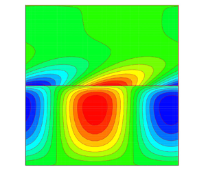
In order to validate the dominant mode of instability and understand the flow dynamics in terms of the streamfunction and temperature contours at the critical level, figures 12 and 13 are analysed. These secondary flow patterns are of the dominant mode of instability at the critical point as observed in §§ 3.1 and 3.2. Thus, the parameter values are kept the same as in § 3.2. In figures 12 and 13, (a–c) we present the streamfunction variation and in (d–f) the corresponding temperature contours. The vertical axis represents the porous domain extension from  $-1$ to 0 and the fluid domain extension from 0 to 1. The horizontal axis is the critical wavelength, which is scaled by
 $\hat {d}$ for the porous domain. Note that, to understand the convection patterns at the critical point more clearly, we have scaled the critical wavelength of the disturbance function in the porous domain such that the wavelength of the fluid domain is the same as the scaled wavelength of the porous domain. Furthermore, in the present study, the system is heated from below and
 $T_L>T_o>T_U$. Before the onset of convection, heat transfer takes place from the bottom to the top through conduction and sideways through fixed forced flow. Thus, in this situation, the fluid in the porous domain is lighter than the same in the fluid domain. As the temperature difference reaches a critical level in terms of the critical Rayleigh number, the heavier fluid tends to roll down and generates convection rolls. This marks the onset of convection in the system. In the present case, there are two factors that decide the flow patterns: one is the forced flow and the other the buoyancy force. The distribution of the streamfunction consists of alternatively clockwise (positive streamline) and counterclockwise (negative streamline) rotating convective cells.
The streamfunction patterns for (a)  $\hat {d}=0.1,\delta =0.001,Re=10,Pr=10,A=-1,$
 $\xi =0.001$, (b)
 $\hat {d}=0.13,\delta =0.0005,Re=10, Pr=10, A=0, \xi =0.1$ and (c)
 $\hat {d}=0.2,\delta =0.001,Re=10,Pr=10,A=-1,\xi =10$ with corresponding temperature profiles in (d–f). The contour legends are shown alternatively in the colour bar.

The streamfunction patterns for, (a)  $\hat {d}=0.1,\delta =0.001,Re=100,Pr=10,A=-1$,
 $\xi =0.001$, (b)
 $\hat {d}=0.1, \delta =0.001,Re=20, Pr=10, A=0, \xi =0.001$ and (c)
 $\hat {d}=0.1, \delta =0.001,Re=10, Pr=0.01, A=1, \xi =10$ with corresponding temperature profiles in (d–f). The contour legends are shown alternatively in the colour bar.

Figure 12(a) shows that the convection cells are confined to both fluid and porous domains with a comparatively dominant nature in the porous domain, which shows that the porous mode dominates the flow instability. The corresponding temperature contour presented in figure 12(d) shows the presence of convective cells in the entire porous domain, whereas, in the fluid domain, these are limited to the vicinity of the interface only. Thus, the role of the thermal–buoyant force in the porous domain in determining the flow instability is expected. Figure 12(b) shows that the onset of convection is mostly confined to the fluid domain with some flow penetration in the upper region of the porous domain. It is to be noted that, in comparison with the previous case, where the permeability along the vertical direction was 1000 times the permeability along the horizontal direction, here, the same is only 10 times. Due to this restrictive nature of the porous medium, the flow does not penetrate very far into the  $z_m$-direction. The temperature contour for this case (figure 12e) shows a distribution of convective cells limited to the fluid domain and indicates the thermal–buoyant instability in the fluid domain. A similar geometric feature is also shown in the streamfunction in figure 12(c) and the corresponding temperature contour in figure 12(f). In figure 12(c), a very small portion of the streamfunction penetrates into the porous domain due to the momentum diffusion effect induced by the fluid domain. The corresponding temperature contour reveals the spreading out of the convective cells in the entire fluid domain, implying instability in the fluid domain. The convective cells in the fluid domain illustrate a nearly square pattern for the streamfunctions whereas these are centro-symmetric about the horizontal axis for the isotherms (figure 12b–c,e–f). Figures 13(a) and 13(b) exhibit a similar pattern to figure 12(a), indicating that the porous mode is the dominant mode of instability, but the tilted convective cells show the impact of shear, i.e.
 $Re$ on the instability of the flow. The temperature profiles (figure 13d,e) show the distribution of convective cells in the lower part of the fluid domain, which indicates the impact of interface conditions over the flow dynamics in the inhomogeneous porous medium. The streamfunction variation in figure 13(c) is similar to that in figures 12(b) and 12(c), with a decrease in the values of the Prandtl number and depth ratio, representing the dominant instability by the fluid domain and a slight interfacial temperature disturbance in the porous domain (figure 13f).
On the whole, for the temperature contours, the role of the interface is significant when the instability is in the porous domain, whereas it is negligible for instability in the fluid domain. The streamfunctions are distributed in either the entire fluid and porous domains or occupy the fluid and upper region of the porous domain. Whereas the temperature contours either occupy the entire fluid and porous domains or occupy the porous and lower region of the fluid domain.
4. Conclusions
The current study delves into the thermal convection of a Newtonian fluid in an anisotropic and inhomogeneous porous domain underlying a fluid domain enforced with plane Poiseuille flow. A two-domain approach is adopted to execute a linear stability analysis of the superposed system separated by an interface. The present study is also well validated with the theoretical and experimental works of Sun (Reference Sun1973), Chen & Chen (Reference Chen and Chen1988), Chen & Chen (Reference Chen and Chen1989) and Chang (Reference Chang2006). Investigation of linear stability subjected to infinitesimal perturbations manifests the presence of the fluid mode, the porous mode and the bi-mode (both porous and fluid modes) via the neutral curve plots on the criticality of the Rayleigh number in the porous domain vs the wavenumber in the porous domain. The development of various modes is observed for various values of the depth ratio, medium permeability in terms of Darcy number, anisotropy, inhomogeneity, Reynolds number and Prandtl number. It is observed that the introduction of anisotropy and inhomogeneity causes qualitative as well as quantitative changes in the stability analysis of the present study. In contrast to the existing literature results on isotropic and homogeneous porous domain (Chang Reference Chang2006), the conclusions drawn out from the linear stability analysis of the present study show that an increase in the parameter value of the anisotropy and a decrease in the inhomogeneity as well as the Darcy number, follow the shift from unimodal (here, the porous mode) to bimodal (i.e. both porous and fluid modes). However, in general, increasing the value of the depth ratio follows the shift from unimodal (i.e. porous mode) to bimodal and then finally unimodal instability in terms of the fluid mode, which also depicts the interaction of the unstable modes along the interface. It is important to mention here that a trimodal instability is also observed for  $\hat {d}=0.2$,
 $\delta =0.001$,
 $\xi =0.001$,
 $0.1$, 1 and
 $A=0$,
 $1$. Also, a decrease in the value of the Reynolds number follows the shift from unimodal (here, the porous) to bimodal. The neutral curves for various Prandtl numbers demonstrate the porous mode for low anisotropy and both the porous and fluid modes for higher anisotropy. The neutral curves are independent with respect to a change in the Prandtl number for fixed values of the inhomogeneity. For a low magnitude of the anisotropy, Darcy number, Reynolds number and Prandtl number, and a large magnitude of the inhomogeneity and depth ratio under consideration, it is also noted that instability is obtained sooner, i.e. the critical Rayleigh number is small. The findings reached so far are based on the assumption that, when one parameter is changed, the others remain constant. Further, irrespective of the anisotropy and inhomogeneity under consideration, it is found that the least stable mode (dominant) is always porous for
 $\hat {d}<0.05$ and fluid for
 $\hat {d}>0.16$.
A look at the energy budget analysis aids in classifying the instabilities. The instability is found to be thermal–buoyant with the exception of thermal–shear instability for low Reynolds numbers with low anisotropy. The variation of streamlines and isotherms at the dominant mode of instability are analysed to understand the instability mechanism and also provide information regarding the secondary flow pattern. For the temperature contours, it is observed that the interface plays a significant role when the instability is in the porous domain and shows a negligible impact for instability in the fluid domain. Additionally, the energy budget and secondary flow patterns add value to the validation of the modes observed by the linear stability analysis.
It is anticipated that the present research will help to fathom the thermal convection of shear flows in such superposed systems. Likewise, an attempt towards the nonlinear stability analysis for such systems can be of great interest to gain possible clues regarding transition to turbulence in terms of bifurcation as well as secondary flow patterns in the transition regime. Furthermore, it is also possible that a short-time growth may occur in these types of superposed systems (Sengupta & De Reference Sengupta and De2019a). Thus, the transient amplifications can also be understood by the non-modal analysis. These analyses are left for our future studies.
Acknowledgements
One of the authors, P.B., dedicates this work to Professor V. Eswaran, Indian Institute of Technology Hyderabad, India, on his 63rd birth anniversary. The authors express gratitude to Professor Gaurav, Department of Chemical Engineering, Indian Institute of Technology Roorkee, for his valuable discussions. The authors also express their sincere indebtedness and gratitude towards the anonymous reviewers whose remarks considerably aided in the improvement of the article.
Funding
This work is partially supported by SERB, India (project grant no. EEQ/2020/000101 and MTR/2020/000187). One of the authors, Anjali., is grateful to the Ministry of Human Resource Development (MHRD), India for providing financial support during the preparation of this manuscript.
Declaration of interests
The authors report no conflict of interest.
Appendix A. A note on the considered model
The incorporation of a viscous diffusion term into Darcy's law, i.e. Brinkman's correction, remains argued in the literature. The most prominent findings in the literature related to the appropriate choice of model for a porous domain show the validity of the Brinkman model for a porous domain with high porosity (Nield Reference Nield1991; Auriault Reference Auriault2009; Hill & Straughan Reference Hill and Straughan2009b; Nield & Bejan Reference Nield and Bejan2013). If the porous medium is highly permeable and highly porous (i.e. porosity is  ${>}0.6$), the Brinkman model is recommended, which is due to the fact that the characteristic inter-pore distance in such systems is no longer insignificant compared with the characteristic length scale associated with volume averaging. As a result, during volume averaging, the viscous Laplacian terms for these systems become crucial and are retained. This results in the Brinkman terms as viscous corrections to the Darcy model (which can be safely ignored for low porosity, resulting in the Darcy model). However, if the flow strength is increased, an averaged model with inertial corrections, such as the Forchheimer equation, is expected to be valid and is welcomed.
In the present study, we are interested in understanding the flow instability for a small value of porosity. Accordingly, the chosen value of porosity in the manuscript is 0.3. Hence, the classical Darcy law is employed in the present study.
Appendix B. Non-dimensional basic velocities
We have
 $$\begin{gather} \bar{U}(z)=C_1z^{2}+C_2z+C_3, \quad 0\leqslant z \leqslant 1, \end{gather}$$
 $$\begin{gather}\overline{U_m}(z_m)=\frac{\eta_x(z_m)}{\eta_x(0)}, \quad -1 \leqslant z_m \leqslant 0, \end{gather}$$
where
 \begin{gather} C_1={-}\frac{4 \hat{d}^{2}}{F},\quad C_2= \frac{4 \hat{d} \alpha_{BJ}[\hat{d}^{2}-2 \delta^{2} \eta_x(0)]}{F [\delta \sqrt{\eta_x(0)}+\hat{d} \alpha_{BJ}]}, \end{gather}
 \begin{gather}C_3= \frac{4 \hat{d} \delta [2 \alpha_{BJ} \delta \eta_x(0) + \hat{d}\sqrt{\eta_x(0)}]}{F [\delta \sqrt{\eta_x(0)}+\hat{d} \alpha_{BJ}]}, \end{gather}
 \begin{gather}F= \frac{\alpha_{BJ}^{2}[\hat{d}^{2}-2 \delta^{2} \eta_x(0)]^{2}}{ [\delta \sqrt{\eta_x(0)}+\hat{d} \alpha_{BJ}]^{2}}+\frac{4 \hat{d} \delta [2 \alpha_{BJ} \delta \eta_x(0) + \hat{d}\sqrt{\eta_x(0)}]}{ [\delta \sqrt{\eta_x(0)}+\hat{d} \alpha_{BJ}]}. \end{gather}
Appendix C. Expressions in the KE balance
We have
 \begin{gather} KE=\frac{1}{2 \lambda}\int_{0}^{1} \int_{0}^{\lambda} (u^{2}+w^{2}) \,{\rm d}\kern 0.06em x \,{\rm d}z , \end{gather}
 \begin{gather}KE_m=\frac{1}{2 \lambda_m}\int_{{-}1}^{0} \int_{0}^{\lambda_m} (u_m^{2}+w_m^{2}) \,{\rm d}\kern 0.06em x_m \,{\rm d}z_m , \end{gather}
 \begin{gather}E_s={-}\frac{1}{\lambda}\int_{0}^{1} \int_{0}^{\lambda} uw \left(\frac{{\rm d}\bar{U}}{{\rm d}z}\right) {{\rm d}\kern 0.06em x} \,{\rm d}z , \end{gather}
 \begin{gather}E_b=\frac{Ra}{\lambda Re^{2}}\int_{0}^{1} \int_{0}^{\lambda} Tw \,{\rm d}\kern 0.06em x \,{\rm d}z , \end{gather}
 \begin{gather}E_d={-}\frac{1}{\lambda Re}\int_{0}^{1} \int_{0}^{\lambda} \left[2 \left(\frac{\partial u}{\partial x}\right)^{2}\!+\!\left(\frac{\partial u}{\partial z}\right)^{2} +\left(\frac{\partial w}{\partial x}\right)^{2}\!+\!2 \left(\frac{\partial u}{\partial z}\right) \left(\frac{\partial w}{\partial x}\right)\!+\! 2 \left(\frac{\partial w}{\partial z}\right)^{2} \right] {\rm d}\kern0.7pt x \,{\rm d}z , \end{gather}
 \begin{gather}I={-}\frac{1}{\lambda Re} \int_{0}^{\lambda} \left[2w\frac{\partial w}{\partial z}+u\frac{\partial u}{\partial z} +u\frac{\partial w}{\partial x} \right]_{z=0} \,{{\rm d}\kern 0.06em x} , \end{gather}
 \begin{gather}E_{bm}=\frac{1}{\lambda_m}\int_{{-}1}^{0} \int_{0}^{\lambda_m} \frac{\chi Ra_m T_m w_m}{\delta^{2} Re_m^{2}}\,{\rm d}\kern 0.06em x_m \,{\rm d}z_m , \end{gather}
 \begin{gather}E_{Dm}={-}\frac{1}{\lambda_m}\int_{{-}1}^{0} \int_{0}^{\lambda_m}\frac{\chi}{Re_m}\left[\frac{u_m^{2}}{\delta^{2} \eta_x(z_m)}+\frac{\xi w_m^{2}}{\delta^{2} \eta_z(z_m)} \right] {\rm d}\kern 0.06em x_m \,{\rm d}z_m . \end{gather}
Appendix D. The trimodal stability in case of  $\hat {d}=0.2$

The plots of oscillatory frequency and the energy curves are shown to demonstrate the trimodal nature of the instability in case of the parameters discussed in § 3.1. One such case is  $\hat {d}=0.2$,
 $\delta =0.001$,
 $\xi =0.1$,
 $A=1$,
 $Re=10$ and
 $Pr=10$ (see figure 14 of Appendix D). As can be seen from the neutral stability curve as well as the energy balance curve, that there are three modes in the system, first the fluid mode for
 $a_m<0.24$, then the porous mode for
 $0.25< a_m<1.8$ and then again the fluid mode for
 $a_m>1.8$, hence, we call it the trimodal instability.
Neutral and energy components for  $\hat {d}=0.2$,
 $\xi =0.1$,
 $A=1$,
 $Re=10$,
 $Pr=10$ and
 $\delta =0.001$.


 Open access

