


1. Introduction
The thermoelectric effect enables the conversion of thermal energy and electrical energy between conductive materials, finding applications across various fields (Zhao & Tan Reference Zhao and Tan2014). For instance, thermocouples, commonly employed for temperature measurement, operate as temperature sensors based on the thermoelectric effect. In some waste heat recovery devices, the thermoelectric effect is utilised to convert waste heat into electrical energy, enabling energy recycling (Pourkiaei et al. Reference Pourkiaei, Ahmadi, Sadeghzadeh, Moosavi, Pourfayaz, Chen, Pour Yazdi and Kumar2019). The underlying mechanism is the development of thermoelectric current
 $\boldsymbol{{J}}$
between two different conductive materials when a temperature gradient exists along their interface, leading to a modified form of Ohm’s law (Gorbunov Reference Gorbunov1988; Cramer, Zhang & Gerbeth Reference Cramer, Zhang and Gerbeth2009):
 \begin{align} \boldsymbol{{J}} = \sigma (\boldsymbol{{E}} -S\, \boldsymbol{\nabla} T), \end{align}
where
 $\sigma$
,
 $\boldsymbol{{E}}$
and
 $S$
are the electrical conductivity, electric field and thermoelectric coefficient of the material, and
 $\boldsymbol{\nabla} T$
denotes the interfacial temperature gradient. When the contacting materials exhibit fluidity and are subjected to an applied magnetic field – such as in the solidification processes within the metallurgical industry (Moreau et al. Reference Moreau, Laskar, Tanaka and Camel1993), lithium–lead flow within stainless steel conduits in the liquid blanket of nuclear fusion reactors (Chen et al. Reference Chen, Wang and Chen2022, Reference Chen, Xie, Yang and Ni2023b
), or the interaction between liquid iron and semiconducting silicates at the core-mantle boundary of planets in planetary geophysics (Inglis Reference Inglis1955) – the conventional form of thermoelectric current requires redefinition (Shercliff Reference Shercliff1979b
):
 \begin{align} \boldsymbol{{J}} = \sigma (\boldsymbol{{E}} + (\boldsymbol{{u}} \times \boldsymbol{{B}})-S\boldsymbol {\nabla} T). \end{align}
Here,
 $\boldsymbol{{u}}$
and
 $\boldsymbol{{B}}$
represents the velocity of the material and the external magnetic fields. When the applied magnetic field possesses a component perpendicular to the thermoelectric current, the resulting Lorentz force,
 $\boldsymbol{{J}}\times \boldsymbol{{B}}$
, induces fluid motion, giving rise to thermoelectric magnetohydrodynamics (TEMHD) convection (Shercliff Reference Shercliff1979a
,Reference Shercliff
b
).
Although the theoretical framework of TEMHD convection was established by Shercliff (Reference Shercliff1979a ,Reference Shercliff b ) as early as 1979, research on the thermoelectric effect in convective heat transfer and related fields remains limited. For instance, in fusion engineering where the liquid blanket is subjected to high temperature differences and strong magnetic fields, the thermoelectric effect is often overlooked, as it is generally considered to have a negligible impact compared to buoyancy effects (Jing, Ni & Wang Reference Jing, Ni and Wang2013; Zhu, Chen & Ni Reference Zhu, Chen and Ni2024). However, some experiments and theoretical studies have observed or predicted the significant influence of the thermoelectric effect. It has been confirmed experimentally that the thermoelectric effect can drive rapid rotation in liquid metals, with a comparison made to the Marangoni effect (Jaworski et al. Reference Jaworski, Gray, Antonelli, Kim, Lau, Lee, Neumann, Xu and Ruzic2010). Within fusion divertor research as well, the thermoelectric effect is regarded as a highly effective means of cooling the blanket structure (Kaita et al. Reference Kaita2007; Horacek et al. Reference Horacek2018). In Rayleigh–Bénard (RB) experiments, the impact of the thermoelectric effect on the large-scale circulation of RB convection has also been predicted and observed (Kurenkova, Zienicke & Thess Reference Kurenkova, Zienicke and Thess2001; Xu, Horn & Aurnou Reference Xu, Horn and Aurnou2022). Except on the solid–liquid interface, thermoelectric driving has been observed experimentally between layered fluids (Vernet, Fauve & Gissinger Reference Vernet, Fauve and Gissinger2024). In summary, within fusion research, the thermoelectric effect cannot be entirely disregarded. However, the conditions under which it should be considered, as well as the methods for its inclusion, remain insufficiently studied, necessitating urgent, systematic investigation.
The thermoelectric effect influences convection through two opposing mechanisms. On one hand, the Lorentz force induced by the thermoelectric current drives the flow, with its direction dictated by the magnetic field orientation. On the other hand, the flow driven by the thermoelectric current is inherently limited. Once the magnetic field strength exceeds a critical threshold, the intensified magnetic damping effect suppresses the flow.
The present study demonstrates the significant role of the thermoelectric effect in vertical convection (VC) by ingeniously designing the magnetic field distribution to enhance heat transfer efficiency. It also theoretically derives the influence of the thermoelectric effect on convective heat transfer, and identifies key influencing parameters of the thermoelectric effect. In the following text, we will collectively refer to the issues that we are studying as thermoelectric VC (TEVC). Moreover, this method of improving heat efficiency differs from traditional means used in RB convection, such as rough walls (Shen, Tong & Xia Reference Shen, Tong and Xia1996; Xie & Xia Reference Xie and Xia2017; Jiang et al. Reference Jiang, Zhu, Mathai, Verzicco, Lohse and Sun2018, Reference Jiang, Zhu, Mathai, Yang, Verzicco, Lohse and Sun2019), geometric constraints (Huang et al. Reference Huang, Kaczorowski, Ni and Xia2013; Chong et al. Reference Chong, Huang, Kaczorowski and Xia2015; Chen et al. Reference Chen, Xie, Yang and Ni2023a
) and the multiphase flow approach (Yang et al. Reference Yang, Chong, Wang, Verzicco, Shishkina and Lohse2020; Liu et al. Reference Liu, Chong, Ng, Verzicco and Lohse2022; Chong et al. Reference Chong, Qiao, Wu and Wang2024). Instead, this research focuses primarily on the interaction of currents generated by the thermoelectric effect with an applied magnetic field, resulting in Lorentz forces that produce moments to either enhance or suppress the strength of large-scale circulation, thereby improving or inhibiting heat transfer efficiency. Compared to traditional heat transfer enhancement methods, the thermoelectric effect provides greater control over heat transfer by adjusting the intensity of the applied magnetic field, enabling precise modulation of heat transfer efficiency within a specific range. This capability has significant implications for advancing liquid metal cooling technologies, including enhancing the cooling efficiency of liquid metals used in electronic components for high-performance servers (Ma & Liu Reference Ma and Liu2007a
,Reference Ma and Liu
b
). After packaging, chip dimensions are generally of the order of several centimetres, depending on the application. For instance, a surface heat source measuring
 $5.6 \ \textrm{cm}\times 5.2 \ \textrm{cm}$
has been used to model the thermal load of a Pentium-IV CPU (Li et al. Reference Li, Lv, Liu and Zhou2006). The realisation of liquid metal flow driving for thermal management within spatial domains of only a few centimetres has been the subject of extensive investigation. Various driving mechanisms have been proposed for liquid metal cooling in microelectronic devices, including magnetohydrodynamic (MHD) pumps (Liu et al. Reference Liu, Zhou, Lv and Li2005), peristaltic pumps (Li et al. Reference Li, Lv, Liu and Zhou2006) and electro-wetting-based pumps (Mohseni Reference Mohseni2005). These methods typically require complex circuitry and auxiliary energy input, often resulting in bulky and intricate cooling systems. In contrast, convection induced by thermoelectric effects in conjunction with a non-uniform magnetic field offers the possibility of a self-contained driving mechanism within a sealed vessel, presenting a novel approach to liquid metal cooling.
The paper is organised as follows. Section 2 offers an overview of the physical model and numerical algorithms used in the present simulations. Section 3 presents the study’s results, starting with an analysis of heat and momentum transport in TEVC (§ 3.1), followed by an examination of heat transfer enhancement mechanisms (§ 3.2). Subsection 3.3 categorises the potential flow patterns, while § 3.4 develops a physical model for the TEVC phenomenon, supported by theoretical analysis. Finally, Section 4 concludes with a summary of the main findings.
2. Problem statement and formulation
We examine the flow of liquid lithium within a stainless steel enclosure subjected to a linearly varying horizontal magnetic field, as depicted in figure 1. The liquid lithium is assumed to be an incompressible, Newtonian viscous fluid under the Oberbeck–Boussinesq approximation. The computational domain for the fluid is defined as
 $[-L/2, L/2] \times [-L/2, L/2] \times [-L/2, L/2]$
, and the stainless steel shell has thickness d. As illustrated in figure 1(b,c), the device is situated within linear magnetic fields, given by
 $\boldsymbol{{B}}=(2B_0/L)x\boldsymbol{{k}}$
, where
 $\boldsymbol{{k}}$
denotes the unit vector in the
 $z$
-direction. Notably, although this magnetic field distribution is relatively idealised, it closely resembles the magnetic field distribution in the intermediate region between two infinitely long wires carrying currents in the same direction. When the direction of the current is reversed, the direction of the magnetic field will also be reversed.
(a) A sketch of a convection cell covered by stainless steel. (b,c) Two types of linear magnetic field distributions in the
 $x{-}z$
plane.

For liquid lithium, the governing equations of thermolelectric magnetoconvection are as follows:
 \begin{align} &\boldsymbol{\nabla}\boldsymbol{\cdot}\boldsymbol{u}= 0, \end{align}
 \begin{align} & \frac {\partial \boldsymbol{{u}}}{\partial t} + (\boldsymbol{u \cdot \nabla} ) \boldsymbol{{u}} = - \frac {1}{\rho _f}\boldsymbol {\nabla} p + \nu (\boldsymbol{\nabla} ^2 \boldsymbol{{u}}) + \frac {1}{\rho _f}(\boldsymbol{{J}} \times \boldsymbol{{B}}) + \alpha _T T\boldsymbol{{g}}, \end{align}
 \begin{align} & \rho _f c_{pf}\frac {\partial T}{\partial t} + \boldsymbol{u \cdot \nabla} T = \lambda _f\, \boldsymbol{\nabla} ^2 T, \end{align}
 \begin{align} & \boldsymbol{{J}} = \sigma _f (- \boldsymbol{\nabla} \phi + (\boldsymbol{{u}} \times \boldsymbol{{B}})-S_f\boldsymbol {\nabla} T), \end{align}
 \begin{align} & \boldsymbol{\nabla} ^2 \phi = \boldsymbol{\nabla}\,{\boldsymbol{\cdot}}\,(\boldsymbol{{u}} \times \boldsymbol{{B}}-S_f\boldsymbol {\nabla} T). \end{align}
In the stainless steel, the governing equations for temperature and electric potential are as follows:
 \begin{align} &\rho c_{ps}\frac {\partial T}{\partial t} = \lambda _s\, \boldsymbol{\nabla} ^2 T, \end{align}
 \begin{align} &\boldsymbol{{J}} = \sigma _s(-\boldsymbol{\nabla} \phi - S_s\boldsymbol{\nabla} T), \end{align}
 \begin{align} &\boldsymbol{\nabla} ^2\phi = \boldsymbol{\nabla}\,{\boldsymbol{\cdot}}\,(-S_s\boldsymbol{\nabla} T). \end{align}
Here,
 $p$
,
 $\textit {u}$
,
 $\phi$
,
 $\textit {B}$
and
 $T$
are the fields of pressure, velocity, electric potential, magnetic and temperature deviation from a reference state, respectively. The parameters
 $\nu$
,
 $\alpha _T$
,
 $\rho$
,
 $c_p$
,
 $\lambda$
,
 $\sigma$
and
 $S$
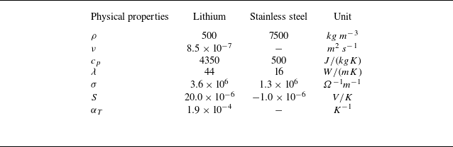
denote the kinematic viscosity, temperature expansion coefficient, density, heat capacity, thermal conductivity, electrical conductivity and thermoelectric coefficient. The subscripts f and s distinguish the properties of liquid lithium and stainless steel, respectively, with their specific values provided in table 1.
Physical properties of liquid lithium and stainless steel (Chen et al. Reference Chen, Xie, Yang and Ni2023b ).

No-slip boundary conditions are imposed on the fluid–solid interfaces, with
 $\boldsymbol{{u}}=0$
. Constant temperatures are maintained at the end faces:
 $T=T_h$
on the right-hand solid wall, and
 $T=T_c$
on the left, while an adiabatic boundary condition is set on the remaining solid wall. At the fluid–solid interface, continuity of temperature, heat flux, electric potential and the normal component of electric current is enforced.
In TEMHD convection, apart from the three traditional dimensionless parameters in MHD thermal convection – namely, the Rayleigh number (
 $Ra$
), Prandtl number (
 $Pr$
) and Hartmann number (
 $Ha$
), defined as
 \begin{align} Ra=\frac {\alpha _T g L^3\Delta T }{ \nu \kappa }, \quad Pr = \frac {\nu }{\kappa } , \quad Ha=B_0L\sqrt {\frac {\sigma _f}{\rho _f \nu }} \end{align}
– there are two additional parameters: the thermoelectric number (
 $Te$
), which represents the strength of the thermoelectric effect, and the fluid–solid conductivity ratio (
 $C_w$
), defined as
 \begin{align} Te=\frac {\sigma _f\Delta SB_0\Delta TL^2}{\rho _f\nu ^2}, \quad C_w=\frac {\sigma _sd }{ \sigma _f L}. \end{align}
Here,
 $\Delta T=T_h-T_c$
is the temperature difference between the left- and right-hand solid walls,
 $\Delta S$
is the Seebeck coefficient difference between the liquid and solid,
 $d$
is the thickness of the solid wall, and
 $L$
is the fluid domain length. We select the maximum magnetic field strength in the fluid region as the characteristic magnetic field strength
 $B_0$
. The response parameters are the Nusselt number and Reynolds number:
 \begin{align} Nu=QL / \kappa _f\,\Delta T, \quad Re=UL / \nu , \end{align}
where
 $\kappa _f=\lambda _f / \rho _f c_{pf}$
is the thermal diffusivity,
 $Q$
is the heat flux crossing the fluid, and
 $U$
is the characteristic velocity of the flow.
The MHD solver MHD-UCAS (Ni et al. Reference Ni, Munipalli, Huang, Morley and Abdou2007a
,Reference Ni, Munipalli, Morley, Huang and Abdou
b
) based on the finite volume method, with second-order accuracy in both time and space, is employed to solve this problem, which has been validated in previous fluid–structure coupling problems and Seebeck effect problems (Chen et al. Reference Chen, Wang and Chen2022, 2023; Zhu et al. Reference Zhu, Chen and Ni2024b
). In this simulation study,
 $Ra$
is fixed at
 $10^5$
, and containers of different geometric sizes are simulated under various non-uniform magnetic fields. Given that
 $Ra \propto L^3$
and
 $Te \propto L^2$
, similar to the Marangoni effect, the geometric size determines the relative influence of the thermoelectric effect and buoyancy. For this study, considering all parameters as real physical values, the corresponding container sizes
 $L$
are set to
 $0.04$
,
 $0.05$
,
 $0.06$
and
 $0.08\ \text{m}$
, with solid wall thickness
 $L/40$
.
In addition to the internal flow structure, four boundary layers must be accurately resolved (Grossmann & Lohse Reference Grossmann and Lohse2000; Davidson Reference Davidson2002): the thermal boundary layer
 $\delta _T \approx 1/(2\,Nu)$
, the viscous boundary layer
 $\delta _{\nu } \approx 1/(4\,\sqrt {Re})$
, the Shercliff layer
 $\delta _{Sh} \approx 1/\sqrt {Ha}$
, and the Hartmann layer
 $\delta _{Ha} \approx 1/Ha$
. To achieve this, a coordinate transformation is used to generate a non-uniform grid (Akhmedagaev et al. Reference Akhmedagaev, Zikanov, Krasnov and Schumacher2020).
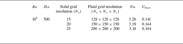
To verify grid resolution, a grid convergence study for TEVC is conducted in Set-A (see figure 1) at
 $Ha = 500$
and
 $L = 0.04\ \text{m}$
, as listed in table 2. Three grid resolutions are tested, yielding
 $Nu$
values
 $3.26$
,
 $3.19$
and
 $3.18$
, and
 $U_{max}\ $
values
 $0.141$
,
 $0.144$
and
 $0.144$
. The second grid is selected as the computational grid, providing a reasonable basis for numerical simulation. We report statistics averaged over at least
 $400$
dimensionless turnover times (Stevens, Verzicco & Lohse Reference Stevens, Verzicco and Lohse2010), where a turnover time is defined as the free-fall period
 $H / U_{\Delta T}$
, with
 $U_{\Delta T} = (g \beta\, \Delta T\, H)^{1/2}$
.
Grid resolution studies for TEVC at
 $Ra=10^5$
,
 $Ha=500$
and
 $L=0.04\,\textrm m$
.

3. Results and discussion
3.1. Global heat transfer and fluid structure
We commence by exploring the impact of varying magnetic field strengths on the heat transfer efficiency of the TEVC under two distinct magnetic field configurations, as illustrated in figures 2(a) and 2(d). These visualisations detail the variations in heat transfer efficiency across four selected devices subjected to the magnetic field distributions designated as Set-A and Set-B. To elucidate the enhancement in
 $Nu$
, the data have been normalised using
 $Nu_0$
, corresponding to the baseline case at
 $Ha = 0$
, while
 $Ha$
is systematically varied within the range
 $10$
–
 $1000$
. In the present work,
 $Nu_0$
remains approximately constant at
 $2.2\ (\pm 1.3\,\%)$
across different geometric scales. This consistency arises from the fact that in the absence of a magnetic field, all four device sizes share identical non-dimensional parameters – including the Rayleigh number (
 $Ra$
), the fluid–solid thickness ratio (
 $d/L$
), and all material properties. This invariance enables a quantitative assessment of heat transfer enhancement across geometries via the normalised Nusselt number.
The results reveal consistent trends in
 $Nu$
across the four container devices. In Set-A,
 $Nu$
exhibits an initial increase with rising
 $Ha$
, reaching a peak before subsequently declining. Remarkably, for the smallest device, with
 $L = 0.04\text{ m}$
, the maximum enhancement in heat transfer efficiency nears 60
 $\,\%$
, occurring at approximately
 $Ha = 300$
. Beyond this threshold, as
 $Ha$
continues to increase,
 $Nu$
steadily diminishes. The amplitude of
 $Nu$
variation lessens with larger
 $L$
, leading to reduced heat transfer efficiency at equivalent
 $Ha$
values. For the largest device,
 $L = 0.08\text{ m}$
, the peak enhancement in
 $Nu$
is limited to approximately 20
 $\,\%$
. It is important to note that as the Rayleigh number (
 $Ra$
) in this study is fixed, an increase in the characteristic length inevitably weakens the temperature gradient. This reduction diminishes the thermoelectric current and the resulting Lorentz force, thereby lessening their impact on flow and heat transfer.
In contrast, the behaviour of
 $Nu$
in Set-B diverges significantly from that of Set-A, as the TEVC performance here is influenced by the magnetic field polarity. In Set-B, the heat transfer efficiency undergoes a three-phase variation (see figure 2
d): an initial decrease, followed by an increase, and culminating in another decline as
 $Ha$
rises. This sequence encompasses both enhancement and suppression phases of heat transfer efficiency. At low
 $Ha$
, a rapid suppression of heat transfer is evident. Subsequently,
 $Nu$
begins to rise, and for smaller devices, such as those with
 $L = 0.04$
and
 $0.06\text{ m}$
, it can exceed
 $Nu_0$
. However, as the characteristic length
 $L$
increases,
 $Nu$
no longer surpasses
 $Nu_0$
.
(a,d) Plots of
 $Nu$
as functions of
 $Ha$
in different fluid regime sizes for Set-A and Set-B. (b,e) Plots of
 $Re$
as functions of
 $Ha$
in different fluid regime sizes for Set-A and Set-B. (c, f) Plots of
 ${Lm}_z$
as functions of
 $Ha$
in different fluid regime sizes for Set-A and Set-B.

To elucidate the underlying physical mechanisms behind the markedly different trends in
 $Nu$
, we computed the Reynolds number
 $Re$
. The characteristic velocity used for this calculation is defined as (Shishkina Reference Shishkina2016)
 \begin{align} U_m = {\max_{x}}A^{-1}\iint _{0}^{A}U_y{\textrm d}a. \end{align}
Here,
 $A$
represents the vertical plane perpendicular to the temperature gradient. Additionally, we calculated the global angular momentum (Zhang et al. Reference Zhang, Chen, Xia, Xi, Zhou and Chen2021; Hu, Zhang & Xia Reference Hu, Zhang and Xia2024). Given the fixed convection direction of the VC, and the alignment of the magnetic field along the
 $z$
axis, the Lorentz force is confined to the circulation plane. Consequently, we focus on the angular momentum in the circulation direction, expressed as
 $Lm_z = \langle yu_x - xu_y \rangle$
. As shown in figure 2(b,e), the
 $Re$
trend as a function of
 $Ha$
is generally consistent with the
 $Nu$
trend across both Set-A and Set-B. The distribution of extrema in the
 $Re$
variation curve corresponds closely with that of the
 $Nu$
curve, indicating that the magnetic field influences convection intensity, thereby affecting heat transfer efficiency. Furthermore, examining the angular momentum variation reveals an intriguing phenomenon in Set-B: as
 $Ha$
increases,
 $Lm_z$
transitions from positive to negative. This behaviour contrasts sharply with traditional VC (Shishkina Reference Shishkina2016; Wang et al. Reference Wang, Liu, Verzicco, Shishkina and Lohse2021), where fluid typically ascends near the hot wall, while fluid descends near the cold wall, a characteristic distinct from RB convection, which maintains a consistent flow direction. The sign change in
 $Lm_z$
indicate a flow reversal in VC.
This insight helps to clarify the mechanism underlying the observed behaviour in Set-B, where heat and momentum transport intensity first decrease, then increase. As
 $Ha$
rises from
 $0$
to the critical value marking the TEVC reversal, the Lorentz force suppresses the convection, reducing the initial convective strength and disrupting the large-scale circulation until the angular momentum along the
 $z$
axis approaches zero. At this point, the large-scale circulation ceases, resulting in minimal heat and momentum transport. Subsequently, as the magnetic field further intensifies, the TEVC reversal occurs, enabling large-scale circulation to re-establish and enhancing both heat and momentum transport. However,
 $Nu$
does not necessarily increase monotonically with the strength of the magnetic field. At sufficiently high
 $Ha$
, magnetic damping becomes dominant, leading to a suppression of convective transport, as will be discussed in detail below.
As the angular momentum in the
 $z$
-direction transitions from positive to negative, signalling a reversal of the TEVC, the internal flow structure within the container warrants further investigation. The objective is to determine whether this phenomenon merely suppresses convection or leads to the fragmentation of large-scale circulation and the formation of multiple vortices. To analyse the TEVC flow structure, the variations of vertical velocity
 $\langle \bar {U}_y \rangle _{y,z}$
and temperature
 $\langle \bar {T} \rangle$
along the
 $x$
axis are presented for
 $L = 0.05\text{ m}$
, as depicted in figure 3(a,b). The distribution curves exhibit approximate antisymmetry about
 $x = 0.025$
, with selected characteristic
 $Ha$
values highlighted for clarity.
(a) Time-averaged vertical velocity
 $\langle \bar {U}_y \rangle _{yz}$
profiles at
 $(x/L,y/L)=(0.5,0.5)$
with
 $Ra=10^5$
for cases of Set-A and Set-B. (b) Time-averaged temperature
 $\langle \bar {T}\rangle _{yz}$
profiles at
 $(x/L,y/L)=(0.5,0.5)$
with
 $Ra=10^5$
for cases of Set-A and Set-B. The solid lines correspond to Set-A cases, and the dotted lines correspond to Set-B cases. Time-averaged
 $u_y$
fields and streamlines at
 $L=0.05\ \text{m}$
and (c) Set-B,
 $Ha=500$
, (d) Set-B,
 $Ha=30$
, (e)
 $Ha=0$
, (f) Set-A,
 $Ha=500$
.

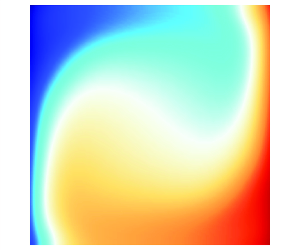
For Set-A, the curve distribution mirrors that of traditional VC, where the fluid near the hot wall ascends, and convective intensity is amplified under the influence of the magnetic field. Figure 3(c–f) show the
 $y$
-direction velocity contours and streamlines as the field transitions from Set-B to Set-A. Figure 3(e) illustrates VC flow in the absence of a magnetic field, displaying the characteristic rising fluid near the hot wall and descending fluid near the cold wall – an archetypal convection structure. As seen in figure 3(c), under a strong magnetic field in Set-B (
 $Ha = 500$
), large-scale circulation forms in opposition to traditional VC. The convection intensity is significantly higher than that in VC, as shown in figure 3(a), while the flow intensity in the bulk remains relatively weak. In Set-B at
 $Ha = 30$
(figure 3
a,b,d), the flow weakens further, and the cavity develops multiple vortices, with large-scale circulation absent, and temperature distribution approaching conductive heat transfer. In contrast, under Set-A’s strong magnetic field (
 $Ha = 500$
), as shown in figure 3(f), the circulation direction aligns with that of VC. The convection intensity exceeds that of VC, yet remains concentrated near the walls, with significantly stronger convection at the walls compared to the bulk flow.
3.2. Mechanism of heat transfer enhancement
According to the study of the RB reversal problem (Zhang et al. Reference Zhang, Chen, Xia, Xi, Zhou and Chen2021; Hu et al. Reference Hu, Zhang and Xia2024), the angular momentum equation is expressed as
 \begin{align} \frac{{\textrm d}\boldsymbol{{L}}_m}{{\textrm d}t} &= -\langle \boldsymbol{{r}} \times (\boldsymbol{{u}}\cdot \boldsymbol{\nabla} \boldsymbol{{u}})\rangle - \langle \boldsymbol{{r}} \times \boldsymbol{\nabla} p_0 \rangle + \sqrt {\frac {Pr}{Ra}}\langle \boldsymbol{{r}} \times \boldsymbol{\nabla} ^2\boldsymbol{{u}}\rangle + \langle \underbrace {\boldsymbol{{r}}\times (T \boldsymbol{{j}}-\boldsymbol{\nabla} p_{t})\rangle }_{\sigma _{Buo}} \notag \nonumber \\ &\quad+\, \underbrace {Ha^2\sqrt {\frac {Pr}{Ra}}\langle \boldsymbol{{r}} \times ((-\boldsymbol{\nabla} \phi _{md}+\boldsymbol{{u}}\times B\boldsymbol{{k}})\times B\boldsymbol{{k}})\rangle }_{\sigma _{MD}} \nonumber \\ &\quad +\, \underbrace {Ha^2\,Se\,\sqrt {\frac {Pr}{Ra}}\langle \boldsymbol{{r}}\times ((\boldsymbol{\nabla} T -\boldsymbol{\nabla} \phi _{te})\times B\boldsymbol{{k}})\rangle }_{\sigma _{TE}}, \end{align}
where
 $\boldsymbol{{L}}_m=\langle \boldsymbol{{r}} \times \boldsymbol{{u}} \rangle$
represents the global angular momentum. The final three items on the right-hand side of (3.2) correspond the buoyancy angular momentum moment, the MHD damping angular momentum moment, and the thermoelectric angular momentum moment, respectively. Here,
 $\langle \cdot \rangle _x$
,
 $\langle \cdot \rangle _y$
,
 $\langle \cdot \rangle _z$
and
 $\langle \cdot \rangle$
denote averaging along the
 $x$
axis, the
 $y$
axis, the
 $z$
axis, and over the entire fluid volume. The variable
 $p_t$
is the buoyancy-induced pressure, with governing equation and boundary condition
 \begin{align} \boldsymbol{\nabla} ^2p_t=\partial T / \partial y, \quad \partial p_t/\partial n = T\boldsymbol{{j}}\cdot \boldsymbol{{n}}. \end{align}
Above,
 $T \boldsymbol{{j}}-\boldsymbol{\nabla} p_{t}$
is the divergence-free projection of the buoyancy force, and it corresponds to the net contribution of the temperature field to the velocity fields (Zhang et al. Reference Zhang, Chen, Xia, Xi, Zhou and Chen2021; Hu et al. Reference Hu, Zhang and Xia2024). Here, the electric potential
 $\boldsymbol{\nabla} \phi$
is decomposed into two components:
 $\boldsymbol{\nabla} \phi _m$
and
 $\boldsymbol{\nabla} \phi _{te}$
. The term
 $\boldsymbol{\nabla} \phi _m$
arises from the interaction between the magnetic induction and the moving liquid metal, while
 $\boldsymbol{\nabla} \phi _{te}$
is generated by the thermoelectric effect. Distinguishing the magnetic damping force from the thermal electromotive force within the Lorentz force is challenging in practice, and calculating the precise magnetic damping torque and thermoelectric torque is even more complex. Therefore, in the ongoing research, we will also examine the Lorentz force torque, denoted as
 $\sigma _{Luo}$
. Furthermore, the Lorentz force can be similarly treated to the approach applied to the buoyancy force discussed earlier:
 \begin{align} \boldsymbol{\nabla}\,{\boldsymbol{\cdot}}\,\boldsymbol{{F}}_{Luo}=\boldsymbol{\nabla} ^2 p_{J}, \quad \partial p_J/\partial n = \boldsymbol{{F}}_{Luo}\cdot \boldsymbol{{n}}. \end{align}
Following this formulation,
 $\boldsymbol{{F}}_{Luo}^{*}=\boldsymbol{{F}}_{Luo}-\boldsymbol{\nabla} p_J$
represents the net contribution of the Lorentz force to the velocity field, and the net Lorentz force torque
 $\sigma _{Luo}$
can be expressed as
 $\langle \boldsymbol{{r}}\times (\boldsymbol{{F}}_{Luo}-\boldsymbol{\nabla} p_J) \rangle$
. Subsequently, these resultant angular momentum torques will be employed to elucidate the underlying mechanisms governing heat and momentum transport variations.
From (3.2),
 $\sigma _{MD} \sim u B^2$
indicates that
 $\sigma _{MD}$
exhibits quadratic dependence on
 $B^2$
. Theoretically, changing the magnetic field’s polarity does not alter the direction of
 $\sigma _{MD}$
. However, for the thermoelectric angular momentum torque, the relation
 $\sigma _{TE} \sim \Delta \textit{TB}$
implies that a polarity reversal in the magnetic field will consequently invert the direction of
 $\sigma _{TE}$
. Additionally, as the temperature gradient is orthogonal to the magnetic field, a net electric current flows along the temperature gradient. In the lithium–stainless steel system, which forms a closed circuit, the Lorentz force generated by the thermoelectric current under the linear magnetic field induces thermoelectric-driven convection within the same plane as the large-scale circulation.
Through modulation of the magnetic field strength, we can precisely control both the magnitude and direction of the thermoelectric torque, thereby enabling regulated manipulation of VC heat transfer and flow characteristics. While the linear magnetic field represents one specific configuration, other non-uniform magnetic field geometries, including semi-space fields, gradient fields, and step fields, may similarly enable comparable control mechanisms. Here, an idealised model is presented, suggesting that with suitable non-uniform magnetic field design and distribution, more efficient configurations may exist for achieving controllable regulation of thermoconvection in liquid metals.
In figure 4(a,b), we present the heat and momentum transport in a device with
 $L=0.04\,\textrm m$
under a linear magnetic field, comparing scenarios of pure buoyancy-driven (PBD) and pure thermoelectric-driven (PTED) convection. Here, we use
 $Ha^*=\text{sgn}(\sigma _{Buo}\times \sigma _{TE})\,Ha$
to depict the transition from Set-A to Set-B magnetic field configurations, where the
 $\text{sgn}(\cdot )$
function denotes the sign of the values.
(a) Plot of
 $Nu$
as a function in PBD (
 $Te=0$
) and PTED (
 $Ra=0$
) convection of
 $Ha$
under Set-A and Set-B magnetic fields. (b) Plot of
 $Re$
as a function in PBD (
 $Te=0$
) and PTED (
 $Ra=0$
) convection of
 $Ha$
under Set-A and Set-B magnetic fields. The distribution of time-averaged temperature and
 $F^*_{Luo}$
vectors on the
 $z/L=0.5$
plane at
 $Ha=100$
and (c) Set-A, PBD, (d) Set-B, PBD, (e) Set-A, PTED, and (f) Set-B, PTED.

In the case of PBD convection, the thermoelectric coefficients
 $S$
of both lithium and stainless steel are artificially set to
 $0$
, thereby completely suppressing any thermoelectric effects. This configuration results in standard VC under a non-uniform magnetic field. As shown in figure 4(a,b), the heat transfer efficiency and momentum transport efficiency vary with increasing magnetic field strength. The two sides of
 $ Ha^* = 0$
correspond to the two distinct magnetic field distributions described earlier. As the magnetic field strength increases, both heat transfer efficiency and convection strength diminish, and this trend remains consistent regardless of the specific magnetic field configuration. Additionally, figure 4(e,f) reveal that the temperature distribution and
 $F^*_{Luo}$
vectors remain consistent across both magnetic field settings, and
 $F^*_{Luo}$
hinders thermal convection in both cases, indicating that PBD convection is independent of the magnetic field’s polarity.
For PTED convection without gravity, the behaviour of heat transfer efficiency and momentum transport as a function of
 $Ha$
diverges entirely from that of PBD convection. Under both magnetic field settings, these efficiencies increase with the strength of the magnetic field. However, beyond a certain threshold of
 $Ha$
, both
 $Nu$
and
 $Re$
start to decrease as
 $Ha$
continues to rise. Figures 4(c) and 4(d) demonstrate that the two magnetic field configurations induce opposite circulation directions for thermoelectric-driven flow, indicating that convection direction is contingent upon the magnetic field’s polarity. Consequently,
 $\boldsymbol{F}^*_{Luo}$
aligns with the flow direction and shifts in response to the magnetic field’s polarity. This observation suggests the potential to regulate convection direction through strategic manipulation of the magnetic field orientation.
For both PTED and TEVC systems, regardless of Set-A or Set-B configurations, when the applied magnetic field strength increases beyond a critical value, both heat transport and momentum transport undergo suppression. At this point,
 $\sigma _{MD}$
plays a dominant role. Across the various container geometries, a reversal phenomenon consistently arises: when the magnetic field is intensified to a certain extent, the thermoelectric effect takes precedence in controlling the flow. When the magnetic field is increased to a certain extent, the primary control factor for the flow will be the thermoelectric effect. Further increasing the magnetic field leads to a suppression of heat transfer and flow, driven primarily by the relative magnitudes of the thermoelectric torque
 $\sigma _{TE}$
and the magnetic damping torque
 $\sigma _{MD}$
. Notably,
 $\sigma _{MD}$
acts in the opposite direction to
 $\sigma _{TE}$
, with
 $\sigma _{MD} \sim -u B^2$
, inherently opposing the velocity, while
 $\sigma _{TE} \sim \Delta S\, \Delta T\, B$
. Under fixed temperature gradients, as the magnetic field strength increases, the rise in
 $\sigma _{MD}$
eventually surpasses that of
 $\sigma _{TE}$
at higher
 $Ha$
values, intensifying the suppressive effect of
 $\sigma _{MD}$
. In figure 6, we analyse data from the
 $L=0.08$
m device, calculating the net buoyancy torque and net Lorentz torque across different magnetic fields. This analysis clarifies why the heat transfer efficiency varies as depicted in figure 2(a,b). During flow reversal,
 $\sigma _{Buo} + \sigma _{Luo}$
transitions from positive to negative. In both Set-A and Set-B, as the magnetic field further increases,
 $\sigma _{Luo}$
begins to decrease, and consequently
 $\sigma _{Buo} + \sigma _{Luo}$
also diminishes, correlating with the observed attenuation in heat and momentum transport.
(a) Flow regimes in the
 $(L,Ha^*)$
parameter domain. The symbol ‘
 $+$
’ denotes regions where
 $\partial Re^*/\partial Ha^*\gt 0$
, while ‘
 $ -$
’ indicates
 $\partial Re^*/\partial Ha^*\lt 0$
. Here, the modified Reynolds numbers are defined as
 $Re^*=\text{sgn}(Lm_z)\,Re$
. (b) Plots of
 $Nu$
and
 $Re^*$
versus
 $Ha^*$
at
 $L=0.05\text{ m}$
. The dashed line represents the condition
 $Re^*=0$
. The distribution of time-averaged temperature and
 $F^*_{Luo}$
vectors on the
 $z/L=0.5$
plane at
 $L=0.05\text{ m}$
and (c) Set-B,
 $Ha=1000$
, (d) Set-B,
 $Ha=50$
, (e) Set-A,
 $Ha=50$
, (f) Set-A,
 $Ha=1000$
.

3.3. Flow regime of TEVC
Based on the previous analysis, for the lithium–stainless steel system under the parameters, three distinct flow regimes are observed in TEVC, which are preliminarily classified in figure 5(a). The formation of these regimes is predominantly influenced by the competing torques
 $\sigma _{Buo}$
,
 $\sigma _{TE}$
and
 $\sigma _{MD}$
. Under the influence of the magnetic field, both
 $\sigma _{TE}$
and
 $\sigma _{MD}$
vary, following significantly different trends. This variation generates Lorentz moments with distinct spatial distributions and effects depending on the magnetic field configuration. According to (3.4), the distribution of the modified Lorentz force
 $\boldsymbol{F}_{Luo}^{*}$
is illustrated in figure 5(c–f). Below, we summarise the variations in heat transfer, momentum transport, angular momentum, and flow structure characteristic of each flow regime.
-
I. Buoyancy-dominated regime. As depicted in figure 5(e), in this flow state, the direction of large-scale circulation coincides with that of VC. Under the Set-A magnetic field configuration, an increase in magnetic field strength elevates convective intensity, thereby enhancing heat transfer efficiency, with the magnetic damping effect proving insufficient to curb the flow. In contrast, in the Set-B magnetic field configuration, the thermoelectric angular momentum opposes the buoyancy-driven angular momentum; as magnetic field strength rises, the thermoelectric force suppresses thermal convection, leading to a reduction in heat transfer efficiency, although the convection direction remains stable. During the transition from Set-B to Set-A, as shown in figure 5(b), heat transfer efficiency increases monotonically as
 $Ha^*$
rises from the critical
$Ha$
value, where reversal occurs, to the point at which magnetic damping dominates. This range of the
$Ha$
variation, bounded by the maximum and minimum
$Nu$
, represents the optimal controllable range for thermoelectric control. Figure 5(e) also illustrates that the direction of
$\boldsymbol{F}_{Luo}^{*}$
largely aligns with the flow direction; however, under the Set-B magnetic field, the force direction is reversed, allowing
$\boldsymbol{F}_{Luo}^{*}$
to either enhance or suppress heat transfer in the convection plane of the VC. However, the trend of
$Nu$
number does not fully align with that of the
$Lm_z$
. Specifically, at high Set-A values,
$Lm_z$
exhibits an initial decay. This suggests that
$Lm_z$
alone cannot fully account for the variations in
$Nu$
. The main reason is that the heat current is mainly distributed near the fluid-solid interface, while significantly less heat current in the bulk region. So the magnetic damping effect is more obvious in the bulk region, as shown in figure5(f). Crucially, even as the near-wall flow velocity increases (leading to a higher Re number), the angular momentum in the bulk region begins to decrease. This reduction drives an overall decline in total angular momentum, ultimately resulting in the observed inconsistency between the
$Nu$
and
$Lm_z$
trends .
-
II. Thermoelectric-dominated regime. In this regime, as shown in figure 5(b,d), the global angular momentum in the
$z$
-direction transitions from positive to negative, signalling the occurrence of TEVC reversal. Within this interval, the flow is entirely influenced by the magnetic field in the Set-B configuration, and the thermoelectric effect becomes the primary driving force. The variation of heat transfer efficiency and momentum transport, accounting for the flow direction via the modified Reynolds number
$Re^* = \text{sgn}(Lm_z)\,Re$
, is shown in figure 5(b). This indicates that in the thermoelectric-dominated regime, increasing the magnetic field strength directly enhances the flow’s thermoelectric contribution, driving stronger convection, and facilitating greater heat transfer and momentum transport. As shown in figure 5(b),
$Nu$
reaches its minimum when
$Re^*$
is near zero, which corresponds to the condition where
$Lm_z$
approaches zero. This behaviour is consistent with the discussion presented in § 3.1. -
III. Magnetic-damping-dominated regime. In this regime, the magnetic damping effect prevails. As the magnetic field intensifies, both heat and momentum transport become systematically attenuated. Within this parameter range, the flow manifests as two distinct types, as illustrated in figure 5(c,f): one represents the reversal of TEVC flow due to thermoelectric influence, while the other is convection driven by buoyancy and thermoelectric forces acting in unison. Specifically, figure 5(c,f) show that the direction of
$\boldsymbol{F}_{Luo}^{*}$
aligns with the circulation direction near the wall, with the thermoelectric effect dominating the current distribution in that region. However, in the bulk regions,
$\boldsymbol{F}_{Luo}^{*}$
acts counter to the circulation direction, inhibiting the flow. In these bulk regions, the Lorentz force is primarily governed by the magnetic damping effect. In conjunction with figure 6(b), we observe that although the total torque from buoyancy and Lorentz forces gradually diminishes with increasing
$Ha$
, it remains greater than at lower
$Ha$
, despite the reduced intensities of heat and momentum transport. Thus it is evident that the above analysis does not entirely account for all variations in heat and momentum transport, reflecting the intricate interplay of forces within different container regions at this stage.


Furthermore, we endeavour to theoretically delineate the transition between regime III (MD) and regime I (BD), as well as between regime III (MD) and regime II (TED). It is well known that the influence of viscous dissipation can be disregarded in sufficiently large
 $Ra$
and
 $Ha$
for low
 $Pr$
liquid, so the velocity
 $U$
can be estimated from the equation (Davidson Reference Davidson2002)
 \begin{align} \rho _f\frac {U^2}{L}\sim \rho _f g \beta\, \Delta T - \sigma _f B^2U+ \sigma _f\,\Delta S\,\frac {\Delta T}{L}\,B. \end{align}
Equilibrium velocity
 $U$
is determined by the balance between the buoyancy, magnetic damping and thermoelectric force. Following the procedure to evaluate convection velocity considering magnetic damping in Davidson (Reference Davidson2002) and Tasaka et al. (Reference Tasaka, Yanagisawa, Fujita, Miyagoshi and Sakuraba2021), (3.5) is simplified to
 \begin{equation} \left .\begin{array}{l@{}} \displaystyle \rho _f g \beta\, \Delta T = \sigma _f B^2U - \sigma _f\,\Delta S\,\frac {\Delta T}{L}\,B, \\[6pt] \displaystyle Ra\,Pr = Ha^2\,Re - Te. \\ \end{array}\right \} \end{equation}
According to (3.6),
 ${\partial Re}/{\partial Ha}$
can be estimated as
 \begin{align} \frac {\partial Re^*}{\partial Ha^*} \sim \frac {-2\,Ha^*\,Re^*+\dfrac{\partial Te^*}{\partial Ha^*}}{Ha^2}. \end{align}
In this context, both the flow direction and the magnetic field orientation must be considered; that is, the signs of
 $U$
and
 $B$
need to be considered. Here,
 ${\partial Te^*}/{\partial Ha^*}=\sigma _f\,\Delta S\,\Delta T/L$
. Based on the numerically calculated
 $Re$
, the magnitude of
 ${\partial Re^*}/{\partial Ha^*}$
can be determined for different cases. Since heat transfer efficiency follows the same trend as momentum transport, when
 ${\partial Re^*}/{\partial Ha^*}\gt 0$
, an increase in
 $Ha$
leads to simultaneous increases in both
 $Nu$
and
 $Re$
. Conversely, when
 ${\partial Re^*}/{\partial Ha^*}\lt 0$
, increasing
 $Ha$
results in decreases in both
 $Nu$
and
 $Re$
. As indicated by (3.7), when the magnetic field becomes sufficiently strong such that
 $-2\,Ha^*\,Re^*+{\partial Te^*}/{\partial Ha^*}\lt 0$
,
 $Re$
decreases with increasing
 $Ha$
. This implies that, regardless of the magnetic field direction, the system inevitably transitions into the magnetic damping regime at high magnetic field strengths. The sign of the first derivative evaluated from (3.7) agrees well with the trend observed in the
 $Re^*{-}Ha^*$
curve (see figure 5
b), with negative values consistently appearing in the magnetic damping regime. This agreement provides a theoretical criterion for identifying and interpreting the onset of magnetic damping.
3.4. Prediction of TEVC reversal
Previous experiments and numerical simulations have demonstrated that the temperature distribution along the temperature gradient can be characterised as a piecewise distribution, encompassing boundary layers and a bulk region (Ng et al. Reference Ng, Ooi, Lohse and Chung2015; Vernet et al. Reference Vernet, Fauve and Gissinger2024). The thermoelectric current is primarily concentrated in the boundary layers. The temperature boundary layer can be calculated with the method used by Ng et al. (Reference Ng, Ooi, Lohse and Chung2015), where the thermal boundary layer thickness
 $\delta _T$
and the temperature difference within the bulk region
 $T_B$
can be approximated as
 \begin{align} \delta _T/L=-(\Delta T_{Li}/2)/\left(\frac {{\textrm d}\langle T \rangle _{y,z}}{{\textrm d}z}\Bigg|_w \right), \quad \Delta T_B=-L\frac {{\textrm d}\langle T \rangle _{y,z}}{{\textrm d}z}\Bigg|_c. \end{align}
(a,c) The distribution
 $\langle \bar {J}_x\rangle _{y,z}$
in the
 $x$
-direction for a device with
 $L=0.04\text{ m}$
at
 $Ha=0,15$
under the Set-B magnetic field (blue line), including predicted values for the current density in the boundary layer (red dashed line) and in the bulk region (purple dashed line). (b) For
 $L=0.08\text{ m}$
, calculations of buoyancy angular momentum
 $\sigma _{Buo}$
and Lorentz force angular momentum
 $\sigma _{Luo}$
. (d) The critical
 $Ha$
(red box) at which devices of different sizes undergo reversal, and the range of simulation conditions to observe this reversal.

Here, the subscripts w and c denote the boundary layer and the bulk region, respectively, and
 $\Delta T_{Li}$
is the average temperature difference between the left- and right-hand heating walls of liquid lithium in the horizontal direction. To quantitatively estimate the natural convection problem in the absence of a magnetic field, the lithium–stainless steel system is modelled as a source–resistor system, which approximates the current values within the boundary layers and bulk region, as shown in figure 6(a). The system resistance can be viewed as the series combination of lithium and four stainless steel blocks. The resistance estimates for the boundary layer
 $R_{BL}$
and the bulk region
 $R_B$
are
 \begin{align} R_{BL}=\frac {\delta _T}{4\sigma _sdL}+\frac {\delta _T}{\sigma _fL^2}, \quad R_B=\frac {L-2\delta _T}{4\sigma _sdL}+\frac {L-2\delta _T}{\sigma _fL^2}. \end{align}
The potential drop within the boundary layer
 $U_{BL}$
and the potential drop
 $U_B$
within the bulk region are calculated as
 \begin{align} U_{BL}=\Delta S\,\Delta T_{Li}/2, \quad U_{B}=\Delta S\,\Delta T_B. \end{align}
From this, the current in the boundary layer and the current in the core region can be calculated as
 \begin{align} J_{BL}=\frac {U_{BL}}{R_{BL}}=\displaystyle\frac {\Delta S\Delta T_{Li}/2}{\dfrac {\delta _T}{4\sigma _sdL}+\dfrac {\delta _T}{\sigma _fL^2}}, \quad J_{B}=\displaystyle\frac {U_{B}}{R_B}=\dfrac {\Delta S\Delta T_B}{\dfrac {L-2\delta _T}{4\sigma _sdL}+\dfrac{L-2\delta _T}{\sigma _fL^2}}. \end{align}
The estimated current values for the inner boundary layer and core region are reasonably accurate, as shown in figure 6(a), although this remains an approximation for VC.
However, it is evident that the mentioned traditional theory in VC is not applicable to the reverse flow in TEVC, thus necessitating corresponding assumptions and simplifications. During the TEVC reversal, the convective velocity is extremely small, which is supported by the evidence in figure 3(a). Consequently,
 $\sigma _{MD}$
along with the viscous forces and pressure, can be neglected, leaving only buoyancy and thermoelectric driving forces in competition. From the
 $Nu$
variation curve obtained from figure 2, when the reversal occurs,
 $Nu$
remains above 1, at approximately
 $1.4$
. There is still a significant temperature gradient near the wall surface. When the TEVC reversal occurs, the temperature along the temperature gradient follows a piecewise linear function distribution. The current distribution is also piecewise, but unlike VC, there is still a considerable amount of current and a large temperature gradient in the bulk. So the thermal boundary layer thickness must be calculated as
 \begin{align} 2\frac {{\textrm d}T}{{\textrm d}x}\Bigg|_{w} \delta _T+\frac {{\textrm d}T}{{\textrm d}x}\Bigg|_{c}(L-2\delta _T)=\Delta T_{Li}. \end{align}
Here,
 $({{\textrm d}T}/{{\textrm d}x}) |_c$
will be estimated using the data obtained at the values of
 $Ha$
close to the reversal point. From this, the voltage drop and resistance in the boundary layer and the bulk region can be calculated. Here, the voltage drop in the bulk region is estimated based on the temperature difference along the wall surfaces in contact with the fluid:
 \begin{align} U_{BL}=\Delta S\,\Delta T_{BL}=\Delta S\,\delta _T\frac {{\textrm d}T}{{\textrm d}x}\Bigg|_{w}, \quad U_{B}=\Delta S\, \frac {{\textrm d}T}{{\textrm d}x}\Bigg|_{c}(L-2\delta _T) ,\\ \nonumber \end{align}
 \begin{align} R_{BL}=\frac {\delta _{T}}{\sigma _f L^2}+\frac {\delta _{T}}{\sigma _s dL}, \quad R_{B}=\frac {L-2\delta _T}{\sigma _f L^2}+\frac {L-2\delta _T}{\sigma _S dL}. \end{align}
The current distribution within the fluid can be calculated from (3.13) and (3.14); the results are shown in the figure 6(c), which aligns closely with the numerical results:
 \begin{align} J_{BL}=\displaystyle\frac {U_{BL}}{R_{BL}}=\displaystyle\frac{\Delta S\,\delta _T\displaystyle\frac {{\textrm d}T}{{\textrm d}x}\Bigg|_{w}} {\displaystyle\frac {\delta _{T}}{\sigma _f L^2}+\displaystyle\frac {\delta _{T}}{\sigma _s dL}}, \quad J_{B}=\displaystyle\frac {\Delta S\, \displaystyle\frac {{\textrm d}T}{{\textrm d}x}\Bigg|_{c}(L-2\delta _T)}{\displaystyle\frac {L-2\delta _T}{\sigma _f L^2}+\displaystyle\frac {L-2\delta _T}{\sigma _f dL}}. \end{align}
Using the derived temperature and current distributions, the buoyancy angular momentum and the thermoelectric angular momentum can be calculated, also employing this piecewise method for computation:
 \begin{align} \sigma ^{*}_{TE} &=\int _{-L/2}^{-L/2+\delta _T}\textbf {J}_{BL}\times \textbf {B}\times x\textbf {i}\,{\textrm d}x+\int _{-L/2+\delta _T}^{L/2-\delta _T}\textbf {J}_B\times \textbf {B}\times x\textbf {i}\,{\textrm d}x \nonumber\\[8pt] &\quad +\, \int _{L/2-\delta _T}^{-L/2}\textbf {J}_{BL}\times \textbf {B}\times x\textbf {i}\,{\textrm d}x,\\[-6pt]\nonumber \end{align}
 \begin{align} \sigma ^{*}_{Buo} &=\int _{-L/2}^{-L/2+\delta _T}\beta \rho _f g L^2\, T_{BL}(x)x{\textrm d}x\boldsymbol {{k}}+\int _{-L/2+\delta _T}^{L/2-\delta _T}\beta \rho _f g L^2\, T_B(x)\,x{\textrm d}x\boldsymbol{{k}} \nonumber\\[8pt] & \quad+\, \int _{L/2-\delta _T}^{-L/2}\beta \rho _f gL^2\,T_{BL}(x)\,x{\textrm d}x\boldsymbol{{k}}. \end{align}
When the two angular momentum torques are equal, it indicates the critical magnetic field strength at which reversal occurs. Thus based on (3.16) and (3.17), the critical
 $Ha$
number at which reversal occurs for each size of the device can be estimated. The predicted results are generally consistent with the numerical results, as shown in figure 6(d).
It should be noted that in this context, two different approaches are used to calculate the electric current in the boundary layer for the non-magnetic VC and the TEVC during reversal. This variation in calculation methods is necessary to better align the current distributions for these two cases. This difference can be attributed to variations in convection intensity and bulk region temperature gradients in each scenario. In VC, the average temperature in the bulk changes minimally along the temperature gradient, leading to only a weak current accumulation near the bulk, as illustrated in figure 6(a). When reversal occurs, the traditional definition of the temperature boundary layer in VC becomes inapplicable. A significant temperature difference emerges within the bulk region, deviating from the typical concentration within the boundary layer, necessitating a segmented distribution for accurate temperature calculations. Using this approach, the estimated current in the bulk region appears smaller than the simulated values. This discrepancy likely arises from the boundary-layer–bulk–boundary-layer model’s limited applicability to the reversal scenario. In such cases, the current near the wall becomes concentrated, a substantial potential drop occurs in the bulk, and some current traverses the bulk region, suggesting that the three regions are not entirely independent. Consequently, the calculated
 $\sigma ^*_{Luo}$
underestimates the actual value, leading to an overestimation of the critical
 $Ha$
.
4. Concluding remarks
Building upon the fundamental principles of vertical convection (VC), the present work systematically investigates the influence of thermoelectric effects on flow dynamics and heat transfer, with particular emphasis on the system’s behavioural characteristics under varying applied magnetic field strengths, orientations and device dimensions. Our direct numerical simulations results demonstrate the controllability of heat transfer and flow structure within the TEVC system, thereby introducing a novel strategy for regulating convective heat transfer. Specifically, the system exhibits remarkable sensitivity to the polarity of the magnetic field, manifesting distinct heat transfer characteristics under Set-A and Set-B configurations. In the Set-A configuration, an initial increase in
 $Ha$
enhances
 $Nu$
, followed by a subsequent decline; under optimal conditions, heat transfer efficiency exceeds that of the
 $Ha=0$
case by up to 60 %. In contrast, the Set-B configuration reveals a non-monotonic response: as
 $Ha$
increases,
 $Nu$
first decreases, then rises, and ultimately declines again, effectively suppressing heat transfer at low
 $Ha$
values. Furthermore, the momentum transport trends closely parallel those of heat transport. Notably, under Set-B, a reversal of the TEVC flow emerges, in stark contrast to the fixed-direction, large-scale circulation characteristic of conventional VC systems.
A global angular momentum analysis fully explains these observed patterns. The thermoelectric force, scaling as
 $\sim B$
, and its associated angular momentum
 $\sigma _{TE}$
are sensitive to the magnetic field’s polarity. Both Set-A and Set-B configurations induce circulations within the large-scale VC plane, albeit in opposing flow directions. And numerical simulations of PBD and PTED convection further substantiate this perspective. At high
 $Ha$
, suppression of heat transfer and flow is observed in both configurations due to the magnetic damping effect, as the magnetic damping force, scaling as
 $\sim B^2$
, exhibits a growth rate that exceeds that of the thermoelectric force under strong magnetic fields, thereby suppressing flow at high
 $Ha$
. Calculations of buoyancy and Lorentz torque support this interpretation. Consequently, the TEVC flow regime can be categorised into three regimes based on the competition among buoyancy, thermoelectric force and magnetic damping. Furthermore, this work systematically analyses and summarises heat transfer behaviour and flow structures for each regime.
Finally, a theoretical model is proposed to characterise the electric current distribution along the temperature gradient in the TEVC system, enabling precise predictions of the
 $Ha$
value at which flow reversal occurs. The predicted results align closely with numerical simulations, further validating the accuracy of the computational approach, and providing a solid theoretical foundation for the reliability of our simulations.
Funding
The authors acknowledge support from NSFC under grant no. U24A600015, CAS under grant nos YSBR-087, XDB0790103, and the National Key R&D Programme of China (2022YFA1204100).
Declaration of interests
The authors report no conflict of interest.