I. Introduction
The issue of time-varying risk premiums for assets is a topic thoroughly explored in the finance literature (see, e.g., Bjornson and Carter, Reference Bjornson and Carter1997; Bollerslev, Engle, and Wooldridge, Reference Bollerslev, Engle and Wooldridge1988; Engle, Lilien, and Robins, Reference Engle, Lilien and Robins1987; Jagannathan and Wang, Reference Jagannathan and Wang1996). For a survey, see Frank and Garcia (Reference Frank and Garcia2009), but this issue has only recently appeared in the wine investment literature. In this article, we examine the risk premium associated with wine investments from 2003 to 2013 and also study the impact of the recent financial crisis on the risk premium.
The wines that we focus on are traded on the London International Vintners Exchange (Liv-ex) platform, and we use a conditional capital asset pricing model (CAPM) framework for the analysis. To estimate conditional volatilities, we use a generalized autoregressive conditional heteroskedasticity (GARCH) model.Footnote 1
This article contributes to the existing literature on several levels. First, our article helps improve comprehension on how the risk of fine wine varies during an extended period of time, including during a financial crisis. To better understand this phenomenon, we analyze several categories of wines using a well-known econometric method. Finally, we use a wine market index instead of a financial index.
We present several interesting results. First, Bordeaux wines amplify the investment effects of the financial crisis and are less volatile in calmer times. Second, Burgundy wines are the second most traded and volatile wines after the Bordeaux wines. Third, during the financial crisis, wines from the rest of the world (i.e., Australia, Italy, and the United States) presented the possibility to invest in alternative assets and also introduced a different trend to the fine-wine market.
The rest of this article is organized as follows: Section II presents a review of the literature, Section III describes the data, Section IV details the methodology, Section V describes the empirical results, and Section VI provides concluding comments. Technical material is contained in the Appendix.
II. Review of the Literature
A. Wine as an Alternative Investment
Since Jaeger (Reference Jaeger1981), there has been a controversial discussion on the role of wine as an alternative asset class (Storchmann, Reference Storchmann2012). While some authors estimate that wine yields low returns, others think that wine could be a noteworthy alternative for investors. In addition, fine wine may add to portfolio diversification and thus reduce risk. Some more recent studies examine the link between wine and financial markets.
(1) Wine Returns
Studies are mainly focused on Bordeaux wines, more specifically on the Bordeaux five first growths. Some studies compare the returns of Bordeaux wines with the returns of wines from other regions (Australia, California, Italy, Rhône, and Spain). However, no real trend in returns is apparent concerning the supremacy of one wine over others. Indeed, results depend on period studied (including a crisis or not), type of wine considered, and benchmark assets. For example, in contrast with Jaeger (Reference Jaeger1981), Fogarty (Reference Fogarty2006a, Reference Fogarty2006b) stated that expensive Australian wines generally provide higher returns than cheaper wines, but these higher returns are associated with higher risk. Fogarty also found that Australian wines have returns comparable, if not superior, to the Bordeaux wines evaluated by Burton and Jacobsen (Reference Burton and Jacobsen2001). Hadj Ali and Nauges (Reference Hadj Ali and Nauges2003) demonstrated that returns from investments in Bordeaux wines can be very high, especially if the investments are in wines en primeur. However, Cardebat and Figuet (Reference Cardebat and Figuet2010) indicated that the five premiers grands crus do not provide excessive returns, a result in direct conflict with the findings of Masset and Henderson (Reference Masset and Henderson2010), who found that the first growths and other extraordinarily good wines (as rated by wine critic Robert Parker) offer the best returns. Devine and Lucey (Reference Devine and Lucey2011) found that Rhône wines have a higher investment performance than Bordeaux wines. However, Bordeaux wines were found to provide lower returns than Spanish and Italian wines because they are rarer and traded more often, thus reducing their illiquidity premium. This has continued since the middle of 2008, over which time indexes of Bordeaux wines have fallen sharply alongside stock indexes, indicating that wine is as sensitive to a financial crisis as other financial assets (Masset and Weisskopf, Reference Masset and Weisskopf2010). Finally, Dimson, Rousseau, and Spaenjers (Reference Dimson, Rousseau and Spaenjers2015), using historical price records for Bordeaux premiers crus, examine the impact of aging on wine prices and the long-term investment performance of fine wine. They demonstrate that young maturing wines from high-quality vintages provide the highest financial returns.
Finally, given that the academic literature on wine returns does not provide clear evidence on the supremacy of any particular type of wine, we decided to analyze several types of wine over an extended period and also included a wine market indicator instead of a financial index.
(2) Wine in Portfolio Diversification
It is known that the correlation between assets tends to increase during economic downturns. Indeed, analyzing the period 1996–2009, Masset and Weisskopf (Reference Masset and Weisskopf2010) demonstrated that wine's alphaFootnote 2 is positive and that its beta coefficient is very low, indicating that wine has a low correlation with other conventional financial assets. Baldi, Vandone, and Peri (Reference Baldi, Vandone and Peri2010) analyzed the relationship between the Global Wine Industry Share Price Index and the Stock Market Composite Index returns, concluding that wine returns have a slow speed of adjustment compared with equities and act as a financial parachuteFootnote 3 for the portfolio, justifying wine's inclusion in a portfolio. Kourtis, Markellos, and Psychoyios (Reference Kourtis, Markellos and Psychoyios2012) demonstrated that significant international diversification benefits exist for investors in Italian, Australian, and Portuguese fine wines, whereas diversification across varieties of French wine is not as effective. However, Fogarty (Reference Fogarty2010), Fogarty and Jones (Reference Fogarty and Jones2011), and Fogarty and Sadler (Reference Fogarty and Sadler2014) caution investors regarding the true benefits of wine for portfolio diversification purposes. They used different approaches for estimating the return to wine and testing for a diversification benefit. Although they found that the hybrid approach results in the greatest benefit from portfolio diversification relative to the hedonic, repeat sales, and pooled methods, the authors showed that the claim that wine provides a diversification benefit should be treated with caution.
(3) Link between Wine and Financial Markets
Sanning, Shaffer, and Sharratt (Reference Sanning, Shaffer and Sharratt2008) found a positive Jensen's alpha for wine. Furthermore, using the CAPM and the Fama-French three-factor model, they found excess returns for wines and suggested that wine is not highly correlated with financial markets. Recently, Faye, Le Fur, and Prat (Reference Faye, Le Fur and Prat2015) used cointegration procedures, Granger noncausality tests, and the error correction model to examine short- and long-term price linkages between the fine-wine and equity markets. They found a high impact of financial markets on wine prices and short-term causality for some wines. Finally, using an asymmetric dynamic conditional correlation GARCH model, Le Fur et al. (Reference Le Fur, Ben Ameur, Braune and Fayeforthcoming) explore the possible contagion effects between financial and fine-wine markets. They demonstrate that the different wine indexes are not affected in the same way by financial market volatility. Moreover, it seems that the choice of financial index strongly influences the identification of the contagion effects and that there is a proximity or regional effect mediating the contagion transmission of financial market volatility to fine-wine indexes.
It seems that there is a link between the wine and financial markets. Thus, it may be useful to know how wine has reacted to the financial crisis and which model to use to measure its impact.
B. Conditional Capital Asset Pricing Model and Multivariate Generalized Autoregressive Conditional Heteroskedasticity Model
Several empirical studies have tested the validity of the standard CAPM of Sharpe-Lintner-Moussin, particularly the homoskedasticity assumption for the asset returns. Jensen (Reference Jensen1972) and Solnik (Reference Solnik1973) tested this hypothesis for several markets with several frequencies, and they ultimately rejected it. Fama and French (Reference Fama and French2004) showed that the standard CAPM does not adequately account for the time-variation in risk premium and the price of risk.
Static CAPM is unable to satisfactorily describe returns for risky assets. The conditional CAPM is used to circumvent this issue; it allows risk and return to vary over time. Fabozzi and Francis (Reference Fabozzi and Francis1978) and Bollerslev, Engle, and Wooldridge (Reference Bollerslev, Engle and Wooldridge1988) provided tests of the CAPM that imply time-varying betas. These tests are based on the principle that conditional information plays a role in determining excess returns.
Conditional volatility models are numerous and have been of great importance for the study of time series. Many extensions have followed the autoregressive conditional heteroskedasticity (ARCH) model of Engle (Reference Engle1982), resulting in several models of a new class of ARCH. Among the best known models are the univariate GARCH model of Bollerslev (Reference Bollerslev1986), the exponential GARCH (EGARCH) model of Nelson (Reference Nelson1991), and the Glosten, Jagannathan, and Runkle GARCH (GJR-GARCH) model (Glosten, Jagannathan, and Runkle, Reference Glosten, Jagannathan and Runkle1993). The EGARCH model and the GJR-GARCH model take return asymmetry into account.
In the univariate GARCH model, Bollerslev (Reference Bollerslev1990) assumed that the conditional correlations are constant over time. This hypothesis may be too restrictive in practice. In reviewing financial volatilities, it can be noted that asset and market volatilities move together either more or less closely over time. For this reason, many authors have developed multivariate GARCH models that take time-varying conditional correlation into account. This addition allows for a better decision regarding the tools to use in several frameworks, portfolio theory, value-at-risk estimation, and the conditional CAPM, which we consider in this article. Given that beta is the ratio of a covariance to a variance, we can use a multivariate GARCH model to estimate the time-varying beta coefficient and the time-varying risk premium (Bollerslev, Engle, and Wooldridge, Reference Bollerslev, Engle and Wooldridge1988; De Santis and Gérard, Reference De Santis and Gérard1998).Footnote 4 To estimate time-varying coefficients, Engle and Sheppard (Reference Engle and Sheppard2001) proposed a new approach, the dynamic conditional correlation (DCC) GARCH model. This new class of dynamic correlation model is distinguished by its simplicity in that it has a two-step algorithm to estimate the model parameters. In the first step, the conditional variance is separately estimated for each time series via a univariate GARCH model. The second step consists of generalizing Bollerslev's constant conditional correlation to capture dynamics in the correlation, hence the name DCC. The parameters for the conditional correlation are estimated, taking the parameters from the first step into account. In this article, we use the bivariate DCC-GARCH model to determine the variable risk premium and to discuss the impact on returns in the wine market.
III. The Data
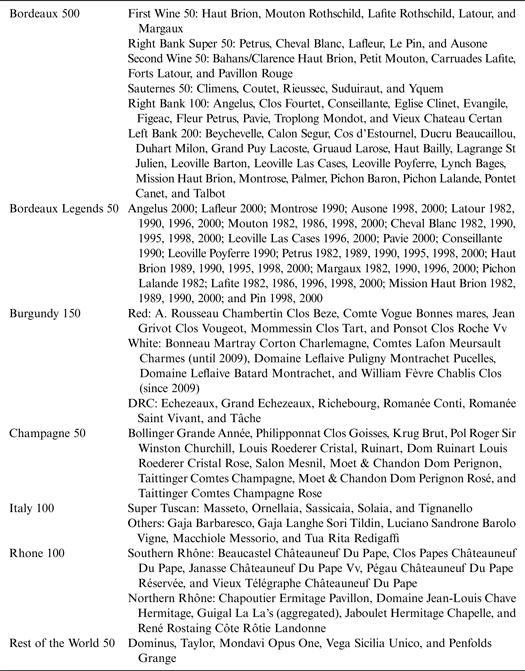
Wine indexes come from Liv-ex. We observed the Liv-ex Fine Wine 1000 and the seven subindexes it included over the period December 2003 to December 2013 (i.e., Bordeaux 500, Bordeaux Legends 50, Burgundy 150, Champagne 50, Italy 100, Rhone 100, and Rest of the World 50). We used the Liv-ex Fine Wine 1000 as a proxy for the global wine portfolio. In effect, the Liv-ex Fine Wine 1000 tracks 1,000 wines from across the world. It is calculated monthly and was rebased at 100 in December 2003. To qualify for the index, wines must have attracted a regular market on Liv-ex. They must also be physically available in the United Kingdom, so recent vintages that are only trading on an en primeur basis are ineligible. The wines included in the index are reviewed on a quarterly basis by committee. The Liv-ex Fine Wine 1000 is calculated using the Liv-ex Mid Price for each component wine. The Liv-ex Mid Price is calculated by finding the midpoint between the current highest bid price and lowest offer price on the Liv-ex trading platform. Each price is then verified by the valuation committee to ensure that the number is robust after taking into account all data, including merchant offer prices and historical Liv-ex transaction prices. The Liv-ex Fine Wine 1000 is price weighted at launch as follows: Bordeaux 500 (46%), Bordeaux Legends 50 (22%), Burgundy 150 (14%), Champagne 50 (3%), Italy 100 (7%), Rhone 100 (4%), and Rest of the World 50 (4%). Concerning these subindexes (see Table A1 in the Appendix for details about the components of each subindex), the Bordeaux 500 contains the 10 most recent physical vintages for the top 50 Bordeaux châteaux over the period 2001–2010,Footnote 5 the Bordeaux Legends 50 is a selection of 50 Bordeaux wines that are exceptional older vintages from before 1982, the Burgundy 150 includes the 10 most recent physical vintages of 15 white and red Burgundy wines, the Champagne 50 contains the most recent physical vintages of 12 Champagnes, the Italy 100 contains the 10 most recent physical vintages of the five “Super Tuscans” and five other leading Italian producers, the Rhone 100 is a selection of the 10 most recent physical vintages of five southern and five northern Rhône wines, and the Rest of the World 50 is a selection of the 10 most recent physical vintages of five wines from Spain, Portugal, the United States, and Australia. We converted the pound-denominated Liv-ex Fine Wine 1000 into a dollar-based series. To approximate the riskless asset, rf, we used the 3-month U.S. Treasury bills obtained from Bloomberg. This rate is annualized. We then divided it by 12 to obtain the monthly rate.
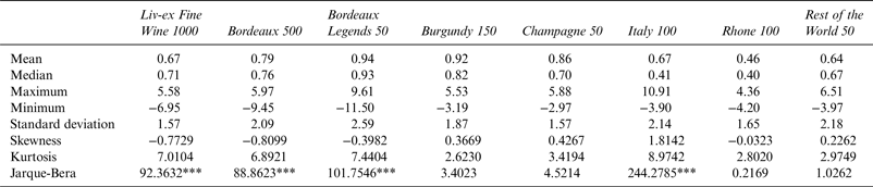
Table 1 details the main descriptive statistics for the Liv-ex indexes. The mean, median, maximum, minimum, and standard deviation are indicated in percentages. The mean returns of the eight indexes are all positive. The Champagne 50 and the Liv-ex Fine Wine 1000 have the lowest standard deviations, whereas the Bordeaux Legends 50 has the highest standard deviation. Skewness measures the asymmetry of the probability distribution; negative values for the Liv-ex Fine Wine 1000, Bordeaux 500, Bordeaux Legends 50, and Rhone 100 indicate that the data are skewed left. Kurtosis values greater than 3 mean that the distribution has fatter tails than a normal distribution, which is observed for the Liv-ex Fine Wine 1000, Bordeaux 500, Bordeaux Legends 50, and Italy 100. The null hypothesis for the Jarque-Bera test is that the distribution is normal. The test rejects the null hypothesis that the distribution is normal for Liv-ex Fine Wine 1000, Bordeaux 500, Bordeaux Legends 50, and Italy 100.
Descriptive Statistics for the Liv-ex Indexes (monthly returns)

Notes: Critical value for significance level of 5% = 5.5117. Asterisks indicate significance: *, P < 0.1; **, P < 0.05; ***, P < 0.01.
IV. Econometric Methodology
The risk premium is the expected return of a risky asset in excess of the return of a risk-free asset. Several techniques are used to calculate the risk premium. In this article, we use an extension of the standard CAPM of Sharpe (Reference Sharpe1964) and Lintner (Reference Lintner1965) to determine the risk premium for several wine indexes. The conditional CAPM, which takes conditional expectations into consideration, is as follows:
 $$E(R_{i,t}\left \vert {\Omega _t) - rf_t =\,} \right.\beta _i\;\left( {E\left( {R_{M,i}\left \vert {\Omega _t} \right.} \right) - rf_t} \right).$$
The empirical conditional CAPM equation is as follows:
 $$E(R_{i,t}\left \vert {\Omega _t) - rf_t =\,} \right.\beta _i\;\left( {E\left( {R_{M,t}\left \vert {\Omega _t} \right.} \right) - rf_t} \right) + \varepsilon _{i,t}.$$
In this model, Ω
t
is the information generated by the past values of ε
i,t
error terms; rf
t
is the one-period return of a riskless asset, approximated by the return of 3-month U.S. Treasury bills; and R
i,t
|Ω
t
and R
M,t
|Ω
t
are, respectively, the one-period returns of wine subindex i and the one-period wine market returns. In this framework, the Liv-ex Fine Wine 1000 is conditional to the common information set of the investor at the end of period t, where
 $\beta _{i,t} = {\mathop{\rm cov}} (R_{i,t},R_{m,t}\left\vert {\Omega _t} \right.){\mathop{\rm var}} (R_{m,t}\left\vert {\Omega _t} \right.)$
denotes the time-varying conditional market beta.
This article focuses on the application of the conditional CAPM to the wine market. The expected wine risk premium
 $E(R_{i,t}\left\vert {\Omega _t) - rf_t} \right.$
is measured relative to the return on the 3-month U.S. Treasury bill. The risk premium variability is due to the market's conditional variance,
 ${\mathop{\rm var}} (R_{m,t}\left\vert {\Omega _t} \right.)$
, and the conditional covariance between the wine subindex returns and the wine market returns (Liv-ex Fine Wine 1000Footnote
6
). We use the DCC-GARCH model to estimate the conditional variance and covariance.Footnote
7
We compared the GARCH model with several asymmetric GARCH models including EGARCH, GJR-GARCH, and threshold ARCH, taking several lag possibilities into account. According to the ARCH test, the Akaike information and Bayesian information criteria, and within the maximum likelihood criterion, GARCH (1,1) is the best model to estimate the model parameters. In this article, the estimation of the DCC-GARCH model is performed using a two-step procedure that allows for decreases in the complexity of the estimation process. In the first step, univariate GARCH models are estimated for each residual series of wine indexes. In the second step, residuals—transformed by their standard deviation estimated during the first stage—are used to estimate the parameters of the dynamic correlation. Engle, Shephard, and Shepard (Reference Engle, Shephard and Shepard2009) introduced a composite likelihood approach to covariance modeling, thus making the use of these methods plausible for large-scale applications. This approach resolves the bias problem of the two-step quasi-likelihood estimators. The composite likelihood is then maximized to determine the parameters of the DCC-GARCH. The advantage of this model is that it uses a dynamic multivariate distribution on top of the dynamic marginal distributions. This approach can be viewed as a simple type of dynamic copula approach without modeling distributions specifically.
For the DCC models, the number of parameters to be estimated is (N + 1) × (N + 4)/2, with N representing the number of variables that can be relatively higher if we choose a lag for the DCC model higher than 1. Thus, for simplicity and to overcome the difficulty of a large number of parameters, we estimated the DCC (1,1) GARCH (1,1).
Volatilities move together more or less closely over time across assets and markets. The extension from univariate GARCH models to multivariate GARCH has the advantage of providing more parsimonious estimators.
The time-varying risk premium for each wine index is determined using the DCC (1,1) GARCH (1,1) model. We use the composite likelihood approach developed by Engle, Shephard, and Shepard (Reference Engle, Shephard and Shepard2009) to estimate the DCC (1,1) GARCH (1,1) parameters. Following the methodology described in Engle and Shepard (Reference Engle and Sheppard2001), we obtained the residual returns using the regression model:
 $$r_{i,t} = a_0 + a_1r_{i,t - 1} + a_2r_{t - 1}^{Liv - ex1000} + \varepsilon _t.$$
In which r
i,t
is the return of each wine index and
 $r_{t - 1}^{Liv - ex1000} $
is the returns of the market index, the Liv-ex Fine Wine 1000. Then, using residual returns, ε
t
, the parameters of the DCC (1,1) GARCH (1,1) model are estimated.
The basic idea of the (DCC-)GARCH is that the covariance matrix H t in equation (4) can be split up into D t , a diagonal matrix of time-varying standard variation from univariate GARCH model, and a correlation matrix R t . In this model, both D t and R t are designed to be time varying. From the matrix H t , we determine the conditional volatility of each index, and from Q t in equation (6), the conditional variance covariance matrix of the standardized residuals. We estimate that the parameters a and b, respectively, determine the effects of shocks and dynamic correlations.
 $$H_t = D_tR_tD_t$$
 $$h_{i,t} = \omega _{i0} + \alpha _i\varepsilon _{i,t - q}^2 + \beta _ih_{i,t - j} $$
 $$Q_t\, = \left( {1 - a - b} \right)\overline {\,Q} + a\left( {\varepsilon _t\varepsilon _t^{\prime}} \right) + b{Q_{t - 1}}$$
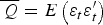
In equation (6),
 $\overline {\,Q} = E\left( {\varepsilon _t\varepsilon_t^{\prime}} \right)$
represents the unconditional variance covariance matrix that is time invariant.
V. Results and Comments
In order to check for time variation in wine return dynamics, we conducted an Engle's ARCH test (Table 2). This test allows for conditional heteroskedasticity of the residual series, using a lag of 1 in the alternative hypothesis. The null hypothesis states that no ARCH effects exist (i.e., there is homoskedasticity in the corresponding element of lags). The null hypothesis can be rejected at the 10% level for all the indexes.
Autoregressive Conditional Heteroskedasticity Test Lag 1

Notes: Critical value = 3.8415. Asterisks indicate significance: *, P < 0.1; **, P < 0.05; ***, P < 0.01. All h-test rejection decisions are not required.
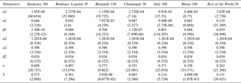
For the Liv-ex Fine Wine 1000 market index (Table 3), all of the estimated variables are statistically significant except for the constant terms. The a and b terms show the impact of past standardized shocks and lagged DCCs on the current DCCs. The necessary condition that a + b < 1 is verified for all the wine indexes. All the conditional correlations show significant variations over time except for the b parameter of the Burgundy 150 and Rhone 100. We can also note that the bivariate combinations are highly significant and significantly different from zero.
Estimation of DCC (1,1) GARCH (1,1) Model Parameters: Coefficient (T-statistic)

Note: DCC, dynamic conditional correlation; GARCH, generalized autoregressive conditional heteroskedasticity.
Figure 1 presents returns of wine indexes. In terms of the indexes' prices, practically all indexes follow the trend of the Liv-ex Fine Wine 1000. Figure 1 shows that the Bordeaux 500 is the index that is closest to the Liv-ex Fine Wine 1000. This is likely due to the importance of the Bordeaux 500 in the Liv-ex Fine Wine 1000. However, the Bordeaux Legends 50 index presents a different trend from the overall index. Indeed, its amplitude and volatility are higher than those of the overall index. The Burgundy 150 index and the Champagne 50 index also present higher amplitudes, whereas the Italy 100 index, the Rest of the World 50 index, and the Rhone 100 index all have lower amplitudes.
Wine Returns

Regarding returns, we see clearly that the Bordeaux 500 index and the Bordeaux Legends 50 index present the same trend as the Liv-ex Fine Wine 1000. This is likely due to the importance of Bordeaux wines in the overall index, as mentioned previously. However, we note that the Bordeaux Legends 50 index presents a significantly higher returns maximum (at the end of the year 2006). Other indexes present no similar trend relative to the overall index. The volatility in these indexes is very important. If we exclude the decrease in returns from 2008, then all annual returns fall between −3% and +6%. The Italy 100 index presents very significant returns until 2005, during which its monthly returns were as high as 11%. The decrease in returns from the second quarter of 2008 through the end of the year is visible for all indexes. Surprisingly, this decrease is less significant in the subindexes than it is in the overall index, except for the subindexes of Bordeaux. Thus, it seems that the Bordeaux fine wines are less volatile in “normal” periods but riskier during a crisis.
As mentioned previously, we use the bivariate DCC-GARCH model to determine the variable risk premium and to discuss the impact on returns of the wine market. We know that a GARCH structure is used for modeling the correlation dynamics with a β parameter.
As explained in the previous section, systematic risk beta is mainly explained by the volatility of the market portfolio. We estimate the time-varying beta from the matrix H t as
 $$\beta _{i,t} = \displaystyle{{{\hat H}_{12,t}} \over {{\hat H}_{22,t}}}$$
with
 $\hat H_{22,t}$
and
 $\hat H_{12,t}$
, respectively, representing the conditional volatilities of the global portfolio market and the conditional covariance between the wine subindex i and the global portfolio market m. The time-varying equity risk premium for each index is determined by multiplying β
ti
by the market risk premium
 $(R_{tm} - R_{tf})$
.
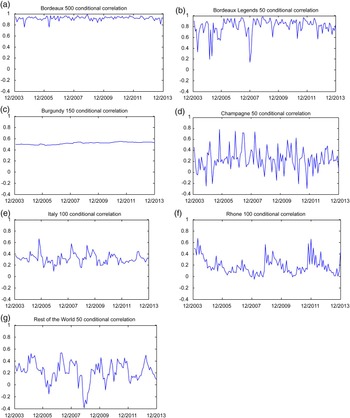
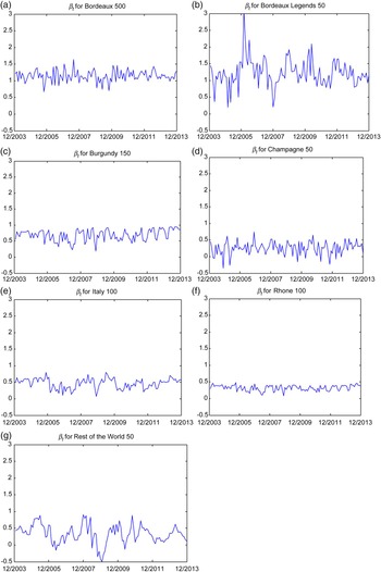
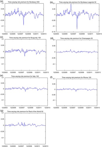
Figure 2 presents the DCCs. Although Bordeaux 500 and Bordeaux Legends 50 present the highest conditional correlation, Rhone 100 and Italy 100 show the lowest level of conditional correlation, with some peaks at 0.7. Only the Rest of the World 50 index presents negative conditional correlation with the Liv-ex Fine Wine 1000 that represents the global wine market. Figure 3 shows the time-varying beta for all wine indexes, and Figure 4 shows that the risk premium estimated is volatile. Indeed, the Bordeaux 500 index, the Bordeaux Legends 50 index, and the Burgundy 150 index present the highest mean of time-varying betas (Table 4). The greater systematic risks for both of the Bordeaux wine indexes confirm the fact that most wine investments focus on Bordeaux wines. These results do not confirm the betas found by Masset and Weisskopf (Reference Masset and Weisskopf2010) and Sanning, Shaffer, and Sharratt (Reference Sanning, Shaffer and Sharratt2008), which oscillated around zero. Masset and Weisskopf (Reference Masset and Weisskopf2010) found that betas drop below zero in a crisis period. They estimated that the addition of fine wine in portfolios reduces exposure to systematic risk. Their results come from comparisons with the Russell 3000 financial index, whereas we used the Liv-ex Fine Wine 1000 as a benchmark. Thus, we investigated the properties of each subindex in comparison with the wine market, not the equity market. Figure 3 indicates that these subindexes present the highest level of risk premium. These indexes are the riskiest and therefore induce market volatility. The increase in time-varying beta is seen among investors as an additional risk to bear in holding wine in the indexes. Therefore, the increase in their equity premiums, as shown in Figure 3, reflects that rational investor demand presents higher returns to hedge against the risk of a financial crisis.
Dynamic Conditional Correlations

Time-Varying Betas

Time-Varying Risk Premium

Mean Beta and Mean Risk Premium

The values of the conditional betas of the Champagne 50, Italy 100, Rhone 100, and Rest of the World 50 indexes are weak in comparison with those of the Bordeaux and Burgundy indexes. Agreeing with Fogarty (Reference Fogarty2010) and Kourtis, Markellos, and Psychoyios (Reference Kourtis, Markellos and Psychoyios2012), our results confirm that these wines are not the most traded and asked for on the market. Therefore, their systematic risks and risk premiums are not very high.
The conditional beta of the Rest of the World 50 index becomes negative during market downturns. This index is composed of Australian (Penfolds Grange), American (Dominus, Mondavi Opus One, and Taylor), and Sicilian (Vega Sicilia) wines. This index and the Champagne 50 index (in 2004 and 2005) are the lone indexes to present negative betas. The negative beta indicates that this index has evolved in the inverse direction of the market index. When the Liv-ex Fine Wine 1000 declined during this period, the Rest of the World 50 index rose. This same observation can be made regarding the risk premiums in Figure 4.
We are particularly interested in the financial crisis that began in September 2008 and spread to the Eurozone. Indeed, with the exception of a small percent represented by Australian and American wines, the Liv-ex Fine Wine 1000 is composed primarily of European wines in the Eurozone (France, Italy, and Portugal). Not all wines behaved in the same way at the beginning of the financial crisis of 2008–2009. Indeed, the betas of the Bordeaux wines and the Rest of the World 50 index decreased to between 0 and 0.2 following the fall of the financial market. However, these betas returned to more normal values immediately after this downturn. The beta of the Rest of the World 50 index became negative at the beginning of the financial crisis. At the time at which the financial crisis was announced, the betas of Bordeaux wines had an inverse trend in comparison with the other wines; the beta for the Bordeaux 500 index notably increased following the formal announcements of three significant wine market declines in 2009. Finally, Figure 4 permits us to characterize the market decline. Indeed, time-varying risk premiums became strongly negative at the end of the third quarter of 2008, whatever the appellation. We also note negative time-varying risk premiums to be less important during the third quarter of 2011 and during the spring of 2012.
VI. Conclusions
The rapid global expansion of fine-wine investments, the 2008 financial crisis, and the search for alternative investments have increased the need to understand the price risk and risk premium of the fine-wine market. This article has examined the time-varying risk premium in the context of investments in fine wines. We focused our analysis on the behavior of the main wine indexes used by investors, merchants, funds, and speculators. Using a conditional CAPM and a DCC-GARCH model (which appears to provide a strong framework for analyzing DCCs), we calculated time-varying betas and time-varying risk premiums for several appellations of wine. Our study is the first to use this methodology by applying it to the fine-wine market. This model allows us to analyze the conditional correlation for the main wine indexes with the market. Therefore, this research is innovative in this context. We found different betas in comparison with the main previous studies on this topic. Several main practical implications for investors can be advanced for Bordeaux wines. First, Bordeaux wines were observed to amplify the investment effects of the financial crisis, most notably wines represented by the Bordeaux Legends 50 index. Second, Bordeaux wines are less volatile in no-crisis periods. Third, the greater systematic risk exhibited by Bordeaux wines confirmed that most wine investments focus on this submarket. Fourth, after Bordeaux wines, Burgundy wines are the most traded and most volatile. Finally, in a crisis period wines from the rest of the world present the possibility to invest in alternative assets that show an inverse trend to the fine-wine market. Future research could investigate specific châteaux and alternative types of derivatives such as options, futures, or swaps as ways to hedge investors against market volatility.
Appendix
Components of Each Subindex of the Liv-ex Fine Wine 1000

Source: Liv-ex. Available at: https://www.liv-ex.com/staticPageContent.do?pageKey=Fine_Wine_1000
The Dynamic Conditional Correlation Generalized Autoregressive Conditional Heteroskedasticity Model
The dynamic conditional correlation (DCC) generalized autoregressive conditional heteroskedasticity (GARCH) model is as follows:
 $$r_t = \mu _t + a_t,$$
where r
t
is the return vector, μ
t
is the vector of expected value of the conditional r
t
, and a
t
is the vector of mean-corrected returns of n assets at time t,
 $E\left( {a_t} \right) = 0$
, and
 ${\mathop{\rm cov}} \left( {a_t} \right) = H_t$
:
 $$a_t = H_t^{1/2} z_t,$$
where H
t
is a matrix of conditional variances of a
t
at time t, and z
t
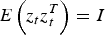
vector of iid errors such that
 $E\left( {z_t} \right) = 0$
and
 $E\left( {z_tz_t^T} \right) = I$
, the identity matrix.
 $$H_t = D_t R_tD_t,$$
where D t is a diagonal matrix of time-varying standard deviation from the univariate GARCH model.
 $$D_t = \left[ {\matrix{ {\sigma _{1t}} & 0 & 0 & \ldots & 0 \cr 0 & {\sigma _{2t}} & {} & \cdots & 0 \cr 0 & 0 & {\sigma _{3t}} & {} & \vdots \cr \vdots & \vdots & {} & \ddots & 0 \cr 0 & 0 & \cdots & 0 & {\sigma _{nt}} \cr}} \right],$$
where h
i,t
evolves according to the univariate GARCH of the form
 $h_{i,t} = \omega _{i0} + \sum\limits_{j = 1}^{p_i} {\alpha _{iq}\varepsilon _{i,t - q}^2} + \sum\limits_{j = 1}^{q_i} {\beta _{ip}h_{i,t - j}} $
. The term h
i,t
is not limited to the standard univariate GARCH (p,q) and can include any GARCH process with Gaussian distributed errors that satisfy appropriate stationarity conditions that ensure that the unconditional variance exists.
R
t
is the matrix of conditional correlation of the standardized residuals
 $\varepsilon _t = D_t^{ - 1} r_t \to N\left( {0,R_t} \right)$
:
 $$R_t = \left[ {\matrix{ 1 & {\varphi _{12,t}} & {\varphi _{13,t}} & \ldots & {\varphi _{1n,t}} \cr {\varphi _{21,t}} & 1 & {\varphi _{23,t}} & \cdots & {\varphi _{2n,t}} \cr {\varphi _{31,t}} & {\varphi _{32,t}} & 1 & {} & {\varphi _{3n,t} \vdots} \cr \vdots & \vdots & {} & \ddots & \vdots \cr {\varphi _{n1,t}} & {\varphi _{n2,t}} & {\varphi _{n3,t}} & \cdots & 1 \cr}} \right].$$
A GARCH structure is used for modeling the correlation dynamics. The DCC process of order (M,N) can be described in the following equations:
 $$R_t = \left( {Q_t^{\ast}} \right)^{ - 1}Q_t\,\left( {Q_t^{\ast}} \right)^{ - 1},$$
 $$Q_t\, = \left( {1 - \sum\limits_{m = 1}^M {a_m - \sum\limits_{n = 1}^N {b_n}}} \right)\overline {\,Q} + \sum\limits_{m = 1}^M {a_m\left( {\varepsilon _{t - m}\varepsilon _{t - m}^{\prime}} \right)} + \sum\limits_{n = 1}^N {b_nQ_{1 - n}}, $$
where
 $\overline Q = E\left( {\varepsilon _t\varepsilon _t^{\prime}} \right)$
represents the unconditional variance covariance matrix, which is time invariant. The parameters a and b, respectively, determine the effects of shocks and dynamic correlations.
 $Q_t^{\ast} $
is a diagonal matrix containing the square root of the diagonal elements of
 $Q_t$
.
 $$Q_t^{^\ast} = \left[ {\matrix{ {\sqrt {q_{11,t}}} & 0 & 0 & \ldots & 0 \cr 0 & {\sqrt {q_{22,t}}} & 0 & \cdots & 0 \cr 0 & 0 & {\sqrt {q_{33,t}}} & 0 & {0 \vdots} \cr \vdots & \vdots & 0 & \ddots & \vdots \cr 0 & 0 & 0 & \cdots & {\sqrt {q_{nn,t}}} \cr}} \right]$$