1. Introduction
The characterization of intrinsic properties and rheological responses of highly viscous films on the surface of liquids, such as biofilms (micro-organisms at the air–water interface), lung surfactants (mixtures of lipids and proteins), and polymeric films that are essential in numerous applications, continues to garner significant attention (Krägel, Derkatch & Miller Reference Krägel, Derkatch and Miller2008; Krägel & Derkatch Reference Krägel and Derkatch2010; Langevin Reference Langevin2014a ,Reference Langevin b ). The most sensitive method for measuring surface (excess) shear viscosity is the deep-channel surface viscometer (Mannheimer & Schechter Reference Mannheimer and Schechter1970; Edwards, Brenner & Wasan Reference Edwards, Brenner and Wasan1991), where the film at the air–water interface is sheared by the viscous coupling to the bulk flow that is driven by the rotating floor (Lopez & Hirsa Reference Lopez and Hirsa1998). However, the deep-channel flow fails to shear highly viscous films, as the vortex lines become parallel to the interface and the film becomes immobile. Some other approaches involve directly shearing the film using a knife edge or a magnetic needle in contact with the surface film, but interpreting the results is non-trivial due to the coupling with the bulk flow (Reynaert et al. Reference Reynaert, Brooks, Moldenaers, Vermant and Fuller2008).
In interfacial rheology, often the goal is to find a shearing interfacial flow that is as decoupled as possible from the bulk flow. However, there is intrinsic interest in such driven bulk flows since there are many situations where one desires bulk flows in the absence of moving solid walls. Solid boundaries influence liquids in a myriad of ways through chemical, sorption and electrostatic interactions. For example, solid walls influence protein folding and can denature protein. There are different design strategies for bioreactors to address these issues (Hambor Reference Hambor2012). The bioreactor type largely depends on whether the cells are growing as single cells in suspension, in monolayers, or in cell aggregates. A system essentially free of boundaries would provide many advantages over conventional systems, including gas exchange and nutrient transport.
There are only a few studies that discuss or take into account the coupling to the bulk flow that is driven by a knife edge or a needle (Reynaert et al. Reference Reynaert, Brooks, Moldenaers, Vermant and Fuller2008; Vandebril et al. Reference Vandebril, Franck, Fuller, Moldnaers and Vermant2010; Verwijlen et al. Reference Verwijlen, Moldenaers, Stone and Vermant2011; Lopez & Hirsa Reference Lopez and Hirsa2015), and we are not aware of any detailed measurements of such bulk flows. Here, we utilize the knife edge for several reasons. In the experiment, the knife edge can be carefully treated so that there is no meniscus and the interface can be made essentially flat down to the mesoscale (order of a micron, which is essentially the limit of optical microscopy). Also, we have a numerical code based on a Newtonian surface model that is nonlinearly coupled to the bulk flow and includes the effects of inertia via the Navier–Stokes equations (Lopez & Hirsa Reference Lopez and Hirsa2015). The model predictions are compared to measurements in the bulk flow using particle image velocimetry. For the present study, we use DPPC (dipalmitoylphosphatidylcholine) to form monomolecular films on the surface of water. DPPC is an amphiphilic molecule with twin hydrophobic tails which can form highly insoluble films on the surface of water. There is a vast body of literature on DPPC films (von Tscharner & McConnell Reference von Tscharner and McConnell1981; Helm et al. Reference Helm, Kjaer, Mohwald and Als-Nielsen1987; Dluhy et al. Reference Dluhy, Reilly, Hunt, Mitchell, Mautone and Mendelsohn1989; McConnell Reference McConnell1991; Sundaram et al. Reference Sundaram, Ferri, Vollhardt and Stebe1998; Dynarowicz-Latka, Dhanabalan & Oliveira Reference Dynarowicz-Latka, Dhanabalan and Oliveira2001; Wüstneck et al. Reference Wüstneck, Wüstneck, Pison, Fainerman and Miller2001; Ding, Warriner & Zasadzinski Reference Ding, Warriner and Zasadzinski2002a ; Ding et al. Reference Ding, Warriner, Zasadzinski and Schwartz2002b ; Roke et al. Reference Roke, Schins, Müller and Bonn2003; Aroti et al. Reference Aroti, Leontidis, Maltseva and Brezesinski2004; Baoukina et al. Reference Baoukina, Monticelli, Risselada, Marrink and Tieleman2008; Nishimura et al. Reference Nishimura, Magana, Ketelson and Fuller2008; Walder, Levine & Dennin Reference Walder, Levine and Dennin2008; Choi et al. Reference Choi, Steltenkamp, Zasadzinski and Squires2011; Hermans & Vermant Reference Hermans and Vermant2014), the motivation being in part because it is the most prevalent component of lung surfactant. Furthermore, DPPC is widely studied because it is ubiquitous in bilayers that form cell walls. Transport across and within cell walls is of fundamental interest to biology and medicine, and the viscosity of DPPC plays a central role.
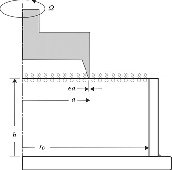
Schematic of the flow apparatus.

2. Flow configuration, theory, experiments and numerics
2.1. Governing equations
Figure 1 shows a schematic of the flow system, consisting of a stationary cylinder of radius
 $r_{o}$
filled to a height
 $h$
with water of kinetic viscosity
 ${\it\nu}$
and dynamic viscosity
 ${\it\mu}$
. The air–water interface is covered by a thin film. A sharp circular knife edge, of radius
 $a$
and thickness
 ${\it\epsilon}a$
is in contact with the interfacial film, but does not penetrate into the bulk, and is rotating at constant angular speed
 ${\it\Omega}$
.
The flow in the bulk is governed by the Navier–Stokes equations. For the parameter regimes considered experimentally in this study, the flow remains axisymmetric, and it is convenient to write the equations using a streamfunction–vorticity formulation in cylindrical coordinates
 $\boldsymbol{r}=(r,{\it\theta},z)$
, where the velocity in terms of the streamfunction,
 ${\it\psi}$
, and angular momentum,
 ${\it\gamma}$
, is
 $$\begin{eqnarray}\boldsymbol{u}=(u,v,w)=\left(-\frac{1}{r}\frac{\partial {\it\psi}}{\partial z},\frac{{\it\gamma}}{r},\frac{1}{r}\frac{\partial {\it\psi}}{\partial r}\right),\end{eqnarray}$$
and the vorticity is
 $$\begin{eqnarray}\boldsymbol{{\rm\nabla}}\times \boldsymbol{u}=\left(-\frac{1}{r}\frac{\partial {\it\gamma}}{\partial z},{\it\eta},\frac{1}{r}\frac{\partial {\it\gamma}}{\partial r}\right),\end{eqnarray}$$
where the azimuthal vorticity is
 $$\begin{eqnarray}{\it\eta}=-\frac{1}{r}\left(\frac{\partial ^{2}{\it\psi}}{\partial z^{2}}+\frac{\partial ^{2}{\it\psi}}{\partial r^{2}}-\frac{1}{r}\frac{\partial {\it\psi}}{\partial r}\right).\end{eqnarray}$$
Using the radius of the knife edge,
 $a$
, as the length scale and
 $1/{\it\Omega}$
as the time scale, the non-dimensional Navier–Stokes equations in streamfunction–vorticity form are
 $$\begin{eqnarray}\displaystyle & \displaystyle \frac{\partial {\it\gamma}}{\partial t}-\frac{1}{r}\frac{\partial {\it\psi}}{\partial z}\frac{\partial {\it\gamma}}{\partial r}+\frac{1}{r}\frac{\partial {\it\psi}}{\partial r}\frac{\partial {\it\gamma}}{\partial z}=\frac{1}{Re}\left(\frac{\partial ^{2}{\it\gamma}}{\partial z^{2}}+\frac{\partial ^{2}{\it\gamma}}{\partial r^{2}}-\frac{1}{r}\frac{\partial {\it\gamma}}{\partial r}\right)\!, & \displaystyle\end{eqnarray}$$
 $$\begin{eqnarray}\displaystyle & \displaystyle \frac{\partial {\it\eta}}{\partial t}-\frac{1}{r}\frac{\partial {\it\psi}}{\partial z}\frac{\partial {\it\eta}}{\partial r}+\frac{1}{r}\frac{\partial {\it\psi}}{\partial r}\frac{\partial {\it\eta}}{\partial z}+\frac{{\it\eta}}{r^{2}}\frac{\partial {\it\psi}}{\partial z}-\frac{2{\it\gamma}}{r^{3}}\frac{\partial {\it\gamma}}{\partial z}=\frac{1}{Re}\left(\frac{\partial ^{2}{\it\eta}}{\partial z^{2}}+\frac{\partial ^{2}{\it\eta}}{\partial r^{2}}+\frac{1}{r}\frac{\partial {\it\eta}}{\partial r}-\frac{{\it\eta}}{r^{2}}\right)\!,\qquad & \displaystyle\end{eqnarray}$$
 $Re={\it\Omega}a^{2}/{\it\nu}$
is the Reynolds number, giving the ratio of the viscous time in the bulk to the knife-edge rotation time.
Geometric parameters governing this flow are the cylinder-to-knife-edge radius ratio
 $R=r_{o}/a$
, the cylinder-height-to-knife-edge radius ratio
 $H=h/a$
, and the knife-edge-thickness-to-radius ratio
 ${\it\epsilon}$
. How the flow depends on these has been described in the numerical study in Lopez & Hirsa (Reference Lopez and Hirsa2015), and in this paper, we shall use values of these that correspond to the specific experiments that are reported below.
The boundary conditions in the bulk are no-slip:
 $$\begin{eqnarray}\displaystyle & \displaystyle \text{Sidewall},r=R:\quad {\it\gamma}={\it\psi}=0,{\it\eta}=-\frac{1}{R}\frac{\partial ^{2}{\it\psi}}{\partial r^{2}}, & \displaystyle\end{eqnarray}$$
 $$\begin{eqnarray}\displaystyle & \displaystyle \text{Bottom},z=0:\quad {\it\gamma}={\it\psi}=0,{\it\eta}=-\frac{1}{r}\frac{\partial ^{2}{\it\psi}}{\partial z^{2}}, & \displaystyle\end{eqnarray}$$
 $$\begin{eqnarray}\displaystyle & \displaystyle \text{Axis},r=0:\quad {\it\gamma}={\it\psi}=0,\frac{\partial {\it\eta}}{\partial r}=0, & \displaystyle\end{eqnarray}$$
The air–water interface is assumed to remain flat; this is a very good approximation for the range of flow parameters considered experimentally. The interface is modelled using the Boussinesq–Scriven surface model (Scriven Reference Scriven1960; Edwards et al. Reference Edwards, Brenner and Wasan1991; Slattery, Sagis & Oh Reference Slattery, Sagis and Oh2007), in which the surface stress tensor is
 $$\begin{eqnarray}\unicode[STIX]{x1D64F}^{s}=({\it\sigma}+({\it\kappa}^{s}-{\it\mu}^{s})\boldsymbol{{\rm\nabla}}_{s}\boldsymbol{\cdot }\boldsymbol{u}^{s})\unicode[STIX]{x1D644}_{s}+{\it\mu}^{s}(\boldsymbol{{\rm\nabla}}_{s}\boldsymbol{u}^{s}\boldsymbol{\cdot }\unicode[STIX]{x1D644}_{s}+\unicode[STIX]{x1D644}_{s}\boldsymbol{\cdot }(\boldsymbol{{\rm\nabla}}_{s}\boldsymbol{u}^{s})^{\text{T}}),\end{eqnarray}$$
where
 ${\it\sigma}$
is the equilibrium surface tension,
 ${\it\mu}^{s}$
is the surface shear viscosity,
 ${\it\kappa}^{s}$
is the surface dilatational viscosity,
 $\boldsymbol{u}^{s}$
is the surface velocity vector,
 $\boldsymbol{{\rm\nabla}}_{s}$
is the surface gradient operator, and
 $\unicode[STIX]{x1D644}_{s}$
projects any vector onto the interface. For a flat interface, only the tangential stress balance plays a dynamic role. The non-dimensional tangential stress balance, at the interface
 $z=H$
, in the azimuthal direction is
 $$\begin{eqnarray}\frac{\partial v}{\partial z}=\hat{{\it\mu}}^{s}\left(\frac{\partial ^{2}v}{\partial r^{2}}+\frac{1}{r}\frac{\partial v}{\partial r}-\frac{v}{r^{2}}\right)+\frac{\partial \hat{{\it\mu}}^{s}}{\partial r}\left(\frac{\partial v}{\partial r}-\frac{v}{r}\right),\end{eqnarray}$$
and in the radial direction is
 $$\begin{eqnarray}{\it\eta}=\frac{1}{Ca}\frac{\partial \hat{{\it\sigma}}}{\partial r}+(\hat{{\it\mu}}^{s}+\hat{{\it\kappa}}^{s})\left(\frac{1}{r^{2}}\frac{\partial ^{2}{\it\psi}}{\partial r\partial z}-\frac{1}{r}\frac{\partial ^{3}{\it\psi}}{\partial r^{2}\partial z}\right)-\frac{1}{r}\frac{\partial ^{2}{\it\psi}}{\partial r\partial z}\frac{\partial (\hat{{\it\mu}}^{s}+\hat{{\it\kappa}}^{s})}{\partial r}+\frac{2}{r^{2}}\frac{\partial {\it\psi}}{\partial z}\frac{\partial \hat{{\it\mu}}^{s}}{\partial r},\end{eqnarray}$$
where
 $Ca={\it\mu}{\it\Omega}a/{\it\sigma}_{0}$
is the capillary number,
 $\hat{{\it\sigma}}={\it\sigma}/{\it\sigma}_{0}$
,
 ${\it\sigma}_{0}$
is the surface tension of the interface in the absence of a film,
 $\hat{{\it\mu}}^{s}={\it\mu}^{s}/{\it\mu}a$
and
 $\hat{{\it\kappa}}^{s}={\it\kappa}^{s}/{\it\mu}a$
. We have previously demonstrated through experiments and computations (Lopez & Hirsa Reference Lopez and Hirsa2000; Hirsa, Lopez & Miraghaie Reference Hirsa, Lopez and Miraghaie2001, Reference Hirsa, Lopez and Miraghaie2002) that, at steady state, only a minuscule amount of Marangoni stress is required in order for the surface tension gradient to eliminate any radial component of surface velocity. This is due to the small capillary number in the flows of interest (Hirsa et al.
Reference Hirsa, Lopez and Miraghaie2002). This was shown in a deep-channel viscometer geometry consisting of an annular region bounded by stationary cylinders and a rotating floor. The secondary meridional flow is much weaker in the present knife-edge geometry than in the deep-channel geometry, and at steady state the radial component of velocity is essentially zero at the interface. Under such conditions, (2.11) is replaced by
 $$\begin{eqnarray}{\it\eta}=-\frac{1}{r}\frac{\partial ^{2}{\it\psi}}{\partial z^{2}},\end{eqnarray}$$
any concentration gradients of the surface film are negligible, and the surface dilatational viscosity no longer appears in the governing equations. Then,
 $\hat{{\it\mu}}^{s}$
is often termed the Boussinesq number
 $Bo={\it\mu}^{s}/{\it\mu}a$
, and the azimuthal tangential stress equation at the interface reduces to
 $$\begin{eqnarray}\frac{\partial v}{\partial z}=Bo\left(\frac{\partial ^{2}v}{\partial r^{2}}+\frac{1}{r}\frac{\partial v}{\partial r}-\frac{v}{r^{2}}\right).\end{eqnarray}$$
The question of what length scale to use to define
 $Bo$
is often considered in the literature (e.g. Fitzgibbon et al.
Reference Fitzgibbon, Shaqfeh, Fuller and Walker2014). The Boussinesq number
 $Bo$
gives a ratio of surface viscosity to bulk viscosity, and to make it non-dimensional requires a length scale. For consistency, the same length scale used to non-dimensionalize all quantities in the model equations should be used, resulting in dimensionless numbers
 $Bo$
and
 $Re$
, as well as the geometric ratios (knife-edge thickness to knife-edge radius ratio, knife-edge radius to cylinder radius ratio, and cylinder depth-to-radius ratio). Using a different length scale to non-dimensionalize the viscosity ratio, for example the knife-edge thickness instead of its radius, would result in a new Boussinesq number,
 $Bo^{\ast }={\it\mu}^{s}/({\it\mu}{\it\epsilon}a)=Bo/{\it\epsilon}$
, and the
 $Bo$
in (2.13) is replaced with
 ${\it\epsilon}Bo^{\ast }$
. Using the knife-edge thickness instead of its radius to define the Boussinesq number becomes problematic in the limit of the thickness going to zero. Retaining the
 $Bo$
using the radius as the length scale, one can examine effects of variations in
 $Bo$
with a zero thickness knife edge, as was done numerically in Lopez & Hirsa (Reference Lopez and Hirsa2015).
2.2. Experimental apparatus and methods
The experiments were performed in a glass dish assembly. The floor of the dish consisted of a 75 mm diameter, 3 mm thick optical window with a ‘quarter wave’ surface accuracy (
 $0.1~{\rm\mu}\text{m}$
). A precision glass cylinder (Ace Glass, Trubore 8700-84) with an inside diameter
 $2r_{o}=50.06\pm 0.01~\text{mm}$
was cut to a height
 $h=25.40\pm 0.03~\text{mm}$
. To achieve this accuracy and ensure that its ends are orthogonal to the axis, the ends were ground as the cylinder was held by a jig in a vertical mill and manually rotated slowly as it was gradually lowered onto a high-speed die grinder with a silicon oxide wheel. The precision ground ends of the glass cylinder were subsequently polished smooth with wet ‘600 grit’ and then ‘1000 grit’ sandpaper. Finally, the glass cylinder was sealed on the outside to ensure that it made intimate contact with the optical-window floor and therefore at a right angle.
The knife edge was cutoff from a stainless steel (type 440c) precision bushing stock (McMaster-Carr, 1991T21) and the end was machined to an accuracy of
 $\pm 0.03~\text{mm}$
. The knife edge had a diameter
 $2a=25.40\pm 0.01~\text{mm}$
and thickness
 ${\it\epsilon}a=0.25\pm 0.02~\text{mm}$
, resulting in a thickness ratio of
 ${\it\epsilon}=0.02$
. The knife edge was attached to a precision ground shaft supported by a pair of high precision (ABEC-7) ball bearings, which were positioned 10 cm apart in a precision machined block of aluminium. The shaft was spun by a fine-tooth timing belt and pulley assembly driven by a stepper motor. To ensure smooth motion, the stepper motor was micro-stepped and utilized a flywheel. A dilute solution of paraffin in hexane was applied to the sides of the knife edge in order to make it highly hydrophobic. After the evaporation of hexane, a very thin (invisible) coating of paraffin covered the sides of the knife edge. The bottom of the knife edge was cleaned with high-purity hexane to ensure intimate contact with the water surface. The knife-edge assembly was mounted on a linear micro-stage so that it could be detached from the surface of water prior to the spreading of the monolayer film. The water level was set and checked with a sharp needle mounted on a linear micro-stage to an accuracy of 0.025 mm. Finally, the position of the knife edge relative to the water surface was set while viewing the flow apparatus from the side using a horizontally mounted, long-standoff-distance microscope (Wild Makroskope, M420 with APO Zoom lens) at a total magnification of approximately
 $100\times$
.
Particle image velocimetry (PIV) was utilized to measure the flow field. Illumination was from a frequency-doubled (532 nm) Nd:YAG laser (New Wave, Solo I-15 PIV). The beam was thinned with a 101.6 mm focal length bi-convex lens and spread into a sheet with a
 $-50.8~\text{mm}$
focal length plano-cylindrical lens. The maximum thickness (in the
 $z$
axial direction) of the light sheet in the field of view was 0.3 mm, or approximately
 $0.025a$
; this is comparable to the thickness of the knife edge. The lens train was mounted on an optical platform adjusted by a micrometer so that the depth at which the (horizontal) light sheet entered the cylinder could be adjusted to an accuracy of 0.03 mm. The light sheet was imaged from beneath, through the optical floor. A right-angle prism was utilized so that the camera and its lens assembly could be mounted horizontally on the optical table on which the experiments were conducted. A black-and-white, high-speed camera was utilized (Redlake, HG-100K) along with a Micro-Nikkor 105 mm,
 $f/4$
lens. The time delay utilized for the experiments at
 $Re=30$
, 100 and 300 were 200, 66.7 and 23.9 ms, respectively. The spatial resolution for all the images was
 $35~{\rm\mu}\text{m}~\text{pixel}^{-1}$
. The images were analysed using the open-source software PIVLab, utilzing a multi-pass algorithm starting with an interrogation window size of
 $64\times 64$
pixels and finishing with
 $16\times 16$
pixels. Each pass used a 50 % window overlap.
De-ionized (DI) water of resistivity greater than
 $18~\text{M}{\rm\Omega}~\text{cm}$
and total organic carbon less than 5 ppb (Millipore, Simplicity 185-UV, fed with Poland Spring distilled water) was used for all the experiments. The experiments were all conducted at
 $22\pm 1\,^{\circ }\text{C}$
, where the kinematic viscosity of water is
 ${\it\nu}=0.00957~\text{cm}^{2}~\text{s}^{-1}$
. The water was seeded with
 $4~{\rm\mu}\text{m}$
fluorescent latex beads (Thermo-Fisher Life Technologies, F-8859) which have peak excitation in green, matching the laser wavelength, and peak emissions in yellow. These particles are sulphate stabilized and can be cleaned of all surfactants without any noticeable aggregation. The particles were cleaned as follows: the suspension in the original container was first placed in a sonication bath for 30 s;
 $150~{\rm\mu}\text{l}$
was withdrawn and added to 10 ml of DI water in a test tube and centrifuged (1550 RPM) for at least 300 s. The particles, which have a specific gravity greater than unity, accumulate at the bottom of the test tube. The supernatant water was aspirated, leaving cleaner particles at the bottom. Fresh DI water was added and the suspension was centrifuged, followed by aspiration. This process was repeated two more times. Subsequently, the particles were cleaned by centrifugation and aspiration using reagent grade acetone, and then HPLC-grade methanol. After the supernatant methanol was aspirated, the particles were allowed to fully dry to guard against methanol contamination of water in the experiments. The dried seeding particles were subsequently resuspended in 10 ml of DI water, sonicated to breakup any aggregates, and finally added to 1 l of DI water, giving a final concentration of less than 4 ppm.
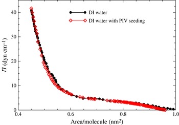
Equation of state of DPPC monolayer on water, with and without seeding for PIV, measured in a Langmuir trough during a slow compression.

The equation of state for DPPC on water, in terms of surface pressure
 ${\it\Pi}$
(surface tension of the clean interface minus the surface tension of the film-covered interface) and area coverage per molecule, is presented in figure 2. The details of how DPPC films were formed are presented in the Appendix. The surface tension was measured using a Wilhelmy plate during slow compression in a Langmuir trough (Vogel & Hirsa Reference Vogel and Hirsa2002). The equations of state measured on pure water (DI) and water with PIV seeding particles were compared to illustrate that the seeding particles have no dynamic effect on the interfacial film. The equation of state is not needed for the modelling in the range of surface pressures considered in this study.
2.3. Numerical methods
The numerical technique used is the same as that implemented in Lopez & Hirsa (Reference Lopez and Hirsa2015), and only a brief overview is presented here. The Navier–Stokes equations, (2.4) and (2.5), for the bulk flow are solved using a second-order finite difference scheme for space together with a second-order predictor–corrector scheme for time evolution. The interfacial flow is solved using one-sided differences from the bulk flow to compute
 $\partial v/\partial z$
at the interface for the left-hand side of (2.13). The experiments were conducted in a cylinder of depth-to-radius ratio of one, and we used
 $n_{r}=n_{z}=200$
grid points in each of the radial and axial directions. The radius of the knife edge was half of the radius of the cylinder, and its thickness was 2 % of the knife radius, so the knife edge was two grid points thick. The time step used was
 ${\it\delta}t=2\times 10^{-3}$
for
 $Re=100$
and
 $Re=300$
, and
 ${\it\delta}t=2\times 10^{-4}$
for
 $Re=30$
. Grid resolution tests were conducted in Lopez & Hirsa (Reference Lopez and Hirsa2015), where it was concluded that
 $n_{r}=n_{z}=100$
was adequate for these flows in these
 $Re$
and
 $Bo$
ranges; here we used double that resolution.
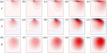
Computed contours of
 ${\it\gamma}$
(vortex lines; (a–e)),
 ${\it\eta}$
(azimuthal vorticity; (f–j)), and
 ${\it\psi}$
(streamlines; (k–o)), for
 $Re=100$
. There are 20 contour levels, with
 ${\it\gamma}\in [0,1]$
,
 ${\it\eta}\in [-4.75,0.85]$
, and
 ${\it\psi}\in [0,0.06]$
. (a,f,k)
 $Bo=0$
; (b,g,l)
 $Bo=10^{-2}$
; (c,h,m)
 $Bo=10^{-1}$
; (d,i,n)
 $Bo=1$
; (e,j,o)
 $Bo=100$
.

3. Results
Figure 3 shows the flow, in terms of vortex lines, azimuthal vorticity, and streamlines, for a typical Reynolds number
 $Re=100$
and various
 $Bo$
in a geometry corresponding to the experimental apparatus utilized in this work. For the inviscid interface, with
 $Bo=0$
, the vortex lines in the bulk flow originate at the knife edge. From the knife edge they enter the bulk flow. Vortex lines cannot terminate in the interior of the flow nor on the stationary floor or the sidewall, so they are turned back to the interface. The vortex line originating from the inner edge of the knife (at
 $r=1-{\it\epsilon}$
) meets the interface on the outside of the knife edge at a radius (
 $r_{\star }>1$
) that has the same angular momentum as the inner edge of the knife. All the other vortex lines coming off the knife edge between
 $r=1-{\it\epsilon}$
and
 $r=1$
terminate on the interface between
 $r=1$
and
 $r=r_{\star }$
. Due to the finite viscosity of the bulk fluid, the fluid adjacent to these vortex lines is spun-up by viscous traction, introducing additional vortex lines in the bulk which connect the interface on the inside of the knife to the interface on the outside of the knife. These are clearly seen in the vortex lines plots in the figure. The fact that the vortex lines are bent means that there is an axial gradient of angular momentum, and this is a source of azimuthal vorticity via the third term on the left of (2.5), which drives a secondary meridional flow in the bulk, characterized by the streamfunction (see (2.1)). This vortex line dynamic happens for all non-zero Reynolds numbers – hence there is always a secondary meridional bulk flow. When the interface is inviscid,
 $Bo=0$
, the above vortex line dynamics description is complete, and all the vortex lines are normal to the interface, since from (2.13), with
 $Bo=0$
,
 $\partial v/\partial z=0$
. For a viscous interface, there is additional vortex line dynamics due to viscous traction at the interface. Since the interface is viscous, it is dragged by the knife edge, thus imparting additional angular momentum at the interface, which in turn further spins up the bulk and intensifies the secondary flow. The various panels in the figure illustrate the effects of an increasingly viscous interface on the bulk flow. In particular, the more viscous the interface the stronger the meridional flow in the bulk.
In order to quantify the strength of the interfacially driven meridional bulk flow, the largest positive azimuthal vorticity,
 ${\it\eta}_{max}$
, and the largest positive radial velocity in the bulk,
 $u_{max}$
, as functions of
 $Bo$
for three values of
 $Re$
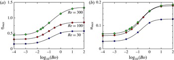
are presented in figure 4. The locations of the points in the bulk where these maximal values are attained can be discerned from the contours plots in figure 3. There is a monotonic increase in
 ${\it\eta}_{max}$
with increasing
 $Bo$
, an inflection point at
 $Bo\approx 10^{-1}$
, and
 ${\it\eta}_{max}$
asymptotes for large and small
 $Bo$
for all three
 $Re$
values. For
 $Bo\lesssim 10^{-3}$
, the flow behaves as in the limit of
 $Bo\rightarrow 0$
, while, for
 $Bo\gtrsim 10$
, the
 $Bo\rightarrow \infty$
is essentially reached. The Reynolds numbers used were selected based on the fact that experiments done in surface rheology studies using the knife-edge viscometer and aqueous systems are generally conducted in the range
 $10\lesssim Re\lesssim 10^{3}$
. For
 $Re\lesssim 30$
, previous computations have shown that the flow is in the Stokes flow regime where inertia is negligible (Lopez & Hirsa Reference Lopez and Hirsa2015). Experiments are generally avoided below this range of
 $Re$
since the signal-to-noise ratio is unacceptably small. This was also found to be the case in the present experiments, as described below. At any given
 $Bo$
, figure 4(a) also shows that
 ${\it\eta}_{max}$
increases with
 $Re$
. Figure 4(b) presents
 $u_{max}$
for various
 $Bo$
and
 $Re$
. In the Stokes flow regime,
 $u_{max}$
is proportional to
 $Re$
, and in the inertial regime
 $u_{max}$
approaches a constant value (approximately 7 % of the knife-edge velocity for small
 $Bo$
and approximately 18 % of the knife-edge velocity for large
 $Bo$
). This is the same scaling behaviour as observed in the deep-channel surface viscometer (Lopez & Hirsa Reference Lopez and Hirsa1998), which is driven by a rotating solid floor rather than a viscous film, as is the case here. The transition from viscous-dominated (Stokes flow regime) to inertia-dominated flow occurs in the same way for all
 $Bo$
. The other significance of figure 4(b) is that it shows that the secondary flow in the bulk monotonically increases with
 $Bo$
– therefore, the more viscous the film, the stronger the secondary flow. Thus, for any given
 $Re$
, the strongest bulk flow is achieved in the limit of
 $Bo\rightarrow \infty$
. The radial velocity of the bulk is less than approximately 10 % of the knife-edge speed when
 $Bo\lesssim 0.1$
, whereas the secondary flow is approximately 18 % of the knife-edge speed for
 $Bo\gtrsim 1$
and
 $Re\gtrsim 100$
.
Variation of the maximum (positive) computed azimuthal vorticity,
 ${\it\eta}_{max}$
(a), and computed radial velocity,
 $u_{max}$
(b), with
 $Bo$
for
 $Re$
as indicated.

Computed profiles of
 $v$
at various indicated depths below the surface (fraction of knife-edge radius), for
 $Re=100$
. (a)
 $Bo=10^{-3}$
; (b)
 $Bo=10^{-1}$
; (c)
 $Bo=10$
.

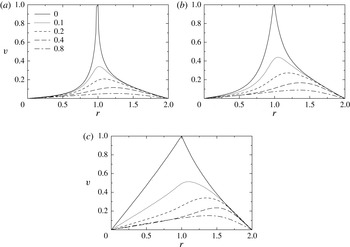
Since the PIV technique uses a finite-thickness laser light sheet, measurements cannot be made precisely at the interface. Instead, measurements are made at various depths near the interface. Numerical results presented in figure 5 provided guidance in selecting those depths; the figure shows the radial profiles of the azimuthal velocity at the interface and various depths below the interface, for the experimental geometry at
 $Re=100$
and three values of
 $Bo$
. The lowest
 $Bo=10^{-3}$
is close to that corresponding to an essentially inviscid interface, and the highest
 $Bo=10$
is close to the asymptotic regime
 $Bo\rightarrow \infty$
. The figure shows that, except for highly viscous films, velocity measurements at depths greater than approximately 20 % of the knife-edge radius will suffer from a poor signal-to-noise ratio. As such, the experimental measurements were taken with laser light sheets at nominal depths of 4 %, 10 % and 20 % of the knife-edge radius.
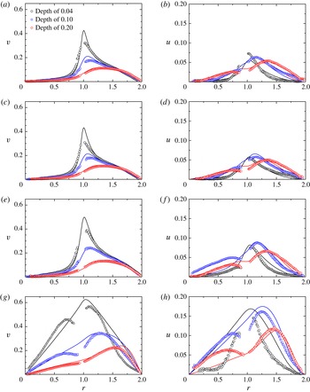
Profiles of azimuthal velocity
 $v$
(a,c,e,g) and radial velocity
 $u$
(b,d,f,h) at depths
 $0.04$
,
 $0.1$
and
 $0.2$
below the surface, for both the computed profiles (lines, at the indicated
 $Bo$
) and the experimental data (symbols, at the indicated
 ${\it\Pi}$
), at
 $Re=300$
. (a,b)
 ${\it\Pi}=5~\text{dyn}~\text{cm}^{-1}$
,
 $Bo=10^{-4}$
; (c,d)
 ${\it\Pi}=10~\text{dyn}~\text{cm}^{-1}$
,
 $Bo=10^{-3}$
; (e,f)
 ${\it\Pi}=20~\text{dyn}~\text{cm}^{-1}$
,
 $Bo=0.03$
; (g,h)
 ${\it\Pi}=40~\text{dyn}~\text{cm}^{-1}$
,
 $Bo=10$
.

Given that, for larger
 $Re$
, the signal-to-noise ratio improves, and the fact that measurements in similar geometries for surface rheological studies are conducted with
 $Re\lesssim 10^{3}$
, experiments were conducted here with
 $Re=30$
, 100 and 300. We begin by describing the results at
 $Re=300$
. For all
 $Re$
, DPPC monolayers at surface pressure
 ${\it\Pi}=5$
, 10, 20 and
 $40~\text{dyn}~\text{cm}^{-1}$
were used. At the lowest surface pressure, figure 6(a,b) shows that the monolayer is essentially inviscid. This determination was made based on comparisons between the measurements of the (primary) azimuthal velocity,
 $v$
, and computations for various values of
 $Bo$
, which showed that the best overall agreement was with
 $Bo\leqslant 10^{-4}$
(the difference between computed profiles with
 $Bo=10^{-4}$
and 0 are not discernable). For all three depths, figure 6(a,b) shows good agreement between the measurements and computations of the azimuthal velocity. The discrepancy between the measurements and the computations at the depth nearest to the interface, especially near the knife edge, may be due to a combination of the finite thickness of the light sheet and the large flow gradients in the
 $z$
-direction in that region. Furthermore, the very steep radial gradient in the flow near the interface and the knife edge challenges the spatial resolution limits of PIV measurements. At the two larger depths, the problems with measurements near the knife edge (
 $r=1$
) are not primarily due to spatial resolution limits, but rather due to the light scattered from the (stainless steel) knife edge overwhelming the light from the particles. The measurements of the radial velocity
 $u$
, presented in figure 6(b), show reasonably good agreement with the predictions. For this low surface pressure the monolayer is relatively inviscid, and the radial component of the velocity is almost an order of magnitude smaller than the azimuthal component. The settings for the PIV data acquisition were optimized for measurements of the primary flow component
 $v$
, so the greater scatter in
 $u$
, and the poorer agreement, is not unexpected. Nevertheless, figure 6(a,b) shows that the general shape of the
 $u$
profiles at all depths considered and their magnitudes are captured very well.
At a surface pressure of
 ${\it\Pi}=10~\text{dyn}~\text{cm}^{-1}$
, figure 6(c,d) shows that the monolayer is behaving slightly more viscous, yet the shape of the azimuthal velocity profile remains very similar to the
 ${\it\Pi}=5~\text{dyn}~\text{cm}^{-1}$
case. The increase in the viscosity of the interface between the
 ${\it\Pi}=5$
and
 $10~\text{dyn}~\text{cm}^{-1}$
cases is commensurate with the increase in the packing of the monolayer, i.e. a decrease in the area coverage per molecule. Figure 2 shows that the area coverage per molecule decreases from approximately 0.65 to
 $0.55~\text{nm}^{2}$
when
 ${\it\Pi}$
is increased from 5 to
 $10~\text{dyn}~\text{cm}^{-1}$
. In figure 6(c,d), we have shown the computed profiles at
 $Bo=10^{-3}$
, although the computed profiles at
 $Bo=10^{-3}$
and
 $Bo=10^{-4}$
differ by approximately the same amount as the scatter in the measured data. So, at
 ${\it\Pi}=10~\text{dyn}~\text{cm}^{-1}$
the monolayer is nearly inviscid. The magnitude of
 $u$
is a little smaller at the larger
 ${\it\Pi}$
, which is counter to what one would expect. However, this discrepancy is within the experimental uncertainty, and laser light heating issues also contribute (this is addressed in detail below).
For a monolayer with a surface pressure of
 $20~\text{dyn}~\text{cm}^{-1}$
, figure 6(e,f) shows a noticeable increase in both
 $v$
and
 $u$
at all three depths. Although
 ${\it\Pi}$
is double that of the case in figure 6(c,d), the surface packing is only slightly larger. The agreement between the measurements and the predictions for this case is excellent. This is likely due to the larger velocity signal (higher signal-to-noise ratio) associated with the more viscous interface. It should be noted that, at this surface pressure, DPPC is still a fluid monolayer and the packing is not large enough to produce a solid-phase film (McConnell Reference McConnell1991).
At the largest surface pressure considered,
 ${\it\Pi}=40~\text{dyn}~\text{cm}^{-1}$
, shown in figure 6(g,h), the monolayer is significantly more viscous, and so the driven bulk flow is faster. Although this results in an even better signal-to-noise ratio, the discrepancy between measured and predicted profiles is markedly worse. Trying to match the profiles with a single value of
 $Bo$
for this high
 ${\it\Pi}$
case does not work well. The fit used is with
 $Bo=10$
, but for
 $0<r<1$
(inside the knife edge) this is too small (a larger
 $Bo$
would drive a faster flow, see figures 4 and 5), whereas for
 $1<r<2$
(outside the knife edge)
 $Bo=10$
is too large to fit the measurements. This means that the Newtonian interfacial model used does not describe the flow of the highly packed monolayer at
 ${\it\Pi}=40~\text{dyn}~\text{cm}^{-1}$
. This is not surprising as, at this surface pressure, DPPC is known to be in a solid phase at room temperature (McConnell Reference McConnell1991).
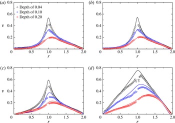
Measurements and comparisons with predictions at
 $Re=100$
are presented in figure 7. Only the primary azimuthal velocity component
 $v$
is presented because, at this lower
 $Re$
, the radial velocity
 $u$
is smaller and becomes comparable to the noise in the measurements. For
 ${\it\Pi}=5$
and
 $10~\text{dyn}~\text{cm}^{-1}$
, there is excellent agreement between model and experiments. The monolayer is essentially inviscid for
 ${\it\Pi}=5~\text{dyn}~\text{cm}^{-1}$
and very slightly viscous for
 ${\it\Pi}=10~\text{dyn}~\text{cm}^{-1}$
, consistent with the higher
 $Re=300$
results. For
 ${\it\Pi}=20~\text{dyn}~\text{cm}^{-1}$
, this more densely packed film is best fitted with
 $Bo=0.01$
, which is smaller than the
 $Bo=0.03$
used for the same monolayer at
 $Re=300$
. Interestingly, for the highest surface pressure
 ${\it\Pi}=40~\text{dyn}~\text{cm}^{-1}$
the fit with
 $Bo=10$
(as was used for the
 $Re=300$
case) is very good, and surprisingly it fits better than in the
 $Re=300$
case, even though the signal-to-noise ratio of the velocity measurements is lower.
Profiles of azimuthal velocity
 $v$
at depths
 $0.04$
,
 $0.1$
and
 $0.2$
below the surface, for both the computed profiles (lines, at the indicated
 $Bo$
) and the experimental data (symbols, at the indicated
 ${\it\Pi}$
), at
 $Re=100$
. (a)
 ${\it\Pi}=5~\text{dyn}~\text{cm}^{-1}$
,
 $Bo=10^{-4}$
; (b)
 ${\it\Pi}=10~\text{dyn}~\text{cm}^{-1}$
,
 $Bo=10^{-3}$
; (c)
 ${\it\Pi}=20~\text{dyn}~\text{cm}^{-1}$
,
 $Bo=0.01$
; (d)
 ${\it\Pi}=40~\text{dyn}~\text{cm}^{-1}$
,
 $Bo=10$
.

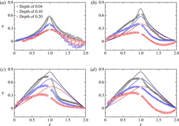
Profiles of azimuthal velocity
 $v$
at depths
 $0.04$
,
 $0.1$
and
 $0.2$
below the surface, for both the computed profiles (lines, at the indicated
 $Bo$
) and the experimental data (symbols, at the indicated
 ${\it\Pi}$
), at
 $Re=30$
. (a)
 ${\it\Pi}=5~\text{dyn}~\text{cm}^{-1}$
,
 $Bo=10^{-4}$
; (b)
 ${\it\Pi}=10~\text{dyn}~\text{cm}^{-1}$
,
 $Bo=0.1$
; (c)
 ${\it\Pi}=20~\text{dyn}~\text{cm}^{-1}$
,
 $Bo=10$
; (d)
 ${\it\Pi}=40~\text{dyn}~\text{cm}^{-1}$
,
 $Bo=100$
.

Measurements at the lowest
 $Re=30$
, presented in figure 8, reveal a significant amount of noise, especially outside of the knife edge. Although the best fits to the measurements at each surface pressure were conducted and presented in the figure, the intrusiveness of the laser light sheet appears to have overwhelmed the signal at this low
 $Re$
, and the values of
 $Bo$
quoted should be taken with a grain of salt. In particular, at large radial distances, the mean azimuthal velocity is negative in many cases. This is not possible if the flow were solely driven by the rotating knife edge and the viscous traction of the monolayer. In order to understand where this extraneous flow is coming from, we conducted two control experiments consisting of velocity measurements made at the same three depths but with the knife edge stationary, i.e. with
 $Re=0$
. In one case with a clean free surface (no monolayer deposited) and the other with a monolayer of DPPC at
 ${\it\Pi}=40~\text{dyn}~\text{cm}^{-1}$
. In both cases, large-scale recirculations were observed, with velocities at each of the three depths of approximately
 $0.2~\text{mm}~\text{s}^{-1}$
. For the
 $Re=30$
cases, this amounts to approximately 10 % of the knife-edge velocity, for
 $Re=100$
it is approximately 3 %, and for
 $Re=300$
it is 1 % of the knife-edge velocity, which is comparable to PIV measurement uncertainty.
4. Discussion and conclusions
Our results show that a strong bulk flow can be driven by a viscous monolayer, comparable to that on a rotating solid endwall. At any given Reynolds number, the more viscous the interface, the stronger the bulk flow; this was numerically predicted in Lopez & Hirsa (Reference Lopez and Hirsa2015) and has now been verified experimentally. Even at small
 $Re$
, when the surface is viscous the magnitude of the secondary flow is 10 % of the knife-edge speed, so that secondary meridional flows are not negligible even in the Stokes flow limit. While most treatments of interfacial flows driven by knife edges or needles neglect the secondary bulk flow, the possible importance of the coupling between the interfacial and bulk flows is well recognized (Slattery et al.
Reference Slattery, Sagis and Oh2007; Langevin Reference Langevin2014b
).
The direct experimental measurements presented here show that a significant secondary meridional bulk flow can be driven by a viscous monolayer. Secondary meridional flow is important in part because it plays a crucial role in the distribution of the vortex lines in the bulk and, in turn, in where and how they meet the interface. This then determines the shear strain distribution at the interface. The shear strain distribution is generally used to interpret the viscous response of the surface film and deduce its surface shear viscosity. So, unless the bulk flow coupling is accounted for, the interfacial hydrodynamics is inaccurate except in the limit of
 $Bo\rightarrow \infty$
. For a given system, with a given bulk and interfacial viscosity, this limit requires the length scale to vanish. However, such limits are not necessary in order to accurately characterize the interfacial hydrodynamics. In fact, designing a knife-edge apparatus with a length scale to achieve
 $Bo\sim 0.1$
increases the sensitivity of the flow as a surface shear viscometer. For
 $Bo$
much larger or smaller than approximately 0.1, an order of magnitude variation in
 $Bo$
only results in approximately a 1 % variation in the flow velocity.
The primary focus of the present study was to explore the extent to which bulk fluid is driven by the motion of a viscous monolayer. We selected a flow geometry which was originally designed to measure the surface shear viscosity of interfacial films. Measuring surface shear viscosity was not the objective, but came as a byproduct of the study. The length scale of the present experiments (knife-edge diameter
 $2a=2.54~\text{cm}$
) was selected in order to have the largest possible precision glass cylinder readily available and therefore minimize the relative error due to geometric imperfections. This scale also affords the availability of suitable seeding particles that are small (a few microns) compared to the length scale of the apparatus. With this length scale, the knife-edge viscometer gives
 $Bo$
values that are very small for DPPC at small surface pressures (
 $Bo\lesssim 10^{-3}$
for
 ${\it\Pi}\lesssim 10~\text{dyn}~\text{cm}^{-1}$
), and for large surface pressure of
 ${\it\Pi}=40~\text{dyn}~\text{cm}^{-1}$
the DPPC film exhibits a very viscous response since it is known to be in a solid phase, and additional physics is involved. For intermediate
 ${\it\Pi}=20~\text{dyn}~\text{cm}^{-1}$
,
 $Bo$
is closer to the desirable range, but it appears to be
 $Re$
-dependent, probably due to the complex phase of the DPPC film at that surface pressure. This all translates into the following dimensional surface shear viscosity values for DPPC: for
 ${\it\Pi}=5~\text{dyn}~\text{cm}^{-1}$
,
 ${\it\mu}^{s}\sim 10^{-3}~\text{mg}~\text{s}^{-1}$
; for
 ${\it\Pi}=10~\text{dyn}~\text{cm}^{-1}$
,
 ${\it\mu}^{s}\sim 10^{-2}~\text{mg}~\text{s}^{-1}$
; for
 ${\it\Pi}=20~\text{dyn}~\text{cm}^{-1}$
,
 ${\it\mu}^{s}\sim 0.1~\text{mg}~\text{s}^{-1}$
for
 $Re=100$
and
 ${\it\mu}^{s}\sim 0.3~\text{mg}~\text{s}^{-1}$
for
 $Re=300$
; and for
 ${\it\Pi}=40~\text{dyn}~\text{cm}^{-1}$
,
 ${\it\mu}^{s}\sim 10^{2}~\text{mg}~\text{s}^{-1}$
. What is evident is that DPPC over the range of surface pressures of interest (over which it forms a monomolecular film on the surface of water) has a very large range of surface shear viscosity, and in order to measure it with some precision requires a number of knife-edge viscometers with a commensurate range of scales. This is not unique to interfacial viscometry. For example, a capillary viscometer, with a given diameter, for determining dynamic viscosity
 ${\it\mu}$
typically covers only a fraction of one decade of dynamic range.
We used the most accurate modelling of axisymmetric flow in the bulk via the Navier–Stokes equations, and for the interface we used the Boussinesq–Scriven surface model, which treats the interface as Newtonian. This simplest model for the interface captures the interfacial hydrodynamics of DPPC well for surface pressures up to approximately
 $20~\text{dyn}~\text{cm}^{-1}$
. Note that this is approximately half the surface pressure at which a quiescent film of DPPC collapses (McConnell Reference McConnell1991). For surface pressures above
 $20~\text{dyn}~\text{cm}^{-1}$
, there are regimes where the DPPC film is known to be in condensed liquid as well as solid phases (McConnell Reference McConnell1991). In these regimes, the Boussinesq–Scriven surface model does not give shear-independent results, i.e. the effective surface shear viscosity varies with Reynolds number, and the general shapes of the velocity profiles differ between the model and the experimental measurements. Similar results were obtain in a deep-channel viscometer (Sadoughi, Lopez & Hirsa Reference Sadoughi, Lopez and Hirsa2013). Note that, in the deep-channel viscometer, the interfacial flow is solely driven by the bulk flow, whereas in the knife-edge geometry, the interface is primarily driven by the moving knife edge, and the bulk flow is driven by the surface film, which is also impacted upon by the bulk flow. In the deep-channel, the transition away from Newtonian interfacial behaviour was observed to occur at surface pressures of approximately
 $15~\text{dyn}~\text{cm}^{-1}$
. The difference in the transition surface pressure between the two flow geometries may be attributable to differences in both the magnitude and distribution of the shear rate at the interface. The present measurements at the maximum surface pressure of
 ${\it\Pi}=40~\text{dyn}~\text{cm}^{-1}$
show that inside the knife edge, where the film is not strongly sheared and flows essentially like a solid body, the apparent viscosity is large, while outside the knife edge the film is strongly sheared and exhibits shear thinning. In the deep-channel geometry, Sadoughi et al. (Reference Sadoughi, Lopez and Hirsa2013) also concluded that DPPC films at high surface pressure are shear thinning, based on their measurements showing surface shear viscosity decreasing with increasing Reynolds number.
In order to improve the accuracy of the interfacial model for the solid phase of the film, the Boussinesq–Scriven surface model should be generalized in order to account for a nonlinear relation for interfacial stress and rate of strain.
Acknowledgements
This work was supported by NASA grant NNX13AQ22G and the National Science Foundation grants CBET-1064644 and CBET-1064498. We thank C. F. Tilger for assistance in the design and fabrication of the flow apparatus.
Appendix. Preparation of DPPC monolayers
The structure and behaviour of insoluble films spread on the surface of water, which are often monomolecular, depend on the process used to spread the film. In the field of physical chemistry of surfaces, practitioners have developed techniques that are adopted widely (see monogram by Gaines Reference Gaines1966). However, in this respect the fluid dynamics literature is terse and details are not given, making quantitative comparisons of monolayer hydrodynamics scarce. Here we provide the details of the technique utilized for the handling and formation of DPPC monolayers.
Sealed glass ampoules of DPPC with a purity of better than 99 % and dissolved in chloroform were purchased (Avanti Polar Lipid; 850355C, 25 mg,
 $10~\text{mg}~\text{ml}^{-1}$
) and kept in a freezer (
 $-20\,^{\circ }\text{C}$
). An ampoule was removed from the freezer and allowed to reach room temperature so that any DPPC that precipitates while in cold storage has a chance to redissolve in chloroform. The neck of the ampoule was then snapped off and
 $100~{\rm\mu}\text{l}$
of stock solution was withdrawn with a gas-tight glass syringe and a stainless steel needle with a flat (
 $90^{\circ }$
) tip and diluted with 4 ml of HPLC-grade chloroform in a previously cleaned 8 ml glass vial with a PTFE lined cap. Analytical-standard argon from an aerosol can (Sigma Aldrich; 501247) was gently sprayed into the vial to protect DPPC against oxidation every time prior to capping the vial. After the vials were capped, they were stored in the freezer. Four hours prior to each experiment, a vial was removed from the freezer and allowed to reach room temperature before uncapping and withdrawing the monolayer-forming solution. It was found that a maximum of 10 vials could be prepared from a single
 $10~\text{mg}~\text{ml}^{-1}$
stock solution ampoule, with minimal evaporative losses, consistently achieving the required solution concentration to an accuracy of 98 %. We also found that the number of times that a vial could be uncapped and capped to extract some solution was no more than three times before the errors in concentration became unacceptably large. The error in the solution concentration was determined by comparing the expected weight and the measured weight of the vial. The vials were weighed on an analytical balance with a resolution of 0.01 mg, after they had reached room temperature and any condensation on the outside of the vial had evaporated.
A Langmuir trough was used for the measurements of the equation of state, as described elsewhere (Vogel & Hirsa Reference Vogel and Hirsa2002). For these measurements, the monolayer was spread as follows:
 $100~{\rm\mu}\text{l}$
of chloroform–DPPC solution was withdrawn using a
 $250~{\rm\mu}\text{l}$
gas-tight glass syringe with a 22 gauge stainless steel, standard sharp point needle (
 $22^{\circ }$
bevel with a slightly bent tip), and was then deposited on the surface of freshly prepared DI water in the Langmuir trough. With the desired volume of DPPC in chloroform solution, the syringe was brought towards the surface, droplets (approximately
 $10~{\rm\mu}\text{l}$
in volume) were formed at the tip of the needle (held at approximately
 $30^{\circ }$
to the surface), and then the syringe was gradually lowered to facilitate contact between the droplet and the surface of water. Upon contact, the surface of water grabs the pendant drop from the syringe needle and rapidly spreads the solution on the air–water interface. Subsequently, chloroform, which has very low solubility in water, evaporates from the interface, leaving behind a monolayer of DPPC. Because of the high vapour pressure of chloroform, it is vital that the droplets are grown only when the tip of the syringe is held approximately 3–4 mm above the water surface. This minimizes chloroform evaporation from the droplet, as transfer to the surface of water is imminent, ensuring accuracy of the volume delivered to the interface, and minimizing any drying of DPPC on the needle tip. Droplets of monolayer-forming solution were deposited at various locations on the surface of the trough to ensure a homogeneous film. The monolayer was allowed to equilibrate for approximately 20 min before measurements were performed.
For the experiments in the flow apparatus (glass dish), the monolayer-forming solution was spread using a
 $25~{\rm\mu}\text{l}$
gas-tight syringe, also with a 22 gauge stainless steel, standard sharp point. The volume deposited was calculated based on the area of the glass cylinder and the desired surface pressure using the equation of state. The accuracy of the surface pressure was independently verified on an identical glass dish, but without a knife-edge assembly atop of it, so that surface tension could be directly measured with a Wilhelmy plate and an electrobalance.