
1. Introduction
The behaviour of granular media in a silo is a ubiquitous problem arising in various industrial applications (de Gennes Reference de Gennes1999). When a silo opening is large compared with the grain size, the material flows out continuously and the quasi-steady movement inside the silo appears to be relatively well captured by local constitutive theories, particularly the  $\mu (I)$-rheology, which relates the ratio of shear stress and pressure,
 $\mu$, to the dimensionless shear rate,
 $I$ (Jop, Forterre & Pouliquen Reference Jop, Forterre and Pouliquen2006; Kamrin Reference Kamrin2010; Staron, Lagrée & Popinet Reference Staron, Lagrée and Popinet2012; Dunatunga & Kamrin Reference Dunatunga and Kamrin2015). However, contrary to local constitutive theories, which lack an intrinsic size scale, it is well known that silos can arrest even when the opening is still a finite size (Beverloo, Leniger & van de Velde Reference Beverloo, Leniger and van de Velde1961; Zuriguel et al. Reference Zuriguel, Pugnaloni, Garcimartín and Maza2003; Choi, Kudrolli & Bazant Reference Choi, Kudrolli and Bazant2005; Sheldon & Durian Reference Sheldon and Durian2010; Thomas & Durian Reference Thomas and Durian2013). This behaviour occurs when the opening size is a small multiple of the grain size, and is characterized by the formation of an arch-shaped bridge of grains that spans the opening. While the phenomenon of silo clogging can be modelled well using grain-by-grain discrete element method (DEM) simulations (e.g. Martin et al. Reference Martin, Dubois, Monerie and Radjai2009; Hidalgo et al. Reference Hidalgo, Lozano, Zuriguel and Garcimartín2013), this approach becomes computationally expensive for large systems. Upscaled relations that have been proposed to capture silo arrest include the well-known Beverloo correlation, an empirical formula that models the outflow rate from a silo directly in terms of the difference between the opening size and a multiple of the grain size (Beverloo et al. Reference Beverloo, Leniger and van de Velde1961). A blockage criterion is obtained by setting the Beverloo outflow to zero. Engineering tools exist such as the Jenike method (Jenike Reference Jenike1964) to design silos and chutes that always support flow. Another theory for silo clogging reconciles the effect as due to the opening being too small for a finite-sized ‘spot’ of localized motion to pass through (Bazant Reference Bazant2006; Rycroft et al. Reference Rycroft, Bazant, Grest and Landry2006). While hybridized DEM–continuum simulations can produce flow stoppage as long as the material near the opening is treated with DEM (Yue et al. Reference Yue, Smith, Chen, Chantharayukhonthorn, Kamrin and Grinspun2018), to our knowledge, no fully continuum constitutive model has been shown capable of capturing the stoppage behaviour of non-cohesive grains in silos.
It is the goal of the current work to present such an analysis. The particular model we shall consider is the non-local granular fluidity (NGF) model, which has been shown to capture a variety of non-local effects in granular media (Kamrin & Koval Reference Kamrin and Koval2012; Henann & Kamrin Reference Henann and Kamrin2014; Kamrin Reference Kamrin2019, Reference Kamrin2020). When we say non-local, we use the term loosely to refer to a continuum model that includes an explicit length scale within the rheology, which will be detailed below. Importantly, NGF has been shown to accurately predict size-dependent flow thresholds in a range of quasi-one-dimensional geometries (Kamrin & Henann Reference Kamrin and Henann2015; Liu & Henann Reference Liu and Henann2018), which encourages its usage for predicting opening-size dependence in silo arrest. As long as our study is restricted to simple granular media (i.e. spherical particles), we also know a priori the model calibration, which enables a more stringent test. The methodology shown herein extends on the initial work on continuum silo modelling using NGF in the author's thesis (Dunatunga Reference Dunatunga2017).
It is worth noting that quantifying silo clogging (and flow thresholds in general) is non-trivial. As the opening size is reduced, flow intermittency occurs, which can cause one silo realization to clog even though other realizations may continue to flow (Sheldon & Durian Reference Sheldon and Durian2010; Thomas & Durian Reference Thomas and Durian2013, Reference Thomas and Durian2016). Many studies have been conducted to quantify the statistics and scalings of particle release events in the intermittent range (To, Lai & Pak Reference To, Lai and Pak2001; Zuriguel et al. Reference Zuriguel, Garcimartín, Maza, Pugnaloni and Pastor2005, Reference Zuriguel2014). Interestingly, it was shown in Thomas & Durian (Reference Thomas and Durian2013) that, while a silo may first clog at one opening size, the critical opening size at which all silos clog is often much smaller and corresponds well with the apparent flow cutoff obtained from extrapolating the Beverloo correlation. In comparing with a continuum model, our belief is that the continuum solution should predict when the ensemble-averaged flow rate vanishes, which corresponds to this critical size just described.
2. NGF model
The NGF model was originally developed as a means to include a length scale within an otherwise local rheology for steady granular flow. A local rheology is taken to be a constitutive relation in which the local flow state is directly obtainable from the local stress state (and any locally evolving state fields). The NGF model was initially proposed as a means to reconcile observed departures from the  $\mu (I)$ relation in inhomogeneous steady flow geometries, most pronounced when
 $I$ is small, such as annular shear flows and vertical chute flows. It was later observed that the dynamic form of the NGF model is also able to determine grain-size dependent flow threshold criteria, i.e. when flow in a geometry ceases due to a certain feature of the geometry becoming a small multiple of the mean grain size. In this regard, the NGF model quantitatively predicts the threshold thickness for flow stoppage of spherical grains down inclined chutes (Kamrin & Henann Reference Kamrin and Henann2015). Similarly, NGF predicts flow arrest in two-dimensional (2-D) cases of disks under annular shear loading, gravity-driven vertical chute flow, and shear load combined with gravity (Liu & Henann Reference Liu and Henann2018).
The dynamic (primitive) form of the NGF model can be expressed as an evolution rule for a phase field,  $g(x)$, referred to as the ‘granular fluidity’
 \begin{equation} t_0\dot{g}=A^{2}d^{2}\nabla^{2}g-\varDelta_\mu \left( \frac{\mu_s-\mu}{\mu_2-\mu} \right)g -b\sqrt{\frac{\rho_s d^{2}}{p}}\mu g^{2}, \end{equation}
where  $\dot {g}$ is the material time rate of change of the fluidity
 $g$, A the ‘non-local amplitude’,
 $d$ is the mean grain size,
 $\rho _s$ is the solid grain density,
 $t_0$ is a time scale, p the pressure,
 $\tau$ the shear stress,
 $\mu _s$ and
 $\mu _2$ are the lower and upper bounds taken by the stress ratio
 $\tau /p\equiv \mu$ during flow,
 $\varDelta _\mu =\mu _2-\mu _s$ and
 $b$ is a material constant equal to
 $\varDelta _\mu / I_0$ (
 $I_0$ is the same material constant as used in the
 $\mu (I)$ rheology). The solid grain density
 $\rho _s$ is related to the continuum granular bulk density
 $\rho$ via
 $\rho = \rho _s \varPhi$, where
 $\varPhi$ is the packing fraction. The constitutive relation then calls upon the
 $g$ field to relate stress and strain rate via
 \begin{equation} \dot{\gamma}=g\mu. \end{equation}
The  $A^{2}d^{2}\nabla ^{2}g$ term in the evolution of
 $g$ implies that the spatial diffusion of the fluidity field is influenced directly by the mean particle size. Hence, flow at a point is not given solely by stress at that point, but rather is influenced by nearby events through the
 $g$ field. At steady state, the non-local amplitude
 $A$ is the only new material parameter affecting the flow solution beyond those of the inertial rheology. If
 $A$ is set to
 $0$ in the limit of vanishingly small
 $t_0$, the steady solutions of the system reduce identically to the inertial
 $\mu (I)$ rheology. Here,
 $A$ is dimensionless and order one;
 $A\approx 0.5$ for glass beads and
 $\approx 0.9$ for stiff DEM disks (Henann & Kamrin Reference Henann and Kamrin2013; Kamrin & Koval Reference Kamrin and Koval2014). Provided with boundary conditions on the fluidity, the velocity and the stress via tractions, the above becomes a complete constitutive relation. Both Dirichlet and Neumann boundary conditions on the fluidity are considered here and will be explored more deeply in each scenario. As done in prior work, the model can be extended directly to three dimensions by defining
 $\mu$ and
 $\dot {\gamma }$ based on tensorial invariants (Henann & Kamrin Reference Henann and Kamrin2013).
3. Grain-size-dependent flow thresholds from non-local rheology
To explain how size-dependent thresholds arise in NGF, it is instructive to consider first a paradigmical case, which will be used later for code validation. In recent years, the size dependence of the flow threshold for flow down an inclined chute has come to be a famous example of non-locality in granular flow (Pouliquen Reference Pouliquen1999). In brief, while local models would predict a thickness-independent repose angle, many experiments show (MiDi Reference MiDi2004) that the angle at which a flowing layer arrests grows as the thickness of the layer reduces, and the critical thickness as a function of tilt is known as  $H_{{stop}}(\theta )$. See figure 2 for geometry details. One can show from symmetry and quasi-static balance that in the inclined chute,
 $\mu =\tan \theta$ and
 $p=zg\cos \theta$ where
 $z$ measures depth orthogonal to the free surface and
 $\theta$ is the incline angle from the horizontal. Also, from previous data (Silbert, Landry & Grest Reference Silbert, Landry and Grest2003), we can infer that the boundary conditions for the
 $g$ field are approximately
 $\partial _n g = 0$ at
 $z=0$ (the free surface) and
 $g(z=H)=0$ (the base).
Unlike local models, the NGF model predicts an  $H_{{stop}}$ curve for this geometry (Kamrin & Henann Reference Kamrin and Henann2015), which arises due to (2.1) developing a bifurcation that causes the
 $g=0$ solution to lose stability. That is, while
 $g=0$, i.e. no flow, is always a solution to the NGF partial differential equation (PDE), it is not always a stable solution. Note also that there is no hysteresis in the NGF model used here, so
 $H_{{stop}}$ is the same as
 $H_{{start}}$ (which relates the layer height to tilt angle at flow initiation instead of flow stoppage), a fact we will make use of in verification. A linear stability analysis of the PDE in the case of an inclined chute reveals that the stability of the global
 $g=0$ solution is lost when
 \begin{equation} \frac{H}{d}>\frac{{\rm \pi} A }{2} \sqrt{\frac{\mu_2-\tan\theta}{\varDelta_\mu(\tan\theta-\mu_s)}} \equiv H_{{stop}}(\theta). \end{equation}
We see the right-hand side defines the  $H_{{stop}}(\theta )$ function. Experiments with glass beads produce an
 $H_{{stop}}$ curve that is close to the solution above when calibrated to the (known) NGF parameters for glass beads. Outside of tilted chutes, the ability of NGF to capture size-dependent flow thresholds was validated in a number of 2-D geometries as well, where, just as in the inclined flow case, an analytical solution for the stoppage criterion was found in each case, which predicted the DEM stoppage data to a quantitative level (Liu & Henann Reference Liu and Henann2018).
Clogging of a silo opening shares many similarities with the size-dependent stoppage effect described above. Most saliently, it is a phenomenon that occurs when the width of the flow domain – i.e. the silo opening – competes on the scale of the grain size. The fact that the grain size is the key length scale implies any continuum treatment would need to be non-local to represent this effect. As such, we seek to determine if the NGF model is capable of predicting silo clogging.
4. Modelling details for implementing general flow cases
The NGF equation shown in (2.1) is intended for dense granular flows. To use NGF in the silo configuration, the model must be augmented in order to represent separated material. This disconnected granular phase occurs in the stream of grains that exits a silo when it is flowing, or the material that falls out underneath the arch that bridges the opening when a silo clogs. Without adding a representation of the disconnected phase, determining if a silo clogs for a given opening size would be difficult. One would have to guess an arch shape first and then check if the configuration stays static by seeing if an initially perturbed  $g$ field evolves to approach zero everywhere. Even if the vanishing
 $g$ solution were stable, it would be unclear if the chosen arch shape were correct – would the system have found the same arch naturally upon opening a full silo? Indeed, the arch that forms when a silo clogs should be an emergent geometric outcome and not an input.
In order to properly simulate the formation, or lack thereof, of a stable arch, we extend the NGF model to permit a disconnected phase using a framework similar to that used in Dunatunga & Kamrin (Reference Dunatunga and Kamrin2015), which conjoined a separation rule with the local inertial rheology. As in that work, we consider for simplicity that the disconnected phase is stress free and defined by when the density,  $\rho$, is less than some critical value,
 $\rho _c$. The dense phase, which abides by the NGF equation, is approximated to be plastically incompressible and defined by
 $\rho =\rho _c$. The density field is obtained by enforcing mass conservation throughout the domain.
On the interface between dense and disconnected phases, the  $g$ field requires a boundary condition. We enforce the Neumann condition
 $\partial _n g=0$ on these interfaces, guided by our previous observations and prior usage of the Neumann condition along granular free surfaces (Silbert et al. Reference Silbert, Landry and Grest2003; Kamrin & Henann Reference Kamrin and Henann2015). In the event that a zone of granular media reconsolidates from a previously disconnected state, an uncommon event in a silo flow, we want a physically consistent way to re-initialize the
 $g$ variable. This resembles the ‘Stefan free-boundary problem’, frequently encountered in the modelling of solid/liquid fronts in a melting or freezing material specimen. While the classical Stefan problem involves setting multiple boundary conditions for the temperature on a phase front defined by the temperature itself, in our case the question is slightly different in that we must decide boundary conditions for
 $g$ on consolidation interfaces, which are themselves defined by
 $\rho$. In the results below, we choose to set
 $g=0$ in newly reconsolidated material, which is the value of
 $g$ the steady inertial rheology would assume if a finite stress state is uniformly scaled down to zero. Another option for reinitializing
 $g$ was used in Dunatunga (Reference Dunatunga2017) but we noticed it did not make a significant difference in our reported results when we tried it.
4.1. Generalizing to an elasto-plastic framework
To accurately implement a model with the components described – allowing for the possibility of stopped material with an apparent yield stress, dense flow obeying a non-local rheology, and separation/reconsolidation of material – is a very challenging task. We have chosen to address these challenges by representing the model in an elasto-plastic framework, with details provided next. This approach, which we have used previously for a purely local material model (Dunatunga & Kamrin Reference Dunatunga and Kamrin2015), essentially turns our proposed rheology into a complex Maxwell fluid by putting the flow rule in series with an elastic element (a ‘spring’) whose stiffness vanishes when the material density drops below  $\rho _c$. As long as the spring is stiff in the dense (positive pressure) regime, its effect on the flow is negligible. However, its presence not only assists in implementing the separation/reconsolidation rule, but allows us to model the onset of a true yield stress without the need for viscous regularization.
4.2. Summary of equations
We use the standard notation for continuum mechanics as defined in Gurtin, Fried & Anand (Reference Gurtin, Fried and Anand2010). The trace of a tensor  $\boldsymbol {A}$ is given by
 $\operatorname {tr} \boldsymbol {A}$, the transpose by
 $\boldsymbol {A}^{\rm T}$, the inverse by
 $\boldsymbol {A}^{-1}$ and the deviator by
 $\boldsymbol {A}_0 = \boldsymbol {A} - \frac {1}{3} (\operatorname {tr} \boldsymbol {A}) \boldsymbol {I}$ in three dimensions. Scalars are represented by lowercase text, points and vectors by lowercase bold text and tensors are represented by uppercase bold text (except the Cauchy stress is
 $\boldsymbol {\sigma }$). The dot product over vectors is represented with a single centred dot, and simply multiplies the vectors together componentwise and takes the sum, resulting in a scalar (e.g.
 $\boldsymbol {a} \boldsymbol {\cdot } \boldsymbol {b} = \sum _{i} a_i b_i$). Tensorial contraction is represented with a colon, and multiplies tensors together componentwise and takes the sum, also resulting in a scalar (e.g.
 $\boldsymbol {A} \colon \boldsymbol {B} = \sum _{i,j} A_{ij} B_{ij}$). The spatial gradient and spatial divergence operators are given by
 $\operatorname {grad}$ and
 $\operatorname {div}$ respectively. Overdots indicate a material time rate of change of the underlying variable.
Define the strain-rate tensor  $\boldsymbol {D}=(\boldsymbol {\nabla }\boldsymbol {v}+\boldsymbol {\nabla }\boldsymbol {v}^{\rm T})/2$ and the spin (vorticity) tensor
 $\boldsymbol {W}=(\boldsymbol {\nabla }\boldsymbol {v}-\boldsymbol {\nabla }\boldsymbol {v}^{\rm T})/2$ from the velocity field
 $\boldsymbol {v}$. From the stress tensor, define the equivalent shear stress
 $\bar {\tau }=\sqrt {\sum _{i,j}\sigma _{0 ij}\sigma _{0 ij}/2}$ and hydrostatic pressure
 $p=-(1/3)\sum _i\sigma _{ii}$, which are used to define the stress ratio
 $\mu =\bar {\tau }/p$. Let the specific body force (here from gravity) be denoted
 $\boldsymbol {b}$, the plastic part of the strain rate be denoted
 $\boldsymbol {D}^{p}$ (and elastic part
 $\boldsymbol {D}^{e}\equiv \boldsymbol {D}-\boldsymbol {D}^{p}$) and the shear and bulk elastic moduli be denoted
 $G$ and
 $K$.
With these definitions in hand, let  $\varOmega$ be the material domain, let
 $\varOmega _d$ represent the subdomain where material is dense (
 $\rho >\rho _c$) and let
 $\varOmega _s$ represent the subdomain where material is separated (
 $\rho <\rho _c$). The continuum system we solve is summarized as follows:
For all  $\boldsymbol {x}\in \varOmega$
(i) Balance of linear momentum, angular momentum and mass
(4.1a–c) \begin{equation} \operatorname{div} \boldsymbol{\sigma} + \rho \boldsymbol{b} = \rho \dot{\boldsymbol{v}},\quad \boldsymbol{\sigma} = \boldsymbol{\sigma}^{\rm T},\quad \dot{\rho}={-}\rho\operatorname{div} \boldsymbol{v}. \end{equation}

For all  $\boldsymbol {x}\in \varOmega _d$
(i) Elasticity relation
(4.2)\begin{equation} \dot{\boldsymbol{\sigma}}-\boldsymbol{W}\boldsymbol{\sigma}+ \boldsymbol{\sigma}\boldsymbol{W} =K \operatorname{tr} (\boldsymbol{D}-\boldsymbol{D}^{p}) \boldsymbol{1}+2G(\boldsymbol{D}-\boldsymbol{D}^{p})_0. \end{equation}(ii) Plastic flow rule
(4.3)\begin{equation} \dot{\bar{\gamma}}^{p}\equiv \sqrt{\sum_{i,j}2D_{ij}^{p}D_{ij}^{p}}=g\mu,\quad \boldsymbol{D}^{p}=\dot{\bar{\gamma}}^{p}\frac{\boldsymbol{\sigma}_0}{2\tau}. \end{equation}(iii) Non-local fluidity PDE
(4.4)\begin{equation} t_0\dot{g}=A^{2}d^{2}\nabla^{2}g-\varDelta_\mu \left( \frac{\mu_s-\mu}{\mu_2-\mu} \right)g -b\sqrt{\frac{\rho_s d^{2}}{p}}\mu g^{2}. \end{equation}


For all  $\boldsymbol {x}\in \varOmega _s$
(i) Open material condition:
(4.5)\begin{equation} \boldsymbol{\sigma}=\boldsymbol{0}. \end{equation}

The above equations are solved simultaneously with the aforementioned (re)consolidation rule for material passing through  $\rho =\rho _c$ and appropriate boundary conditions for
 $g$, tractions and velocities on walls and free surfaces. Note that, although the mathematical model is fully three-dimensional, our simulations employ 2-D plane-strain assumptions (that is,
 $D_{zz} = 0$, but
 $\sigma _{zz} \ne 0$) in our implementation to reduce unnecessary computations.
We would like to emphasize that we are primarily interested in solutions where the elastic moduli are high (correspondingly, the elastic time scale is small) and the fluidity time scale  $t_0$ is low. The fluidity time scale
 $t_0$ is a real parameter of the model, but at present we have no experimental data to calibrate it, so we choose a low value for convenience. A low value of
 $t_0$ implies that the steady-state solution for
 $g$ is achieved much faster than the geometry of the system changes. This ensures that the system quickly determines if
 $g = 0$ (the clogged case) is the stable solution, or if a flowing
 $g \ne 0$ solution prevails. The
 $t_0 \dot {g}$ term is important, even if
 $t_0$ is small, as it allows the system to determine the stable solution on its own by advancing forward in time – if we remove the term entirely, giving a steady-state form, we would need to perform a perturbation analysis to determine which solution is the stable one (this is difficult for general geometries).
5. Numerical solution: material point method
5.1. Introduction
The material point method (MPM), developed in Sulsky, Chen & Schreyer (Reference Sulsky, Chen and Schreyer1994), sits at the intersection of Lagrangian and Eulerian methods. In MPM, the state of a body is tracked in Lagrangian markers termed material points. These material points transfer their state to an ephemeral background mesh, which is then used to solve the continuum equations of motion. The deformation of this background mesh is used to inform each of the material points of their deformation, which is then used to perform the constitutive update on each material point and move the points, completing the step. At this point, the ephemeral mesh is no longer needed and can be reset. The key is that the state of the body is stored entirely on material points, but the solution for the equations of motion are done on a temporary mesh that resets itself each step. Thus, large deformations do not accumulate in the mesh, only on material points, and the material points maintain a consistent and feasible stress state given their individual deformation histories.
Due to these features, MPM has been used in a variety of granular materials problems. MPM has been used to model individual grains (Bardenhagen, Brackbill & Sulsky Reference Bardenhagen, Brackbill and Sulsky2000) and determine the stresses at contacts along force chains. Others have used continuum descriptions of granular material (e.g. from soil mechanics) to capture phenomena such as landslides (Mast Reference Mast2013; Abe, Soga & Bandara Reference Abe, Soga and Bandara2014; Bandara & Soga Reference Bandara and Soga2015), silo discharge (Wiȩckowski Reference Wiȩckowski1999, Reference Wiȩckowski2001, Reference Wiȩckowski2003; Wiȩckowski & Kowalska-Kubsik Reference Wiȩckowski and Kowalska-Kubsik2011) and column collapse (Mast et al. Reference Mast, Arduino, Mackenzie-Helnwein and Miller2015). Our previous work (Dunatunga & Kamrin Reference Dunatunga and Kamrin2015, Reference Dunatunga and Kamrin2017) used MPM in this manner with the local  $\mu (I)$ rheology to make quantitative and qualitative predictions for well-known phenomena such as the steady-state velocity profiles in chute flow, aspect-ratio-dependent run-out scaling during column collapse, the power-law outflow scaling in silo discharge and the impact of an elastic intruder into a granular bulk. In this paper, we extend our previous method rather significantly to encompass non-local effects, to solve NGF problems with MPM. See Appendix A for a comparison of MPM to other methodologies.
While the theoretical underpinnings of MPM involve a similar construction to the finite element method (FEM), when writing a computer implementation it may be simpler to conceptualize the steps as mapping and inverse mapping operators. This is because material points in MPM are not constrained to a single element throughout the simulation, while basic FEM typically keeps the carriers of element state collocated with the Gauss points used during quadrature. For details on how this integration is performed and the variants of MPM which arise from those choices, see Appendix B.
An overview of the broad steps is presented in figure 1. As MPM has many variants, the procedure we used to advance an arbitrary time step  $t^{n}$ to
 $t^{n+1}$ (
 $\Delta t = t^{n+1} - t^{n}$) is described in words in Appendix C. These steps can be applied with any constitutive model; we describe the specialization to the NGF model in further detail below.
The procedure to advance an MPM step. First, state information such as mass, volume and momentum are mapped from the material points to the nodes via shape functions on an ephemeral background mesh (step 1). The mesh exists for a single step to solve the equations of motion (step 2), then the results are projected back to the material points again via the shape functions (step 3). Finally, the constitutive update is performed with the new deformation information to update material state variables and the stresses, completing the step. As the background mesh is ephemeral, it can be reset for the next step and cannot accumulate much total deformation.

5.2. Constitutive update for the NGF model
In general, the constitutive update takes deformation-related quantities and computes the stress state and any state variables. For our case, we are given the velocity gradient  $\boldsymbol {L}$ over the time step, the density of the material point
 $\rho ^{n+1}$, the Cauchy stress at the beginning of the time step
 $\boldsymbol {\sigma }^{n}$ and the granular fluidity at the beginning of the time step
 $g^{n}$. We wish to calculate the Cauchy stress at the end of the time step
 $\boldsymbol {\sigma }^{n+1}$ and the granular fluidity at the end of the time step
 $g^{n+1}$.
As implied by the names, at a very high level, the difference between the non-local model and local models is that spatial gradient information is needed to compute the desired quantities at the end of the step. With the NGF model (and assuming an explicit update), this means we need to do something akin to the following:
(i) Consistently project the value of
$g$ on each material point onto a mesh.(ii) Use the mesh to obtain the discrete Laplacian of
$g$ (call it $\delta ^{2} g$) at the elemental level.(iii) Consistently project
$\delta ^{2} g$ back to material points.(iv) Use the value of
$\delta ^{2} g$, $g$ and $\boldsymbol {\sigma }$ on the material points to compute the value of $g$ at the end of the step. Note that now $\delta ^{2} g$ can be treated computationally as just another state variable, as it is collocated with the other quantities, although it came from non-local information (based on the state of nearby material points).(v) Use the value of
$g$ at the end of the step to determine the equivalent plastic strain rate $\dot {\bar {\gamma }}^{p}$ at the end of the step, which is enough to compute the final stress state.


We need to solidify these steps in an actual numerical implementation, as there are several complications and nuances to implementing the relations and projections. For pedagogical purposes we do not consider substepping yet, although those details will be discussed later. A detailed explanation of each step of the constitutive update we use is provided below.
(i) For each material point, check the pressure at the beginning of the time step
$p^{n} = - \frac {1}{3} \operatorname {tr} \boldsymbol {\sigma }^{n}$ and the density at the end of the time step $\rho ^{n+1}$. If either of these indicate disconnected material ($p = 0$ or $\rho \le \rho _c$), the material point does not contribute to the elemental average of $g$ during this step. Otherwise, the material is dense during the step, and we need to add its contribution to the background grid. As we implement volumetric convected particle domain interpolation (see Appendix B), each material point has both a physical volume and a numerical extent over which it is integrated. If the material point is entirely contained within an element, we simply add the mass-weighted value of $g$ to an elemental $g$ accumulator and separately track the elemental mass. When a material point straddles element boundaries, only the fraction present in a given element contributes to these quantities (the remainder is added to the other elements the material point overlaps). After all material points are accounted for, we divide the mass-weighted $g$ quantities by the total mass in the element to obtain an estimate for $g$ in that element, which is then used for our spatial gradient calculations. This splitting of material point extent was chosen to reduce the cell crossing error, but we found that simply choosing to accumulate $g$ to whichever element contained the material point centre produced nearly identical results. We suspect, however, that convergence of results may be affected, similar to how undeformed generalized interpolation material point (uGIMP) and MPM convergence rates can differ.(ii) Once all dense material points have contributed to the elemental
$g$ field (obtained by dividing the accumulated mass-weighted value by the mass of contributing material points within that element), we can consider each element centre as a node and use a finite-difference stencil for the Laplacian operator to calculate
(5.1)In this case, we use the comma not to indicate differentiation, but simply as an index based on the logical coordinates of the element (\begin{equation} \delta^{2} g_{i,j} = \frac{1}{(\Delta y)^{2}} (g^{n}_{i+1,j} - 2 g^{n}_{i,j} + g^{n}_{i-1,j}) + \frac{1}{(\Delta x)^{2}} (g^{n}_{i,j+1} - 2 g^{n}_{i,j} + g^{n}_{i,j-1}). \end{equation}$i$ indicating a row index and $j$ indicating a column index). In this part of the routine, we use the value of $g$ at the beginning of the time step when calculating this quantity, so all terms on the right-hand side are known.(iii) Now iterate over all material points again; compute the elastic trial stress,
$\boldsymbol {\sigma }^{tr}$, which is what the updated stress would be if $\boldsymbol {D}^{p}=\boldsymbol {0}$ (i.e. a purely elastic update). While plastic flow can modify the stress deviator from the trial value, in the dense regime the pressure is determined directly from the trial stress since our model assumes no plastic dilation. For any points with $\operatorname {tr} \boldsymbol {\sigma }^{tr}>0$, set the stress at the end of the step to $\boldsymbol {\sigma }^{n+1} = \boldsymbol {0}$. These material points are disconnected and not involved in further calculations within this time step, although they may reconsolidate and participate in later ones. Note that this check is necessary to catch all open material only for numerical reasons, as the pressure and density may be slightly mismatched since they evolve separately. For all other points, set $p^{n+1}=-\frac {1}{3}\operatorname {tr}\boldsymbol {\sigma }^{tr}$.(iv) Recall that the evolution equation for
$g$ can be written as
(5.2)We may create a split numerical update for this equation into the following two parts via an intermediate variable\begin{equation} t_0 \dot{g} = A^{2} d^{2} \nabla^{2} g - \varDelta_\mu \left(\frac{\mu_s - \mu}{\mu_2 - \mu} \right)g - \frac{\varDelta_\mu}{I_0} \sqrt{\frac{\rho_s d^{2}}{p}} \mu g^{2}. \end{equation}$g^{*}$, resulting in the following expressions:
(5.3)$$\begin{gather} \frac{g^{*} - g^{n}}{\Delta t} = \frac{1}{t_0} A^{2} d^{2} \delta^{2} g_{i,j} \end{gather}$$(5.4)Note that the first expression is easily solved for the value of$$\begin{gather}\frac{g^{n+1} - g^{*}}{\Delta t} = \frac{1}{t_0} \left( - \varDelta_\mu \left( \frac{\mu_s - \mu^{n+1}}{\mu_2 - \mu^{n+1}} \right)g^{n+1} - \frac{\varDelta_\mu}{I_0} \sqrt{\frac{\rho_s d^{2}}{p^{n+1}}} \mu^{n} g^{n} g^{n+1} \right). \end{gather}$$$g^{*}$, as the discrete Laplacian was obtained from $g$ earlier via (5.1).(v) Recalling the plastic flow rule, we can perform an implicit update by setting
$g^{n+1} \mu ^{n+1} = (\dot {\bar {\gamma }}^{p})^{n+1}$. The plastic shearing $(\dot {\bar {\gamma }}^{p})^{n+1}$ is used to correct the elastic trial stress, giving the equivalent shear stress at the end of the step via
(5.5)\begin{equation} \bar{\tau}^{n+1} = \frac{\bar{\tau}^{tr} p^{n+1}}{G g^{n+1} \Delta t + p^{n+1}}. \end{equation}(vi) After obtaining
$g^{*}$, note that (5.4) is a semi-implicit update for the value of $g^{n+1}$. Splitting the $g^{2}$ term as shown into a beginning-of-step and end-of-step value allows us to obtain an equation that is quadratic in $g^{n+1}$. After substitution of $\mu ^{n+1}$ obtained from (5.5), the quadratic we obtain is
(5.6)where\begin{equation} \left.\begin{gathered} 0 = \bar{a} (g^{n+1})^{2} + \bar{b} g^{n+1} + \bar{c},\quad \text{where} \\ \bar{a} = (\mu_2 - \mu_s f) \bar{G} \sqrt{p^{n+1}} + \bar{G} \mu_2 f \bar{\xi}, \\ \bar{b} = (S_2 - \bar{\tau}^{\mathrm{tr}} - \bar{G} \mu_2 g^{*} + S_0 f - \bar{\tau}^{\mathrm{tr}} f) \sqrt{p^{n+1}} + (S_2 - \bar{\tau}^{\mathrm{tr}}) f \bar{\xi}, \\ \bar{c} = (\bar{\tau}^{\mathrm{tr}} - S_2) g^{*} \sqrt{p^{n+1}}, \end{gathered}\right\} \end{equation}(5.7a–e)\begin{align} \bar{G} = G \Delta t,\quad S_0 = p^{n+1} \mu_s,\quad S_2 = p^{n+1} \mu_2,\quad f = \Delta t \varDelta_\mu,\quad \bar{\xi} = \frac{\dot{\overline{\gamma_n}}^{p}}{I_0} \sqrt{\rho_s d^{2}}. \end{align}Picking the correct root of the quadratic involves some care. We have the physical constraints that
$\mu \leq \mu ^{tr}$ and $\mu < \mu _2$. The form of the equation implies that there should be only one solution for $g$ which meets both these constraints, so we solve for both using the familiar expression for the roots of a quadratic equation
(5.8)As in Dunatunga & Kamrin (Reference Dunatunga and Kamrin2015), we may choose to evaluate the roots in mathematically equivalent alternative forms (depending on the signs of\begin{equation} g^{n+1}_{{\pm}} = \frac{-\bar{b} \pm \sqrt{\bar{b}^{2} - 4 \bar{a} \bar{c}}}{2 \bar{a}}. \end{equation}$\bar {a}$, $\bar {b}$ and $\bar {c}$) for numerical stability reasons. We then back substitute into (5.5) to obtain $\bar {\tau }^{n+1}$, which in turn is used to compute $\mu ^{n+1}$ and select the correct root.(vii) Once the correct
$g^{n+1}$ is selected on the material points, use the corresponding equivalent shear stress at the end of the step to scale the deviator of the trial stress via
(5.9)and obtain the stress at the end of the step\begin{equation} \boldsymbol{\sigma}^{n+1} = \frac{\bar{\tau}^{n+1}}{\bar{\tau}^{tr}}\boldsymbol{\sigma}^{tr}_0 - p^{n+1} \boldsymbol{I}, \end{equation}$\boldsymbol {\sigma }^{n+1}$.


The above explanation does not include substepping, which is used to avoid unnecessarily small time step sizes due to small values of  $t_0$ compared with the elastic time scales. To implement substepping, we simply use a smaller time step for the constitutive update alone and repeat the integration until the end of the overall MPM step. The velocity gradient
 $\boldsymbol {L}$ is held constant throughout the step, but the stress
 $\boldsymbol {\sigma }$ does update (and as the constitutive update's time step
 $\Delta t_{{substep}}$ is smaller, the trial stress differs from the case without substepping). The computational savings compared with having an overall smaller
 $\Delta t$ occur mainly because nodal calculations are elided and because the mapping operations between material points and mesh nodes are reduced to only the initial and final substeps, whereas new mapping matrices must be constructed and used for every full MPM step.
6. Validation: inclined chutes
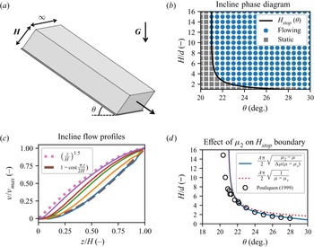
As an initial validation of our numerical approach, we apply it to the case of wide inclined chutes, cf. figure 2(a). This geometry is informative because, as previously described, the NGF model has an analytical solution in this case for the thickness-dependent stoppage threshold, which we can use to validate the code's predictions for non-locally influenced stoppage. Moreover, the NGF model has analytical velocity field solutions in the limiting cases of  $H\sim H_{{stop}}$ and
 $H\gg H_{{stop}}$, which we can also use to check the code. Recall that the present formulation of NGF in our model does not include hysteresis, so
 $H_{{stop}}$ is the same as
 $H_{{start}}$ in what follows; Mowlavi & Kamrin (Reference Mowlavi and Kamrin2021) has explored incorporating hysteresis and non-local effects into a unified model.
Comparing numerical solutions with analytical NGF solutions in the inclined chute. (a) Configuration of the inclined chute geometry. (b) Phase diagram shows the analytically predicted phase boundary (solid black) and MPM simulation results – each blue dot is a simulation that appears to flow, while each grey rectangle is a simulation that appears to stop after initial flow. (c) Flow profiles from MPM simulations are taken at an incline of 27 degrees with layer thickness varying through  $H/H_{{stop}}$ values of 1.9, 2.9, 4.8, 6.8 and 19 (from bottom to top). (d) Analytical solutions for the fit of the
 $H_{{stop}}$ curve showing the difference between using a common limiting stress ratio of
 $\mu _2$ (solid blue) and assuming no limiting value (dotted red). For comparison, experimental data on glass beads are shown (from Pouliquen Reference Pouliquen1999). Material parameters: (b,c) use
 $A = 0.25$,
 $\mu _s = 0.3819$ and
 $\mu _2 = 1.5$,
 $\rho _s = 2450$ kg m
 $^{-3}$,
 $d = 5$ mm and (d) uses inputs for glass beads (from Kamrin & Henann Reference Kamrin and Henann2015)
 $A = 0.48$,
 $\mu _s = 0.3819$ and
 $\mu _2 = 0.6435$.

In our simulations, which are implemented as 2-D plane strain, we use a single column of elements with  $\Delta x = \Delta y = 1\,\textrm {mm}$. We represented the body with a uniformly spaced
 $4\times 4$ arrangement of material points (16 total) per element. Periodic boundary conditions are applied to simulate an infinite chute by using the same node for both the left and right sides, effectively converting this into a 1-D problem along the vertical (although material points are still free to move in both dimensions). Recall that, for
 $g$, the bottom boundary uses a Dirichlet
 $g = 0$ condition while all other sides use a Neumann
 $\partial _n g = 0$ along the normal to the boundary. We take the grains to be glued to the bottom boundary (via a Dirichlet
 $\boldsymbol {u} = 0$ no-slip condition). Common to all included chute simulations, the grain size is given by
 $d = 5$ mm and the solid density of grains is
 $\rho _s = 2450$ kg m
 $^{-3}$. Values for
 $A$,
 $\mu _s$ and
 $\mu _2$ vary as indicated in figure 2. The specific body force is gravity,
 $\boldsymbol {G}$, with
 $|\boldsymbol {G}|=9.81$ m s
 $^{-2}$.
Common to all non-local simulations, we need to provide initial conditions for  $g$, but we require a trick to do this due to a feature of the NGF evolution equation. Note that
 $g = 0$ is always a solution to the PDE, corresponding to a no-flow state, however, it may not always be the stable solution. In reality, infinitesimal fluctuations are ever-present and serve to ‘seed’
 $g$, allowing non-zero
 $g$ solutions to arise. However, we can exactly represent the zero state during computation, and during a normal update there is no automatic numerical seeding process.
In order to allow a flowing solution to develop at all, we instead use the local  $\mu (I)$ model for a short period of time to obtain a flow field, and initialize the value of
 $g$ based on this local flow. This non-zero value of
 $g$ is then evolved to the steady-state solution via the NGF equation. Currently, experimental values of
 $t_0$ are unknown, so for our purposes we choose a small
 $t_0$ in order to reach steady state quickly without adversely affecting the time step size. The results are insensitive to details of this choice –
 $t_0$ can get an order of magnitude smaller or larger without much issue aside from computational time – but for completeness, we used
 $t_0 = 1$ ms with an initialization time of
 $10 t_0$ through all simulations in this work. Simulations were run out to
 $t_f = 20$ s to get a close approximation to the steady-state behaviour, and the time spent in the local state is only a tiny fraction of the total run time.
Each simulation uses a time step size of  $\Delta t = 3\times 10^{-6}$ s and took between 20–30 min of wall time on an Intel Silver 4112. Substepping is not used for the presented results (that is
 $\Delta t_{{substep}} = \Delta t$) as the total wall time was low, however, we checked that setting
 $\Delta t_{{substep}} = \Delta t / 15$ did not change the outputs. Figure 2(b) shows the analytical solution for
 $H_{{stop}}$ from (3.1) together with an array of data points obtained from distinct numerical simulations of our MPM code. Determining if a simulation is truly stopped numerically is difficult, but for our purposes we look simply at the mass-averaged kinetic energy of all the material points in the simulation and compare it with a threshold. We chose
 $1\times 10^{-10}$ J kg
 $^{-1}$, but the results are largely insensitive to the specific value. Similarly, other criteria such as average velocity or total momentum result in identical or nearly identical phase diagrams. It can be clearly seen that our code matches the analytical solution with regard to the placement of the flow/no-flow phase boundary. Also, when a chute does flow, the NGF model has an analytical velocity solution in certain cases, see Kamrin & Henann (Reference Kamrin and Henann2015) for details. For shallow layers near
 $H_{{stop}}$, the last term in the NGF PDE (2.1) is negligible, leaving a linear system whose solution, upon applying the given boundary conditions, is
 $v\propto 1-\cos ({\rm \pi} z/2H)$. On the other hand, for very tall layers, the non-local effect is negligible, and the NGF equations give a velocity field approaching the classical Bagnold solution,
 $v\propto (z/H)^{3/2}$. Figure 2(c) compares these limiting solutions with output solutions of the MPM code for a wide variety of filling heights. It can be seen that the MPM solutions capture these limiting cases and indicate how the solution's concavity changes as
 $H$ increases, a well-known effect observed in experiments (Silbert et al. Reference Silbert, Landry and Grest2003; MiDi Reference MiDi2004).
Regarding flow thresholds, in view of (3.1), we see that NGF predicts  $H_{{stop}}$ vanishes when
 $\tan \theta =\mu _2$; above this tilt angle, the model predicts all chutes flow regardless of filling height (Pouliquen Reference Pouliquen1999). This feature is common among many experimental fits for
 $H_{{stop}}$ (MiDi Reference MiDi2004), and leads correspondingly to fits of
 $\mu (I)$ that also depend on a threshold
 $\mu _2$ (Jop, Forterre & Pouliquen Reference Jop, Forterre and Pouliquen2005). However, there is debate in the experimental literature on the value of
 $\mu _2$, with some even suggesting it may be infinite (Holyoake & McElwaine Reference Holyoake and McElwaine2012). In fact, a linear
 $\mu (I)$ fit function is commonly used in practice for numerical experiments (da Cruz et al. Reference da Cruz, Emam, Prochnow, Roux and Chevoir2005) and in coarse-graining analysis (Weinhart et al. Reference Weinhart, Labra, Luding and Ooi2016), which amounts to setting
 $\mu _2=\infty$. If one tries to infer
 $\mu _2$ from
 $H_{{stop}}$ data by observing the tilt at which all chutes flow, complications may arise since this point is not always easy to identify, as it requires measuring
 $H_{{stop}}$ when its value is
 ${\lesssim }1d$. In fact, even if one chooses
 $\mu _2=\infty$ in the NGF solution form, the
 $H_{{stop}}$ curve changes only very little. For example, in figure 2(d) it can be seen that the stopping curves under NGF for a common value of
 $\mu _2$ and for
 $\mu _2=\infty$ differ only at the tail and both seem adequate to fit experimental data. The ambiguity in the choice of
 $\mu _2$ with respect to inclined flow arrest will come to use in the upcoming section on silo clogging, where certain constraints on the size of
 $\mu _2$ exist a priori.
7. Silos
We now turn our attention to the silo geometry. As we have verified the non-local effects are properly captured in the simpler inclined chute flow, through this section we now show that the same continuum model and method can be used to determine if a silo should clog or flow based on the material and geometric properties as inputs. We first use several simulations and populate a phase diagram to get an idea of the stability of the clogged solution as a function of  $A$ and
 $W/d$. As further outputs, we will show the arch shape (when clogged), as well as pressure, velocity and
 $g$ fields (in both clogged and flowing cases). In flowing cases, we also look at horizontal slices of vertical velocity profiles, and note the spreading Gaussian form as has been reported previously. Finally, we conduct a short convergence test to show that refinement in space and time produces qualitatively similar results – clogged silos remain clogged, although with a more refined arch, and flowing silos maintain a similar flow rate and pressure distribution.
7.1. Silo geometry and numerical parameters
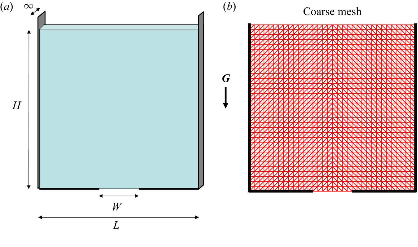
Our implementation is in 2-D plane strain, corresponding to a thick silo in the out-of-plane direction. When choosing the geometry of the mesh, note that the silo needs to have enough elements across the orifice to initiate and resolve the flow (in a flowing case), but to reduce computation time we would like to keep this number manageable. We chose 8 units across the orifice, with each unit being a 0.0175 by 0.0175 m square. Although the background mesh is ephemeral in MPM, since we solve the equations of motion over this mesh it does have an influence on the space of possible solutions on the material points. As with the inclined chutes, each square unit contained 16 material points (four per spatial dimension). In order to reasonably match the geometry of an arch, each unit consists of two triangular elements with the diagonal going from bottom left to top right for the left half of the silo and vice versa for the right half (see figure 3b). We show later that results are insensitive to the exact number of elements as long as there are enough to resolve flow features around the orifice. A full convergence study is not attempted in the present work, as the computational time and space required quickly becomes prohibitive due to the explicit parts of the scheme and the number of auxiliary variables respectively.
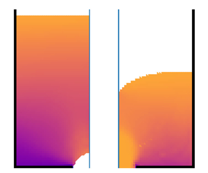
The geometry of the silo is shown in (a). We kept the height  $H$, width
 $L$ and orifice width
 $W$ consistent throughout the simulations and changed the material parameters, mainly grain size
 $d$ and non-local amplitude
 $A$. The background mesh used by the MPM scheme for coarse cases is shown in (b) to aid in understanding the apparent shape of the arch in static cases.

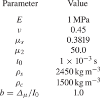
Material parameters are presented in table 1, which are largely consistent with values commonly used for a 3-D packing of glass beads. Of note, however, is the large value of  $\mu _2$, explained as follows. At a jammed arch in a plane-strain silo, the stress state must be compressive along the arch, but vanish normal to it because it is a free surface. Thus, the stress state at the arch must attain
 $\mu = 1$; this fact is true regardless of the constitutive model, and we have observed this in our own results. Note that this does not apply to flowing silos. In the flowing case, a local
 $\mu (I)$ model would give that if any shear is present on the boundary between dense and disconnected states then
 $\mu = \mu _2$, and our simulation outputs do indicate
 $\mu \approx \mu _2$, although we are unsure if a non-local model must also attain exactly
 $\mu _2$ or simply a value greater than one. To properly capture the clogged stress state, it follows that
 $\mu _2$, the feasible upper limit for
 $\mu$ in models like ours that extend the
 $\mu (I)$ rheology, cannot be less than
 $1$. The constraint is slightly weaker for fully 3-D silos with a hole orifice, where
 $\mu _2$ must exceed
 $\sqrt {3}/2\approx 0.866$ to admit a jammed arch state (and an overall clogged silo). Both these values are higher than, for example,
 $\mu _2=0.6453$ reported in Jop et al. (Reference Jop, Forterre and Pouliquen2005), but recall from the section on inclined chutes that there is ambiguity on the value of the upper limit of
 $\mu$ and little experimental data in that regime. We observed in our simulations that above
 $\mu _2\sim 10$, the solution becomes insensitive to the value of
 $\mu _2$ so we simply set
 $\mu _2$ to an asymptotically high limit, giving effectively a linear
 $\mu (I)$ fit in the local limit.
Common material parameters used for the silo simulations. Our simulations vary  $A$, hence it is not present in this table, but instead will be specified on a case-by-case basis.

Each simulation is run with the same orifice size  $W$, given by 0.014 m (measured from fixed node to fixed node), but the grain diameter
 $d$ is varied via the material properties to set the ratio
 $W / d$. The total width of the silo
 $L$ is fixed at 0.595 m (34 units) and, importantly, the same background mesh and material point density is used for all simulations so as to control the possible influence of numerical length scales. The initial fill height
 $H$ is also fixed at 0.595 m. Initially, the material point configuration is assigned a lithostatic pressure; the density of each material point is set to be commiserate with this pressure by computing
 $\rho = \rho _c K / (K - p)$, where
 $K$ is the bulk modulus and
 $p$ is the pressure of that material point. The density is initially set by changing the mass of the material point – all material points have the same initial volume in these simulations. However, as in Dunatunga & Kamrin (Reference Dunatunga and Kamrin2015), the true volume of material points evolves over time (although the numerical extent they are integrated over does not, see Appendix B).
Similar to the inclined chutes, we set the bottom of the silo to have Dirichlet  $g = 0$ and
 $\boldsymbol {u} = \boldsymbol {0}$ (no-slip) boundary conditions – note these are only applied along the solid portion of the boundary (i.e. they do not apply directly over the orifice, which instead allows the granular material to act as a free surface with
 $\partial _n g = 0$ and a traction-free condition). The sidewalls allow friction-free sliding (perfect slip), but do not allow material points to go through the boundary; that is
 $v_n = 0$ while the transverse direction is unhindered, and
 $\partial _n g = 0$.
No motion is imparted to the material points as an initial condition. Instead, the retaining wall at the orifice is removed upon the first step of the simulation and flow is allowed to develop ‘naturally’. Recall from the section on inclined chutes that we initialize  $g$ by running the local model for a short period of time. As the local model will always produce a flow field regardless of the ratio of orifice to grain size, this procedure will always result in a non-zero
 $g$ field. After initializing with the local model, the numerical procedure detailed above for the non-local model is used to determine if the solution decays towards a stable
 $g = 0$ state corresponding to a clogged silo or evolves to obtain some other steady flowing state.
We found the results largely insensitive to the specifics of how the seeding procedure was performed; changing from a local model  $\mu (I)$ to a simple rate-independent Drucker–Prager material only slightly affected transient states after switching to the non-local procedure, and decreasing or increasing the local model run time similarly had almost no discernible effect on the final state. There were two notable exceptions to this. First, if the material points deviate too much from their initial positions, finding a non-flowing solution became difficult, at least at the spatial and temporal sampling parameters we had used. This is likely because a strong arch of material points needs to develop simultaneously without any holes, and as points move further from their initially ideal placement, numerical noise in MPM makes this unlikely. Refinement would likely mitigate this issue, as the crossing noise can be reduced and the additional material points are more likely to sample a good configuration for numerical purposes, but we did not explore this further. Secondly, if the initialization process were done too quickly, the flow field (and therefore
 $g$) may not have enough time to establish through the system and ends up too small in magnitude to seed the simulation in light of numerical damping.
Outside of initialization, elastic waves through the system may serve to jostle a clogged silo away from that state. These elastic waves may cause fluctuations in  $\mu$, which can interfere with the evolution of
 $g$. While some of these effects are physical, real systems also include elastic-wave damping effects not included in our model; moreover, we are most interested in the elastically rigid limit where elastic waves would not occur anyway (the motion would simply be unsupported by the system). With a high (but finite) wave speed, the time scale for inertial variation is far larger than that of elastic waves, so even a small amount of dissipation should cause elastic waves to dissipate quickly relative to the amount of time it takes for macroscopic granular flow features to appear or change. Adding bulk viscosity could be one approach to adding a controlled dissipative term, but after observing preliminary results with this enabled, we felt it interfered too much with the solution. Instead, we implemented an elastic-wave absorbing boundary by zeroing out the speed of any material point moving upward that is located at
 $y$-position 0.49 m (28 units) or higher. Upward motion is entirely caused by elastic waves in this problem since gravity points down. This absorbing condition is located sufficiently far from the orifice that we believe it should not affect any true dynamics near the opening when the system clogs or in flowing cases while serving to remove unwanted elastic waves. Results were largely insensitive to the position or strength of the penalty (e.g. moving the dividing line down by 8 cm did not change the results of our analysis, nor did implementing the penalty as a halving of upward velocity instead of zeroing).
7.2. Silo clogging phase diagram
Even if it may be obvious to the eye, determining a precise criterion for when a silo configuration is clogged in a numerical simulation is a non-trivial exercise. It can be comparable to studying avalanche effects and the presence of open/falling material can trick kinetic-energy-based criteria for solidification (Aranson & Tsimring Reference Aranson and Tsimring2001; Martin et al. Reference Martin, Dubois, Monerie and Radjai2009). Instead, we use a heuristic to mark states as ‘likely static’, ‘likely flowing’ and ‘unsure’. If the average velocity of the dense material is small and at most exhibits decaying oscillatory waves, we suspect that the material is in a static configuration. Additionally, if the mass flow rate out of the orifice corresponds to only a few grains per second, we can be more sure that the configuration is static. Conversely, if the average velocity points downward, is large, and does not change size much, we suspect that the material is flowing; we can be even more sure if a large number of grains are leaving per unit time. To make this more precise, in our simulations we check if the most recent zero crossing of the vertical component of velocity happened within the last ten per cent of the simulation; if so, we give a point in favour of a static configuration. If the last zero crossing happened earlier than half-way through the simulation, we give a point to the flowing state; in between, we are unsure. We then check the number of material points leaving between each saved frame of the simulation; if this is less than or equal to one on average in the last tenth of the simulation (with our parameters, this is a mass flow rate of 28.7 g s $^{-1}$ per unit width), that is a point in favour of a static configuration. If this is greater than ten per frame on average, that is a point in favour of a flowing simulation; in between, we are unsure. Both tests must agree (i.e. two points are required for us to mark the simulation as static or flowing) – any other state is marked as unsure. Visual inspection of the last few frames of a selection of simulations was also done for confirmation.
Simulations took approximately 2 hours on an Intel Silver 4112, with faster-flowing simulations finishing earlier as they had fewer material points over time. In all silo simulations, we used a substepping time of  $\Delta t_{{substep}} = \Delta t / 150$, which we estimate from smaller cases reduced the wall time by a factor of two. Using the criteria outlined above, we plotted these data on a lattice with simulations having varying
 $A$ and
 $W/d$ ratios (as
 $W$ is fixed, we simply changed the material grain size
 $d$ to achieve the desired ratios). The value of
 $A$ is either
 $0.1$,
 $0.5$,
 $1.0$,
 $1.5$,
 $2.0$,
 $2.5$ or
 $3.0$ while
 $W/d$ must be either
 $1$,
 $2$,
 $3$,
 $4$ or
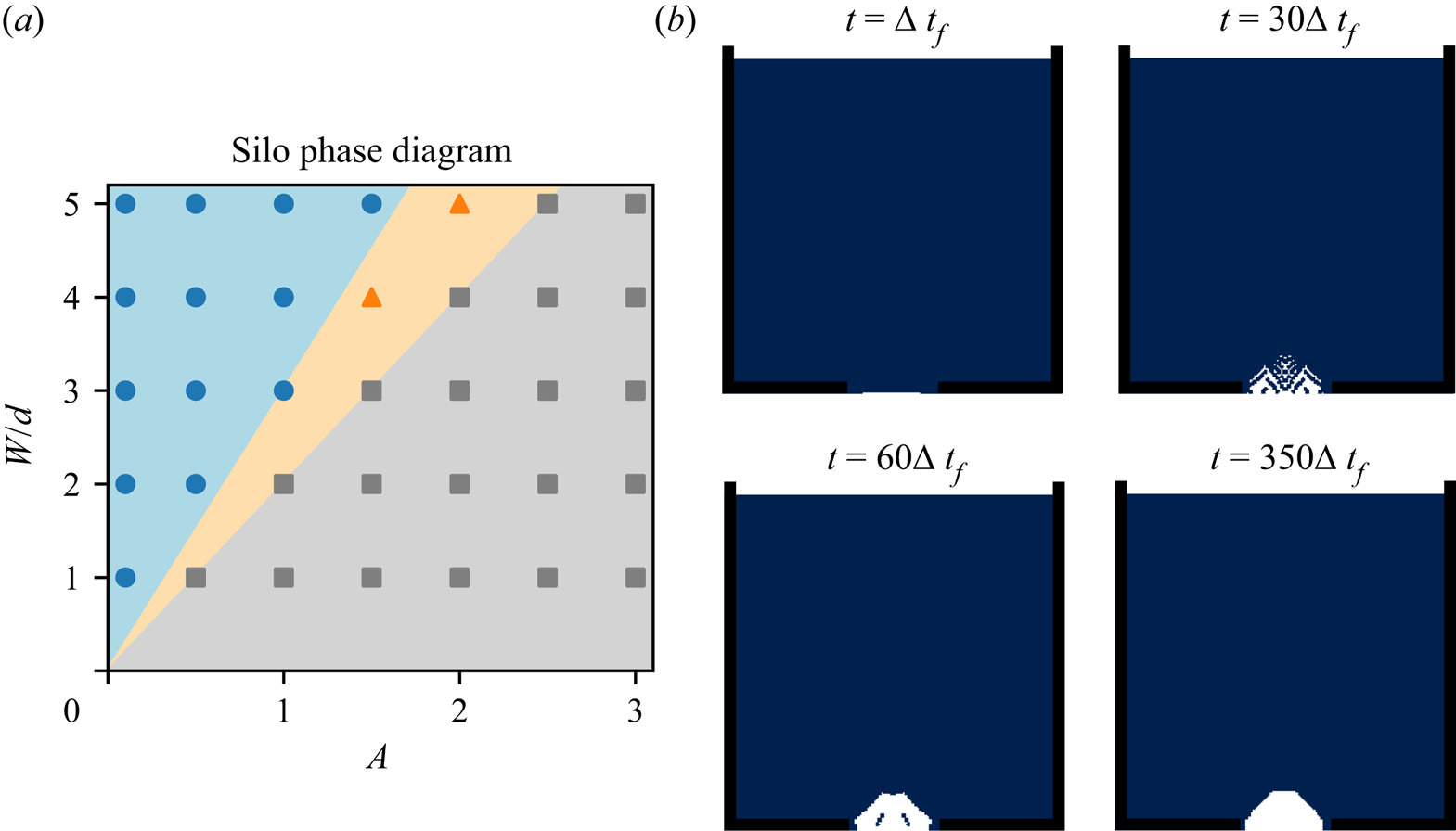
 $5$. The results are shown in figure 4(a). Note that we see a separation into three regions (flowing, static and unsure) which can be well described simply by two lines of different slope; the ratio of
 $W/d$ to
 $A$ seems sufficient to predict if a simulation will flow or reach a static state.
(a) Silo phase diagram varying non-local amplitude  $A$ and the relative opening size
 $W/d$. A blue circle means the simulation flows, a grey square means the simulation attains a static configuration and an orange triangle indicates that we were unsure how to classify the simulation – see the main text for details on the classification criteria. Note that the geometric properties of the simulation were held constant and that only the indicated material properties of the NGF model (that is, the grain size
 $d$ and
 $A$) were varied here. All other material properties were held constant for these tests. Note that the diagram can be partitioned into the three regions with only two lines which go through the origin. (b) Still frames of the arch formation process for the
 $A = 1.0$,
 $W/d = 1.0$ case, which is a static simulation in our classification.

This is not too surprising if we consider the form of the NGF PDE and the set-up we used. Note that the term  $d$ almost always appears with
 $A$ – it only shows up alone in the
 $g^{2}$ term for describing the local rheology, which we believe only has a minor effect on the stability of the solution. Since
 $W$ is fixed in these simulations, lines of constant
 $Ad$ should therefore exhibit very nearly the same stability behaviour, as the only difference would appear in the
 $g^{2}$ term. In our graph, starting at the origin, we can fan out to form these lines of constant
 $Ad$, and we do see a physically reasonable boundary between flowing and non-flowing cases. Keep in mind that the ‘unsure’ cases and region correspond to error bars in our classification – we believe the ‘true’ boundary is indeed nearly a straight line within this uncertainty cone relating
 $Ad$ to
 $W$. As a benchmark against experimental data, note that at
 $A = 0.5$ (an approximate value for 3-D beads) the flowing/static boundary occurs somewhere between
 $W/d = 1$ and
 $W/d = 1.5$. This corresponds well with experimentally observed values for the critical
 $W/d$. In the flat-bottomed quasi-2-D silo, which we are attempting to model,
 $W/d\approx 1.0$ was obtained for beads in Choi et al. (Reference Choi, Kudrolli and Bazant2005). This is similar to the range of 1.0–1.16 that was obtained in Mankoc et al. (Reference Mankoc, Janda, Arevalo, Pastor, Zuriguel, Garcimartín and Maza2007) for beads, albeit for a circular orifice. As before, we note that since we have a continuum solver, we achieve the static configuration when the ensemble average behaviour would be to form a static arch. In a single experiment, it may be possible to observe orifice openings of larger size that nevertheless still can find a static configuration, but these become rare as the ratio
 $W/d$ increases. Figure 4(b) shows an example of an arch forming in one of our continuum simulations (where
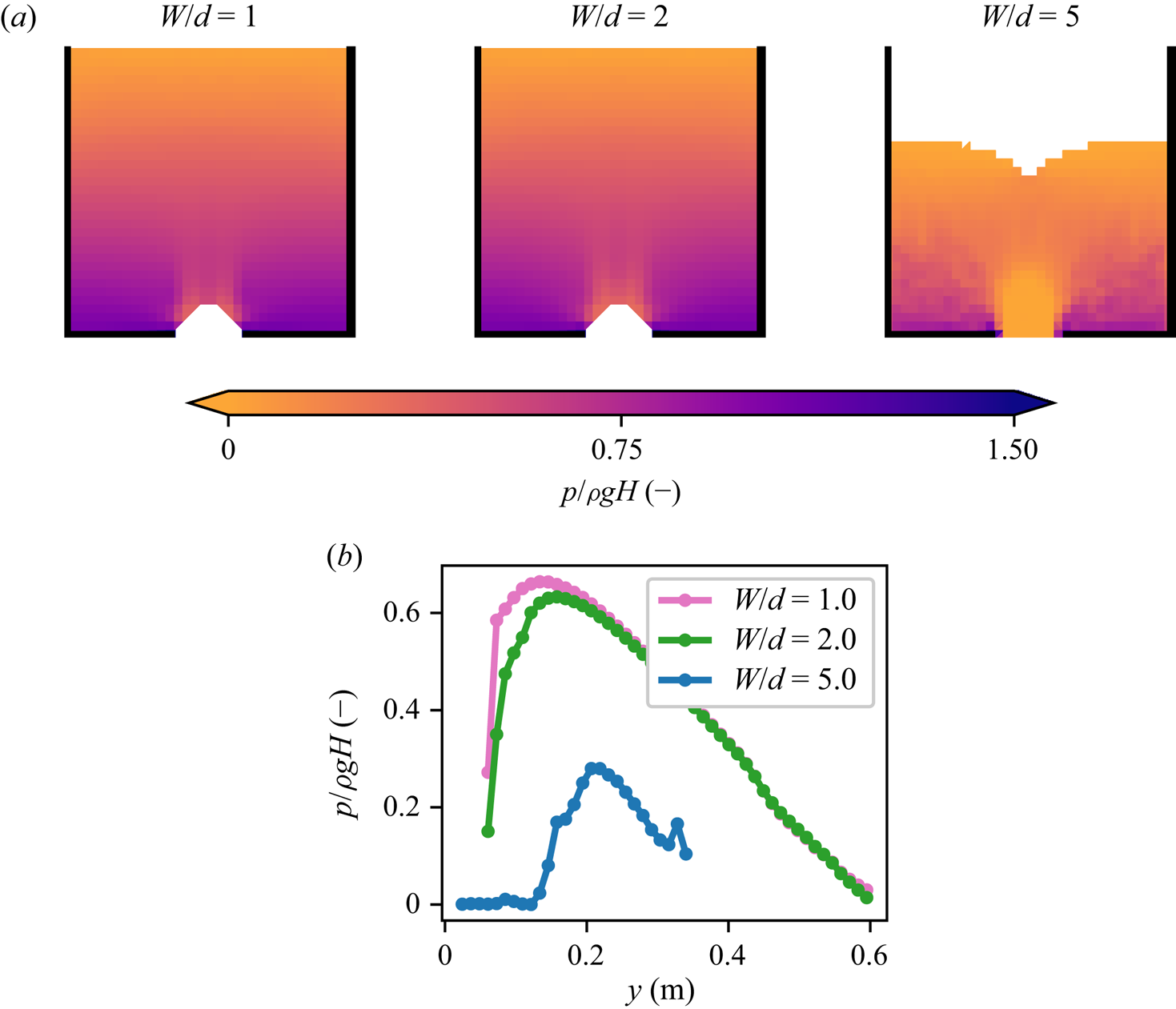
 $\Delta t_f = 1/240$ s) when the silo opening is sub-critical, with material points below the arch falling out leaving the rest of the silo material intact as the fluidity decays to zero. The numerical procedure models the outline of the material domain from edges of the background mesh geometry, which leads to a ‘polygonal’ arch shape; as the mesh refines more, a rounder arch shape emerges (see § 7.3 and Supplemental Movie available at https://doi.org/10.1017/jfm.2022.241). Next, in figure 5(a), we observe the pressure distributions in the silos for three configurations
 $W/d = 1$,
 $2$ and
 $5$ with a common
 $A = 1$. The fields are plotted near the end of the simulation and use a spatial and temporal average over frames from
 $350 \Delta t_f$ to
 $360 \Delta t_f$. The spatial smoothing was done as in Andersen & Andersen (Reference Andersen and Andersen2009) to project point-wise pressure data onto the background mesh – note that this is a purely visual post-processing technique and does not affect the fidelity of the simulation itself. In the clogged configurations (
 $W/d = 1$ and
 $2$), we see that the pressure immediately above the arch is low, but does not go to zero. The simulation which is closer to the static/flowing boundary (
 $W/d=2$) experiences a lower pressure in the region immediately above the arch, although some distance away from the opening the pressure looks essentially the same as the other static case. In contrast, the flowing simulation (
 $W/d = 5$) contains many materials points in the region above the orifice where material points are in free fall, and the pressure indeed goes to zero when approaching this region since the material points are stress free. The peak pressure is also smaller, although the fill height has already decreased substantially by the time this snapshot was taken due to the flow. Figure 5(b) uses the same data, but shows the pressure along the vertical centreline of the silos, confirming our observations from the patch plots.
(a) Visualization of pressure in silos with  $A = 1$ and
 $W/d = 1, 2$ and
 $5$ (left, centre and right, respectively). These correspond to data points in the
 $A=1$ column of figure 4(a). The pressure shown here is a temporal average projected onto the mesh over several neighbouring frames from the view of grid elements (from
 $350 \Delta t_f$ to
 $360 \Delta t_f$ inclusive). White corresponds to a completely empty element. (b) Plots of the pressure along the centreline for silos with
 $A=1.0$ and
 $W/d$ ratios of 1.0, 2.0 and 5.0 (pink, green and blue, respectively). While the pressure decreases drastically directly above the orifice in the clogged configurations, it does not reach zero. In contrast, the flowing case has much lower pressure and is actually zero in the region above the opening.

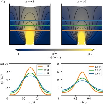
Now we will turn our attention more towards the flowing simulations. In figure 6 we compare two silo flows which have the same material parameters but different values of  $A$. Snapshots are taken at slightly different times to account for the difference in outflow rates and were chosen to keep a similar amount of mass remaining in the silo; the snapshot for the
 $A = 0.1$ case is taken at
 $70 \Delta t_f$ and for the
 $A = 1.0$ case is taken at
 $86 \Delta t_f$, where again
 $\Delta t_f = 1/240$ s. In the top half of figure 6, we see the velocity fields plotted over material points and velocity contours. The spacing of the contour lines indicates that shear zones in the
 $A = 0.1$ case (left) are thinner than in the
 $A = 1.0$ case (right). This is confirmed by plotting the vertical velocity across horizontal slices at heights
 $1.5W$,
 $2.0W$ and
 $2.5W$ in the lower half of the figure – the flow is more plug like in the low
 $A$ case, and is noticeably similar to a local
 $\mu (I)$ model solution, which would predict plug flow down the centre with a thin shear band before dropping to zero vertical velocity close to the sidewalls where
 $\mu < \mu _s$ (Kamrin Reference Kamrin2010; Staron et al. Reference Staron, Lagrée and Popinet2012; Staron, Lagrée & Popinet Reference Staron, Lagrée and Popinet2014). In contrast, the higher
 $A$ value results in a spreading of the velocity field as expected due to the non-local effect, which will imply a length scale for shear bands. As both cases do actually have non-zero
 $A$, we do observe a small amount of flow even where
 $\mu < \mu _s$ as expected, and less flow under
 $\mu _s$ is observed for the smaller
 $A$. The decay length scale depends on the size of
 $A$, and we find that larger
 $A$ diffuses out the velocity more readily, also as expected.
Two silos with the same parameters and initial conditions except for the value of  $A$. Both simulations have nearly the same amount of mass remaining in the silo when imaged (
 $70 \Delta t_f$ left,
 $86 \Delta t_f$ right). The velocity cuts off more sharply in the low
 $A$-value case as expected. Iso-speed lines (drawn at 0.05, 0.10, 0.15, 0.20, 0.25, 0.30 and 0.35 m s
 $^{-1}$) are drawn over a scatterplot of the speed confirm that the velocity is diffusing more when
 $A=1.0$ compared with when
 $A=0.1$. Vertical velocity profiles are drawn at the heights indicated as horizontal lines in the first row of images located at heights
 $1.5W, 2.0W$ and
 $2.5W$ above the orifice. The grain size is given by
 $d = 0.028$ m, and the orifice size is
 $W = 0.14$ m resulting in
 $W/d = 5$.

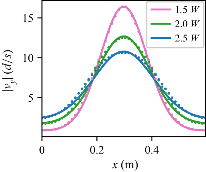
We also look at the form of the vertical velocity profiles obtained. In order to compare with existing data, which uses glass beads primarily, we choose  $A = 0.5$ and set
 $W/d = 5$. We waited for steady-state flow, and then looked at vertical velocity slices at the same three heights as before (
 $1.5W$,
 $2.0W$ and
 $2.5W$); results are plotted in figure 7. Many have noticed in experiments that the downward velocity profile, in a region not too far from the opening, appears to spread diffusively but with height playing the role of ‘time’ — that is, the downward velocity appears Gaussian with
 $v_y=C \exp {{-x^{2}}/{4By}}$ where
 $B$ controls the width of the Gaussian and
 $y$ is the height above the orifice (Tüzün & Nedderman Reference Tüzün and Nedderman1979; Medina et al. Reference Medina, Cordova, Luna and Trevino1998; Samadani, Pradhan & Kudrolli Reference Samadani, Pradhan and Kudrolli1999; Choi et al. Reference Choi, Kudrolli and Bazant2005; Bazant Reference Bazant2006; Rycroft et al. Reference Rycroft, Bazant, Grest and Landry2006; Zuriguel et al. Reference Zuriguel, Maza, Janda, Hidalgo and Garcimartín2019). The apparently diffusive character of the flow field was central to some of first silo flow models (Mullins Reference Mullins1972; Nedderman & Tüzün Reference Nedderman and Tüzün1979). Interestingly, data from our simulations also match this observation, see figure 7, with two caveats. First, we have an additive constant at each height due to our walls having no friction (and thus allowing downward motion at the walls); in experiments, wall friction ensures velocity decays to zero at the sidewalls. Secondly, the width parameter that we obtain,
 $B = 0.6d$, is a smaller than the typical values observed in the literature (
 $1d$–
 $5d$ in Kamrin & Bazant Reference Kamrin and Bazant2007). We believe this is due to the relatively large orifice size we used compared with the geometry of our system (unlike the experiments which used a much smaller opening relative to the silo width) as well as the aforementioned lack of sidewall friction. Recent studies (Pongó et al. Reference Pongó, Stiga, Török, Lévay, Szabó, Stannarius, Hidalgo and Börzsönyi2021) have shown the flow rates are also a function of particle stiffness. Possibly related effects such as layering near boundaries are not presently incorporated in the continuum model, so exploration of boundary conditions and edge effects are natural areas for future work. Finally, we plot the
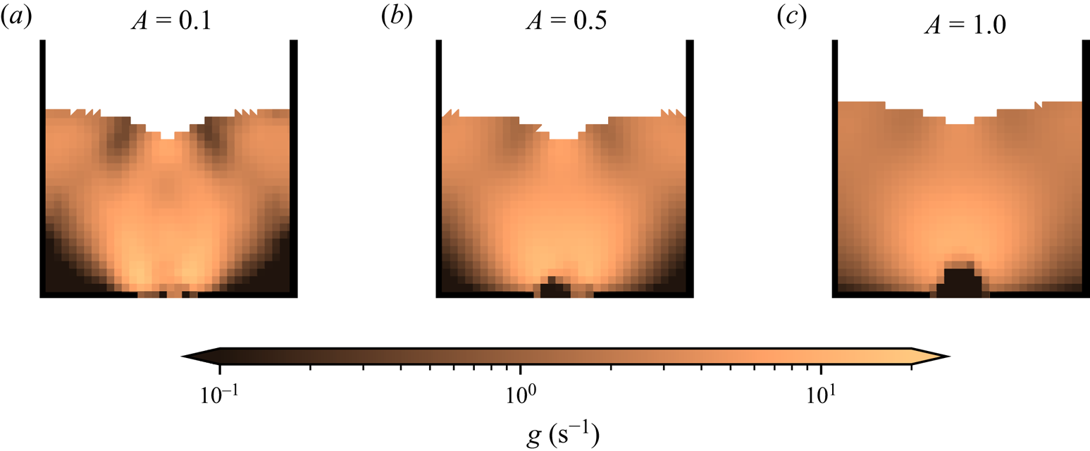
 $g$ field in these same simulations, shown in figure 8 (note that these cases correspond to the top left of figure 4(a) – all of them flow, even
 $A = 1.0$). The plots show averages over both elements and temporal frames (
 $280 \Delta t_f$ to
 $300 \Delta t_f$) to understand what the numerical scheme regularly observes when computing the spatial gradients. Note that the lower values of
 $A$ show less spreading of the
 $g$ field and a slightly larger flow rate compared with higher values of
 $A$ (indicated by the height of the free surface) as expected. Considering
 $g$ as a surrogate for equivalent plastic shear strain rate, we can also observe the distinctive ‘arms’ of high shearing emanating from the orifice. The region just above the orifice where grains are in free fall is also clearly visible in these plots, indicated by a dark brown colour (
 $g$ is set to zero in the disconnected state, but those material points do not contribute to the solution of the NGF equation).
Cross-sections of vertical velocity taken at horizontal slices at height  $1.5W$,
 $2.0W$ and
 $2.5W$ (pink, green and blue colours, respectively) in a silo with the same parameters as figure 6 except
 $A = 0.5$ (chosen to match experimental material). Simulation data are plotted with dots, while a diffusing Gaussian fit (with offsets) is plotted as the lines. The value of
 $B$, which controls the Gaussian's width at each height, is given by
 $0.6d$ (
 $d$ grain diameter).

Plots of  $g$ (logarithmic scale) of a silo with
 $W/d = 5$ and the same material parameters as previously used except in the value of
 $A$, going from
 $0.1$ to
 $0.5$ to
 $1.0$ from left to right. Our averaging procedure assigns the value of
 $g = 0$ to open material; the region immediately above the orifice appears to have low
 $g$ value, although it may be more correct to say there is no value of
 $g$ at those points, as they are stress free in the disconnected state in our model. All plots are taken over an average of frames from
 $280 \Delta t_f$ to
 $300 \Delta t_f$ and use the same mesh-wise projection technique as was used to display the pressure in figure 5. Note that the lower values of
 $A$ result in less spreading of the
 $g$ field, as anticipated.

7.3. Convergence test and caveats
Convergence testing is difficult due to the amount of wall time each simulation takes and the total amount of data generated. Performing a (linearized) von Neumann stability analysis on the scheme used for evolving the NGF PDE shows that the stable  $\Delta t$ is proportional to
 $\Delta x^{2}$ due to the Laplacian term (Dunatunga Reference Dunatunga2017). While the substepping is designed to mitigate the impact of this harsh Courant–Friedrichs–Lewy (CFL) condition, running a refined simulation still takes substantially more CPU and wall time than a coarse one.
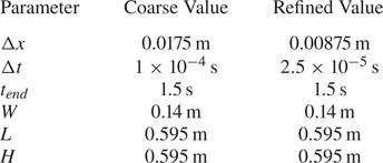
To at least show qualitative agreement, we performed another set of simulations at twice the spatial resolution of the previous cases (and correspondingly a time step of one quarter the original size). As with the other simulations, the mesh consists of triangles stacked to create squares, and which diagonal used depends on which half of the domain the element is in. Numerical parameters are summarized in table 2. We choose  $A = 1$ and other material parameters are given as before in table 1. In summary, we consider a total of four simulations in this section; we look at all combinations of two different refinement levels and two different grain diameters. We wish to observe agreement in the silo geometry as well as fields such as the velocity and pressure.
Numerical parameters used for the refined and coarse simulation cases used in the convergence study. The only differences are that the element size is halved and the refined time step size is correspondingly cut down to a quarter of the coarse value. The material properties are given in table 1.

Our coarse simulations use the same data as before, with a grid size of  $\Delta x = 0.0175\,\textrm {m}$, a time step size of
 $\Delta t = 1\times 10^{-4}$ s and take around 2 hours to complete on an Intel Silver 4112. In contrast, the refined simulations use a grid size of
 $\Delta x = 0.00875$ m, a time step size of
 $\Delta t = 2.5\times 10^{-5}$ s and take approximately 30 hours to complete on the same machine; both refined simulations were run at the same time, with the only difference between them being the grain diameter
 $d = 0.014$ and
 $d = 0.0028$ m (resulting in
 $W/d = 1$ and 5). See Supplemental Movie for side-by-side video of these simulations. The flowing simulation (with a smaller grain diameter) finishes slightly earlier, as removed material points do not require much computational work to handle. As with the coarse silos, we use substepping with
 $\Delta t_{{substep}} = \Delta t / 150$.
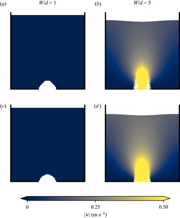
We compared the velocity profile in this refined case with the coarse cases run previously with the results displayed in figure 9. Both the static configuration at  $W/d = 1$ (snapshots taken at
 $350 \Delta t_f$, where
 $\Delta t_f = 1/240$ s as before) and the flowing configuration at
 $W/d = 5$ (snapshots taken at
 $105 \Delta t_f$) show good agreement when refined. The increased resolution allows the arch to form with a slightly more natural circular geometry in the static case. In the flowing case, the refined simulation has a slightly higher velocity throughout the bulk, however, this is expected and is also due to geometric refinement; as we measure the orifice size between the fixed points, decreasing the element size allows a larger fraction of material to leave without sensing the orifice edge. This is a minor effect, but does serve to increase the flow rate a little as observed. We expect subsequent refinements to show increasingly smaller differences in velocity fields since the affected elements will get smaller.
Speed contours of coarse simulations (a,b) and refined simulations (c,d). The  $W/d = 1$ cases are taken at time
 $350 \Delta t_f$ and the
 $W/d = 5$ cases at
 $105 \Delta t_f$ (recall
 $\Delta t_f = 1/240\,\textrm {s}$). The refinement allows a more accurate representation of the orifice size across all simulations and the arch formed in the
 $W/d = 1$ case. Velocities are plotted as given on each material point.

Similarly, we compared the pressure throughout both sets of silos in figure 10. As before, good agreement is shown between the refined and coarse cases. The static case shows a few differences due to the more circular geometry of the arch, however, the key features of small-but-non-zero pressure above the arch and a largely lithostatic pressure distribution away from the orifice remain. In the flowing case, the refined simulation has a noticeably smoother pressure field and resolves the free surface with more fidelity as expected, but otherwise qualitatively looks similar to the coarse case. We can clearly see the free-fall region above the orifice in both cases, where the pressure of the material points goes to zero as they enter the disconnected state.
Pressure distributions of coarse simulations (a,b) and refined simulations (c,d). All plots are taken over a three-frame average centred at  $350 \Delta t_f$. As with the previous pressure plots, the technique presented in Andersen & Andersen (Reference Andersen and Andersen2009) for visualization is used.

To understand the shape of the arch, we turn our attention to the  $g$ field, as
 $g$ controls how much plastic flow occurs in the dense phase. Since entire elements contribute to the
 $g$ field and are not considered at a sub-grid scale, this in turn restricts the shapes that the boundary can take; the effect is most apparent in simulations such as a clogged silo since the arch formed must conform to the background mesh geometry. Sufficient mismatch between the true solution and the one forced by the grid geometry might result in flow where none was expected or vice versa. We only observed this in boundary cases (e.g. in the silo, ones in which we were unsure were flowing or static), but the underlying mechanism may persist in pathological grid topologies. We also note that computing the solution is noticeably more expensive in time than a local version of the model – the extra operations performed do contribute to this, but the increase in number of synchronization points also should not be underestimated. Naively coding the algorithm presented can easily result in a method which is tens to hundreds of times slower than the local-only
 $\mu (I)$ model; while none of our implementations have been heavily optimized, many of the simulations in this work took approximately two to five times longer than our implementation in Dunatunga & Kamrin (Reference Dunatunga and Kamrin2015) of a local-only model implementing the
 $\mu (I)$ rheology from Jop et al. (Reference Jop, Forterre and Pouliquen2006) (caching the results where possible during substepping results in significant time savings). It may be possible to mitigate much of the computational expense by switching to an implicit solver, but this must be done carefully due to the nature of the material tangents. We would like to explore these solvers in future work as they would improve the applicability of the method to engineering problems.
8. Conclusion
We have presented and numerically implemented a trans-phase (disconnection-permitting) extension of the NGF model. Using our implementation, we have shown that NGF, a continuum model, is able to predict the clogging of a silo due to small opening size. This result is analogous to the same model's previously shown capability to capture the strengthening of layers on inclines as they get thinner. We find that when the model's parameters are set close to the known values for spherical beads, the critical opening size obtained is close to the reported experimentally observed range and corresponds to the Beverloo cutoff size. We have also verified by constructing a phase diagram that the criterion for silo clogging in NGF takes the form  $W_{{crit}}\propto A d$ showing the dependence on the model's non-local amplitude,
 $A$, to be a straightforward linear prefactor, and the relevant length scale being the mean grain size, as expected. By including a separated phase within the rheology, the model is able to capture the process of a stable arch forming when a silo clogs, with material under the arch falling out freely. When the opening is large enough to admit a steady flow, we find the value of
 $A$ for a given
 $d$ influences how much the flow spreads spatially, with low values of
 $A$ emulating the purely local response with sharp flow peak in the silo centre that rapidly decays toward the walls, and larger
 $A$ values causing a shallower peak and smoother tapering off toward the walls. Lower
 $A$ values correlate with higher overall outflow rates, which is to be expected since non-locality acts as a flow penalty for sharply varying fields. When the parameters are set to those of spherical beads, we find, similar to previous observations for glass beads in slab silos, that the downward velocity profile along horizontal cross-sections looks similar to a Gaussian spreading diffusively in height.
The versatility of our numerical approach, combining MPM with a simple finite-difference grid, allowed us to numerically solve the NGF model in multiple of inhomogeneous flow geometries. As a validation check, the method reproduced the analytically known velocity profiles and  $H_{{stop}}(\theta )$ curves in the case of the inclined chute. Throughout our study, when comparing silos of different
 $W/d$, we were careful to use the same grid and initial material point distribution so as to ensure the numerical scheme does not bias the critical opening size in any suite of tests. Finally, we showed that refining the silo geometry discretization results in qualitatively very similar behaviour with only minor differences due to increased spatial resolution.
This study leaves at least two interesting theoretical questions. The first is in reference to the value of  $\mu _2$ and whether this parameter, which carries over from the local
 $\mu (I)$ model, should in fact be bounded. Secondly, the value of the fluidity-diffusion time scale
 $t_0$ has not been previously quantified in experiments, hence our study has chosen it to be sufficiently small compared with all other time scales so as to deliver
 $g$ distributions that are stable and quasi-steady. More study would be needed to correctly characterize this material parameter for more transient applications.
Supplementary movie
Supplementary movie is available at https://doi.org/10.1017/jfm.2022.241.
Declaration of interests
The authors report no conflict of interest.
Appendix A. Discussion of alternative methods
The numerical solution of the continuum equations of motion is typically done via one of two broad classes of methods; those which track a section of the body over time, obtaining a history of positions and velocities (Lagrangian methods), and those which track a volume of space over time, obtaining a history of the material which entered and exited the domain (Eulerian methods).
Of the Lagrangian methods, the FEM is widely used for solid mechanics. FEM divides up a body into smaller elements, each of which can be described with a small set of state information. FEM typically takes displacements on nodes of these elements as the degrees of freedom, so each element tracks the same part of the body throughout the entire simulation. This is usually achieved by using the Galerkin Method to obtain a system of equations where the coefficients are sums of integrals over elements (and then solving the system via numerical linear algebraic methods). However, this places restrictions on the types of deformations allowed. Specifically, large nonlinear deformations are problematic, as they usually distort the mesh such that quadrature over an element does not yield accurate results.
In contrast, finite volume methods are common in fluid simulations. These are Eulerian methods in nature, performing all operations of a fixed grid. Material may move in and out of cell boundaries, or even leave the domain of interest entirely – the elements are fixed in space and not tied to a particular parcel of fluid. These methods have a complimentary set of strengths and weaknesses as compared with FEM; they can handle large inelastic deformations easily, but have difficulties representing material boundaries and material state fields, including strain, as needed for static elastic solutions.
In most cases, the limitations of each method are less problematic than they might first appear; simulation of solid material typically will not involve the large nonlinear deformations that are fatal to regular FEM, and rarely does a fluid simulation require accurate representation of a static elastic configuration. But granular materials are an interesting exception, as they show a rich variety of behaviours. Even within the same simulation, a granular material may flow like a fluid, disperse into a gas-like state, and finally form a static configuration within a short period of time – as in the simulation of an hourglass.
Arbitrary Lagrangian Eulerian techniques attempt to bridge this gap. Many of these methods are based on FEM, but with a periodic remeshing step to keep the mesh from distorting too much. Unfortunately, this can lead to loss of nominally conserved quantities during the remeshing process. There are also questions as to the feasibility of material states achieved during the remeshing process – in general the remeshing is not aware of invariants that must be maintained in the constitutive relations. In the context of NGF, this may manifest as physically infeasible values for  $g$ after remeshing.
Appendix B. Integration in MPM
In weak form, balance of momentum becomes
 \begin{equation} \int_{\partial \varOmega} \boldsymbol{\sigma} \boldsymbol{n} \boldsymbol{\cdot} \boldsymbol{w} \,\mathrm{d}S - \int_{\varOmega} \boldsymbol{\sigma} \colon \operatorname{grad} \boldsymbol{w} \,\mathrm{d}V + \int_{\varOmega} \rho \boldsymbol{b} \boldsymbol{\cdot} \boldsymbol{w} \,\mathrm{d}V = \int_{\varOmega} \rho \dot{\boldsymbol{v}} \boldsymbol{\cdot} \boldsymbol{w} \,\mathrm{d}V, \end{equation}
where  $\boldsymbol {w}$ is an arbitrary vector function which matches the kinematic boundary conditions. As a special case, taking the weight function as a variation on velocity yields the principle of virtual power. Note that this derivation is not unique to MPM; FEM uses the same weak form of momentum balance.
In FEM, these equations are discretized in space through the Galerkin method. MPM follows this formulation, but with the key difference that numerical quadrature is done via the mobile material points whereas FEM typically fixes the quadrature points relative to the elements.
Going through the usual Galerkin procedure, we arrive at the following expression:
 \begin{equation} \sum_j \boldsymbol{a}_j \int_{\varOmega} \rho S_j S_i \,\mathrm{d}V = \int_{\partial \varOmega} \boldsymbol{\sigma} \boldsymbol{n} S_i \,\mathrm{d}S - \int_{\varOmega} \boldsymbol{\sigma} \operatorname{grad} S_i \,\mathrm{d}V + \int_{\varOmega} (\rho \boldsymbol{b}) S_i \,\mathrm{d}V. \end{equation}
Here,  $S_i$ and
 $S_j$ represent the coefficients of shape functions on elements of a background mesh, and the equation can be compactly expressed as
 $\boldsymbol {M} \boldsymbol {a} = \boldsymbol {f}$.
In FEM, the integrals are typically evaluated using the shape functions via quadrature at the Gauss points, but with MPM the material points are not necessarily collocated with these Gauss points and Riemann integration is performed instead by summing over material points. While the first step of splitting the integrals element-wise is the same, yielding
 \begin{equation} \int_\varOmega f(\boldsymbol{x}) \,\mathrm{d}V = \sum_i \int_{\varOmega^{e}_i} f(\boldsymbol{x}) \,\mathrm{d}V, \end{equation}
the element integral is further split into a sum over material points as in
 \begin{equation} \int_{\varOmega^{e}} f(\boldsymbol{x}) \,\mathrm{d}V \approx \sum_p \int_{\varOmega^{e} \cap \varOmega^{p}} f(\boldsymbol{x}) \,\mathrm{d}V. \end{equation}
To do this, we must consider the influence of each material point. The approximation functions have distinct error characteristics – using a scaled delta function within a material point's region of influence recovers the original MPM formulation, while assuming a constant value over the region of integration yields methods such as generalized interpolation material point from Bardenhagen & Kober (Reference Bardenhagen and Kober2004), convected particle domain interpolation (CPDI) from Sadeghirad, Brannon & Burghardt (Reference Sadeghirad, Brannon and Burghardt2011) and descendants.
In these methods, we generally need to evaluate the shape function  $S_i(\boldsymbol {x})$ (associated with a node of the background mesh) at positions related to
 $\boldsymbol {x}_p$ (the position of the material point). We can consider this as creating a mapping matrix
 $S_{ip}$ between the material points and the ephemeral mesh nodes. Similarly, we can construct gradient mappings which we write as
 $\boldsymbol {\nabla } S_{ip}$.
Our implementation is able to switch between the various methods easily, as this typically mainly affects how the mapping matrices in MPM are constructed (i.e. the coefficients given in  $S_{ip}$ and
 $\boldsymbol {\nabla } S_{ip}$). However, for many simulations we use a variant similar to undeformed generalized interpolation material point (uGIMP) (see Sadeghirad et al. (Reference Sadeghirad, Brannon and Burghardt2011) for the implementation through CPDI), where each material point has an unchanging spatial extent over which the shape functions and gradient of shape functions are calculated. The underlying chunk the material point represents does allow for volume change, however; in this manner, we have a tuneable way to mitigate cell crossing error without incurring other types of errors induced by large inhomogeneous deformations.
Finally, note that the matrix  $\boldsymbol {M}$, while sparse, contains off-diagonal entries and is not necessarily simple to invert. Many MPM implementations (including the present work) use an explicit forward Euler time step, so matrix solves are too expensive. The lumped mass is typically used instead to diagonalize this matrix and allow for easy inversion
 \begin{equation} \boldsymbol{M}_{{lumped}} = \sum_p m_p S_i(\boldsymbol{x}_p) \delta_{ij}, \end{equation}
where  $\delta _{ij}$ is the Kronecker delta (yields the value 1 when
 $i = j$, 0 otherwise).
Choosing when and how to update the material point state can result in significantly different properties in the resulting numerical method. Simulations in this work use the update stress last method coined by Bardenhagen (Reference Bardenhagen2002) but first presented in Sulsky et al. (Reference Sulsky, Chen and Schreyer1994); for comparison with other stress update schemes, refer to Bardenhagen (Reference Bardenhagen2002). We detail our specific implementation in Appendix C (except the novel constitutive update for solving the NGF model, which is presented in the main text).
Appendix C. Details of the overall MPM procedure
The MPM used to solve the equations of motion is fairly standard; we describe the specifics of our implementation for an MPM step below. Our novel contributions from the main text are in the solution of the constitutive update at the end of an MPM step (to implement the NGF model).
(i) Compute the sparse matrices for the mapping and gradient mappings between material points and the mesh,
$\bar {S}_{ip}$ and $\operatorname {grad} \bar {S}_{ip}$. Each material point only contributes to a fixed, small number of nodes (those of the element in which it is contained), so most entries in this matrix are zero except in pathological cases.(ii) Use the mapping matrix to compute nodal momentum and nodal mass via
(C 1)$$\begin{gather} (m\boldsymbol{v})^{n}_i = \sum_p \bar{S}_{ip} m_p \boldsymbol{v}^{n}_p \end{gather}$$(C 2)$$\begin{gather}m^{n}_i = \sum_p \bar{S}_{ip} m_p. \end{gather}$$(iii) Forces on the nodes may come from roughly four sources – material point stresses, material point body forces, applied tractions and contact forces. The contact forces are important in cases such as intruder problems, but for our purposes we only need the first three. They are computed via
(C 3)$$\begin{gather} (\boldsymbol{f}_{{int}})^{n}_i = \sum_p \boldsymbol{\sigma}^{n}_p \operatorname{grad} \bar{S}_{ip} v^{n}_p \end{gather}$$(C 4)$$\begin{gather}(\boldsymbol{f}_{{ext}})^{n}_i = \sum_p \bar{S}_{ip} \boldsymbol{b}^{n}_p m_p \end{gather}$$(C 5)The final equation is not problematic, as it consists of prescribed tractions, and hence the right-hand side is simply a scaled integral evaluation. If a contact algorithm were to be used, we would run it now to compute the contact forces$$\begin{gather}(\boldsymbol{f}_{{trac}})^{n}_i = \int_{\partial \varOmega} \boldsymbol{t} S_i. \end{gather}$$$(\boldsymbol {f}_{{c}})^{n}_i$; again, this term is zero in all simulations performed in this work. The force contributions are combined to obtain the force on a node of the grid
(C 6)\begin{equation} \boldsymbol{f}^{n}_i = (\boldsymbol{f}_{{int}})^{n}_i + (\boldsymbol{f}_{{ext}})^{n}_i + (\boldsymbol{f}_{{trac}})^{n}_i + (\boldsymbol{f}_{{c}})^{n}_i. \end{equation}(iv) While respecting the boundary conditions, solve the equations of motion on the grid and deform it via
(C 7)$$\begin{gather} \boldsymbol{a}^{n}_i = \frac{\boldsymbol{f}^{n}_i}{m^{n}_i} \end{gather}$$(C 8)$$\begin{gather}(m\boldsymbol{v})^{n+1}_i = (m\boldsymbol{v})^{n}_i + \Delta t \boldsymbol{f}^{n}_i \end{gather}$$(C 9)$$\begin{gather}\boldsymbol{v}^{n+1}_i = \frac{(m\boldsymbol{v})^{n+1}_i}{m^{n}_i}. \end{gather}$$We take the approach that when the boundary condition is fixed (Dirichlet) and zero displacement, both the force and momentum must be set to zero before computing these quantities. Other implementations apply a force on the node to cause the momentum to zero out by the end of the step. The implications of each choice are discussed more thoroughly in Buzzi, Pedroso & Giacomini (Reference Buzzi, Pedroso and Giacomini2008). Natural (Neumann) and periodic conditions are implemented with ghost nodes referencing the appropriate parts of the mesh, with a sign change if necessary.
(v) Use the transpose mapping to update the velocity, position, and velocity gradient on the material points via
(C 10)$$\begin{gather} \boldsymbol{v}^{n+1}_p = \boldsymbol{v}^{n}_p + \Delta t \sum_i \bar{S}_{ip} \boldsymbol{a}^{n}_i \end{gather}$$(C 11)$$\begin{gather}\boldsymbol{x}^{n+1}_p = \boldsymbol{x}^{n}_p + \Delta t \sum_i \bar{S}_{ip} \boldsymbol{v}^{n+1}_i \end{gather}$$(C 12)$$\begin{gather}\boldsymbol{L}^{n+1}_p = \sum_i \boldsymbol{v}^{n+1}_i \otimes \operatorname{grad} \bar{S}_{ip}. \end{gather}$$(vi) Use the velocity gradient on each material point to update its volume via
(C 13)\begin{equation} v^{n+1}_p = v^{n}_p \exp( \Delta t \operatorname{tr} \boldsymbol{L}^{n+1}_p ). \end{equation}(vii) Update the stress on each material point via
(C 14)where the function\begin{equation} \boldsymbol{\sigma}^{n+1}_p = \hat{\boldsymbol{\sigma}}(\boldsymbol{L}^{n+1}_p, \ldots), \end{equation}$\hat {\boldsymbol {\sigma }}(\boldsymbol {L}^{n+1}_p, \dots )$ is given by the constitutive relation.(viii) Increment the time to
$t = t^{n+1} = t^{n} + \Delta t$ and repeat until the simulation is completed.


The above procedure can be applied with any constitutive model, although the volume may not need to be explicitly tracked for some materials; we describe the specialization to the NGF model in the main text.