1 Introduction
Wave–particle resonant interaction plays an essential role for energy redistribution in a collisionless plasma, where this interaction is responsible for the relaxation of unstable particle distributions and the generation of high-energy particles. One important example of such systems is the Earth’s radiation belts, where resonances between intense whistler mode waves and energetic electrons can result in electron precipitation into the Earth atmosphere (e.g. Thorne et al. Reference Thorne, Ni, Tao, Horne and Meredith2010) and acceleration to ultra-relativistic energies (e.g. Thorne et al. Reference Thorne, Li, Ni, Ma, Bortnik, Chen, Baker, Spence, Reeves and Henderson2013). Numerical modelling of this interaction is based on a kinetic equation for the electron distribution function. For low intensity waves, the resonant interaction results in particle diffusion in velocity space, and the kinetic equation can be rewritten in the form of a diffusion equation (e.g. Schulz & Lanzerotti Reference Schulz and Lanzerotti1974; Lyons & Williams Reference Lyons and Williams1984). The corresponding diffusion coefficients can be calculated within the quasi-linear theory (Kennel & Engelmann Reference Kennel and Engelmann1966; Trakhtengerts Reference Trakhtengerts1966). This approach is widely applied for simulations of the radiation belts dynamics (e.g. Albert & Young Reference Albert and Young2005; Su, Zheng & Wang Reference Su, Zheng and Wang2010; Glauert, Horne & Meredith Reference Glauert, Horne and Meredith2014; Shprits et al. Reference Shprits, Kellerman, Drozdov, Spence, Reeves and Baker2015). However, the diffusive approximation becomes inapplicable for sufficiently intense waves (Karpman Reference Karpman1974; Shapiro & Sagdeev Reference Shapiro and Sagdeev1997; Tao et al. Reference Tao, Bortnik, Albert and Thorne2012a ) which can interact nonlinearly with electrons. The main property of such a nonlinear interaction is that it is prolonged and very efficient, i.e. trapped particles remain trapped into resonance for a relatively long time and their energy can be significantly modified during a single resonant interaction (e.g. Solovev & Shklyar Reference Solovev and Shklyar1986, and references therein). The final energy gain after such trapped acceleration depends on the wave characteristics and background magnetic field configuration and has been investigated in various conditions (see, e.g. Demekhov et al. Reference Demekhov, Trakhtengerts, Rycroft and Nunn2006; Omura, Furuya & Summers Reference Omura, Furuya and Summers2007; Summers & Omura Reference Summers and Omura2007; Bortnik, Thorne & Inan Reference Bortnik, Thorne and Inan2008; Yoon, Pandey & Lee Reference Yoon, Pandey and Lee2013). Spacecraft observations in the Earth radiation belts have demonstrated the presence of a large number of intense whistler mode waves (Cattell et al. Reference Cattell, Wygant, Goetz, Kersten, Kellogg, von Rosenvinge, Bale, Roth, Temerin and Hudson2008; Cully, Bonnell & Ergun Reference Cully, Bonnell and Ergun2008; Wilson et al. Reference Wilson, Cattell, Kellogg, Wygant, Goetz, Breneman and Kersten2011; Agapitov et al. Reference Agapitov, Artemyev, Mourenas, Krasnoselskikh, Bonnell, Le Contel, Cully and Angelopoulos2014; Santolík et al. Reference Santolík, Kletzing, Kurth, Hospodarsky and Bounds2014) which can nonlinearly resonate with electrons and lead to their trapping-induced acceleration.
Theoretical models describing nonlinear electron interaction with whistler mode waves are well developed for test particle trajectories (Nunn Reference Nunn1971, Reference Nunn1974; Karpman, Istomin & Shklyar Reference Karpman, Istomin and Shklyar1974). The inclusion of nonlinear effects in the kinetic equation for the electron distribution function can be performed using non-local operators acting on the distribution (Shklyar Reference Shklyar1981; Artemyev et al.
Reference Artemyev, Vasiliev, Mourenas, Agapitov, Krasnoselskikh, Boscher and Rolland2014; Omura et al.
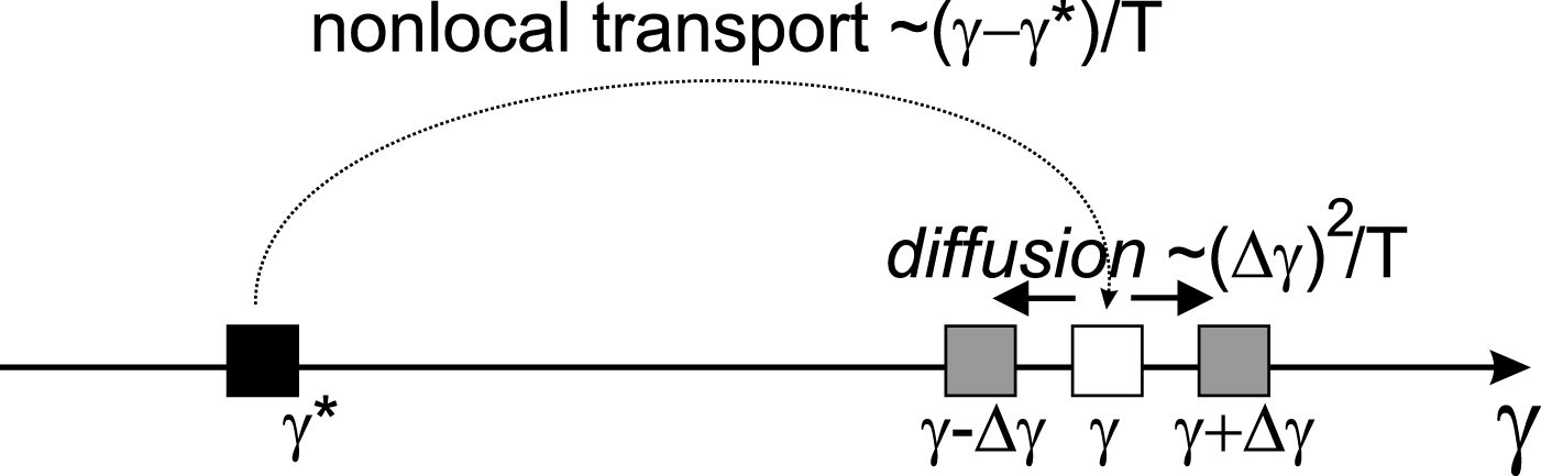
Reference Omura, Miyashita, Yoshikawa, Summers, Hikishima, Ebihara and Kubota2015). Such operators model the non-local relationships between different parts of the distribution in energy space: the particle distribution for a particular energy
 $\unicode[STIX]{x1D6FE}$
depends not only on its close surrounding, but also on the distribution at energy
 $\unicode[STIX]{x1D6FE}^{\ast }$
of trapped particles released from the resonance with energy
 $\unicode[STIX]{x1D6FE}$
(see scheme in figure 1). Although, there are several examples of these non-local operators derived numerically (Omura et al.
Reference Omura, Miyashita, Yoshikawa, Summers, Hikishima, Ebihara and Kubota2015) or analytically (Artemyev et al.
Reference Artemyev, Vasiliev, Mourenas, Agapitov, Krasnoselskikh, Boscher and Rolland2014), there is so far no unified approach for the derivation of a kinetic equation including all nonlinear effects. Recently, such an approach was proposed for simple one-dimensional systems with electrostatic waves (Artemyev et al.
Reference Artemyev, Neishtadt, Vasiliev and Mourenas2017b
) and we generalize it in the present paper to electromagnetic whistler mode waves propagating at an arbitrary angle relative to the background magnetic field.
Scheme of particle energy
 $\unicode[STIX]{x1D6FE}$
change over a time
 $T$
due to diffusion and due to non-local transport.

The paper is organized as follows: § 2.1 is devoted to general expressions of whistler mode wave electromagnetic fields through vector and scalar potentials; in § 2.2 we derive the general form of the Hamiltonian describing electron motion in an inhomogeneous (dipole) magnetic field and wave fields; in § 2.3 we expand this Hamiltonian around the wave–particle resonance and derive the resonant Hamiltonian describing resonant particle dynamics; in § 2.4 we use this resonant Hamiltonian to derive the main characteristics of resonant particle motion (change of energy due to trapping and due to scattering); § 3 is devoted to the derivation of a generalized kinetic equation describing the evolution of the particle distribution due to nonlinear resonant interactions; in §§ 4 and 5 we apply this equation to describe the evolution of the resonant electron distribution in a system with a parallel propagating whistler mode wave (cyclotron resonance) and in a system with a highly oblique whistler mode wave (Landau resonance); finally, we discuss in § 6 the main results and possible generalization/modifications of the derived equations.
2 Main system characteristics
This section consists of three subsections: § 2.1 describes the distribution of wave electromagnetic field and corresponding vector and scalar potentials, § 2.2 provides a Hamiltonian description of electron motion and § 2.3 outlines the main characteristics of wave–particle resonant interaction.
2.1 Wave field
The cold plasma dispersion relation (Stix Reference Stix1962) provides the relationship between electric and magnetic field components of whistler mode waves. Let
 $B_{y}=B_{w0}\text{Re}(\text{e}^{\text{i}\unicode[STIX]{x1D719}})=B_{w0}\cos \unicode[STIX]{x1D719}$
where
 $\unicode[STIX]{x1D719}$
is the wave phase, then
 $$\begin{eqnarray}\left.\begin{array}{@{}c@{}}{\displaystyle \frac{B_{x}}{B_{w0}}}=-\unicode[STIX]{x1D700}_{2}{\displaystyle \frac{N^{2}\sin ^{2}\unicode[STIX]{x1D703}-\unicode[STIX]{x1D700}_{3}}{\unicode[STIX]{x1D700}_{3}(\unicode[STIX]{x1D700}_{1}-N^{2})}}\sin \unicode[STIX]{x1D719},\quad {\displaystyle \frac{B_{z}}{B_{w0}}}=\tan \unicode[STIX]{x1D703}\unicode[STIX]{x1D700}_{2}{\displaystyle \frac{N^{2}\sin ^{2}\unicode[STIX]{x1D703}-\unicode[STIX]{x1D700}_{3}}{\unicode[STIX]{x1D700}_{3}(\unicode[STIX]{x1D700}_{1}-N^{2})}}\sin \unicode[STIX]{x1D719},\\ {\displaystyle \frac{E_{x}}{B_{w0}}}=-{\displaystyle \frac{N^{2}\sin ^{2}\unicode[STIX]{x1D703}-\unicode[STIX]{x1D700}_{3}}{\unicode[STIX]{x1D700}_{3}N\cos \unicode[STIX]{x1D703}}}\cos \unicode[STIX]{x1D719},\quad {\displaystyle \frac{E_{y}}{B_{w0}}}={\displaystyle \frac{\unicode[STIX]{x1D700}_{2}}{\unicode[STIX]{x1D700}_{1}-N^{2}}}{\displaystyle \frac{N^{2}\sin ^{2}\unicode[STIX]{x1D703}-\unicode[STIX]{x1D700}_{3}}{\unicode[STIX]{x1D700}_{3}N\cos \unicode[STIX]{x1D703}}}\sin \unicode[STIX]{x1D719},\\ {\displaystyle \frac{E_{z}}{B_{w0}}}=-{\displaystyle \frac{N\sin \unicode[STIX]{x1D703}}{\unicode[STIX]{x1D700}_{3}}}\cos \unicode[STIX]{x1D719}.\end{array}\right\}\end{eqnarray}$$
Functions
 $\unicode[STIX]{x1D700}_{1}$
,
 $\unicode[STIX]{x1D700}_{2}$
and
 $\unicode[STIX]{x1D700}_{3}$
are components of the cold plasma dielectric tensor:
 $$\begin{eqnarray}\unicode[STIX]{x1D700}_{1}=1-{\displaystyle \frac{\unicode[STIX]{x1D6FA}_{\text{pe}}^{2}}{\unicode[STIX]{x1D714}^{2}-\unicode[STIX]{x1D6FA}_{0}^{2}}},\quad \unicode[STIX]{x1D700}_{2}={\displaystyle \frac{\unicode[STIX]{x1D6FA}_{0}}{\unicode[STIX]{x1D714}}}{\displaystyle \frac{\unicode[STIX]{x1D6FA}_{\text{pe}}^{2}}{\unicode[STIX]{x1D714}^{2}-\unicode[STIX]{x1D6FA}_{0}^{2}}},\quad \unicode[STIX]{x1D700}_{3}=1-{\displaystyle \frac{\unicode[STIX]{x1D6FA}_{\text{pe}}^{2}}{\unicode[STIX]{x1D714}^{2}}},\end{eqnarray}$$
where
 $\unicode[STIX]{x1D714}$
is the wave frequency,
 $k_{x}$
and
 $k_{z}$
are two components of the wave vector lying in the
 $(x,z)$
plane (
 $k_{x}=k\sin \unicode[STIX]{x1D703}$
,
 $k_{z}=k\cos \unicode[STIX]{x1D703}$
),
 $\unicode[STIX]{x1D6FA}_{0}>0$
is the electron gyrofrequency in the background magnetic field directed along the
 $z$
axis,
 $\unicode[STIX]{x1D6FA}_{\text{pe}}$
the plasma frequency. Wave frequency and wave vector satisfy the wave dispersion relation
 $N=N(\unicode[STIX]{x1D714},\unicode[STIX]{x1D703})$
where
 $N=kc/\unicode[STIX]{x1D714}$
is the wave refractive index (Stix Reference Stix1962). Equations (2.1) lead to the following expressions for the total wave magnetic and electric fields:
 $$\begin{eqnarray}\displaystyle \left.\begin{array}{@{}c@{}}B_{w}^{2}={\displaystyle \frac{1}{2\unicode[STIX]{x03C0}}}\displaystyle \int _{0}^{2\unicode[STIX]{x03C0}}(B_{x}^{2}+B_{y}^{2}+B_{z}^{2})\,\text{d}\unicode[STIX]{x1D719}={\displaystyle \frac{1}{2}}B_{w0}^{2}(C_{2}C_{1}+1)\\ E_{w}^{2}={\displaystyle \frac{1}{2\unicode[STIX]{x03C0}}}\displaystyle \int _{0}^{2\unicode[STIX]{x03C0}}(E_{x}^{2}+E_{y}^{2}+E_{z}^{2})\,\text{d}\unicode[STIX]{x1D719}={\displaystyle \frac{1}{2}}{\displaystyle \frac{B_{w0}^{2}}{N^{2}}}(C_{1}(1+C_{2})+(N^{2}\unicode[STIX]{x1D700}_{3}^{-1}\sin \unicode[STIX]{x1D703})^{2})\\ C_{1}=\left({\displaystyle \frac{N^{2}\unicode[STIX]{x1D700}_{3}^{-1}\sin ^{2}\unicode[STIX]{x1D703}-1}{\cos \unicode[STIX]{x1D703}}}\right)^{2},\quad C_{2}=\left({\displaystyle \frac{\unicode[STIX]{x1D700}_{2}}{\unicode[STIX]{x1D700}_{1}-N^{2}}}\right)^{2}.\end{array}\right\} & & \displaystyle\end{eqnarray}$$
For parallel propagating waves (
 $\unicode[STIX]{x1D703}=0$
), we have
 $C_{1}=1$
,
 $N^{2}=\unicode[STIX]{x1D700}_{1}-\unicode[STIX]{x1D700}_{2}$
,
 $C_{2}=1$
and
 $B_{w}=B_{w0}$
,
 $E_{w}=B_{w0}/N$
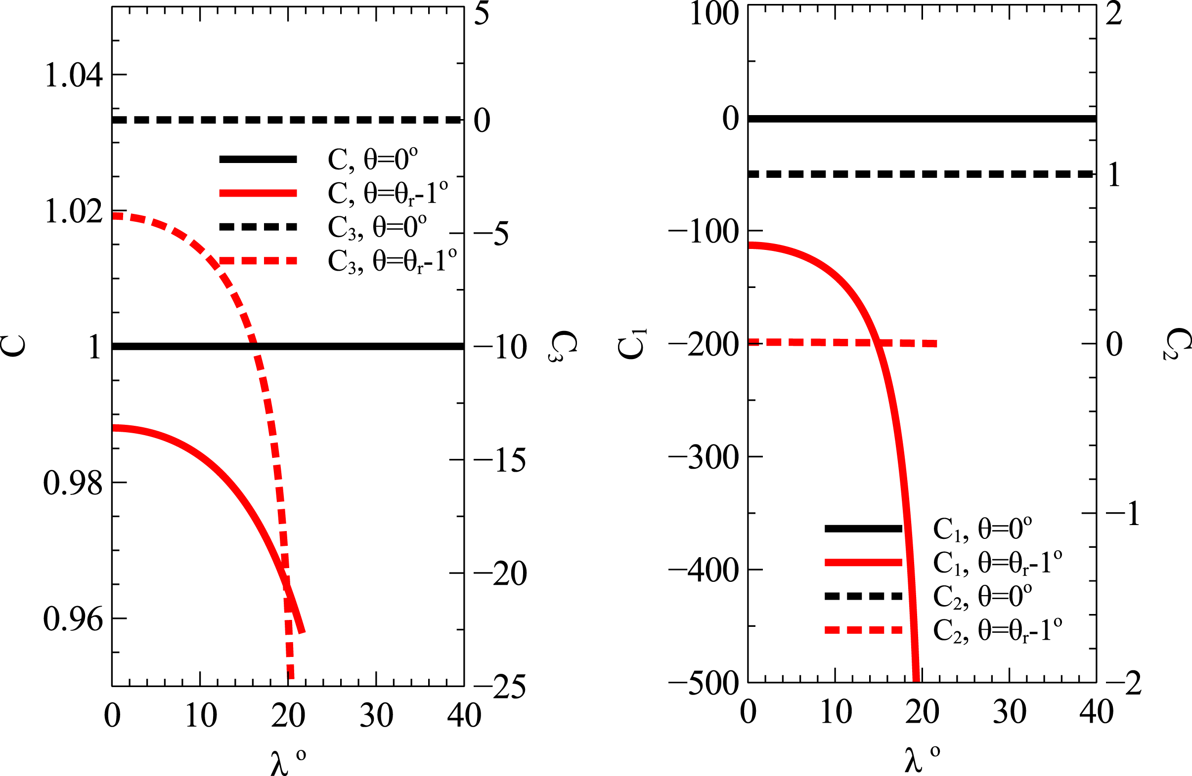
. Figure 2 shows the functions
 $C_{1}$
,
 $C_{2}$
for different parameters, corresponding notably to parallel and very oblique waves in the radiation belts.
Functions
 $C_{1}$
,
 $C_{2}$
given by (2.3), and functions
 $C=\sqrt{C_{1}C_{2}}$
,
 $C_{3}=(N^{2}\unicode[STIX]{x1D700}_{3}^{-1}-1)/$
 $N\cos \unicode[STIX]{x1D703}$
for
 $\unicode[STIX]{x1D714}/\unicode[STIX]{x1D6FA}_{0}=0.35$
and
 $\unicode[STIX]{x1D6FA}_{\text{pe}}/\unicode[STIX]{x1D6FA}_{0}=4.5$
at
 $\unicode[STIX]{x1D706}=0$
, considering field-aligned (
 $\unicode[STIX]{x1D703}=0$
) and highly oblique waves near the resonance cone angle
 $\unicode[STIX]{x1D703}_{r}$
.

We use the Coulomb gauge to write field components through components of vector potential
 $\boldsymbol{A}$
and scalar potential
 $\unicode[STIX]{x1D711}$
:
 $$\begin{eqnarray}\displaystyle \left.\begin{array}{@{}c@{}}A_{y}={\displaystyle \frac{B_{w0}}{k}}\sqrt{C_{2}C_{1}}\cos \unicode[STIX]{x1D719},\quad A_{x}={\displaystyle \frac{B_{w0}}{k}}\cos \unicode[STIX]{x1D703}\sin \unicode[STIX]{x1D719},\quad \\ A_{z}=-{\displaystyle \frac{B_{w0}}{k}}\sin \unicode[STIX]{x1D703}\sin \unicode[STIX]{x1D719},\quad \unicode[STIX]{x1D711}={\displaystyle \frac{B_{w0}}{kN}}(N^{2}\unicode[STIX]{x1D700}_{3}^{-1}-1)\tan \unicode[STIX]{x1D703}\sin \unicode[STIX]{x1D719}.\end{array}\right\} & & \displaystyle\end{eqnarray}$$
We introduce
 $A_{0}=B_{w0}/k$
,
 $C=\sqrt{C_{1}C_{2}}$
,
 $C_{3}=(N^{2}\unicode[STIX]{x1D700}_{3}^{-1}-1)/N\cos \unicode[STIX]{x1D703}$
and write
 $A_{x}=A_{0}\cos \unicode[STIX]{x1D703}\sin \unicode[STIX]{x1D719}$
,
 $A_{y}=A_{0}C\cos \unicode[STIX]{x1D719}$
,
 $A_{z}=-A_{0}\sin \unicode[STIX]{x1D703}\sin \unicode[STIX]{x1D719}$
,
 $\unicode[STIX]{x1D711}=A_{0}C_{3}\sin \unicode[STIX]{x1D703}\sin \unicode[STIX]{x1D719}$
where
 $B_{w0}=B_{w}\sqrt{2/(C^{2}+1)}$
. Figure 2 shows
 $C$
and
 $C_{3}\tan \unicode[STIX]{x1D703}$
as functions of the magnetic latitude
 $\unicode[STIX]{x1D706}$
for a dipole model of the background magnetic field (
 $\unicode[STIX]{x1D6FA}_{0}(\unicode[STIX]{x1D706})=\unicode[STIX]{x1D6FA}_{0}(0)\sqrt{1+3\sin ^{2}\unicode[STIX]{x1D706}}/\cos ^{6}\unicode[STIX]{x1D706}$
). Highly oblique waves, with
 $\unicode[STIX]{x1D703}$
close to the resonance cone angle
 $\unicode[STIX]{x1D703}_{r}$
(Stix Reference Stix1962), are characterized by a significant variation of vector and scalar potential amplitudes, whereas these amplitudes are almost constant for parallel propagating waves.
2.2 Electron dynamics
We start with the Hamiltonian of an electron (of charge
 $-e$
and mass
 $m_{e}$
) moving in the background magnetic field (described by the
 $y$
-component of the vector potential
 $A_{bg}=-xB_{0}(z)$
(Bell Reference Bell1984)) and the wave electromagnetic field (given by (2.4)):
 $$\begin{eqnarray}H=\sqrt{m_{e}^{2}c^{4}+c^{2}\left(\boldsymbol{p}+{\displaystyle \frac{e}{c}}\boldsymbol{A}(x,z,t)+{\displaystyle \frac{e}{c}}A_{bg}(x,z)\boldsymbol{e}_{y}\right)^{2}}-e\unicode[STIX]{x1D711}(x,z,t),\end{eqnarray}$$
where
 $\boldsymbol{p}$
is the particle generalized momentum. Note that
 $(x,y,z)$
are Cartesian coordinates, i.e. we do not take into account the magnetic field line curvature of the dipole field (see a more general consideration in Shklyar & Matsumoto Reference Shklyar and Matsumoto2009). Although we use a
 $B_{0}(z)$
function simulating the distribution of a dipole field along magnetic field line, the same consideration is valid for arbitrary ambient magnetic field with a sufficiently large spatial scale of inhomogeneity.
The Hamiltonian (2.5) does not depend on
 $y$
and the conjugated momentum is constant,
 $p_{y}=\text{const}$
. We consider particles motion around a field line with
 $x=0$
, and thus
 $p_{y}$
can be taken equal to zero. There are two important assumptions here. First, we assume that the spatial scale of the
 $B_{0}(z)$
variation is much larger than the wavelength
 ${\sim}(\unicode[STIX]{x2202}\unicode[STIX]{x1D719}/\unicode[STIX]{x2202}x)^{-1},\,(\unicode[STIX]{x2202}\unicode[STIX]{x1D719}/\unicode[STIX]{x2202}z)^{-1}$
. Therefore, the period of particle oscillations in the plane
 $(z,p_{z})$
are much longer than the wave period
 $\unicode[STIX]{x1D719}$
(wave frequency
 $-\unicode[STIX]{x2202}\unicode[STIX]{x1D719}/\unicode[STIX]{x2202}t$
is approximately the electron gyrofrequency
 $eB_{0}/m_{e}c$
and much larger than an inverted time scale of
 $(z,p_{z})$
oscillations). Second, we assume a small wave amplitude
 $eA_{0}/m_{e}c^{2}\ll 1$
(for typical conditions in the Earth radiation belts this limit is satisfied since it means that the wave magnetic field amplitude must be much smaller than
 $10$
nT) and expand the Hamiltonian (2.5) as:
 $$\begin{eqnarray}\left.\begin{array}{@{}c@{}}H=H_{0}+{\displaystyle \frac{ce}{H_{0}}}\boldsymbol{A}\left(\boldsymbol{p}+{\displaystyle \frac{e}{c}}A_{bg}\boldsymbol{e}_{y}\right)-e\unicode[STIX]{x1D711}\\ H_{0}=\sqrt{m_{e}^{2}c^{4}+c^{2}p_{z}^{2}+c^{2}p_{x}^{2}+c^{2}(m_{e}x\unicode[STIX]{x1D6FA}_{0}(z))^{2}},\end{array}\right\}\end{eqnarray}$$
where
 $\unicode[STIX]{x1D6FA}_{0}=eB_{0}(z)/m_{e}c$
. Considering the unperturbed system
 $H=H_{0}$
, we introduce the adiabatic invariant (magnetic moment):
 $$\begin{eqnarray}I_{x}={\displaystyle \frac{1}{2\unicode[STIX]{x03C0}}}\oint p_{x}\,\text{d}x={\displaystyle \frac{\mathop{H}_{0}^{2}-m_{e}^{2}c^{4}-c^{2}p_{z}^{2}}{2m_{e}c^{2}\unicode[STIX]{x1D6FA}_{0}}}.\end{eqnarray}$$
The corresponding coordinates
 $(x,p_{x})$
can be rewritten as:
 $p_{x}=-\sqrt{2I_{x}\unicode[STIX]{x1D6FA}_{0}m_{e}}\sin \unicode[STIX]{x1D713}$
and
 $x=\sqrt{2I_{x}/\unicode[STIX]{x1D6FA}_{0}m_{e}}\cos \unicode[STIX]{x1D713}$
where
 $I_{x},\unicode[STIX]{x1D713}$
are conjugated variables (i.e. the transformation
 $(x,p_{x})$
to
 $(\unicode[STIX]{x1D713},I_{x})$
is canonical (Landau & Lifshitz Reference Landau and Lifshitz1988)). To introduce these variables we use the generating function
 $G_{0}=\int p_{x}\,\text{d}x+p_{z,\text{new}}z$
where
 $$\begin{eqnarray}p_{z,\text{new}}=p_{z}-{\displaystyle \frac{\unicode[STIX]{x2202}G_{0}}{\unicode[STIX]{x2202}z}}=p_{z}-I_{x}{\displaystyle \frac{1}{2}}{\displaystyle \frac{\unicode[STIX]{x2202}\ln \unicode[STIX]{x1D6FA}_{0}}{\unicode[STIX]{x2202}z}}\sin 2\unicode[STIX]{x1D713}\end{eqnarray}$$
and
 $z$
does not change. Therefore, the Hamiltonian (2.6) can be rewritten in new variables:
 $$\begin{eqnarray}\displaystyle \hspace{-7.20007pt}\left.\begin{array}{@{}c@{}}H=m_{e}c^{2}\sqrt{1+{\displaystyle \frac{1}{m_{e}^{2}c^{2}}}\left(p_{z,\text{new}}+I_{x}{\displaystyle \frac{1}{2}}{\displaystyle \frac{\unicode[STIX]{x2202}\ln \unicode[STIX]{x1D6FA}_{0}}{\unicode[STIX]{x2202}z}}\sin 2\unicode[STIX]{x1D713}\right)^{2}+{\displaystyle \frac{\unicode[STIX]{x1D70C}^{2}\unicode[STIX]{x1D6FA}_{0}^{2}}{c^{2}}}}+H_{1},\\ H_{1}={\displaystyle \frac{1}{\unicode[STIX]{x1D6FE}_{0}}}\!\left(\!{\displaystyle \frac{\unicode[STIX]{x1D70C}\unicode[STIX]{x1D6FA}_{0}}{c}}(eA_{y}\cos \unicode[STIX]{x1D713}-eA_{x}\sin \unicode[STIX]{x1D713})+{\displaystyle \frac{eA_{z}}{m_{e}c}}\!\left(\!p_{z,\text{new}}+I_{x}{\displaystyle \frac{1}{2}}{\displaystyle \frac{\unicode[STIX]{x2202}\ln \unicode[STIX]{x1D6FA}_{0}}{\unicode[STIX]{x2202}z}}\sin 2\unicode[STIX]{x1D713}\right)\!\right)\!-e\unicode[STIX]{x1D711},\quad \end{array}\right\} & & \displaystyle \nonumber\\ \displaystyle & & \displaystyle\end{eqnarray}$$
where
 $\unicode[STIX]{x1D70C}=\sqrt{2I_{x}/m_{e}\unicode[STIX]{x1D6FA}_{0}}$
. There is a fast oscillating term
 ${\sim}\text{sin}\,2\unicode[STIX]{x1D713}$
. This term results in variation of adiabatic invariant
 $I_{x}$
(
 ${\dot{I}}_{x}=-\unicode[STIX]{x2202}H/\unicode[STIX]{x2202}\unicode[STIX]{x1D713}$
). The amplitude of this term is
 ${\sim}\unicode[STIX]{x2202}\ln \unicode[STIX]{x1D6FA}_{0}/\unicode[STIX]{x2202}z$
, i.e.
 $I_{x}$
is conserved with accuracy
 ${\sim}\unicode[STIX]{x2202}\ln \unicode[STIX]{x1D6FA}_{0}/\unicode[STIX]{x2202}z$
. In the absence of wave perturbations (i.e. in the absence of external forces depending on the wave phase
 $\unicode[STIX]{x1D719}$
) we can always introduce the improved adiabatic invariant
 $J_{x}$
, which is conserved with accuracy
 ${\sim}(\unicode[STIX]{x2202}\ln \unicode[STIX]{x1D6FA}_{0}/\unicode[STIX]{x2202}z)^{2}$
(Arnold Kozlov & Neishtadt Reference Arnold, Kozlov and Neishtadt2006). In a system with the wave depending on the phase
 $\unicode[STIX]{x1D719}$
, the variation of
 $I_{x}$
is determined by the resonance of the wave phase
 $n\unicode[STIX]{x1D713}+\unicode[STIX]{x1D719}$
,
 $n=0,\pm 1,\pm 2,\ldots$
(see below). For resonant particles with
 $\text{d}(n\unicode[STIX]{x1D713}+\unicode[STIX]{x1D719})/\text{d}t\approx 0$
the phase
 $2\unicode[STIX]{x1D713}$
is a fast oscillating non-resonant phase, and, after expansion of
 $\unicode[STIX]{x1D6FE}_{\text{new}}$
over
 $\unicode[STIX]{x2202}\ln \unicode[STIX]{x1D6FA}_{0}/\unicode[STIX]{x2202}z$
, the corresponding term
 ${\sim}\text{sin}\,2\unicode[STIX]{x1D713}$
can be omitted as a fast oscillating term with mean zero value. Therefore, we can rewrite the Hamiltonian (2.9) as
 $$\begin{eqnarray}\displaystyle \left.\begin{array}{@{}c@{}}H=m_{e}c^{2}\unicode[STIX]{x1D6FE}+H_{1},\;\unicode[STIX]{x1D6FE}=\sqrt{1+{\displaystyle \frac{p_{z}^{2}}{m_{e}^{2}c^{2}}}+{\displaystyle \frac{\unicode[STIX]{x1D70C}^{2}\unicode[STIX]{x1D6FA}_{0}^{2}}{c^{2}}}}\\ H_{1}={\displaystyle \frac{1}{\unicode[STIX]{x1D6FE}}}\left({\displaystyle \frac{\unicode[STIX]{x1D70C}\unicode[STIX]{x1D6FA}_{0}}{c}}(eA_{y}\cos \unicode[STIX]{x1D713}-eA_{x}\sin \unicode[STIX]{x1D713})+{\displaystyle \frac{eA_{z}}{m_{e}c}}p_{z}\right)-e\unicode[STIX]{x1D711},\end{array}\right\} & & \displaystyle\end{eqnarray}$$
were
 $p_{z,\text{new}}\approx p_{z}$
.
We then substitute equations (2.4) into the
 $H_{1}$
expression to get:
 $$\begin{eqnarray}\displaystyle & H_{1}={\displaystyle \frac{eA_{0}}{\unicode[STIX]{x1D6FE}}}{\displaystyle \frac{\unicode[STIX]{x1D70C}\unicode[STIX]{x1D6FA}_{0}}{c}}(C\cos \unicode[STIX]{x1D719}\cos \unicode[STIX]{x1D713}-\cos \unicode[STIX]{x1D703}\sin \unicode[STIX]{x1D719}\sin \unicode[STIX]{x1D713})-eA_{0}\left({\displaystyle \frac{p_{z}}{\unicode[STIX]{x1D6FE}m_{e}c}}+C_{3}\right)\sin \unicode[STIX]{x1D703}\sin \unicode[STIX]{x1D719}, & \displaystyle \nonumber\\ \displaystyle & & \displaystyle\end{eqnarray}$$
where wave phase
 $\unicode[STIX]{x1D719}$
can be written as
 $$\begin{eqnarray}\unicode[STIX]{x1D719}=\unicode[STIX]{x1D719}_{\Vert }+k_{x}\unicode[STIX]{x1D70C}\cos \unicode[STIX]{x1D713},\quad \unicode[STIX]{x1D719}_{\Vert }=\displaystyle \int _{}^{z}k_{z}(\tilde{z})\,\text{d}\tilde{z}-\unicode[STIX]{x1D714}t.\end{eqnarray}$$
Using the Jacobi–Anger expansion, we rewrite (2.11) as
 $$\begin{eqnarray}\displaystyle \left.\begin{array}{@{}rcl@{}}H_{1}\, & =\, & eA_{0}\displaystyle \mathop{\sum }_{n=-\infty }^{\infty }h^{(n)}(I_{x},p_{z},z)\sin \left(\unicode[STIX]{x1D719}_{\Vert }+n{\displaystyle \frac{\unicode[STIX]{x03C0}}{2}}-n\unicode[STIX]{x1D713}\right)\\ h^{(n)}\, & =\, & {\displaystyle \frac{\unicode[STIX]{x1D70C}\unicode[STIX]{x1D6FA}_{0}}{2c\unicode[STIX]{x1D6FE}}}((C-\cos \unicode[STIX]{x1D703})J_{n-1}(k_{x}\unicode[STIX]{x1D70C})-(C+\cos \unicode[STIX]{x1D703})J_{n+1}(k_{x}\unicode[STIX]{x1D70C}))\\ \, & \, & -\,\left({\displaystyle \frac{p_{z}}{\unicode[STIX]{x1D6FE}m_{e}c}}+C_{3}\right)\sin \unicode[STIX]{x1D703}J_{n}(k_{x}\unicode[STIX]{x1D70C}),\end{array}\right\} & & \displaystyle\end{eqnarray}$$
where
 $J_{n}$
is the Bessel function. We consider waves with insufficiently strong amplitudes to allow an overlap of resonances, i.e. such that each term in the sum of resonances can be considered independently (i.e. the resonance width
 ${\sim}\sqrt{|eA_{0}h^{(n)}/m_{e}|}$
is much smaller than the smallest distance between two resonances
 ${\sim}\unicode[STIX]{x1D6FA}_{0}/k\cos \unicode[STIX]{x1D703}$
, see the corresponding discussion in Shklyar Reference Shklyar1981). For one particular
 $n$
, equation (2.10) takes the form
 $$\begin{eqnarray}H^{(n)}=m_{e}c^{2}\unicode[STIX]{x1D6FE}+eA_{0}h^{(n)}\sin \left(\unicode[STIX]{x1D719}_{\Vert }+n{\displaystyle \frac{\unicode[STIX]{x03C0}}{2}}-n\unicode[STIX]{x1D713}\right).\end{eqnarray}$$
Numerically solving the Hamiltonian equations for the
 $(z,p_{z})$
,
 $(\unicode[STIX]{x1D713},I_{x})$
variables for the Hamiltonian (2.14) allows us to describe the resonant interaction of charged particles with a whistler mode wave. In the next subsection, we investigate the Hamiltonian (2.14) to determine the main characteristics of this resonant interaction.
2.3 Wave–particle resonance
First, we would like to consider a conservative system with conserved energy, whereas the Hamiltonian (2.14) depends on time through phase
 $\unicode[STIX]{x1D719}_{\Vert }$
. To exclude this temporal dependence, we introduce the new conjugated variables
 $(\unicode[STIX]{x1D701}_{n},I)$
and
 $(z,P_{z})$
with
 $\unicode[STIX]{x1D701}_{n}=\unicode[STIX]{x1D719}_{\Vert }-n\unicode[STIX]{x1D713}+n\unicode[STIX]{x03C0}/2$
. This variable change excludes phase
 $\unicode[STIX]{x1D713}$
from the Hamiltonian and, thus, the new momentum
 $\tilde{I_{x}}$
is constant – i.e. instead of two pairs of conjugated variables
 $(z,p_{z})$
,
 $(\unicode[STIX]{x1D713},I_{x})$
we introduce
 $(z,P_{z})$
,
 $(\unicode[STIX]{x1D701}_{n},I)$
. To this aim, we use the generating function
 $G_{1}=(\unicode[STIX]{x1D719}_{\Vert }+n\unicode[STIX]{x1D713}+n\unicode[STIX]{x03C0}/2)I+zP_{z}+\unicode[STIX]{x1D713}\tilde{I} _{x}$
corresponding to:
 $$\begin{eqnarray}\unicode[STIX]{x1D701}_{n}=\unicode[STIX]{x1D719}_{\Vert }+n{\displaystyle \frac{\unicode[STIX]{x03C0}}{2}}-n\unicode[STIX]{x1D713},\quad p_{z}=k_{z}I+P_{z},\quad I_{x}=-nI+\tilde{I} _{x}.\end{eqnarray}$$
Therefore, the new Hamiltonian
 $F=H^{(n)}+\unicode[STIX]{x2202}G_{1}/\unicode[STIX]{x2202}t$
takes the form
 $$\begin{eqnarray}\displaystyle \left.\begin{array}{@{}c@{}}F=-\unicode[STIX]{x1D714}I+m_{e}c^{2}\unicode[STIX]{x1D6FE}+eA_{0}h^{(n)}\sin \unicode[STIX]{x1D701}_{n}\\ \unicode[STIX]{x1D6FE}=\sqrt{1+{\displaystyle \frac{(k_{z}I+P_{z})^{2}}{m_{e}^{2}c^{2}}}+{\displaystyle \frac{2\unicode[STIX]{x1D6FA}_{0}}{m_{e}c^{2}}}(\tilde{I} _{x}-nI)},\end{array}\right\} & & \displaystyle\end{eqnarray}$$
where
 $h^{(n)}=h^{(n)}(\tilde{I} _{x}-nI,k_{z}I+P_{z},z)$
. The resonance condition
 $\dot{\unicode[STIX]{x1D701}}_{n}=0$
can be written through Hamiltonian equations:
 $$\begin{eqnarray}\dot{\unicode[STIX]{x1D701}}_{n}={\displaystyle \frac{\unicode[STIX]{x2202}F}{\unicode[STIX]{x2202}I}}=-\unicode[STIX]{x1D714}+{\displaystyle \frac{k_{z}(k_{z}I+P_{z})-m_{e}\unicode[STIX]{x1D6FA}_{0}n}{m_{e}\unicode[STIX]{x1D6FE}}}=0,\end{eqnarray}$$
where we omit perturbations
 ${\sim}eA_{0}\ll m_{e}c^{2}$
. The solution of (2.17) provides the resonant value
 $I_{R}$
of momentum
 $I$
:
 $$\begin{eqnarray}{\displaystyle \frac{k_{z}I_{R}}{m_{e}c}}=-{\displaystyle \frac{P_{z}}{m_{e}c}}-{\displaystyle \frac{\unicode[STIX]{x1D714}_{n}}{N_{\Vert }}}+{\displaystyle \frac{1}{\sqrt{N_{\Vert }^{2}-1}}}\sqrt{1+\unicode[STIX]{x1D6FD}_{\bot }^{2}-{\displaystyle \frac{\unicode[STIX]{x1D714}_{n}^{2}}{N_{\Vert }^{2}}}-2{\displaystyle \frac{\unicode[STIX]{x1D714}_{n}}{N_{\Vert }}}{\displaystyle \frac{P_{z}}{m_{e}c}}},\end{eqnarray}$$
where
 $N_{\Vert }=k_{z}c/\unicode[STIX]{x1D714}$
,
 $\unicode[STIX]{x1D714}_{n}=-n\unicode[STIX]{x1D6FA}_{0}/\unicode[STIX]{x1D714}$
, and
 $\unicode[STIX]{x1D6FD}_{\bot }=\sqrt{2\tilde{I} _{x}\unicode[STIX]{x1D6FA}_{0}/m_{e}c^{2}}$
. Particles with
 $I=I_{R}$
are in resonance with the wave. Therefore, to consider such resonant particles we expand the Hamiltonian (2.4) around
 $I_{R}$
:
 $$\begin{eqnarray}\displaystyle \left.\begin{array}{@{}c@{}}F=\unicode[STIX]{x1D6EC}+{\displaystyle \frac{1}{2}}m_{e}c^{2}g(I-I_{R})^{2}+eA_{0}h_{R}^{(n)}\sin \unicode[STIX]{x1D701}_{n}\\ \unicode[STIX]{x1D6EC}=-\unicode[STIX]{x1D714}I_{R}+m_{e}c^{2}\unicode[STIX]{x1D6FE}_{R}={\displaystyle \frac{m_{e}c^{2}}{N_{\Vert }^{2}}}\left({\displaystyle \frac{N_{\Vert }P_{z}}{m_{e}c}}+\unicode[STIX]{x1D714}_{n}+(N_{\Vert }^{2}-1)\unicode[STIX]{x1D6FE}_{R}\right)\\ \unicode[STIX]{x1D6FE}_{R}={\displaystyle \frac{N_{\Vert }}{\sqrt{N_{\Vert }^{2}-1}}}\sqrt{1+\unicode[STIX]{x1D6FD}_{\bot }^{2}-{\displaystyle \frac{\unicode[STIX]{x1D714}_{n}^{2}}{N_{\Vert }^{2}}}-2{\displaystyle \frac{\unicode[STIX]{x1D714}_{n}}{N_{\Vert }}}{\displaystyle \frac{P_{z}}{m_{e}c}}}\\ g=\left.{\displaystyle \frac{\unicode[STIX]{x2202}^{2}\unicode[STIX]{x1D6FE}}{\unicode[STIX]{x2202}I^{2}}}\right|_{I=I_{R}}=(N_{\Vert }^{2}-1){\displaystyle \frac{\unicode[STIX]{x1D714}^{2}}{m_{e}^{2}c^{4}\unicode[STIX]{x1D6FE}_{R}}},\end{array}\right\} & & \displaystyle\end{eqnarray}$$
where
 $h_{R}^{(h)}=h^{(n)}(nI_{R}+\tilde{I} _{x},k_{z}I_{R}+P_{z},z)$
. We introduce variables
 $K=I-I_{R}$
,
 $p$
,
 $s$
through the generating function
 $G_{2}=(I-I_{R})\unicode[STIX]{x1D701}_{n}+P_{z}s$
(we keep the old notation for
 $\unicode[STIX]{x1D701}_{n}$
, because this transformation does not change the phase):
 $$\begin{eqnarray}K=I-I_{R},\quad p=P_{z}-{\displaystyle \frac{\unicode[STIX]{x2202}I_{R}}{\unicode[STIX]{x2202}z}}\unicode[STIX]{x1D701}_{n},\quad s=z+{\displaystyle \frac{\unicode[STIX]{x2202}I_{R}}{\unicode[STIX]{x2202}P_{z}}}\unicode[STIX]{x1D701}_{n}.\end{eqnarray}$$
The new Hamiltonian
 $W=\unicode[STIX]{x1D6EC}(s,p)+m_{e}c^{2}g(s,p)K^{2}/2+eA_{0}h_{R}^{(n)}(s,p)\sin \unicode[STIX]{x1D701}_{n}$
contains the
 $\unicode[STIX]{x1D6EC}$
function depending on
 $(s,p)$
. Terms
 ${\sim}\unicode[STIX]{x2202}I_{R}/\unicode[STIX]{x2202}z$
,
 $\unicode[STIX]{x2202}I_{R}/\unicode[STIX]{x2202}P_{z}$
in (2.20) are much smaller than
 $(z,P_{z})$
terms due to the condition
 $\unicode[STIX]{x2202}/\unicode[STIX]{x2202}z\ll k_{z}$
. Therefore, we can expand the function
 $\unicode[STIX]{x1D6EC}$
:
 $$\begin{eqnarray}\displaystyle & \hspace{-6.0pt}\unicode[STIX]{x1D6EC}(z,P_{z})=\unicode[STIX]{x1D6EC}\!\left(\!s-{\displaystyle \frac{\unicode[STIX]{x2202}I_{R}}{\unicode[STIX]{x2202}P_{z}}}\unicode[STIX]{x1D701}_{n},p+{\displaystyle \frac{\unicode[STIX]{x2202}I_{R}}{\unicode[STIX]{x2202}z}}\unicode[STIX]{x1D701}_{n}\right)=\unicode[STIX]{x1D6EC}(s,p)+\!\left({\displaystyle \frac{\unicode[STIX]{x2202}I_{R}}{\unicode[STIX]{x2202}P_{z}}}{\displaystyle \frac{\unicode[STIX]{x2202}\unicode[STIX]{x1D6EC}}{\unicode[STIX]{x2202}z}}-{\displaystyle \frac{\unicode[STIX]{x2202}I_{R}}{\unicode[STIX]{x2202}z}}{\displaystyle \frac{\unicode[STIX]{x2202}\unicode[STIX]{x1D6EC}}{\unicode[STIX]{x2202}P_{z}}}\right)\!\unicode[STIX]{x1D701}_{n}=\unicode[STIX]{x1D6EC}-r\unicode[STIX]{x1D701}_{n}, & \displaystyle \nonumber\\ \displaystyle & & \displaystyle\end{eqnarray}$$
where
 $r=\{\unicode[STIX]{x1D6EC},I_{R}\}_{z,P_{z}}\approx \{\unicode[STIX]{x1D6EC},I_{R}\}_{s,p}$
. Therefore, the new Hamiltonian
 $W$
can be split into two Hamiltonians
 $W=W_{\text{slow}}+\mathfrak{F}$
, where
 $W_{\text{slow}}=\unicode[STIX]{x1D6EC}(s,p)\sim m_{e}c^{2}$
describes the slow evolution of the
 $(s,p)$
variables, while
 $\mathfrak{F}\sim eA_{0}\ll m_{e}c^{2}$
depends on these variables as on the parameters and describes the fast variations of
 $(\unicode[STIX]{x1D701}_{n},K)$
:
 $$\begin{eqnarray}\displaystyle \left.\begin{array}{@{}c@{}}\mathfrak{F}={\displaystyle \frac{1}{2}}{\displaystyle \frac{N_{\Vert }^{2}-1}{\unicode[STIX]{x1D6FE}_{R}}}{\displaystyle \frac{\unicode[STIX]{x1D714}^{2}}{m_{e}^{2}c^{4}}}K^{2}-r\unicode[STIX]{x1D701}_{n}+eA_{0}h_{R}^{(n)}\sin \unicode[STIX]{x1D701}_{n}\\ r={\displaystyle \frac{m_{e}c^{2}DN_{\Vert }^{2}}{N_{\Vert }^{2}-1}}{\displaystyle \frac{1}{\unicode[STIX]{x1D6FE}_{R}}}\left({\displaystyle \frac{(\unicode[STIX]{x1D6FE}_{R}-\unicode[STIX]{x1D714}_{n})^{2}}{N_{\Vert }^{2}}}{\displaystyle \frac{\unicode[STIX]{x2202}\ln N_{\Vert }}{\unicode[STIX]{x2202}\ln \unicode[STIX]{x1D6FA}_{0}}}+{\displaystyle \frac{\unicode[STIX]{x1D714}_{n}}{N_{\Vert }}}{\displaystyle \frac{p}{m_{e}c}}-{\displaystyle \frac{1}{2}}\unicode[STIX]{x1D6FD}_{\bot }^{2}\right),\end{array}\right\} & & \displaystyle\end{eqnarray}$$
where
 $D=c(\unicode[STIX]{x2202}\ln \unicode[STIX]{x1D6FA}_{0}/\unicode[STIX]{x2202}s)/N_{\Vert }\unicode[STIX]{x1D714}\ll 1$
is a dimensionless factor determining the scale ratio of the inhomogeneity scale
 ${\sim}(\unicode[STIX]{x2202}/\unicode[STIX]{x2202}z)^{-1}$
and wavelength scale
 ${\sim}1/k_{z}$
.
2.4 Characteristics of resonant interaction
Using the resonant Hamiltonian (2.22), we can derive the main characteristics of the corresponding resonant wave–particle interaction. We start with the determination of values
 $(s,p)$
where the particle reaches resonance with the wave. Each particle trajectory is characterized by two constants: the generalized energy
 $\unicode[STIX]{x1D6FE}-\unicode[STIX]{x1D714}I/m_{e}c^{2}=\text{const.}$
(i.e. the normalized value of
 $F$
from (2.16) omitting small terms) and
 $\tilde{I} _{x}$
. Momenta
 $\tilde{I} _{x}$
and
 $I$
are linearly related to each other (
 $\tilde{I} _{x}=nI+I_{x}$
) and we define constant
 $\tilde{I} _{x}$
to be equal to the initial
 $I_{x}$
. Thus, the initial value of
 $I$
equals zero and
 $\unicode[STIX]{x1D6FE}_{\text{init}}=-\unicode[STIX]{x1D714}I_{R}/m_{e}c^{2}+\unicode[STIX]{x1D6FE}_{R}$
, where
 $\unicode[STIX]{x1D6FE}_{\text{init}}$
is the initial value of the energy. We substitute this equation into (2.18) and solve the obtained equation relative to resonant momentum
 $p_{R}\approx P_{z}$
:
 $$\begin{eqnarray}{\displaystyle \frac{p_{R}}{m_{e}c}}=N_{\Vert }\unicode[STIX]{x1D6FE}_{\text{init}}-N_{\Vert }\unicode[STIX]{x1D714}_{n}\pm \sqrt{N_{\Vert }^{2}-1}\sqrt{1+\unicode[STIX]{x1D700}+\unicode[STIX]{x1D714}_{n}^{2}},\end{eqnarray}$$
where we introduce a new function
 $\unicode[STIX]{x1D700}=\unicode[STIX]{x1D6FD}_{\bot }^{2}-2\unicode[STIX]{x1D6FE}_{\text{init}}\unicode[STIX]{x1D714}_{n}$
. For every
 $\unicode[STIX]{x1D6FE}_{\text{init}}$
, equation (2.23) defines the resonant curve
 $p_{R}=p_{R}(s)$
. The particles trapped into the resonance move along such curves, and thus particle energy
 $\unicode[STIX]{x1D6FE}=\unicode[STIX]{x1D6FE}_{R}$
and all coefficients of (2.22) can be rewritten as functions of
 $s$
only (i.e.
 $\unicode[STIX]{x1D714}_{n}(s)$
,
 $N_{\Vert }(s)$
):
 $$\begin{eqnarray}\displaystyle \left.\begin{array}{@{}c@{}}\unicode[STIX]{x1D6FE}=\left|\unicode[STIX]{x1D714}_{n}-{\displaystyle \frac{N_{\Vert }}{\sqrt{N_{\Vert }^{2}-1}}}\sqrt{1+\unicode[STIX]{x1D700}+\unicode[STIX]{x1D714}_{n}^{2}}\right|\\ {\displaystyle \frac{p_{R}}{m_{e}c}}=N_{\Vert }\unicode[STIX]{x1D6FE}_{\text{init}}-N_{\Vert }\unicode[STIX]{x1D714}_{n}\pm \sqrt{N_{\Vert }^{2}-1}\sqrt{1+\unicode[STIX]{x1D700}+\unicode[STIX]{x1D714}_{n}^{2}}\\ r={\displaystyle \frac{1}{2}}{\displaystyle \frac{m_{e}c^{2}DN_{\Vert }^{2}}{N_{\Vert }^{2}-1}}{\displaystyle \frac{1}{\unicode[STIX]{x1D6FE}}}\left(1-\unicode[STIX]{x1D6FE}^{2}+2{\displaystyle \frac{(\unicode[STIX]{x1D6FE}-\unicode[STIX]{x1D714}_{n})^{2}}{N_{\Vert }^{2}}}{\displaystyle \frac{\unicode[STIX]{x2202}\ln N_{\Vert }}{\unicode[STIX]{x2202}\ln \unicode[STIX]{x1D6FA}_{0}}}+{\displaystyle \frac{\unicode[STIX]{x1D6FE}^{2}-\unicode[STIX]{x1D714}_{n}^{2}}{N_{\Vert }^{2}}}\right).\end{array}\right\} & & \displaystyle\end{eqnarray}$$
The resonant coordinate
 $s_{R}(\unicode[STIX]{x1D6FE})$
is defined from the first equation of (2.24). Substituting
 $s_{R}(\unicode[STIX]{x1D6FE})$
to (2.22) and fixing
 $\tilde{I} _{x}$
, we obtain
 $r=r(\unicode[STIX]{x1D6FE})$
.
Defining resonant
 $p_{R}=p_{R}(\unicode[STIX]{x1D6FE},s_{R})$
and
 $s_{R}=s_{R}(\unicode[STIX]{x1D6FE})$
(see (2.23), (2.24)), we can provide a quantitative description of the particle resonant interaction. Let us start with the time scale between two successive resonance crossings,
 $T$
. We assume that there is one resonant interaction per period of slow
 $(z,p_{z})$
motion, i.e. the wave propagates from
 $z=0$
to positive
 $z$
and there is no wave at negative
 $z$
. This assumption also means that waves generated at
 $z=0$
and propagating to high
 $z$
are not reflected at high
 $z$
and do not return back to
 $z=0$
. Spacecraft observations (e.g. Agapitov et al.
Reference Agapitov, Krasnoselskikh, Zaliznyak, Angelopoulos, Le Contel and Rolland2011) and chorus wave modelling including the Landau damping effect (e.g. Bortnik et al.
Reference Bortnik, Inan and Bell2006; Breuillard et al.
Reference Breuillard, Zaliznyak, Agapitov, Artemyev, Krasnoselskikh and Rolland2013; Chen et al.
Reference Chen, Thorne, Li and Bortnik2013) suggest that in the Earth’s radiation belt, strong damping at high
 $z$
and spreading of wave power result in a very small intensity of the waves propagating back from high
 $z$
toward the
 $z=0$
plane. Thus,
 $T$
can be calculated from the unperturbed Hamiltonian (2.14):
 $$\begin{eqnarray}T(\unicode[STIX]{x1D6FE},\tilde{I} _{x})=\oint {\displaystyle \frac{\text{d}z}{\unicode[STIX]{x2202}H/\unicode[STIX]{x2202}p_{z}}}={\displaystyle \frac{\unicode[STIX]{x1D6FE}}{\sqrt{\unicode[STIX]{x1D6FE}^{2}-1}}}\oint \left(1-{\displaystyle \frac{\unicode[STIX]{x1D700}+2\unicode[STIX]{x1D714}_{n}\unicode[STIX]{x1D6FE}}{\unicode[STIX]{x1D6FE}^{2}-1}}\right)^{-1/2}{\displaystyle \frac{\text{d}z}{c}},\end{eqnarray}$$
where we rewrite
 $I_{x}=-nI+\tilde{I} _{x}$
through
 $\tilde{I} _{x}=\text{const.}$
,
 $-\unicode[STIX]{x1D714}I/m_{e}c^{2}+\unicode[STIX]{x1D6FE}=\unicode[STIX]{x1D6FE}_{\text{init}}$
, and
 $\unicode[STIX]{x1D700}=\unicode[STIX]{x1D6FA}_{0}\tilde{I} _{x}/m_{e}c^{2}-2\unicode[STIX]{x1D6FE}_{\text{init}}\unicode[STIX]{x1D714}_{n}$
. The period (2.25) depends only on the energy
 $\unicode[STIX]{x1D6FE}$
. The assumption that there is a single resonance during one bounce period does not follow from the system properties; it is used to simplify the derived equations. In more realistic systems, charged particles can resonate with the same wave several times along the bounce trajectory, and such multi-resonances can significantly influence charged particle motion (e.g. Shklyar Reference Shklyar1981). To include the effects of several resonances within one bounce period, we would need to describe the time scale between two successive resonances depending on the wave characteristics. This generalization of the derived equations will be considered in a future study.
Over one period
 $T$
, particle scattering results in a change of momentum
 $I$
, and a corresponding change of energy
 $\unicode[STIX]{x1D6FE}$
:
 $\unicode[STIX]{x1D714}\unicode[STIX]{x0394}I/m_{e}c^{2}=\unicode[STIX]{x0394}\unicode[STIX]{x1D6FE}$
: this change can be written as
 $$\begin{eqnarray}\displaystyle \left.\begin{array}{@{}rcl@{}}\unicode[STIX]{x0394}\unicode[STIX]{x1D6FE}\, & =\, & {\displaystyle \frac{\unicode[STIX]{x1D714}\unicode[STIX]{x0394}I}{m_{e}c^{2}}}=-{\displaystyle \frac{\unicode[STIX]{x1D714}}{m_{e}c^{2}}}\displaystyle \int {\displaystyle \frac{\unicode[STIX]{x2202}F}{\unicode[STIX]{x2202}\unicode[STIX]{x1D701}_{n}}}\,\text{d}t=-{\displaystyle \frac{2eA_{0}h_{R}^{(n)}\unicode[STIX]{x1D714}}{m_{e}c^{2}}}\displaystyle \int _{-\infty }^{\unicode[STIX]{x1D701}_{n}^{\ast }}{\displaystyle \frac{\cos \unicode[STIX]{x1D701}_{n}\,\text{d}\unicode[STIX]{x1D701}_{n}}{\dot{\unicode[STIX]{x1D701}}_{n}}}\\ \, & =\, & \sqrt{{\displaystyle \frac{2eA_{0}\unicode[STIX]{x1D6FE}_{R}h_{R}^{(n)}}{m_{e}c^{2}(N_{\Vert }^{2}-1)}}}f(\unicode[STIX]{x1D701}_{n}^{\ast },a)\\ f(\unicode[STIX]{x1D701}_{n}^{\ast },a)\, & =\, & \displaystyle \int _{-\infty }^{\unicode[STIX]{x1D701}_{n}^{\ast }}{\displaystyle \frac{\sqrt{a}\cos \unicode[STIX]{x1D701}_{n}\,\text{d}\unicode[STIX]{x1D701}_{n}}{\sqrt{\unicode[STIX]{x1D701}_{n}-\unicode[STIX]{x1D701}_{n}^{\ast }+a(\sin \unicode[STIX]{x1D701}_{n}^{\ast }-\sin \unicode[STIX]{x1D701}_{n})}}},\end{array}\right\} & & \displaystyle\end{eqnarray}$$
where the integration is performed along the trajectory of particles approaching the resonance from infinity, interacting with waves with the resonance value of phase
 $\unicode[STIX]{x1D701}_{n}^{\ast }$
and escaping from the resonance toward infinity. Note that integral (2.26) is written for negative
 $r$
(
 $\unicode[STIX]{x1D701}_{n}$
changes from
 $-\infty$
to
 $\unicode[STIX]{x1D701}_{n}^{\ast }$
), whereas for positive
 $r$
the integration should be performed for
 $\unicode[STIX]{x1D701}_{n}\in [\unicode[STIX]{x1D701}_{n}^{\ast },-\infty ]$
. The parameter
 $a=eA_{0}h_{R}^{(n)}/r$
and other parameters should be evaluated at
 $(p_{R},s_{R})$
, i.e. all these parameters depend only on
 $\unicode[STIX]{x1D6FE}$
. We further introduce the new variable
 $\unicode[STIX]{x1D709}$
through the particle energy evaluated at
 $\unicode[STIX]{x1D701}_{n}^{\ast }$
:
 $2\unicode[STIX]{x03C0}\unicode[STIX]{x1D709}=a\sin \unicode[STIX]{x1D701}_{n}^{\ast }-\unicode[STIX]{x1D701}_{n}^{\ast }$
. The function
 $f(\unicode[STIX]{x1D701}_{n}^{\ast },a)=f(\unicode[STIX]{x1D709},a)$
is a periodic function of
 $\unicode[STIX]{x1D709}$
, whereas
 $\unicode[STIX]{x1D709}$
depends on the initial value of
 $\unicode[STIX]{x1D701}_{n}$
and on the initial particle gyrophase (see, e.g. Karpman, Istomin & Shklyar Reference Karpman, Istomin and Shklyar1975). We do not include any information about particle gyrophase in our present description. Thus, we calculate here the average value of
 $f$
over
 $\unicode[STIX]{x1D709}$
. The distribution of
 $\unicode[STIX]{x1D709}$
is assumed to be uniform
 $\unicode[STIX]{x1D709}\in [0,1]$
(see corresponding numerical tests in Itin, Neishtadt & Vasiliev Reference Itin, Neishtadt and Vasiliev2000). An interesting and crucial property of the function
 $f(\unicode[STIX]{x1D709},a)$
is that
 $\langle \unicode[STIX]{x0394}I\rangle _{\unicode[STIX]{x1D709}}=-S_{\text{sep}}/2\unicode[STIX]{x03C0}$
(Karpman et al.
Reference Karpman, Istomin and Shklyar1975; Neishtadt Reference Neishtadt and Sim1999; Dolgopyat Reference Dolgopyat2012) where
 $S_{\text{sep}}$
is defined as:
 $$\begin{eqnarray}S_{\text{sep}}=\oint K\,\text{d}\unicode[STIX]{x1D701}_{n}=2^{3/2}\sqrt{{\displaystyle \frac{\unicode[STIX]{x1D6FE}_{R}r}{N_{\Vert }^{2}-1}}{\displaystyle \frac{m_{e}^{2}c^{4}}{\unicode[STIX]{x1D714}^{2}}}}\displaystyle \int _{\unicode[STIX]{x1D701}_{\min }}^{\unicode[STIX]{x1D701}_{\max }}\sqrt{\unicode[STIX]{x1D701}_{n}-\unicode[STIX]{x1D701}_{\max }+a(\sin \unicode[STIX]{x1D701}_{\max }-\sin \unicode[STIX]{x1D701}_{n})}\,\text{d}\unicode[STIX]{x1D701}_{n}\end{eqnarray}$$
and
 $\unicode[STIX]{x1D701}_{\text{min}}$
is defined by equation
 $a\cos \unicode[STIX]{x1D701}_{\text{min}}=1$
and
 $\unicode[STIX]{x1D701}_{\text{max}}$
is defined by equation
 $\unicode[STIX]{x1D701}_{\text{min}}-a\sin \unicode[STIX]{x1D701}_{\text{min}}=\unicode[STIX]{x1D701}_{\text{max}}-a\sin \unicode[STIX]{x1D701}_{\text{max}}$
. Therefore, we can introduce
 $$\begin{eqnarray}\displaystyle \left.\begin{array}{@{}c@{}}\langle \unicode[STIX]{x0394}\unicode[STIX]{x1D6FE}\rangle =\sqrt{{\displaystyle \frac{2eA_{0}\unicode[STIX]{x1D6FE}_{R}h_{R}^{(n)}}{m_{e}c^{2}(N_{\Vert }^{2}-1)}}}f_{S}(a)\\ f_{S}(a)={\displaystyle \frac{1}{\unicode[STIX]{x03C0}\sqrt{a}}}\displaystyle \int _{\unicode[STIX]{x1D701}_{\text{min}}}^{\unicode[STIX]{x1D701}_{\max }}\sqrt{\unicode[STIX]{x1D701}_{n}-\unicode[STIX]{x1D701}_{\max }+a(\sin \unicode[STIX]{x1D701}_{\max }-\sin \unicode[STIX]{x1D701}_{n})}\,\text{d}\unicode[STIX]{x1D701}_{n}.\end{array}\right\} & & \displaystyle\end{eqnarray}$$
For
 $|a|<1$
we have
 $f_{S}=0$
, and for
 $|a|\gg 1$
we have
 $f_{S}=\sqrt{2}/\unicode[STIX]{x03C0}$
. The change
 $\langle \unicode[STIX]{x0394}\unicode[STIX]{x1D6FE}\rangle$
depends only on
 $\unicode[STIX]{x1D6FE}$
.
In addition to scattering, one must also consider particle trapping (e.g. Omura et al.
Reference Omura, Furuya and Summers2007; Shklyar & Matsumoto Reference Shklyar and Matsumoto2009; Albert Tao & Bortnik Reference Albert, Tao, Bortnik, Summers, Mann, Baker and Schulz2013). A particle trapped by a wave starts moving with the resonant velocity (i.e. with a resonant momentum given by (2.23)). During such motion, the particle’s
 $\unicode[STIX]{x1D6FE}$
varies like
 $\unicode[STIX]{x1D6FE}_{R}$
, i.e. the particle remains a long time in resonance with the wave. Trapped particles fill an area in the
 $(\unicode[STIX]{x1D701}_{n},K)$
plane equal to
 $S_{\text{res}}$
, i.e. the phase volume of the trapped particles is given by the same expression as the one determining the energy change of the scattered particles (e.g. Karpman et al.
Reference Karpman, Istomin and Shklyar1975; Shklyar Reference Shklyar2011). Trapping of new particles into this volume requires that the area
 $S_{\text{sep}}$
evaluated along the trapped trajectory grows with time:
 $\text{d}S_{\text{sep}}/\text{d}t=\{S_{\text{sep}},\unicode[STIX]{x1D6EC}\}_{(s,p)}>0$
. This condition is satisfied either for the wave amplitude
 $eA_{0}h^{(n)}$
growing along the resonant trajectory or for a decreasing
 $|r|$
(e.g. a reduction of the inhomogeneity factor
 $D$
, see (2.22)). The condition
 $\text{d}S_{\text{sep}}/\text{d}t>0$
determines a certain range of
 $\unicode[STIX]{x1D6FE}$
values. Trapped particles escape from the resonance when
 $\text{d}S_{\text{sep}}/\text{d}t<0$
and
 $\unicode[STIX]{x1D6FE}=\unicode[STIX]{x1D6FE}^{\ast }$
, where
 $\unicode[STIX]{x1D6FE}^{\ast }$
is a solution of equation
 $S_{\text{sep}}(\unicode[STIX]{x1D6FE}^{\ast })=S_{\text{sep}}(\unicode[STIX]{x1D6FE}_{\text{trap}})$
, where
 $\unicode[STIX]{x1D6FE}_{\text{trap}}$
is the
 $\unicode[STIX]{x1D6FE}$
value at the moment of trapping (e.g. Neishtadt, Petrovichev & Chernikov Reference Neishtadt, Petrovichev and Chernikov1989; Itin et al.
Reference Itin, Neishtadt and Vasiliev2000; Vasiliev et al.
Reference Vasiliev, Neishtadt and Artemyev2011). We consider
 $S_{\text{sep}}$
dependence on
 $\unicode[STIX]{x1D6FE}$
and define two ranges of
 $\unicode[STIX]{x1D6FE}$
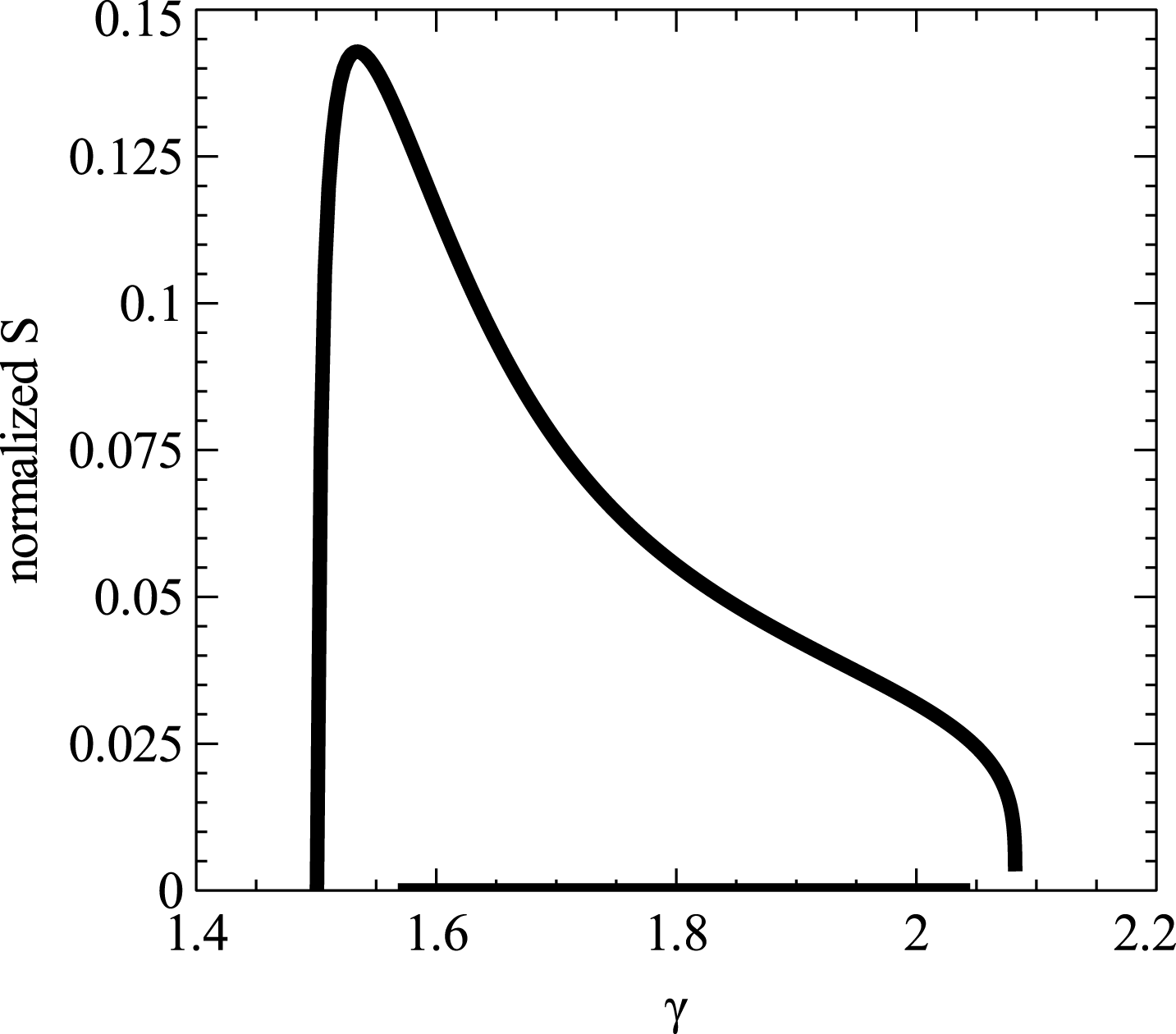
(see scheme in figure 3):
 $$\begin{eqnarray}{\displaystyle \frac{\text{d}S_{\text{sep}}}{\text{d}t}}<0\quad \text{for }\unicode[STIX]{x1D6FE}\in \text{Z}_{\text{esc}},\quad \text{and}\quad {\displaystyle \frac{\text{d}S_{\text{sep}}}{\text{d}t}}>0\quad \text{for }\unicode[STIX]{x1D6FE}\in \text{Z}_{\text{trap}}.\end{eqnarray}$$
Therefore, trapping transports particles toward a position in
 $\text{Z}_{\text{esc}}$
from a position in
 $\text{Z}_{\text{trap}}$
. In this study, we assume that wave intensity maximizes at intermediate
 $z$
and drops to zero at both
 $z=0$
and large
 $z$
. Therefore, trapping into resonance and escape from the resonance occur within the same hemisphere (
 $z>0$
). We do not consider the more complicated situation where waves with trapped particles can cross the
 $z=0$
plane several times. Therefore, particle transport in energy space is limited by the time scale of trapped particle motion in the resonance (approximately a quarter of particle bounce period). This transport is described by the map
 $\unicode[STIX]{x1D6FE}=Y(\unicode[STIX]{x1D6FE}^{\ast })$
where
 $\unicode[STIX]{x1D6FE}\in \text{Z}_{\text{esc}}$
and
 $\unicode[STIX]{x1D6FE}^{\ast }\in \text{Z}_{\text{trap}}$
. The function
 $Y(\unicode[STIX]{x1D6FE}^{\ast })$
is defined by equation
 $S_{\text{sep}}(\unicode[STIX]{x1D6FE}^{\ast })=S_{\text{sep}}(\unicode[STIX]{x1D6FE})$
. As shown in Artemyev et al. (Reference Artemyev, Neishtadt, Vasiliev and Mourenas2016), to write the generalized Fokker–Plank equation, we need to determine only the relation
 $\langle \unicode[STIX]{x0394}\unicode[STIX]{x1D6FE}\rangle =\langle \unicode[STIX]{x0394}\unicode[STIX]{x1D6FE}\rangle (\unicode[STIX]{x1D6FE})$
and the map
 $\unicode[STIX]{x1D6FE}=Y(\unicode[STIX]{x1D6FE}^{\ast })$
.
Normalized area
 $S_{\text{sep}}(\unicode[STIX]{x1D6FE})$
given by (2.27).

3 Generalized Fokker–Planck equation
Resonant wave–particle interactions lead to particle scattering, which can be defined via two physical quantities: a diffusion coefficient
 $D_{\unicode[STIX]{x1D6FE}\unicode[STIX]{x1D6FE}}=\langle (\unicode[STIX]{x0394}\unicode[STIX]{x1D6FE})^{2}\rangle /2T(\unicode[STIX]{x1D6FE})$
and a drift velocity
 $V_{\unicode[STIX]{x1D6FE}}=\langle \unicode[STIX]{x0394}\unicode[STIX]{x1D6FE}\rangle /T(\unicode[STIX]{x1D6FE})$
. (Note, we consider unidirectional wave propagation, and thus there is a finite
 $\unicode[STIX]{x0394}\unicode[STIX]{x1D6FE}$
.) These two characteristics describe respectively particle diffusion and particle drift in
 $\unicode[STIX]{x1D6FE}$
space (for fixed
 $\tilde{I} _{x}=\text{const.}$
). The corresponding evolution of the particle distribution function can be written in terms of two operators
 $$\begin{eqnarray}\displaystyle \left.\begin{array}{@{}c@{}}\hat{L}_{D}\unicode[STIX]{x1D6F9}={\displaystyle \frac{\unicode[STIX]{x2202}}{\unicode[STIX]{x2202}\unicode[STIX]{x1D6FE}}}\left(D_{\unicode[STIX]{x1D6FE}\unicode[STIX]{x1D6FE}}{\displaystyle \frac{\unicode[STIX]{x2202}\unicode[STIX]{x1D6F9}}{\unicode[STIX]{x2202}\unicode[STIX]{x1D6FE}}}\right)\\ \hat{L}_{V}\unicode[STIX]{x1D6F9}=-{\displaystyle \frac{\unicode[STIX]{x2202}V_{\unicode[STIX]{x1D6FE}}\unicode[STIX]{x1D6F9}}{\unicode[STIX]{x2202}\unicode[STIX]{x1D6FE}}}.\end{array}\right\} & & \displaystyle\end{eqnarray}$$
The third effect is particle trapping and fast transport. This effect can be described by probabilistic operators (Solovev & Shklyar Reference Solovev and Shklyar1986; Artemyev et al.
Reference Artemyev, Vasiliev, Mourenas, Agapitov, Krasnoselskikh, Boscher and Rolland2014; Omura et al.
Reference Omura, Miyashita, Yoshikawa, Summers, Hikishima, Ebihara and Kubota2015). This kind of operator depends on the probability of trapping
 $\unicode[STIX]{x1D6F1}=-\text{d}\langle \unicode[STIX]{x0394}I\rangle /\text{d}I$
(Artemyev et al.
Reference Artemyev, Neishtadt, Vasiliev and Mourenas2016, Reference Artemyev, Neishtadt, Vasiliev and Mourenas2017a
) and can be written as
 $$\begin{eqnarray}\left.\begin{array}{@{}c@{}}\hat{L}_{T}\unicode[STIX]{x1D6F9}=-{\displaystyle \frac{\unicode[STIX]{x1D6F1}}{T}}\unicode[STIX]{x1D6F9}={\displaystyle \frac{\unicode[STIX]{x1D6F9}}{T}}{\displaystyle \frac{\text{d}\langle \unicode[STIX]{x0394}\unicode[STIX]{x1D6FE}\rangle }{\text{d}\unicode[STIX]{x1D6FE}}},\quad \unicode[STIX]{x1D6FE}\in \text{Z}_{\text{trap}}\\ \hat{L}_{T}\unicode[STIX]{x1D6F9}=-{\displaystyle \frac{\unicode[STIX]{x1D6F1}^{\ast }}{T^{\ast }}}\unicode[STIX]{x1D6F9}^{\ast }\left|{\displaystyle \frac{\text{d}\unicode[STIX]{x1D6FE}^{\ast }}{\text{d}\unicode[STIX]{x1D6FE}}}\right|={\displaystyle \frac{\unicode[STIX]{x1D6F9}^{\ast }}{T^{\ast }}}{\displaystyle \frac{\text{d}\langle \unicode[STIX]{x0394}\unicode[STIX]{x1D6FE}\rangle }{\text{d}\unicode[STIX]{x1D6FE}}},\quad \unicode[STIX]{x1D6FE}\in \text{Z}_{\text{esc}},\end{array}\right\}\end{eqnarray}$$
where
 $\unicode[STIX]{x1D6F1}^{\ast }=\unicode[STIX]{x1D6F1}(\unicode[STIX]{x1D6FE}^{\ast })$
,
 $\unicode[STIX]{x1D6F9}^{\ast }=\unicode[STIX]{x1D6F9}(\unicode[STIX]{x1D6FE})$
and
 $\unicode[STIX]{x1D6FE}^{\ast }$
is a solution of equation
 $\unicode[STIX]{x1D6FE}=Y(\unicode[STIX]{x1D6FE}^{\ast })$
. Note that in (3.2) we use the linear relation between
 $I$
and
 $\unicode[STIX]{x1D6FE}$
. Combining equations (3.1) and (3.2), and using
 $\langle \unicode[STIX]{x0394}\unicode[STIX]{x1D6FE}\rangle =T(\unicode[STIX]{x1D6FE})V_{\unicode[STIX]{x1D6FE}}$
, we obtain the final form of the equation for
 $\unicode[STIX]{x1D6F9}$
(
 $\unicode[STIX]{x2202}\unicode[STIX]{x1D6F9}/\unicode[STIX]{x2202}t=\hat{L}_{D}\unicode[STIX]{x1D6F9}+\hat{L}_{V}\unicode[STIX]{x1D6F9}+\hat{L}_{T}\unicode[STIX]{x1D6F9}$
):
 $$\begin{eqnarray}\displaystyle \left.\begin{array}{@{}rcl@{}}{\displaystyle \frac{\unicode[STIX]{x2202}\unicode[STIX]{x1D6F9}}{\unicode[STIX]{x2202}t}}\, & =\, & -V_{\unicode[STIX]{x1D6FE}}{\displaystyle \frac{\unicode[STIX]{x2202}\unicode[STIX]{x1D6F9}}{\unicode[STIX]{x2202}\unicode[STIX]{x1D6FE}}}+{\displaystyle \frac{1}{T}}{\displaystyle \frac{\text{d}T}{\text{d}\unicode[STIX]{x1D6FE}}}V\unicode[STIX]{x1D6F9}+{\displaystyle \frac{\unicode[STIX]{x2202}}{\unicode[STIX]{x2202}\unicode[STIX]{x1D6FE}}}\left(D_{\unicode[STIX]{x1D6FE}\unicode[STIX]{x1D6FE}}{\displaystyle \frac{\unicode[STIX]{x2202}\unicode[STIX]{x1D6F9}}{\unicode[STIX]{x2202}\unicode[STIX]{x1D6FE}}}\right),\quad \unicode[STIX]{x1D6FE}\in \text{Z}_{\text{trap}}\\ {\displaystyle \frac{\unicode[STIX]{x2202}\unicode[STIX]{x1D6F9}}{\unicode[STIX]{x2202}t}}\, & =\, & -V_{\unicode[STIX]{x1D6FE}}{\displaystyle \frac{\unicode[STIX]{x2202}\unicode[STIX]{x1D6F9}}{\unicode[STIX]{x2202}\unicode[STIX]{x1D6FE}}}-{\displaystyle \frac{\unicode[STIX]{x2202}V_{\unicode[STIX]{x1D6FE}}}{\unicode[STIX]{x2202}\unicode[STIX]{x1D6FE}}}\left(\unicode[STIX]{x1D6F9}-{\displaystyle \frac{T}{T^{\ast }}}\unicode[STIX]{x1D6F9}^{\ast }\right)+{\displaystyle \frac{1}{T^{\ast }}}{\displaystyle \frac{\text{d}T^{\ast }}{\text{d}\unicode[STIX]{x1D6FE}}}V_{\unicode[STIX]{x1D6FE}}\unicode[STIX]{x1D6F9}^{\ast }\\ \, & \, & +\,{\displaystyle \frac{\unicode[STIX]{x2202}}{\unicode[STIX]{x2202}\unicode[STIX]{x1D6FE}}}\left(D_{\unicode[STIX]{x1D6FE}\unicode[STIX]{x1D6FE}}{\displaystyle \frac{\unicode[STIX]{x2202}\unicode[STIX]{x1D6F9}}{\unicode[STIX]{x2202}\unicode[STIX]{x1D6FE}}}\right),\quad \unicode[STIX]{x1D6FE}\in \text{Z}_{\text{esc}}.\end{array}\right\} & & \displaystyle\end{eqnarray}$$
We introduce the action of the averaged system
 $J$
as
 $\text{d}J/\text{d}\unicode[STIX]{x1D6FE}=T(\unicode[STIX]{x1D6FE})/2\unicode[STIX]{x03C0}$
and rewrite (3.3) for
 $J$
using the function
 $\unicode[STIX]{x1D6F9}_{J}=2\unicode[STIX]{x03C0}\unicode[STIX]{x1D6F9}/T$
,
 $V_{J}=V_{\unicode[STIX]{x1D6FE}}T/2\unicode[STIX]{x03C0}$
,
 $D_{JJ}=D_{\unicode[STIX]{x1D6FE}\unicode[STIX]{x1D6FE}}T^{2}/4\unicode[STIX]{x03C0}^{2}$
(Artemyev et al.
Reference Artemyev, Neishtadt, Vasiliev and Mourenas2017a
):
 $$\begin{eqnarray}{\displaystyle \frac{\unicode[STIX]{x2202}\unicode[STIX]{x1D6F9}_{J}}{\unicode[STIX]{x2202}t}}=-V_{J}{\displaystyle \frac{\unicode[STIX]{x2202}\unicode[STIX]{x1D6F9}_{J}}{\unicode[STIX]{x2202}J}}+{\displaystyle \frac{\unicode[STIX]{x2202}}{\unicode[STIX]{x2202}J}}\left(D_{JJ}{\displaystyle \frac{\unicode[STIX]{x2202}\unicode[STIX]{x1D6F9}_{\text{J }}}{\unicode[STIX]{x2202}J}}\right)-{\displaystyle \frac{\unicode[STIX]{x2202}V_{J}}{\unicode[STIX]{x2202}J}}\left(\unicode[STIX]{x1D6F9}_{J}-\unicode[STIX]{x1D6F9}_{J}^{\ast }\right)\unicode[STIX]{x1D6E9}+{\displaystyle \frac{\unicode[STIX]{x2202}}{\unicode[STIX]{x2202}J}}(\unicode[STIX]{x1D6FF}V_{J}\unicode[STIX]{x1D6F9}_{J})+C_{J},\end{eqnarray}$$
where
 $\unicode[STIX]{x1D6FF}V_{J}=D_{JJ}\unicode[STIX]{x2202}\ln T/\unicode[STIX]{x2202}J$
, the function
 $\unicode[STIX]{x1D6E9}$
is equal to one when
 $\unicode[STIX]{x1D6FE}\in \text{Z}_{\text{esc}}$
(or
 $\text{d}V_{J}/\text{d}J>0$
) and
 $\unicode[STIX]{x1D6E9}$
is zero when
 $\unicode[STIX]{x1D6FE}\in \text{Z}_{\text{trap}}$
(or
 $\text{d}V_{J}/\text{d}J<0$
); see (2.29)). An additive factor
 $C_{J}$
includes small terms proportional to
 ${\sim}\unicode[STIX]{x2202}\ln T/\unicode[STIX]{x2202}J$
and we omit this factor for further calculations. There are two drift terms in (3.4):
 ${\sim}V_{J}$
and
 ${\sim}\unicode[STIX]{x1D6FF}V_{J}\sim D_{JJ}$
. Equation (2.26) shows that
 $V_{J}\sim \unicode[STIX]{x0394}\unicode[STIX]{x1D6FE}\sim \sqrt{eA_{0}/m_{e}c^{2}}$
, whereas
 $\unicode[STIX]{x1D6FF}V_{J}\sim (\unicode[STIX]{x0394}\unicode[STIX]{x1D6FE})^{2}\sim eA_{0}/m_{e}c^{2}\ll V_{J}$
. Thus, we keep only one drift term
 ${\sim}V_{J}$
in (3.4). Moreover, we should note that to write (3.1), we omit terms smaller than
 ${\sim}O(eA_{0}/m_{e}c)$
. Equation (3.4) describes the evolution of the
 $\unicode[STIX]{x1D6F9}_{J}(J)$
distribution, which can be transformed back to the
 $\unicode[STIX]{x1D6F9}(\unicode[STIX]{x1D6FE})$
distribution using
 $\text{d}J/\text{d}\unicode[STIX]{x1D6FE}=T(\unicode[STIX]{x1D6FE})/2\unicode[STIX]{x03C0}$
. This evolution includes many resonant interactions (many trappings and scatterings), but each interaction is localized in time (trapping lasts for a time interval smaller than the bounce period). Thus, equation (3.4) describes the long-term evolution of the particle distribution function averaged over a bounce period.
4 Parallel propagating waves: cyclotron resonance
In this section, we consider nonlinear resonant electron interaction with parallel propagating whistler mode waves (i.e. with
 $k_{x}=0$
and
 $C_{1}=C_{2}=C=1$
in (2.13)). Therefore,
 $n=-1$
and the Hamiltonian
 $H_{1}$
takes the form
 $$\begin{eqnarray}H_{1}=-eA_{0}{\displaystyle \frac{\unicode[STIX]{x1D70C}\unicode[STIX]{x1D6FA}_{0}}{c\unicode[STIX]{x1D6FE}}}\sin (\unicode[STIX]{x1D719}_{\Vert }+\unicode[STIX]{x1D713}-\unicode[STIX]{x03C0}/2)\end{eqnarray}$$
and there are no other resonances (the corresponding Bessel functions in (2.13) are equal to zero). We consider a magnetic field model with
 $\unicode[STIX]{x1D6FA}_{0}(s/R)$
, where
 $R$
is the spatial scale of the field gradient. We also use the dipole magnetic latitude
 $\unicode[STIX]{x1D706}$
instead of
 $s$
:
 $\text{d}s/\text{d}\unicode[STIX]{x1D706}=R\sqrt{1+3\sin ^{2}\unicode[STIX]{x1D706}}\cos \unicode[STIX]{x1D706}$
and
 $\unicode[STIX]{x1D6FA}_{0}=\unicode[STIX]{x1D6FA}_{0}(0)\sqrt{1+3\sin ^{2}\unicode[STIX]{x1D706}}/\cos ^{6}\unicode[STIX]{x1D706}$
. Introducing the dimensionless frequency
 $\unicode[STIX]{x1D71B}=\unicode[STIX]{x1D714}_{-1}=\unicode[STIX]{x1D6FA}_{0}(s)/\unicode[STIX]{x1D714}$
and using the simplified dispersion relation valid for parallel propagating waves (Stix Reference Stix1962), we write:
 $$\begin{eqnarray}N_{\Vert }={\displaystyle \frac{\unicode[STIX]{x1D6FA}_{\text{pe}}}{\unicode[STIX]{x1D714}}}(\unicode[STIX]{x1D71B}-1)^{-1/2},\quad {\displaystyle \frac{\unicode[STIX]{x2202}\ln N_{\Vert }}{\unicode[STIX]{x2202}\ln \unicode[STIX]{x1D6FA}_{0}}}=-{\displaystyle \frac{1}{2}}\unicode[STIX]{x1D71B}(\unicode[STIX]{x1D71B}-1)^{-1},\end{eqnarray}$$
where
 $\unicode[STIX]{x1D6FA}_{\text{pe}}=\text{const.}$
is the plasma frequency. Note that
 $N_{\Vert }$
is the refractive index
 $N$
of parallel propagating waves. Using
 $\unicode[STIX]{x1D714}_{n}=-n\unicode[STIX]{x1D6FA}_{0}/\unicode[STIX]{x1D714}=\unicode[STIX]{x1D71B}$
, we rewrite
 $\unicode[STIX]{x1D700}=(\unicode[STIX]{x1D6FD}_{\bot }^{2}-2\unicode[STIX]{x1D6FE}_{\text{init}}\unicode[STIX]{x1D714}_{n})$
as:
 $$\begin{eqnarray}\unicode[STIX]{x1D700}=\unicode[STIX]{x1D6FD}_{\bot }^{2}-2\unicode[STIX]{x1D6FE}_{\text{init}}\unicode[STIX]{x1D714}_{n}={\displaystyle \frac{\unicode[STIX]{x1D6FA}_{0}}{\unicode[STIX]{x1D714}}}\left({\displaystyle \frac{2\unicode[STIX]{x1D714}\tilde{I} _{x}}{m_{e}c^{2}}}-2\unicode[STIX]{x1D6FE}_{\text{init}}\right)=\unicode[STIX]{x1D71B}\unicode[STIX]{x1D700}_{0},\end{eqnarray}$$
where
 $\unicode[STIX]{x1D700}_{0}$
is a constant. Equations (4.2), (4.3) allow us to simplify equations (2.24), (2.27), (2.28) as:
 $$\begin{eqnarray}\displaystyle \left.\begin{array}{@{}c@{}}\unicode[STIX]{x1D6FE}=\left|\unicode[STIX]{x1D71B}-{\displaystyle \frac{N_{\Vert }}{\sqrt{N_{\Vert }^{2}-1}}}\sqrt{1+\unicode[STIX]{x1D700}_{0}\unicode[STIX]{x1D71B}+\unicode[STIX]{x1D71B}^{2}}\right|\\ T={\displaystyle \frac{\unicode[STIX]{x1D6FE}}{\sqrt{\unicode[STIX]{x1D6FE}^{2}-1}}}\displaystyle \oint \left(1-{\displaystyle \frac{\unicode[STIX]{x1D700}_{0}+2\unicode[STIX]{x1D6FE}}{\unicode[STIX]{x1D6FE}^{2}-1}}\unicode[STIX]{x1D71B}(s)\right)^{-1/2}{\displaystyle \frac{\text{d}s}{c}}\\ \bar{r}={\displaystyle \frac{1}{2}}{\displaystyle \frac{N_{\Vert }}{N_{\Vert }^{2}-1}}\left({\displaystyle \frac{\unicode[STIX]{x2202}\ln \unicode[STIX]{x1D6FA}_{0}}{\unicode[STIX]{x2202}s/R}}\right)\left(1-\unicode[STIX]{x1D6FE}^{2}+{\displaystyle \frac{\unicode[STIX]{x1D6FE}^{2}}{N_{\Vert }^{2}}}+{\displaystyle \frac{\unicode[STIX]{x1D71B}}{N_{\Vert }^{2}}}{\displaystyle \frac{\left(\unicode[STIX]{x1D6FE}-\unicode[STIX]{x1D71B}\right)^{2}}{\left(1-\unicode[STIX]{x1D71B}\right)}}-{\displaystyle \frac{\unicode[STIX]{x1D71B}^{2}}{N_{\Vert }^{2}}}\right)\\ \left\langle \unicode[STIX]{x0394}\unicode[STIX]{x1D6FE}\right\rangle =\sqrt{{\displaystyle \frac{a\bar{r}}{\unicode[STIX]{x1D702}\left(N_{\Vert }^{2}-1\right)}}}f_{S}(a),\quad a={\displaystyle \frac{2eA_{0}\unicode[STIX]{x1D702}}{m_{e}c^{2}}}{\displaystyle \frac{\sqrt{(\unicode[STIX]{x1D700}_{0}+2\unicode[STIX]{x1D6FE})\unicode[STIX]{x1D71B}}}{\bar{r}}},\end{array}\right\} & & \displaystyle\end{eqnarray}$$
where
 $\unicode[STIX]{x1D702}=\unicode[STIX]{x1D714}R/c$
.
The system (4.1), (4.4) is characterized by the following parameters: scale
 $R$
, plasma density (defining the plasma frequency
 $\unicode[STIX]{x1D6FA}_{\text{pe}}$
), dimensionless wave amplitude
 $2eA_{e}/m_{e}c^{2}$
, wave frequency
 $\unicode[STIX]{x1D714}$
and
 $\unicode[STIX]{x1D700}_{0}$
. For all following calculations, we use the Earth’s dipole model with
 $R=R_{E}L$
(
 $R_{E}\approx 6380$
km is the Earth’s radius), a plasma density model (Sheeley et al.
Reference Sheeley, Moldwin, Rassoul and Anderson2001) valid outside the plasmasphere in the inner magnetosphere providing
 $\unicode[STIX]{x1D6FA}_{\text{pe}}(L)$
, and consider
 $L=4.5$
(the typical region of intense whistler mode chorus wave observations, see, e.g. Li et al.
Reference Li, Bortnik, Thorne and Angelopoulos2011a
; Agapitov et al.
Reference Agapitov, Artemyev, Krasnoselskikh, Khotyaintsev, Mourenas, Breuillard, Balikhin and Rolland2013),
 $\unicode[STIX]{x1D714}=0.35\unicode[STIX]{x1D6FA}_{0}(0)$
, for the chosen parameters
 $\unicode[STIX]{x1D702}\approx 2000$
,
 $2eA_{e}/m_{e}c^{2}=2a_{0}(\unicode[STIX]{x1D706})/\unicode[STIX]{x1D702}$
(the corresponding wave magnetic field amplitude
 ${\sim}500$
pT is typical for intense whistler mode chorus waves, e.g. Santolík et al.
Reference Santolík, Kletzing, Kurth, Hospodarsky and Bounds2014) and function
 $a_{0}=\exp (-(\unicode[STIX]{x1D706}-\unicode[STIX]{x1D706}_{0})^{2}/\unicode[STIX]{x1D6FF}\unicode[STIX]{x1D706}^{2})$
with
 $\unicode[STIX]{x1D706}_{0}=25^{\circ }$
,
 $\unicode[STIX]{x1D6FF}\unicode[STIX]{x1D706}_{0}=12.5^{\circ }$
imitates a distribution of the wave intensity along magnetic field lines (e.g. Agapitov et al.
Reference Agapitov, Artemyev, Krasnoselskikh, Khotyaintsev, Mourenas, Breuillard, Balikhin and Rolland2013). For the above parameters, the main functions
 $N_{\Vert }$
,
 $\unicode[STIX]{x2202}\ln \unicode[STIX]{x1D6FA}_{0}/\unicode[STIX]{x2202}s/R$
and
 $s/R$
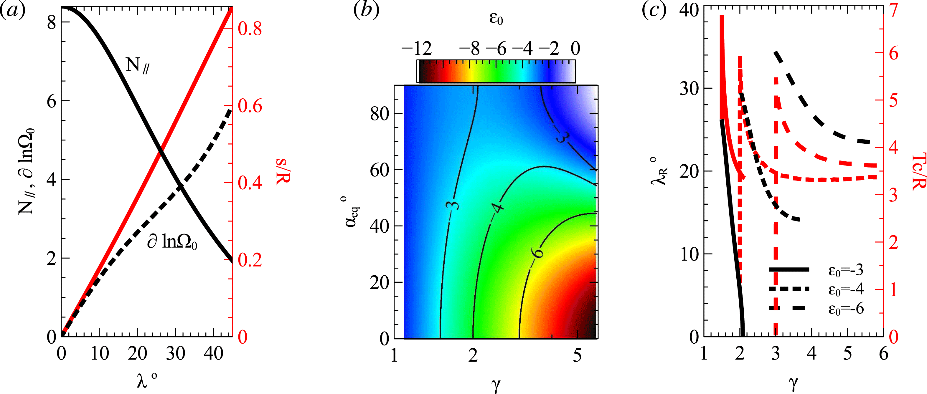
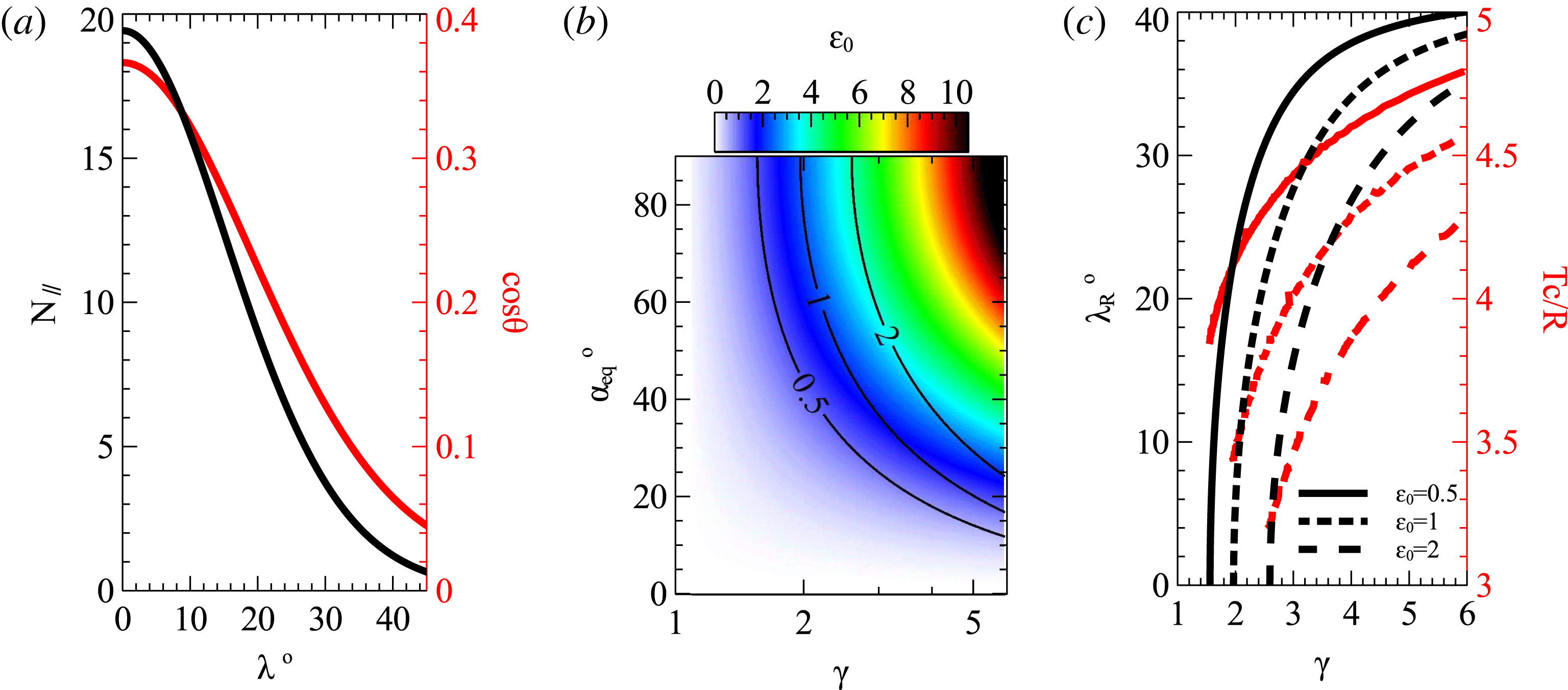
are displayed in figure 4(a) as a function of magnetic latitude
 $\unicode[STIX]{x1D706}$
.
The parameter
 $\unicode[STIX]{x1D700}_{0}$
defines the range of energies and
 $\tilde{I} _{x}$
values considered for a particular solution. It is convenient to introduce the particle pitch angle
 $\unicode[STIX]{x1D6FC}_{\text{eq}}$
(defined at
 $s=0$
) and to rewrite
 $\unicode[STIX]{x1D700}_{0}$
through initial energy and pitch angle. Using the definition of
 $I_{x}$
, we can write
 $2\tilde{I} _{x}=m_{e}c^{2}(\unicode[STIX]{x1D6FE}_{\text{init}}^{2}-1)\sin ^{2}\unicode[STIX]{x1D6FC}_{\text{eq}}$
, and thus
 $\unicode[STIX]{x1D700}_{0}=(\unicode[STIX]{x1D6FE}_{\text{init}}^{2}-1)\sin ^{2}\unicode[STIX]{x1D6FC}_{\text{eq}}/\unicode[STIX]{x1D71B}(0)-2\unicode[STIX]{x1D6FE}_{\text{init}}$
. The function
 $\unicode[STIX]{x1D700}_{0}(\unicode[STIX]{x1D6FE}_{\text{init}},\unicode[STIX]{x1D6FC}_{\text{eq}})=\text{const.}$
corresponds to a certain relation between resonant particle energy and pitch angle, and this relation remains unchanged during the resonant interaction, i.e.
 $\unicode[STIX]{x1D700}_{0}$
can be considered as an integral of particle motion. This integral represents a combination of the particle energy in the wave reference frame and the resonant condition (see analogies of this integral in, e.g. Shklyar Reference Shklyar1981; Summers et al.
Reference Summers, Thorne and Xiao1998). Figure 4(b) shows
 $\unicode[STIX]{x1D700}_{0}(\unicode[STIX]{x1D6FE}_{\text{init}},\unicode[STIX]{x1D6FC}_{\text{eq}})$
. Choosing a particular
 $\unicode[STIX]{x1D700}_{0}$
, we can describe the evolution of a particle ensemble with initial energies and pitch angles defined by
 $\unicode[STIX]{x1D700}_{0}(\unicode[STIX]{x1D6FE}_{\text{init}},\unicode[STIX]{x1D6FC}_{\text{eq}})$
. The definition of the period
 $T$
(see (4.4)) determines the range of energies that must be considered for a given
 $\unicode[STIX]{x1D700}_{0}$
:
 $(2\unicode[STIX]{x1D700}_{0}+2\unicode[STIX]{x1D6FE})\unicode[STIX]{x1D71B}(0)<\unicode[STIX]{x1D6FE}^{2}-1$
. Figure 4(c) shows particle periods
 $T(\unicode[STIX]{x1D6FE})$
and resonant latitudes
 $\unicode[STIX]{x1D706}_{R}$
(defined from the first equation of system (4.4)) for three different
 $\unicode[STIX]{x1D700}_{0}$
values.
(a) Refractive index
 $N_{\Vert }$
, derivative
 $\unicode[STIX]{x2202}\ln \unicode[STIX]{x1D6FA}_{0}/\unicode[STIX]{x2202}s/R$
and field-aligned coordinate
 $s$
are shown as functions of
 $\unicode[STIX]{x1D706}$
. (b) System parameter
 $\unicode[STIX]{x1D700}_{0}$
as a function of initial energy and pitch angle. (c) Periods
 $T(\unicode[STIX]{x1D6FE})$
and resonant latitudes are shown for three values of
 $\unicode[STIX]{x1D700}_{0}$
in the case of parallel whistler mode waves.

To construct (3.4) for the system (4.1), (4.4), we need first to define
 $\langle \unicode[STIX]{x0394}\unicode[STIX]{x1D6FE}\rangle$
,
 $J(\unicode[STIX]{x1D6FE})=\int T(\unicode[STIX]{x1D6FE})\,\text{d}\unicode[STIX]{x1D6FE}/2\unicode[STIX]{x03C0}$
(we use the renormalized
 $Jc/R$
) and
 $J=Y_{J}(J^{\ast })$
projection. Equation (4.4) shows that
 $\langle \unicode[STIX]{x0394}\unicode[STIX]{x1D6FE}\rangle$
depends on
 $\bar{r}(\unicode[STIX]{x1D6FE})$
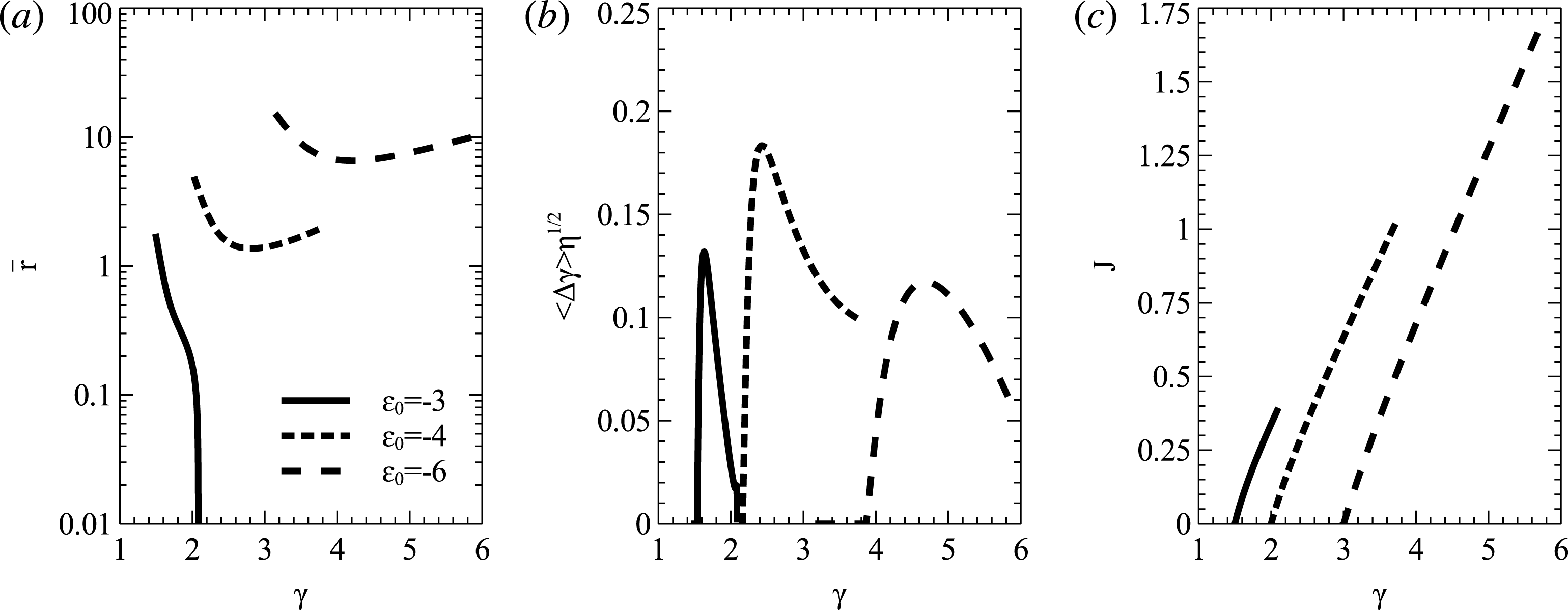
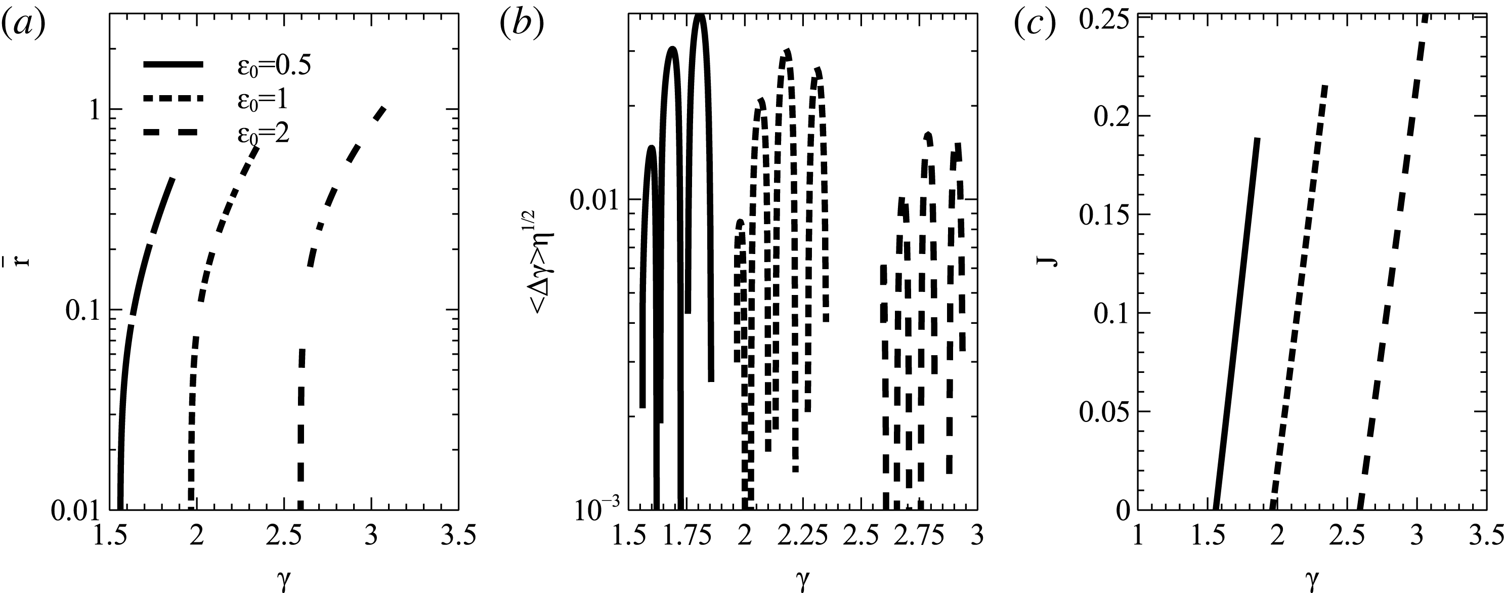
presented in figure 5(a). Using this dependence, we calculate
 $\langle \unicode[STIX]{x0394}\unicode[STIX]{x1D6FE}\rangle$
functions (see figure 5
b) and define
 $V_{\unicode[STIX]{x1D6FE}}=\langle \unicode[STIX]{x0394}\unicode[STIX]{x1D6FE}\rangle /T(\unicode[STIX]{x1D6FE})$
and
 $V_{J}=V_{\unicode[STIX]{x1D6FE}}T/2\unicode[STIX]{x03C0}$
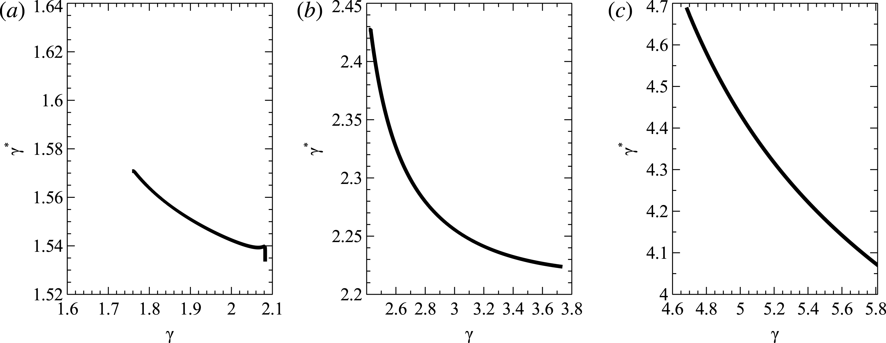
. The non-local (trapping term) of (3.4) is determined by the function
 $\unicode[STIX]{x1D6FE}=Y(\unicode[STIX]{x1D6FE}^{\ast })$
shown in figure 6. A quite limited range of initial
 $\unicode[STIX]{x1D6FE}^{\ast }$
is mapped to a wide range of final
 $\unicode[STIX]{x1D6FE}$
as a result of the nonlinear interaction. The function
 $J(\unicode[STIX]{x1D6FE})$
shown in figure 5(c) allows us to transform the
 $\unicode[STIX]{x1D6FE}$
-dependence into a
 $J$
-dependence and to solve (3.4).
Functions
 $\bar{r}(\unicode[STIX]{x1D6FE})$
(a),
 $\langle \unicode[STIX]{x0394}\unicode[STIX]{x1D6FE}\rangle (\unicode[STIX]{x1D6FE})$
(b),
 $J(\unicode[STIX]{x1D6FE})$
(c) are shown for three values of
 $\unicode[STIX]{x1D700}_{0}$
in the case of parallel whistler mode waves.

The case of parallel whistler mode waves. Dependencies
 $\unicode[STIX]{x1D6FE}=Y(\unicode[STIX]{x1D6FE}^{\ast })$
for three
 $\unicode[STIX]{x1D700}_{0}$
values:
 $\unicode[STIX]{x1D700}_{0}=-3$
(a),
 $\unicode[STIX]{x1D700}_{0}=-4$
(b),
 $\unicode[STIX]{x1D700}_{0}=-6$
(c).

Combining functions
 $J(\unicode[STIX]{x1D6FE})$
,
 $\langle \unicode[STIX]{x0394}\unicode[STIX]{x1D6FE}\rangle$
,
 $\unicode[STIX]{x1D6FE}=Y(\unicode[STIX]{x1D6FE}^{\ast })$
and calculating the diffusion coefficient
 $D_{\unicode[STIX]{x1D6FE}\unicode[STIX]{x1D6FE}}=\langle (\unicode[STIX]{x0394}\unicode[STIX]{x1D6FE})^{2}\rangle /2T(\unicode[STIX]{x1D6FE})$
(see. e.g. Artemyev et al.
Reference Artemyev, Neishtadt, Vasiliev and Mourenas2016; Artemyev et al.
Reference Artemyev, Neishtadt, Vasiliev and Mourenas2017b
), we solve the kinetic equation for the
 $\unicode[STIX]{x1D6F9}_{J}(J)$
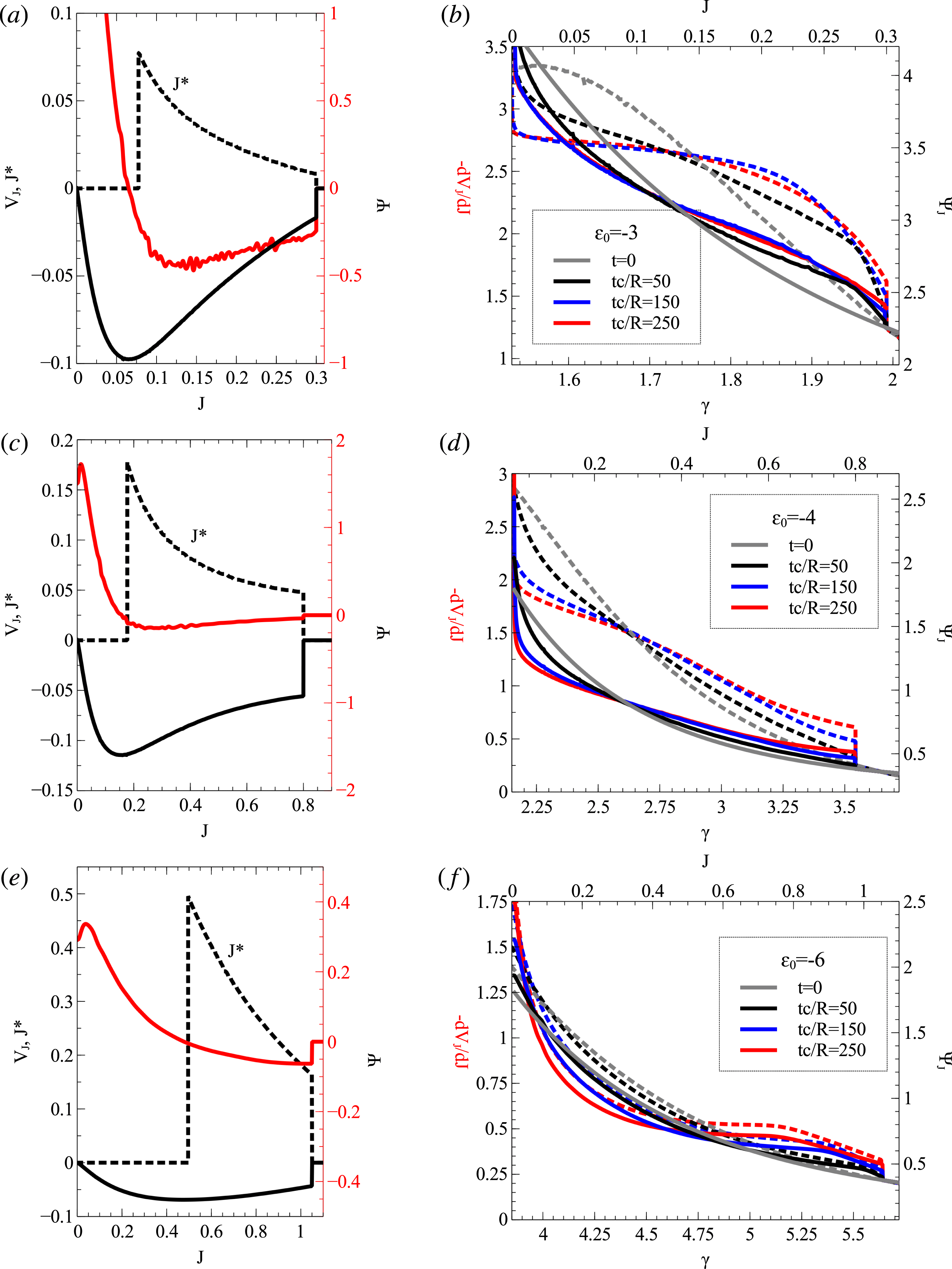
distribution. Figure 7(b,d,f) shows the
 $\unicode[STIX]{x1D6F9}(\unicode[STIX]{x1D6FE})=\unicode[STIX]{x1D6F9}_{J}(J)T/2\unicode[STIX]{x03C0}$
distributions obtained for three different
 $\unicode[STIX]{x1D700}_{0}$
values (the initial distribution
 $\unicode[STIX]{x1D6F9}(\unicode[STIX]{x1D6FE})\sim \unicode[STIX]{x1D6FE}^{-5}$
is shown by grey colour). Each
 $\unicode[STIX]{x1D700}_{0}$
corresponds to some range of
 $\unicode[STIX]{x1D6FE}$
,
 $\unicode[STIX]{x1D6FC}_{\text{eq}}$
(see figure 4
b), and for different
 $\unicode[STIX]{x1D700}_{0}$
the evolution of
 $\unicode[STIX]{x1D6F9}(\unicode[STIX]{x1D6FE})$
reflects the dominance of particle trapping (
 $\unicode[STIX]{x1D6FE}$
increase) or drift (
 $\unicode[STIX]{x1D6FE}$
decrease). We use boundary conditions
 $\unicode[STIX]{x2202}\unicode[STIX]{x1D6F9}/\unicode[STIX]{x2202}J=0$
at the right-hand side (large
 $J$
; large
 $\unicode[STIX]{x1D6FE}$
) and left-hand side (small
 $J$
; small
 $\unicode[STIX]{x1D6FE}$
) boundaries. This condition allows a variation of boundary
 $\unicode[STIX]{x1D6F9}$
values, but guarantees the absence of particle flux outside the
 $J$
range of the simulation. For all
 $\unicode[STIX]{x1D700}_{0}$
, the nonlinear wave–particle interaction results in the generation of a high-energy population due to trapping, which transports particles to higher
 $\unicode[STIX]{x1D6FE}$
. This population gradually drifts toward smaller energies, but this drift is weaker than the effect of trapping, i.e. the phase space density of high-energy particles grows. In all three cases, the distribution evolves toward a more uniform profile
 $\unicode[STIX]{x1D6F9}(J)$
and we expect that after a sufficiently long time interval the final distribution will be
 $\unicode[STIX]{x1D6F9}(J)\approx \text{const.}$
, i.e.
 $\unicode[STIX]{x1D6F9}$
will evolve toward the stationary solution of (3.4). The evolution of the entire particle distribution consists in
 $\unicode[STIX]{x1D6F9}(\unicode[STIX]{x1D6FE})$
evolutions for a wide range of
 $\unicode[STIX]{x1D700}_{0}$
values and, as a result, particle acceleration can be compensated by the deceleration of other particles, in such a way that the total energy variation of the entire particle ensemble can remain small (Shklyar Reference Shklyar2011, Reference Shklyar2017).
The case of parallel whistler mode waves. (a,c,e) Show the distributions of
 $\unicode[STIX]{x1D702}^{-1/2}V_{J}(J)$
,
 $-\unicode[STIX]{x1D702}^{-1/2}\,\text{d}V_{J}/\text{d}J$
, and
 $J^{\ast }(J)$
(inverse
 $Y_{J}(J^{\ast })$
function). (b,d,f) Show the distributions
 $\unicode[STIX]{x1D6F9}_{J}(J)$
(dashed) and
 $\unicode[STIX]{x1D6F9}(\unicode[STIX]{x1D6FE})$
(solid) at three different times
 $tc/R$
. The data are plotted for three different
 $\unicode[STIX]{x1D700}_{0}$
values.

5 Strongly oblique waves: Landau resonance
In this section, we consider electrons in Landau resonance
 $n=0$
with strongly oblique whistler mode waves propagating with
 $\unicode[STIX]{x1D703}$
within one degree from the resonant cone angle
 $\unicode[STIX]{x1D703}_{r}=\arccos (\unicode[STIX]{x1D714}/\unicode[STIX]{x1D6FA}_{0})$
(Stix Reference Stix1962). Therefore, the Hamiltonian
 $H_{1}$
from (2.13) takes the form
 $$\begin{eqnarray}\left.\begin{array}{@{}c@{}}H_{1}=-eA_{0}h^{(0)}\sin \unicode[STIX]{x1D719}_{\Vert }\\ h^{(0)}=-{\displaystyle \frac{\unicode[STIX]{x1D70C}\unicode[STIX]{x1D6FA}_{0}}{c\unicode[STIX]{x1D6FE}}}CJ_{1}(k_{x}\unicode[STIX]{x1D70C})-\left({\displaystyle \frac{p_{z}}{\unicode[STIX]{x1D6FE}m_{e}c}}+C_{3}\right)\sin \unicode[STIX]{x1D703}J_{0}(k_{x}\unicode[STIX]{x1D70C}),\end{array}\right\}\end{eqnarray}$$
where
 $p_{z}=k_{z}I_{R}+p_{R}=\unicode[STIX]{x1D6FE}/N_{\Vert }$
. As in the previous section, we consider a magnetic field model with
 $\unicode[STIX]{x1D6FA}=\unicode[STIX]{x1D6FA}(0)\sqrt{1+3\sin ^{2}\unicode[STIX]{x1D706}}/\cos ^{6}\unicode[STIX]{x1D706}$
and
 $\text{d}s/\text{d}\unicode[STIX]{x1D706}=R\sqrt{1+3\sin ^{2}\unicode[STIX]{x1D706}}\cos \unicode[STIX]{x1D706}$
, where
 $R$
is the spatial scale of magnetic field inhomogeneity. Using
 $\unicode[STIX]{x1D71B}=\unicode[STIX]{x1D6FA}_{0}(s)/\unicode[STIX]{x1D714}$
and a simplified dispersion relation valid for obliquely propagating waves (Stix Reference Stix1962), we write:
 $$\begin{eqnarray}N_{\Vert }={\displaystyle \frac{\unicode[STIX]{x1D6FA}_{\text{pe}}\cos \unicode[STIX]{x1D703}}{\unicode[STIX]{x1D714}\sqrt{\unicode[STIX]{x1D71B}\cos \unicode[STIX]{x1D703}-1}}},\quad {\displaystyle \frac{\unicode[STIX]{x2202}\ln N_{\Vert }}{\unicode[STIX]{x2202}\ln \unicode[STIX]{x1D6FA}_{0}}}=-{\displaystyle \frac{1}{2}}{\displaystyle \frac{\unicode[STIX]{x1D71B}\cos \unicode[STIX]{x1D703}}{\unicode[STIX]{x1D71B}\cos \unicode[STIX]{x1D703}-1}},\end{eqnarray}$$
where
 $\unicode[STIX]{x1D6FA}_{\text{pe}}=\text{const.}$
is the plasma frequency. Using
 $\unicode[STIX]{x1D714}_{n}=0$
, we rewrite
 $\unicode[STIX]{x1D700}=\unicode[STIX]{x1D6FD}_{\bot }^{2}-2\unicode[STIX]{x1D6FE}_{\text{init}}\unicode[STIX]{x1D714}_{n}$
as:
 $$\begin{eqnarray}\unicode[STIX]{x1D700}=\unicode[STIX]{x1D6FD}_{\bot }^{2}={\displaystyle \frac{\unicode[STIX]{x1D6FA}_{0}}{\unicode[STIX]{x1D714}}}{\displaystyle \frac{2\unicode[STIX]{x1D714}\tilde{I} _{x}}{m_{e}c^{2}}}=\unicode[STIX]{x1D71B}\unicode[STIX]{x1D700}_{0},\end{eqnarray}$$
where
 $\unicode[STIX]{x1D700}_{0}$
is a constant. Equations (5.2), (5.3) allow us to simplify (2.24), (2.25), (2.28):
 $$\begin{eqnarray}\displaystyle \hspace{-12.0pt}\left.\begin{array}{@{}c@{}}\unicode[STIX]{x1D6FE}={\displaystyle \frac{N_{\Vert }}{\sqrt{N_{\Vert }^{2}-1}}}\sqrt{1+\unicode[STIX]{x1D700}_{0}\unicode[STIX]{x1D71B}},\quad T={\displaystyle \frac{\unicode[STIX]{x1D6FE}}{\sqrt{\unicode[STIX]{x1D6FE}^{2}-1}}}\displaystyle \oint \left(1-{\displaystyle \frac{\unicode[STIX]{x1D700}_{0}\unicode[STIX]{x1D71B}(s)}{\unicode[STIX]{x1D6FE}^{2}-1}}\right)^{-1/2}{\displaystyle \frac{\text{d}s}{c}}\\ \bar{r}={\displaystyle \frac{1}{2}}{\displaystyle \frac{N_{\Vert }}{N_{\Vert }^{2}-1}}\left({\displaystyle \frac{\unicode[STIX]{x2202}\ln \unicode[STIX]{x1D6FA}_{0}}{\unicode[STIX]{x2202}s/R}}\right)\left(1-\unicode[STIX]{x1D6FE}^{2}-{\displaystyle \frac{\unicode[STIX]{x1D6FE}^{2}}{N_{\Vert }^{2}}}{\displaystyle \frac{1}{\unicode[STIX]{x1D71B}\cos \unicode[STIX]{x1D703}-1}}\right)\\ \langle \unicode[STIX]{x0394}\unicode[STIX]{x1D6FE}\rangle =\sqrt{{\displaystyle \frac{a\bar{r}}{\unicode[STIX]{x1D702}\left(N_{\Vert }^{2}-1\right)}}}f_{S}(a),\quad a={\displaystyle \frac{2eA_{0}\unicode[STIX]{x1D702}}{m_{e}c^{2}}}{\displaystyle \frac{\sqrt{\unicode[STIX]{x1D700}_{0}\unicode[STIX]{x1D71B}}h^{(0)}}{\bar{r}}},\quad k_{x}\unicode[STIX]{x1D70C}=\sqrt{\unicode[STIX]{x1D700}_{0}\unicode[STIX]{x1D71B}}{\displaystyle \frac{N_{\Vert }}{\unicode[STIX]{x1D71B}}}{\displaystyle \frac{\sin \unicode[STIX]{x1D703}}{\cos \unicode[STIX]{x1D703}}}\\ h^{(0)}=-{\displaystyle \frac{\sqrt{\unicode[STIX]{x1D700}_{0}\unicode[STIX]{x1D71B}}}{\unicode[STIX]{x1D6FE}}}CJ_{1}(k_{x}\unicode[STIX]{x1D70C})-(N_{\Vert }+C_{3})\sin \unicode[STIX]{x1D703}J_{0}(k_{x}\unicode[STIX]{x1D70C}),\end{array}\right\} & & \displaystyle\end{eqnarray}$$
where
 $\unicode[STIX]{x1D702}=\unicode[STIX]{x1D714}R/c$
. Similarly to (4.1), (4.4), equations (5.4) include several parameters: we use the same scale
 $R$
,
 $\unicode[STIX]{x1D714}$
and plasma density
 $\unicode[STIX]{x1D6FA}_{\text{pe}}$
as for parallel propagating wave (and, thus
 $\unicode[STIX]{x1D702}\approx 2000$
), whereas the dimensionless wave amplitude is taken as
 $2eA_{e}/m_{e}c^{2}=1.5a_{0}(\unicode[STIX]{x1D706})/\unicode[STIX]{x1D702}$
(the corresponding wave magnetic field amplitude
 ${\sim}150$
pT is typical of intense highly oblique whistler mode chorus waves, e.g. Cully et al.
Reference Cully, Bonnell and Ergun2008; Wilson et al.
Reference Wilson, Cattell, Kellogg, Wygant, Goetz, Breneman and Kersten2011; Agapitov et al.
Reference Agapitov, Artemyev, Mourenas, Krasnoselskikh, Bonnell, Le Contel, Cully and Angelopoulos2014). Figure 8(a) shows the parallel refractive index
 $N_{\Vert }$
and
 $\cos \unicode[STIX]{x1D703}$
along the magnetic latitude
 $\unicode[STIX]{x1D706}$
. As latitude increases,
 $\unicode[STIX]{x1D703}$
increases too, whereas
 $\cos \unicode[STIX]{x1D703}$
decreases to zero.
Equation (5.3) shows that the parameter
 $\unicode[STIX]{x1D700}_{0}=(\unicode[STIX]{x1D6FE}_{\text{init}}^{2}-1)\sin ^{2}\unicode[STIX]{x1D6FC}_{\text{eq}}/\unicode[STIX]{x1D71B}(0)$
is positive and equal to the initial
 $I_{x}/\unicode[STIX]{x1D71B}(0)$
value (i.e. for Landau resonance the
 $\unicode[STIX]{x1D700}_{0}$
conservation means the conservation of the magnetic moment
 $I_{x}$
). For Landau resonance
 $n=0$
, the wave phase does not depend on the phase conjugated to
 $I_{x}$
, and thus
 $I_{x}$
is conserved for all particles (see Hamiltonian (2.14)). It is convenient to introduce the particle pitch angle
 $\unicode[STIX]{x1D6FC}_{\text{eq}}$
(defined at
 $s=0$
) and to rewrite
 $\unicode[STIX]{x1D700}_{0}$
as a function of initial energy and pitch angle. Figure 8(b) shows
 $\unicode[STIX]{x1D700}_{0}(\unicode[STIX]{x1D6FE}_{\text{init}},\unicode[STIX]{x1D6FC}_{\text{eq}})$
. For calculations within this section, we use three
 $\unicode[STIX]{x1D700}$
values:
 $0.5$
,
 $1$
and
 $2$
. Using these
 $\unicode[STIX]{x1D700}_{0}$
, we plot in figure 4(c) the particle periods
 $T(\unicode[STIX]{x1D6FE})$
and resonant latitudes
 $\unicode[STIX]{x1D706}_{R}$
(defined from the first equation of system (5.4)).
The case of very oblique whistler mode waves. (a) Refractive index
 $N_{\Vert }$
and
 $\cos \unicode[STIX]{x1D703}$
are shown as functions of
 $\unicode[STIX]{x1D706}$
. (b) System parameter
 $\unicode[STIX]{x1D700}_{0}$
as a function of initial energy and pitch angle. (c) Periods
 $T(\unicode[STIX]{x1D6FE})$
and resonant latitudes for three values of
 $\unicode[STIX]{x1D700}_{0}$
.

Using (5.4), we define the functions
 $\bar{r}(\unicode[STIX]{x1D6FE})$
and
 $J(\unicode[STIX]{x1D6FE})=\int T\,\text{d}\unicode[STIX]{x1D6FE}/2\unicode[STIX]{x03C0}$
(we use the renormalized
 $J=Jc/R$
) and plot them in figure 9. These functions have similar profiles as in the case of cyclotron resonance with parallel propagating waves (see figure 5). Unlike
 $\bar{r}(\unicode[STIX]{x1D6FE})$
,
 $J(\unicode[STIX]{x1D6FE})$
, however, the function
 $\langle \unicode[STIX]{x0394}\unicode[STIX]{x1D6FE}\rangle$
has a much more complicated profile for Landau resonance (compare the central panels of figures 5 and 9). The effective wave amplitude given by (5.4) depends on a combination of Bessel functions
 $J_{0}$
,
 $J_{1}$
, and thus this amplitude oscillates along the resonant particle trajectory (with
 $\unicode[STIX]{x1D6FE}$
). Such oscillations result in several maxima/minima of
 $\langle \unicode[STIX]{x0394}\unicode[STIX]{x1D6FE}\rangle$
, i.e. the particles can get trapped in many regions (with trapping condition
 $\text{d}S_{\text{sep}}/\text{d}\unicode[STIX]{x1D6FE}=\text{d}\langle \unicode[STIX]{x0394}\unicode[STIX]{x1D6FE}\rangle /\text{d}\unicode[STIX]{x1D6FE}>0$
, see (2.29a,b
)) separated in
 $\unicode[STIX]{x1D6FE}$
space by regions where particle escape from trapping (where
 $\text{d}S_{\text{sep}}/\text{d}\unicode[STIX]{x1D6FE}=\,\text{d}\langle \unicode[STIX]{x0394}\unicode[STIX]{x1D6FE}\rangle /\text{d}\unicode[STIX]{x1D6FE}<0$
).
Figure 10 demonstrates that the
 $Y(\unicode[STIX]{x1D6FE}^{\ast })$
function contains several regions with very sharp gradients (several almost vertical lines). Thus, all particles trapped within a wide energy
 $\unicode[STIX]{x1D6FE}^{\ast }$
range (within a region with
 $\text{d}\langle \unicode[STIX]{x0394}\unicode[STIX]{x1D6FE}\rangle /\text{d}\unicode[STIX]{x1D6FE}>0$
) will escape at the next (after the trapping region) decrease of
 $\langle \unicode[STIX]{x0394}\unicode[STIX]{x1D6FE}\rangle$
with almost the same energy
 $\unicode[STIX]{x1D6FE}=Y(\unicode[STIX]{x1D6FE}^{\ast })$
. Using the functions shown in figures 9 and 10, we can calculate all coefficients of (3.4).
Functions
 $\bar{r}(\unicode[STIX]{x1D6FE})$
(a),
 $\langle \unicode[STIX]{x0394}\unicode[STIX]{x1D6FE}\rangle (\unicode[STIX]{x1D6FE})$
(b),
 $J(\unicode[STIX]{x1D6FE})$
(c) for three different values of
 $\unicode[STIX]{x1D700}_{0}$
in the case of very oblique whistler mode waves.

Dependencies
 $\unicode[STIX]{x1D6FE}=Y(\unicode[STIX]{x1D6FE}^{\ast })$
for three
 $\unicode[STIX]{x1D700}_{0}$
values in the case of very oblique whistler mode waves:
 $\unicode[STIX]{x1D700}_{0}=0.5$
(a),
 $\unicode[STIX]{x1D700}_{0}=1$
(b),
 $\unicode[STIX]{x1D700}_{0}=2$
(c).

Next, using functions from figures 9 and 10 we solve the kinetic equation for the
 $\unicode[STIX]{x1D6F9}_{J}(J)$
distribution and then recalculate from this distribution the
 $\unicode[STIX]{x1D6F9}(\unicode[STIX]{x1D6FE})=\unicode[STIX]{x1D6F9}_{J}(J)T/2\unicode[STIX]{x03C0}$
distribution. Figure 11(b,d,f) shows the
 $\unicode[STIX]{x1D6F9}(\unicode[STIX]{x1D6FE})$
,
 $\unicode[STIX]{x1D6F9}_{J}(J)$
distributions obtained for three
 $\unicode[STIX]{x1D700}_{0}$
values (the initial distribution
 $\unicode[STIX]{x1D6F9}(\unicode[STIX]{x1D6FE})\sim \unicode[STIX]{x1D6FE}^{-5}$
is shown by grey colour). For all
 $\unicode[STIX]{x1D700}_{0}$
values, the evolution of
 $\unicode[STIX]{x1D6F9}(\unicode[STIX]{x1D6FE})$
has rather similar characteristics. There are several regions where particles trapped with a smaller energy are released from the resonance with the energy increase. This transport results in the formation of local enchantments of
 $\unicode[STIX]{x1D6F9}(\unicode[STIX]{x1D6FE})$
(the location of these enchantments is different for different
 $\unicode[STIX]{x1D700}_{0}$
). After their formation, these local enchantments of
 $\unicode[STIX]{x1D6F9}(\unicode[STIX]{x1D6FE})$
evolve in time: the drift toward smaller energy evacuates particles and forms a shoulder on the left side of each initial distribution enchantment. Such a competition between particle evacuation due to trapping and particle drift to smaller energies due to scattering should finally results in the formation of uniform distributions within energy ranges bounded by values corresponding to
 $\text{d}V/\text{d}J$
peaks. (Note that singular-like peaks at the boundaries of each evolution region are due to the absence of diffusion in these locations (
 $\unicode[STIX]{x2202}D_{JJ}/\unicode[STIX]{x2202}J$
is much weaker than
 $V_{J}$
); these peaks would quickly get smoothed out in a more realistic system with non-monochromatic waves.) Moreover, when considering the global particle distribution, consisting in
 $\unicode[STIX]{x1D6F9}(\unicode[STIX]{x1D6FE})$
with a large range of
 $\unicode[STIX]{x1D700}_{0}$
values, the different effects should mingle and these individual peaks should get smoothed out and simply form a high-energy tail to the particle population. At the right-hand side of each peak in
 $\unicode[STIX]{x1D6F9}(\unicode[STIX]{x1D6FE})$
, a local minimum is formed. This minimum is due to trapped particle transport to higher energy: the efficiency of trapping
 ${\sim}\text{d}V_{J}/\text{d}J\sim \text{d}V/\text{d}\unicode[STIX]{x1D6FE}$
has a large maximum around these minima due to the rapid growth of
 $\langle \unicode[STIX]{x0394}\unicode[STIX]{x1D6FE}\rangle$
there (see figure 10
b).
(a,c,e) Show distributions of
 $\unicode[STIX]{x1D702}^{-1/2}V_{J}(J)$
,
 $-\unicode[STIX]{x1D702}^{-1/2}\,\text{d}V_{J}/\text{d}J$
and
 $J^{\ast }(J)$
(inverse
 $Y_{J}(J^{\ast })$
function). (b,d,f) Show the distributions
 $\unicode[STIX]{x1D6F9}_{J}(J)$
(dashed) and
 $\unicode[STIX]{x1D6F9}(\unicode[STIX]{x1D6FE})$
(solid) at three different times
 $tc/R$
. Data are plotted for three
 $\unicode[STIX]{x1D700}_{0}$
values in the case of highly oblique whistler mode waves.

6 Discussion and conclusion
Our description of nonlinear resonant interactions of electrons with whistler mode waves relies on the full kinetic equation (3.4) derived for coherent whistler waves (such as observed in the radiation belts, see, e.g. Li et al.
Reference Li, Thorne, Bortnik, Shprits, Nishimura, Angelopoulos, Chaston, Le Contel and Bonnell2011b
; Agapitov et al.
Reference Agapitov, Artemyev, Mourenas, Mozer and Krasnoselskikh2015). The applicability of the quasi-linear theory in the case of coherent narrow band waves with isolated resonances can be justified by the background magnetic field inhomogeneity (in the absence of a broad wave spectrum the resonance width is defined by the wave spatial dispersion, see, e.g. Karpman Reference Karpman1974; Le Queau & Roux Reference Le Queau and Roux1987; Demekhov et al.
Reference Demekhov, Trakhtengerts, Hobara and Hayakawa2000). The applicability of either the quasi-linear theory or nonlinear wave–particle interaction models is determined by the wave amplitude level (see quasi-linear diffusion coefficient calculations for coherent narrow band waves in an inhomogeneous plasma in, e.g. Albert Reference Albert2010). Thus, we can compare the respective time scales of evolution of the electron distribution due to quasi-linear scattering versus that due to the nonlinear interaction described by equation (3.4). In addition to the diffusion term
 $\unicode[STIX]{x2202}(D_{JJ}\unicode[STIX]{x2202}\unicode[STIX]{x1D6F9}/\unicode[STIX]{x2202}J)/\unicode[STIX]{x2202}J$
, this kinetic equation contains a drift term
 ${\sim}V_{J}\unicode[STIX]{x2202}\unicode[STIX]{x1D6F9}/\unicode[STIX]{x2202}J$
and a non-local transport term
 ${\sim}(\unicode[STIX]{x2202}V_{J}/\unicode[STIX]{x2202}J)(\unicode[STIX]{x1D6F9}-\unicode[STIX]{x1D6F9}^{\ast })$
. These two terms are proportional to
 $V_{J}\sim \langle \unicode[STIX]{x0394}\unicode[STIX]{x1D6FE}\rangle \sim \sqrt{eA_{0}/m_{e}c^{2}}$
(see (2.28)). The diffusion term
 $D_{JJ}$
is of the order of
 $eA_{0}/m_{e}c^{2}$
in the nonlinear regime (
 $\langle \unicode[STIX]{x0394}\unicode[STIX]{x1D6FE}\rangle \neq 0$
) and it is approximately
 $(eA_{0}/m_{e}c^{2})^{2}$
in the quasi-linear regime (Kennel & Engelmann Reference Kennel and Engelmann1966; Karpman Reference Karpman1974; Albert Reference Albert2010). The ratio
 $eA_{0}/m_{e}c^{2}\ll 1$
is a small parameter in this system, and nonlinear terms
 $\sqrt{eA_{0}/m_{e}c^{2}}$
are much larger than the diffusion term in the kinetic equation (3.4). Thus, in the nonlinear regime (when
 $\langle \unicode[STIX]{x0394}\unicode[STIX]{x1D6FE}\rangle \neq 0$
or
 $a>1$
in (2.28)), the particle dynamics is mostly defined by the competition between trapping transport (energy increase) and drift (energy decrease). Both processes are essentially non-diffusive, and the
 $\unicode[STIX]{x1D6F9}$
evolution can consist of the formation of localized (in energy space) structures and their following drifts (see examples in figures 7 and 11 and (Leoncini, Vasiliev & Artemyev Reference Leoncini, Vasiliev and Artemyev2018)). This allows us to apply (3.4) for the description of many coherent phenomena in the Earth’s radiation belts as well as in other space plasma systems where the wave amplitude is sufficiently high: the formation of intense electron precipitation bursts into the atmosphere (e.g. Albert & Bortnik Reference Albert and Bortnik2009; Omura & Zhao Reference Omura and Zhao2012, Reference Omura and Zhao2013), rapid electron acceleration (Agapitov et al.
Reference Agapitov, Artemyev, Mourenas, Mozer and Krasnoselskikh2015; Mozer et al.
Reference Mozer, Artemyev, Agapitov, Mourenas and Vasko2016; Foster et al.
Reference Foster, Erickson, Omura, Baker, Kletzing and Claudepierre2017), rapid isotropization of electron distributions (Agapitov et al.
Reference Agapitov, Mourenas, Artemyev and Mozer2016; Mourenas et al.
Reference Mourenas, Artemyev, Agapitov, Mozer and Krasnoselskikh2016) and other applications (see discussion in Artemyev et al.
Reference Artemyev, Neishtadt, Vasiliev and Mourenas2017b
). At the present time, the effects related to nonlinear wave–particle interactions are basically described using a test-particle approach (Bortnik et al.
Reference Bortnik, Thorne and Inan2008; Yoon et al.
Reference Yoon, Pandey and Lee2013; Nunn & Omura Reference Nunn and Omura2015) or an analogue to (3.4) with coefficients derived from test-particle simulations (Omura et al.
Reference Omura, Miyashita, Yoshikawa, Summers, Hikishima, Ebihara and Kubota2015; Hsieh & Omura Reference Hsieh and Omura2017b
). Therefore, the approach proposed here has a very wide range of potential applications, although great care should be exerted when attempting to generalize or modify (3.4) for particular applications to real plasma systems.
In contrast to the quasi-linear theory, which provides a diffusion equation with diffusion rates depending only on the wave average intensity (Drummond & Pines Reference Drummond and Pines1962; Vedenov, Velikhov & Sagdeev Reference Vedenov, Velikhov and Sagdeev1962), the nonlinear kinetic equation (3.4) requires detailed information about different characteristics of intense waves: the distribution of wave amplitudes instead of the average intensity, their spectrum properties (e.g. the wave sweep rate
 $\unicode[STIX]{x2202}\unicode[STIX]{x1D714}/\unicode[STIX]{x2202}t$
, see Demekhov et al.
Reference Demekhov, Trakhtengerts, Rycroft and Nunn2009; Hsieh & Omura Reference Hsieh and Omura2017a
), the wave coherency (see Artemyev et al.
Reference Artemyev, Krasnoselskikh, Agapitov, Mourenas and Rolland2012; Tao et al.
Reference Tao, Bortnik, Thorne, Albert and Li2012b
) as well as information on the presence or not of resonant and non-resonant electromagnetic noise and satellite waves destroying resonant interaction (Brinca Reference Brinca1980; Nunn Reference Nunn1986; Artemyev et al.
Reference Artemyev, Mourenas, Agapitov, Vainchtein, Mozer and Krasnoselskikh2015). All these requirements significantly complicate the practical use of (3.4) for massive long-term calculations of the electron distribution, which rely today only on quasi-linear diffusion models (e.g. see Glauert et al.
Reference Glauert, Horne and Meredith2014; Drozdov et al.
Reference Drozdov, Shprits, Orlova, Kellerman, Subbotin, Baker, Spence and Reeves2015; Ma et al.
Reference Ma, Li, Thorne, Nishimura, Zhang, Reeves, Kletzing, Kurth, Hospodarsky and Henderson2016). Therefore, we suggest that (3.4) can be useful for the determination of the role played by nonlinear wave–particle interaction in short-term events (but including many resonant interactions), but that this equation should be further modified (simplified) to be included into global codes. Let us discuss such possible approaches.
Firstly, any modulation of the wave (e.g. loss of wave coherency, see Tsurutani et al. Reference Tsurutani, Falkowski, Verkhoglyadova, Pickett, Santolík and Lakhina2011; Santolík et al. Reference Santolík, Kletzing, Kurth, Hospodarsky and Bounds2014; Agapitov et al. Reference Agapitov, Blum, Mozer, Bonnell and Wygant2017; Turner et al. Reference Turner, Lee, Claudepierre, Fennell, Blake, Jaynes, Leonard, Wilder, Ergun and Baker2017) significantly reduces the efficiency of trapped particle acceleration (see Artemyev et al. Reference Artemyev, Krasnoselskikh, Agapitov, Mourenas and Rolland2012; Tao et al. Reference Tao, Bortnik, Thorne, Albert and Li2012b , Reference Tao, Bortnik, Albert, Thorne and Li2013). This can result in smaller individual acceleration jumps, potentially allowing us to simplify considerably the non-local transport term. The corresponding simplified kinetic equation might be more easily evaluated for a broad range of wave characteristics (e.g. Albert Reference Albert2002; Shklyar & Matsumoto Reference Shklyar and Matsumoto2009; Artemyev et al. Reference Artemyev, Vasiliev, Mourenas, Agapitov and Krasnoselskikh2013). The effect of wave modulation (presence of short wave packets instead of infinite plane waves) should significantly constrain the applicability of nonlinear wave–particle interaction models. Waves with highly modulated amplitudes should resonate with particles in a regime closer to quasi-linear scattering. Thus, there is a transition between nonlinear interaction with coherent waves and the almost stochastic diffusion supported by non-coherent (deeply modulated) wave packets. Although both limiting regimes of nonlinear interaction and quasi-linear diffusion have been well investigated, the transient regime where particles interact with intense short wave packets requires further consideration.
Secondly, equation (3.4) describes the
 $\unicode[STIX]{x1D6F9}$
evolution for a particular
 $\unicode[STIX]{x1D700}_{0}$
which depends on the wave frequency, i.e. this equation is written for only one wave. Dealing with several intense waves (but still without resonance overlapping, see Shapiro & Sagdeev Reference Shapiro and Sagdeev1997; Shklyar & Matsumoto Reference Shklyar and Matsumoto2009), we need to use several copies of (3.4) with different
 $\unicode[STIX]{x1D700}_{0}$
, but the same distribution
 $\unicode[STIX]{x1D6F9}$
. Such a modification significantly complicates the evaluation of non-local terms. A possible solution of this problem is to rewrite
 $\unicode[STIX]{x1D6F9}-\unicode[STIX]{x1D6F9}^{\ast }$
in an integral form where wave characteristics are included in an integral operator (see, e.g. Artemyev et al.
Reference Artemyev, Neishtadt, Vasiliev and Mourenas2016). Then, the averaging over the wave parameter (e.g. frequency) distribution function can be performed for this integral operator which does not depend on
 $\unicode[STIX]{x1D6F9}$
. Thus, instead of
 $\unicode[STIX]{x1D6F9}^{\ast }$
, equation (3.4) will contain a
 $\int K(J,J^{\ast })\unicode[STIX]{x1D6F9}(J)\,\text{d}J$
term where the integral kernel
 $K$
equals the Dirac delta function
 $\unicode[STIX]{x1D6FF}(J-J^{\ast })$
for a single wave, but is more complicated for a wave ensemble.
Both discussed modifications (expansion of non-local term in (3.4) or rewriting of this term in an integral form) can potentially help to generalize the non-local kinetic equation (3.4) to meet requirements for practical modelling of realistic plasma systems.
Nonlinear wave–particle interactions in the presence of strong wave amplitude modulation and resonance destruction, can still lead to an evolution of the particle velocity distribution similar as in the quasi-linear diffusive regime. Spatial variations of the wave intensity (partially due to the multiplication factor depending on Bessel functions for oblique waves, see (5.4)) results in a mixing of trapped and scattered particles during time interval of the order of one bounce period (one period of
 $(z,p_{z})$
oscillations). The fine balance between energy changes of the scattered particles and the phase space filled by trapped particles (both these quantities are approximately
 $S_{\text{res}}$
) guarantees that trapping and nonlinear scattering will eventually compensate each other over very long time intervals (e.g. Solovev & Shklyar Reference Solovev and Shklyar1986). Then, the second-order effect of particle diffusion will eventually control the evolution of the particle distribution function. However, the time scale for the eventual establishment of such a quasi-diffusion regime is not so small, i.e. there is a quite prolonged time interval when different particle populations, separated in phase space, experience trapping and scattering. Thus, there is a time interval (containing many resonances) when trapping and nonlinear scattering effects are not totally in balance, allowing significant nonlinear modifications of the particle distribution. The equations derived in the present study describe the evolution of the particle distribution during this time interval. Moreover, in realistic situations where there is a particle sink in some region of phase space (the loss cone for radiation belt electrons) such that particles get very quickly lost from the system when they reach this region, or when the wave parameters (frequency, amplitude) vary sufficiently fast (over minutes, i.e. over
 $10^{2}-10^{3}$
bounce periods) in such a way that nonlinear interactions only exist over a relatively limited time period, then there can be a non-null net effect of nonlinear wave–particle interaction, very different from the effects of diffusion. The nonlinear transport of particles into a region of space phase where the probability of nonlinear interaction is very small (much smaller than before) can further help to get a net nonlinear effect.
In conclusion, we have derived the non-local kinetic equation describing nonlinear resonant interactions of charged particles with intense whistler mode waves propagating with an arbitrary wave normal angle. This equation generalizes a simpler form of non-local kinetic equation initially derived for electrostatic parallel propagating waves in Artemyev et al. (Reference Artemyev, Neishtadt, Vasiliev and Mourenas2017b
). Using the derived equation, we describe the evolution of the electron distribution function
 $\unicode[STIX]{x1D6F9}(\unicode[STIX]{x1D6FE})$
in a system with either an intense parallel propagating whistler model wave or a highly oblique whistler mode wave. This evolution consists in a competition between two nonlinear resonant processes: trapped particle transport and scattered particle drift in energy space. We have demonstrated how the wave properties influence the principal character of the nonlinear interaction, leading to either formation of high-energy electron populations or an effective deceleration of high-energy electrons. The proposed approach can be applied to describe a wide range of resonant interactions in space plasma systems.
Acknowledgements
Work of A.V.A., A.I.N., and A.A.V. was supported by Russian Scientific Fund (project no. 14-12-00824).