1. Introduction
Many microscopic organisms and colloidal particles swim by exerting active stresses on the surrounding fluid in order to overcome its viscous resistance. In doing so, they set their fluid environment into motion and modify the dynamics of their neighbours (Lauga & Powers Reference Lauga and Powers2009; Elgeti, Winkler & Gompper Reference Elgeti, Winkler and Gompper2015). Large scale collective behaviour can emerge from the resulting long-ranged interactions between individual agents (Pedley & Kessler Reference Pedley and Kessler1992; Zöttl & Stark Reference Zöttl and Stark2016), but also profound modifications of the effective macroscopic rheological and transport properties of such active suspensions (Saintillan & Shelley Reference Saintillan and Shelley2013; Saintillan Reference Saintillan2018). These have recently become a major focus to study a broader class of systems that are fundamentally out of thermodynamic equilibrium, broadly referred to as active matter systems, which comprise large assemblies of individually active agents that convert locally stored energy into mechanical actuation resulting in non-trivial effective macroscopic properties (Marchetti et al. Reference Marchetti, Joanny, Ramaswamy, Liverpool, Prost, Rao and Simha2013; Bechinger et al. Reference Bechinger, Di Leonardo, Löwen, Reichhardt, Volpe and Volpe2016).
Most biological swimmers apply such active stresses to the fluid through sequences of shape changes, or swimming strokes, commonly through the flapping of slender flexible appendages such as flagella or cilia (Brennen & Winet Reference Brennen and Winet1977; Lauga & Powers Reference Lauga and Powers2009; Lauga Reference Lauga2016). Such cell motility in viscous fluids plays a critical role in a diversity of biological processes including mammal fertility (Fauci & Dillon Reference Fauci and Dillon2006) and the balance of marine life ecosystems (Guasto, Rusconi & Stocker Reference Guasto, Rusconi and Stocker2012). Inspired by these biological examples and many promising applications in various fields such as biomedicine or biochemical reactors, researchers and engineers across disciplines have focused on the design of microscopic self-propelled systems (Ebbens & Howse Reference Ebbens and Howse2010). Many earlier designs were directly inspired by the rotation of the helical flagella of bacteria or the flapping of flexible cilia (Dreyfus et al. Reference Dreyfus, Baudry, Roper, Fermigier, Stone and Bibette2005; Zhang et al. Reference Zhang, Abbott, Dong, Kratochvil, Bell and Nelson2009; Babataheri et al. Reference Babataheri, Roper, Fermigier and du Roure2011), but rely on complex miniaturization processes of moving parts or a macroscopic actuation (e.g. magnetic fields).
A fundamentally different route, explored more recently, exploits interfacial processes to generate fluid flow from local physico-chemical gradients (e.g. temperature, chemical potential, electric potential or solute concentration), resulting directly from a chemical activity of the particle surface itself (e.g. catalytic reactions) (Yadav et al. Reference Yadav, Duan, Butler and Sen2015; Moran & Posner Reference Moran and Posner2017). The most famous and commonly used design is that of Janus nano- or micro-particles with two different catalytic or physical properties (Paxton et al. Reference Paxton, Kistler, Olmeda, Sen, Angelo, Cao, Mallouk, Lammert and Crespi2004; Perro et al. Reference Perro, Reculusa, Ravaine, Bourgeat-Lami and Duguet2005). In dilute suspensions, these colloids exhibit short-term ballistic behaviour (with velocities reaching a few  $\mathrm {\mu }$m s
 $^{-1}$) but their long-time dynamics is more diffusive as the result of thermal fluctuations (Howse et al. Reference Howse, Jones, Ryan, Gough, Vafabakhsh and Golestanian2007). In contrast, complex collective behaviour is observed in denser suspensions with the coexistence of cluster and gas-like phases (Theurkauff et al. Reference Theurkauff, Cottin-Bizonne, Palacci, Ybert and Bocquet2012; Ginot et al. Reference Ginot, Theurkauff, Detcheverry, Ybert and Cottin-Bizonne2018). Understanding the emergence of such phase separation is currently a leading challenge in active matter physics (Cates & Tailleur Reference Cates and Tailleur2015). Beyond their fundamental interest and the puzzling details of their individual and collective self-propulsions, these active colloids are already considered for various engineering or biomedical applications, including drug delivery (Kagan et al. Reference Kagan, Laocharoensuk, Zimmerman, Clawson, Balasubramanian, Kang, Bishop, Sattayasamitsathit, Zhang and Wang2010), micro-surgery (Shao et al. Reference Shao, Abdelghani, Shen, Cao, Williams and van Hest2018), intelligent cargo delivery (Sundararajan et al. Reference Sundararajan, Lammert, Zudans, Crespi and Sen2008), self-healing microchips (Li et al. Reference Li, Shklyaev, Li, Liu, Shum, Rozen, Balazs and Wang2015), chemical analysis (Duan et al. Reference Duan, Wang, Das, Yadav, Mallouk and Sen2015) and sensing (Yi et al. Reference Yi, Sanchez, Gao and Yu2016).
To generate autonomous propulsion, chemically active colloids exploit a combination of two different physico-chemical properties (Golestanian, Liverpool & Ajdari Reference Golestanian, Liverpool and Ajdari2007; Moran & Posner Reference Moran and Posner2017). The first one is a phoretic mobility, namely the ability to generate slip flow along the boundary of a colloidal particle in response to gradients of a solute (diffusio-phoresis), temperature (thermophoresis) or electric potential (electrophoresis) (Anderson Reference Anderson1989), resulting in a net drift of this particle. The second one is the ability of the particle itself to generate the local gradients through a surface activity, e.g. surface catalysis of chemical reactions (Wang et al. Reference Wang, Hernandez, Bartlett, Bingham, Kline, Sen and Mallouk2006) or heat release (Bregulla & Cichos Reference Bregulla and Cichos2015). The combination of these two generic properties, or self-phoresis, provides the colloid with the ability to swim (Golestanian et al. Reference Golestanian, Liverpool and Ajdari2007). Other self-propulsion mechanisms also share important similarities with self-phoresis, including the propulsion of active droplets (Maass et al. Reference Maass, Krüger, Herminghaus and Bahr2016) or of light-illuminated colloids in binary mixtures (Buttinoni et al. Reference Buttinoni, Volpe, Kümmel, Volpe and Bechinger2012). For simplicity, we focus on self-diffusio-phoresis of particles absorbing or releasing neutral chemical solutes (Córdova-Figueroa & Brady Reference Córdova-Figueroa and Brady2008; Popescu, Uspal & Dietrich Reference Popescu, Uspal and Dietrich2016), keeping in mind that the approach and framework presented here can be applied or generalized to account for more generic self-phoretic systems (Moran & Posner Reference Moran and Posner2011; Yariv Reference Yariv2011; Ibrahim, Golestanian & Liverpool Reference Ibrahim, Golestanian and Liverpool2017).
Symmetry breaking is an intrinsic requirement for directed motion in viscous flows; for self-phoretic colloids, this requires the colloid to create or sustain a chemical surface polarity. As a result, strictly isotropic colloids cannot self-propel individually, although they may do so by self-assembling into geometrically or chemically asymmetric structures (Soto & Golestanian Reference Soto and Golestanian2014, Reference Soto and Golestanian2015; Varma, Montenegro-Johnson & Michelin Reference Varma, Montenegro-Johnson and Michelin2018; Schmidt et al. Reference Schmidt, Liebchen, Löwen and Volpe2019). In practice, most chemically active colloids thus exhibit an intrinsic chemical asymmetry, where the two sides of a Janus colloid capture or release solutes of different natures or at different rates (Moran & Posner Reference Moran and Posner2017). Geometrically asymmetric colloids also break the symmetry of their chemical environment and may thus self-propel (Kümmel et al. Reference Kümmel, ten Hagen, Wittkowski, Buttinoni, Eichhorn, Volpe, Löwen and Bechinger2013; Shklyaev, Brady & Córdova-Figueroa Reference Shklyaev, Brady and Córdova-Figueroa2014; Michelin & Lauga Reference Michelin and Lauga2015). A third route to symmetry breaking, based on an instability, arises for isotropic colloids when the chemical solutes diffuse sufficiently slowly for the nonlinear convective coupling of phoretic flows and chemical transport to become significant (Michelin, Lauga & Bartolo Reference Michelin, Lauga and Bartolo2013; Izri et al. Reference Izri, van der Linden, Michelin and Dauchot2014; Hu et al. Reference Hu, Lin, Rafai and Misbah2019).
Like all microswimmers, Janus phoretic particles self-propel by stirring the fluid around them, thus modifying the trajectory and speed of their neighbours. Due to their chemical activity, they also alter their chemical environment and thus also drive an additional phoretic motion of the surrounding particles. In most experiments on chemically active particles, the diffusing solutes are small (e.g. dissolved gas) and chemical transport is dominated by diffusion. Such micron-size colloids typically propel with velocities  $U\approx$1–10
 $\mathrm {\mu }$m s
 $^{-1}$ and consume or release solutes of diffusivity
 $D\approx 10^3\ \mathrm {\mu }$m
 $^2$ s
 $^{-1}$, so that the relevant Péclet number
 ${Pe}$ is always small (
 ${Pe}\approx 10^{-3}$–
 $10^{-2}$) (Paxton et al. Reference Paxton, Kistler, Olmeda, Sen, Angelo, Cao, Mallouk, Lammert and Crespi2004; Howse et al. Reference Howse, Jones, Ryan, Gough, Vafabakhsh and Golestanian2007; Theurkauff et al. Reference Theurkauff, Cottin-Bizonne, Palacci, Ybert and Bocquet2012; Brown & Poon Reference Brown and Poon2014). Obtaining the swimming velocity of phoretic Janus particles therefore requires the solution of two different problems sequentially, namely (i) a diffusion (Laplace) problem for the solute concentration around the colloids and (ii) a hydrodynamic (Stokes) problem for the fluid flow around them. Analytical solution is in general amenable only for single particles (Golestanian et al. Reference Golestanian, Liverpool and Ajdari2007), although determining the coupled motion of two Janus colloids is also possible semi-analytically (Sharifi-Mood, Mozzafari & Córdova-Figueroa Reference Sharifi-Mood, Mozzafari and Córdova-Figueroa2016; Varma & Michelin Reference Varma and Michelin2019; Nasouri & Golestanian Reference Nasouri and Golestanian2020a). For more than two particles, a complete description of the phoretic motion requires numerical treatment (Montenegro-Johnson, Michelin & Lauga Reference Montenegro-Johnson, Michelin and Lauga2015) but with a computational cost that increases rapidly with the number of particles, motivating the use of reduced models for the particles’ interactions.
In dilute suspensions, i.e. when particles are far apart from each other, their hydro-chemical interactions can be accounted for through the slowest-decaying chemical and hydrodynamic signatures of individual particles and their effect on their neighbours (Saha, Golestanian & Ramaswamy Reference Saha, Golestanian and Ramaswamy2014; Varma & Michelin Reference Varma and Michelin2019). Due to their simplicity, small computational cost for a large number of particles and ability to handle the effect of confinements through image systems, far-field models have been extensively used to analyse the motion of active suspensions (see e.g. Ibrahim & Liverpool Reference Ibrahim and Liverpool2016; Thutupalli et al. Reference Thutupalli, Geyer, Singh, Adhikari and Stone2018; Kanso & Michelin Reference Kanso and Michelin2019; Liebchen & Löwen Reference Liebchen and Löwen2019). An alternative mean-field approach describes the particles’ motion in the ambient chemical and hydrodynamic fields generated by the superposition of their individual far-field signatures (Liebchen et al. Reference Liebchen, Marenduzzo, Pagonabarraga and Cates2015; Traverso & Michelin Reference Traverso and Michelin2020).
For more concentrated suspensions, i.e. when the inter-particle distance is reduced, far-field models are not accurate as finite-size effects of the particles are no longer negligible. Although it is possible to include higher-order corrections using the method of reflections (Varma & Michelin Reference Varma and Michelin2019), more complex numerical models are in general required to solve the dual hydro-chemical problem accurately within not-so-dilute suspensions. Due to the mathematical similarities between the Laplace and Stokes problems, it is possible to draw inspiration from and build upon a large variety of methods already used in recent years for the numerical modelling of passive and active suspensions. A popular example is the Stokesian dynamics and its more recent extensions (Brady & Bossis Reference Brady and Bossis1988; Sierou & Brady Reference Sierou and Brady2001; Swan, Brady & Moore Reference Swan, Brady and Moore2011; Fiore & Swan Reference Fiore and Swan2019), from which an analogous approach was proposed to solve for diffusion problems (Yan & Brady Reference Yan and Brady2016). A similar approach relies on a truncated spectral expansion of the integral formulation of the Laplace and Stokes equations with tensorial spherical harmonics on the particle's surface (Singh & Adhikari Reference Singh and Adhikari2019; Singh, Adhikari & Cates Reference Singh, Adhikari and Cates2019). But the possible routes also include boundary element methods (Ishikawa, Simmonds & Pedley Reference Ishikawa, Simmonds and Pedley2006; Montenegro-Johnson et al. Reference Montenegro-Johnson, Michelin and Lauga2015; Uspal et al. Reference Uspal, Popescu, Dietrich and Tasinkevych2015), immersed boundary methods (Bhalla et al. Reference Bhalla, Griffith, Patankar and Donev2013; Lambert et al. Reference Lambert, Picano, Breugem and Brandt2013; Lushi & Peskin Reference Lushi and Peskin2013), lattice-Boltzmann approaches (Ladd & Verberg Reference Ladd and Verberg2001; Alarcón & Pagonabarraga Reference Alarcón and Pagonabarraga2013), multi-particle collision dynamics (Yang, Wysocki & Ripoll Reference Yang, Wysocki and Ripoll2014; Zöttl & Stark Reference Zöttl and Stark2014; Colberg & Kapral Reference Colberg and Kapral2017; Zöttl & Stark Reference Zöttl and Stark2018) and the force coupling method (Maxey & Patel Reference Maxey and Patel2001; Delmotte et al. Reference Delmotte, Keaveny, Plouraboué and Climent2015).
The objective of the present work is to extend the fundamental idea and framework of the latter to establish and validate a unified method that accounts for both chemical and hydrodynamic interactions between phoretic particles. The force coupling method (FCM), used to solve for the hydrodynamic interactions of particles in a fluid, relies on the classical multipolar expansion of the solution for Stokes’ equation (Saffman Reference Saffman1973), but proposes a regularized alternative to the singular Green's function in the form of smoothed Gaussian kernels. Beyond the obvious numerical advantage of such a regularization, it also provides an indirect route to account for the finite size of the particles through the finite support of these kernels. The FCM framework was initially proposed twenty years ago by Maxey and coworkers (Maxey & Patel Reference Maxey and Patel2001; Lomholt & Maxey Reference Lomholt and Maxey2003) to analyse the joint dynamics of passive spherical particles sedimenting in a viscous fluid. It has since then been extended to account for finite inertia (Xu, Maxey & Karniadakis Reference Xu, Maxey and Karniadakis2002), lubrication effects (Dance & Maxey Reference Dance and Maxey2003) and non-sphericity of the particles (Liu et al. Reference Liu, Keaveny, Maxey and Karniadakis2009), leading to a powerful method to study the hydrodynamic interactions of large suspensions. More recently, FCM was also adapted to account for the activity of the colloids and enabled the analysis of microswimmer suspensions (Delmotte et al. Reference Delmotte, Keaveny, Plouraboué and Climent2015).
In this work, an FCM-based method is presented to solve the Laplace problem for the concentration field in phoretic suspensions of spherical Janus particles, using a regularized multipole representation of the concentration based on smoothed kernels instead of the classical singular monopole and dipole singularities. This provides the phoretic forcing introduced by the local inhomogeneity of the concentration field on each particle, from which the hydrodynamic problem can be solved using the existing FCM approach for active suspensions (Delmotte et al. Reference Delmotte, Keaveny, Plouraboué and Climent2015). Taken together, this provides an integrated framework to solve for the complete diffusio-phoretic problem, or diffusio-phoretic FCM, whose fundamental justification and validation is the main objective of the present work.
The rest of the paper is organized as follows. The governing equations for the collective motion of phoretic particles are first recalled in § 2. The diffusio-phoretic FCM (DFCM) is then presented in detail in § 3. More specifically, the new solution framework for the Laplace problem is first presented in § 3.1. Section 3.2 summarizes the main elements of the classical hydrodynamic FCM method and its extension to active particles, and § 3.3 finally presents how the two steps are conveniently coupled to solve successively the chemical and hydrodynamic problems. In order to validate the approach and compare its accuracy to existing methods, § 4 considers a series of canonical configurations for pairwise interactions of two Janus particles, for which an analytical or numerical solution of the full problem is available for any inter-particle distance. The results of DFCM are compared to this benchmark but also to the far-field estimation of the particles’ velocities. This provides further insight into the improvement brought by this approach and its range of validity, which will be critical information for future use in larger suspension simulations. Finally, § 5 summarizes the findings of the paper, the constraints and advantages of the method and discusses some perspectives for its future implementation in studying large phoretic suspensions.
2. Modelling reactive suspensions
Reactive suspensions consist of large sets of micro-particles that are able to self-propel in a viscous fluid by exploiting the chemical activity of their surface and its ability to generate an effective hydrodynamic slip in response to gradients of the solute species they produce or consume. As a result, these particles react to the chemical and hydrodynamic forcing exerted by their neighbours, introducing a coupling that may lead to modified effective properties at the scale of the suspensions. For purely diffusive solute species, determining their individual dynamics requires solving successively for two different problems, namely a Laplace problem for the solute concentration distribution, followed by a Stokes problem for the hydrodynamic fields and particle velocities (translation and rotation) in response to the solute gradients at their surface (Golestanian et al. Reference Golestanian, Liverpool and Ajdari2007). The corresponding equations of motion are recalled in detail below.
2.1. Governing equations for self-diffusio-phoresis of  $N$ micro-particles

The coupled motion of  $N$ identical and spherical phoretic particles of equal radius
 $a$ is considered within a viscous fluid of density
 $\rho$ and viscosity
 $\mu$. Particle
 $n$ occupies a volume
 $V_n$ bounded by its surface
 $S_n$ and centred at
 $\boldsymbol {Y}_n(t)$, and has orientation
 $\boldsymbol {p}_n$;
 $\boldsymbol {U}_n$ and
 $\boldsymbol {\varOmega }_n$ are its translation and rotation velocities. The fluid domain is denoted
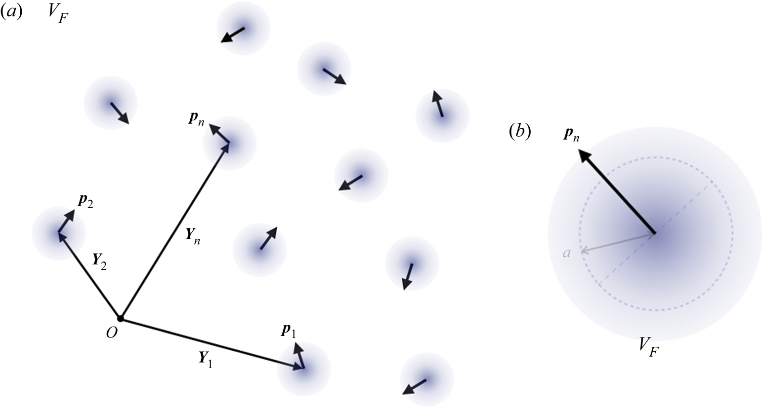
 $V_f$ and may be bounded or unbounded (figure 1a).
(a) Geometric description and parameter definition for (a) a reactive suspension system and (b) an individual active particle including the fluid domain  $V_f$, as well the phoretic particle’s position
 $\boldsymbol {Y}_n$ and orientation
 $\boldsymbol {p}_n$, for radius
 $a$. The particle's orientation
 $\boldsymbol {p}_n$, allows for the definition of its front caps (noted
 $F$ and
 $B$ respectively). The different colours of the caps (white or grey) illustrate their different chemical activities, while their patterns (striped and solid) illustrate their different mobilities.

Each particle emits a chemical solute of diffusivity  $D$ on the catalytic parts of its surface with a fixed spatially dependent rate, of characteristic magnitude
 $\alpha _0$, and is able to generate a slip flow in response to a surface concentration gradient, with a characteristic phoretic mobility
 $M_0$. In the following, all variables and equations are made dimensionless using
 $a$,
 $U_0=\alpha _0 M_0/D$ and
 $a\alpha _0/D$ as characteristic length, velocity and concentration scales.
As a result of its surface activity, the dimensionless relative concentration  $c$ (with respect to its background value far from the particles) satisfies the following Neumann condition on the surface of particle
 $n$:
 \begin{equation} {-}\boldsymbol{n} \boldsymbol{\cdot}\boldsymbol{\nabla} c = \alpha_n(\boldsymbol{n}) \quad \mathrm{on}\ S_n, \end{equation}
where  $\alpha _n(\boldsymbol {n})$ is the dimensionless activity distribution (i.e. emission rate) and
 $\boldsymbol {n}$ is the outward normal unit vector on
 $S_n$. For sufficiently small particles, the solute's dynamics is purely diffusive, i.e. the relevant Péclet number
 ${{Pe}=aU_0/D\ll 1}$, so that
 $c$ obeys Laplace's equation outside the particles,
 \begin{equation} \nabla^2 c = 0 \quad \mathrm{in}\ V_f. \end{equation}
Together with an appropriate boundary conditions at the external boundary of  $V_f$ (e.g.
 $c\rightarrow 0$ for
 $|\boldsymbol {r}|\rightarrow \infty$ in unbounded domains), these equations form a well-posed problem for the distribution of solute in the fluid domain
 $V_f$.
In response to a non-uniform solute distribution at the particles’ surface, a phoretic slip flow  $\boldsymbol {u}^s_n$ develops outside a thin interaction layer (Anderson Reference Anderson1989) so that, effectively, the hydrodynamic boundary condition on
 $S_n$ becomes
 \begin{equation} \boldsymbol{u} = \boldsymbol{U}_n + \boldsymbol{\varOmega}_n \times \boldsymbol{r}_n + \boldsymbol{u}^s_n,\quad \textrm{with } \boldsymbol{u}_n^s=M_n(\boldsymbol{n}) \nabla_{{\parallel}} c\quad \mathrm{on}\ S_n. \end{equation}
In the previous equation,  $\nabla _{\parallel }=({\boldsymbol{\mathsf{I}}}-\boldsymbol {n}\boldsymbol {n}) \boldsymbol {\cdot }\boldsymbol {\nabla }$ is the tangential gradient on the particle's surface,
 $\boldsymbol {r}_n=\boldsymbol {r}-\boldsymbol {Y}_n$ is the generic position relative to the centre of particle
 $n$ and
 $M_n(\boldsymbol {n})$ denotes the dimensionless and spatially dependent phoretic mobility of the surface of particle
 $n$. For small particles, inertial effects are negligible (i.e. the relevant Reynolds number
 ), and the dimensionless fluid's velocity and pressure (
 $\boldsymbol {u}, p$) satisfy the Stokes equations
 \begin{equation} \boldsymbol{\nabla} p = \nabla^2 \boldsymbol{u},\quad \boldsymbol{\nabla}\boldsymbol{\cdot} \boldsymbol{u}=0 \quad \mathrm{in}\ V_f, \end{equation}
with an appropriate condition at the outer boundary of  $V_f$ (e.g.
 $\boldsymbol {u}\rightarrow 0$ for
 $|\boldsymbol {r}|\rightarrow \infty$). Neglecting any outer forcing, such as gravity, each particle is hydrodynamically force and torque free (Popescu et al. Reference Popescu, Uspal and Dietrich2016) at all times,
 \begin{equation} \boldsymbol{F}_n = \int_{S_n} \boldsymbol{\sigma} \cdot \boldsymbol{n} \,\mathrm{d}S = \boldsymbol{0},\quad \boldsymbol{T}_n = \int_{S_n} \boldsymbol{r}_n \times (\boldsymbol{\sigma} \cdot \boldsymbol{n})\,\mathrm{d}S = \boldsymbol{0}, \end{equation}
with  $\boldsymbol \sigma =-p\boldsymbol {I}+(\boldsymbol {\nabla }\boldsymbol {u}+\boldsymbol {\nabla }\boldsymbol {u}^\textrm {T})$ the dimensionless Newtonian stress tensor, and their dominant hydrodynamic signature is therefore that of a force dipole or stresslet
 ${\boldsymbol{\mathsf{S}}}_n$ (Batchelor Reference Batchelor1970).
For a given concentration distribution  $c$, (2.3)–(2.5a,b) form a well-posed problem for the fluid velocity and pressure, and particle velocities, so that, at a given time
 $t$, and for given particle positions and orientations,
 $\boldsymbol {Y}_n(t)$ and
 $\boldsymbol {p}_n(t)$, the successive Laplace and Stokes problems presented above uniquely determine the instantaneous particle velocities
 $\boldsymbol {U}_n(t)$ and
 $\boldsymbol {\varOmega }_n(t)$, from which the motion of the particles is obtained
 \begin{equation} \frac{\mathrm{d}\boldsymbol{Y}_n}{\mathrm{d}t} = \boldsymbol{U}_n,\quad \frac{\mathrm{d}\boldsymbol{p}_n}{\mathrm{d}t} = \boldsymbol{\varOmega}_n \times \boldsymbol{p}_n. \end{equation}
For a single isolated particle, the Lorentz reciprocal theorem to Stokes flows provides the particle's translation and rotation velocities directly in terms of the phoretic slip (Stone & Samuel Reference Stone and Samuel1996)
 \begin{equation} \boldsymbol{U} ={-} \langle \boldsymbol{u}^s \rangle,\quad \boldsymbol{\varOmega} ={-}\frac{3}{2a}\langle \boldsymbol{n} \times \boldsymbol{u}^s \rangle, \end{equation}
where  $\langle \cdot \rangle$ is the spatial average over the particle's surface. Similarly, the stresslet
 ${\boldsymbol{\mathsf{S}}}$ of the particle is obtained as (Lauga & Michelin Reference Lauga and Michelin2016),
 \begin{equation} {\boldsymbol{\mathsf{S}}} ={-}10{\rm \pi} a^2 \langle \boldsymbol{n} \boldsymbol{u}^s +\boldsymbol{u}^s \boldsymbol{n} \rangle. \end{equation}
2.2. Hemispheric Janus phoretic particles
Most phoretic particles have a Janus-type surface consisting of two different materials or surface coatings with distinct physico-chemical properties (e.g. a catalytic side and a passive one) (Paxton et al. Reference Paxton, Kistler, Olmeda, Sen, Angelo, Cao, Mallouk, Lammert and Crespi2004; Howse et al. Reference Howse, Jones, Ryan, Gough, Vafabakhsh and Golestanian2007; Theurkauff et al. Reference Theurkauff, Cottin-Bizonne, Palacci, Ybert and Bocquet2012). These provide the particles with a built-in chemical asymmetry that triggers the inhomogeneity of the concentration distribution at their surface at the heart of their self-propulsion. In the following, we thus consider such hemispheric Janus particles with uniform but distinct mobilities  $(M_n^F,M_n^B)$ and activities
 $(\alpha ^F_n,\alpha _n^B)$ on their front (F) and back (B) hemispheres, as defined with respect to their orientation
 $\boldsymbol {p}_n$ (figure 1b), e.g. the surface mobility of particle
 $n$ writes
 \begin{equation} M_n(\boldsymbol{n}) = \bar{M}_n + M^*_n \,\mathrm{sign}(\boldsymbol{p}_n \cdot \boldsymbol{n}), \end{equation}
with  $\bar {M}_n=(M_n^F+M_n^B)/2$ and
 $M_n^*=(M_n^F-M_n^B)/2$ the mean mobility and mobility contrast, and a similar definition for the spatially dependent activity
 $\alpha _n(\boldsymbol {n})$ at the particle's surface. The special case of a particle with uniform mobility thus corresponds to
 $\bar {M}_n=M^0_n$ and
 $M^*_n=0$.
3. An FCM-based method for phoretic suspensions
In the purely diffusive and viscous limit, solving for the particles’ dynamics therefore amounts to solving sequentially two linear problems, namely a Laplace problem for  $c$ and a Stokes swimming problem for the hydrodynamic field and particles’ velocity. Although the exact solution to this joint problem can be obtained analytically for the single- and two-particle cases (Golestanian et al. Reference Golestanian, Liverpool and Ajdari2007; Sharifi-Mood et al. Reference Sharifi-Mood, Mozzafari and Córdova-Figueroa2016; Varma & Michelin Reference Varma and Michelin2019), analytical treatment becomes intractable beyond
 $N\geq 3$ due to the geometric complexity of the fluid domain, despite the problem's linearity. Numerical simulations are therefore critically needed, and several numerical strategies have been proposed recently and briefly reviewed in the introduction. In order to analyse accurately the collective dynamics of in a suspension of Janus phoretic particles, such a method must combine an efficient solution of the Laplace and Stokes problems outside a large number of finite-size objects, while providing accurate representation of the coupling at the surface of each particle between chemical and hydrodynamic fields.
With that double objective in mind, we propose and present here a novel numerical framework to solve for the reactive suspension problem presented in § 2, based on the classical FCM used for pure hydrodynamic simulations of passive particles or microswimmers, thereby generalizing its application to the solution of the chemical diffusion problem and its coupling with the already-established hydrodynamic FCM (Maxey & Patel Reference Maxey and Patel2001; Lomholt & Maxey Reference Lomholt and Maxey2003; Yeo & Maxey Reference Yeo and Maxey2010; Delmotte et al. Reference Delmotte, Keaveny, Plouraboué and Climent2015). Section 3.1 develops the regularized Laplace problem and associated reactive FCM, while § 3.2 presents a brief review of the existing hydrodynamic FCM and § 3.3 combines both to obtain a new DFCM approach.
The fundamental idea of the FCM is to replace a solution of the Stokes equations only within the fluid domain  $V_f$ outside the forcing particles, by a solution of these equations over the entire domain
 ${V_F=V_f\cup V_1\cup \cdots \cup V_N}$ (i.e. both outside and inside the particles), replacing the surface boundary conditions with a distributed regularized forcing over a compact envelope calibrated so as to reproduce certain physical features of the problem and account for a weak form of the surface boundary conditions (figure 2). Doing so, the costly discrete resolution and time-dependent meshing of the particles is no longer necessary, so that efficient (e.g. spectral) Laplace and Stokes solvers on a fixed regular grid may be used at all times, offering significant performance and scalability advantages with respect to other approaches (e.g. boundary element methods). More specifically, FCM associates with each particle a finite set of regularized hydrodynamic singularities (force monopoles, dipoles and so on) chosen so as to satisfy a weak form of the surface boundary conditions.
Regularized representation of (a) the reactive suspension system and (b) individual particles in the DFCM framework. The chemical and hydrodynamic fields are now defined over the entire domain with distributed forcings defined relative to each particle's position  $\boldsymbol {Y}_n$ and orientation
 $\boldsymbol {p}_n$. The boundary
 $S_n$ of the real particle (dashed) and its radius
 $a$ are plotted only as reference.

3.1. Reactive FCM
We extend here this approach to the solution of the Laplace problem for  $c$ in (2.1) and (2.2). Replacing each particle by a distributed forcing modifies Laplace's equations into a Poisson equation over the entire domain
 $V_F$ (including both fluid and particles),
 \begin{equation} \nabla^2 c ={-}g(\boldsymbol{r},t) \quad \mathrm{in}\ V_F, \end{equation}
where the function  $g(\boldsymbol {r},t)$ includes the source terms accounting for the presence of each particle.
3.1.1. Standard multipole expansion for Laplace problem
The exact solution of the Laplace problems can in fact be recovered from (3.1), when the function  $g(\boldsymbol {r},t)$ is taken as a (possibly infinite) set of singularities centred on each particle (Saffman Reference Saffman1973),
 \begin{equation} g(\boldsymbol{r},t) = \sum_{n=1}^N [q^M_n \delta(\boldsymbol{r}_n) {-} \boldsymbol{q}^D_n \boldsymbol{\cdot}\boldsymbol{\nabla}\delta(\boldsymbol{r}_n) + \cdots], \end{equation}
where  $\delta (\boldsymbol {r}_n)$ is the Dirac delta distribution, and (
 $q_n^M$,
 $\boldsymbol {q}_n^D,\ldots$) are the intensities of the singularities associated with particle
 $n$, and are constant tensors of increasing order. Note that
 $\boldsymbol {\nabla }$ denotes here the gradient with respect to the observation position
 $\boldsymbol {r}$ and
 $\boldsymbol {r}_n=\boldsymbol {r}-\boldsymbol {Y}_n$. This equation can be solved explicitly for the concentration field
 $c$ as a multipole expansion for each particle in terms of source monopoles, dipoles, etc
 $\ldots$
 \begin{equation} c(\boldsymbol{r},t) = \sum_{n=1}^N [q^M_n G^M(\boldsymbol{r}_n) + \boldsymbol{q}^D_n \cdot \boldsymbol{G}^D(\boldsymbol{r}_n) + \cdots], \end{equation}
where  $G^M$ and
 $\boldsymbol {G}^D$ are the monopole and dipole Green's functions and satisfy
 \begin{equation} \nabla^2 G^M={-}\delta(\boldsymbol{r}_n),\quad \nabla^2 \boldsymbol{G}^D= \boldsymbol{\nabla}\delta(\boldsymbol{r}_n), \end{equation}
together with appropriate decay or boundary conditions on the domain's outer boundary. For unbounded domains with decaying conditions in the far field, the singular monopole and dipole Green's functions are simply
 \begin{equation} G^M(\boldsymbol{r}_n) = \frac{1}{4{\rm \pi} r_n}\quad \textrm{and}\quad \boldsymbol{G}^D(\boldsymbol{r}_n)={-}\boldsymbol{\nabla} G^M =\frac{\boldsymbol{r}_n}{4{\rm \pi} r_n^3}\cdot. \end{equation}
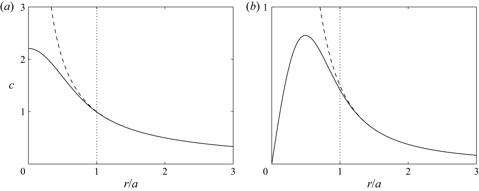
The concentration distributions associated with these singular Green's functions are displayed in figure 3. Higher-order derivatives of  $G^M(\boldsymbol {r})$, (3.5a,b), are also solutions of Laplace's equation, leading to singularities of increasing order (quadrupole, octupole,…).
Singular (dotted lines, (3.5a,b)) and regularized (solid lines, (3.10)–(3.11)) concentration distributions along the axial polar direction associated with the Greens’ functions for the Laplace equation for (a) monopole terms and (b) dipole terms. The line  $r/a=1$ represents the particle surface.

3.1.2. Truncated regularized multipole expansion
The previous approach, based on an infinite set of singular sources, is known as the standard multipole expansion of the Laplace problem. Although satisfying from a theoretical point of view, since it is able to recover an accurate representation of the analytical solution outside the particles for a large enough number of singular multipoles, it is not well suited for a versatile numerical implementation because of (i) the singular behaviour of the forcing terms in the modified Laplace equation, (3.1), and (ii) the a priori infinite set of singularities required for each particle.
To avoid the latter issue, the infinite expansion is truncated here after the first two terms, thus retaining the monopole and dipole contributions only. Physically, this amounts to retaining the two leading physical effects of the particle on the concentration field, i.e. a net emission with a front–back asymmetric distribution. In order to overcome the former problem, the standard FCM replaces the singular Dirac distributions  $\delta (\boldsymbol {r})$ by regular Gaussian spreading functions
 $\varDelta (\boldsymbol {r})$:
 \begin{equation} \triangle(\boldsymbol{r}) = (2{\rm \pi}\sigma^2)^{{-}3/2} \exp\left(-\frac{r^2}{2\sigma^2}\right), \end{equation}
where  $\sigma$ denotes the finite-size support of this envelop and acts as a smoothing parameter of the method, thus eliminating the singular behaviour of the delta distribution
 $\delta (\boldsymbol {r})$ near the origin, thereby allowing for a more accurate numerical treatment. The original singular distribution is recovered when
 $\sigma \ll r$, i.e. the solution of the regularized problem is an accurate representation of the true solution away from the particle. This approach using regular distributions allows for a more versatile and robust numerical solution of the physical equations than their singular counterparts (Maxey & Patel Reference Maxey and Patel2001; Lomholt & Maxey Reference Lomholt and Maxey2003).
Combining these two approximations, we therefore consider a truncated regularized expansion including only the monopole and the dipole terms as
 \begin{equation} g(\boldsymbol{r},t) = \sum_{n=1}^N [q^M_n \varDelta^M({r}_n) {-} \boldsymbol{q}^D_n \boldsymbol{\cdot}\boldsymbol{\nabla} \varDelta^D({r}_n)], \end{equation}
with the Gaussian spreading operators  $\varDelta ^M$ and
 $\varDelta ^D$ defined as
 \begin{equation} \varDelta^M(r) = (2{\rm \pi}\sigma_M^2)^{{-}3/2} \exp\left(-\frac{r^2}{2 \sigma_M^2}\right),\quad \varDelta^D(r) = (2{\rm \pi}\sigma_D^2)^{{-}3/2} \exp\left(-\frac{r^2}{2 \sigma_D^2}\right), \end{equation}
where  $M$ and
 $D$ once again denote monopole and dipole, and
 $\sigma _M$ and
 $\sigma _D$ are the finite support of each regularized distribution and are free numerical parameters of the method that need to be calibrated. Note that, in general, these do not need to be identical (Lomholt & Maxey Reference Lomholt and Maxey2003).
The corresponding truncated regularized solution for  $c$ is then finally obtained as
 \begin{equation} c(\boldsymbol{r},t) = \sum_{n=1}^N [q^M_n G^M(\boldsymbol{r}_n) + \boldsymbol{q}^D_n \cdot \boldsymbol{G}^D(\boldsymbol{r}_n)], \end{equation}
with the regularized monopole and dipole Green's functions
 $$\begin{gather} G^M(\boldsymbol{r}) = \frac{1}{4{\rm \pi} r} \mathrm{erf}\left( \frac{r}{{\sigma_M}\sqrt{2}} \right), \end{gather}$$
 $$\begin{gather}\boldsymbol{G}^D(\boldsymbol{r})= \frac{\boldsymbol{r}}{4{\rm \pi} r^3} \left[\mathrm{erf}\left(\frac{r}{\sigma_D \sqrt{2}}\right) -\sqrt{\frac{2}{\rm \pi}} \left(\frac{r}{\sigma_D}\right) \exp\left(-\frac{r^2}{2\sigma_D^2}\right)\right]. \end{gather}$$
These clearly match the behaviour of their singular counterpart, (3.5a,b), when  $r$ is greater than a few
 $\sigma _M$ or
 $\sigma _D$, respectively, while still maintaining finite values within the particle (figure 3), e.g.
 $\boldsymbol {G}^D(\boldsymbol {r}=\boldsymbol {0})=\boldsymbol {0}$.
3.1.3. Finding the intensity of the singularities
Up to this point, no information was implemented regarding the surface boundary conditions on  $c$ in (2.1). We now present how to determine the intensities of the monopole and dipole distributions associated with each particle,
 $q^M_n$ and
 $\boldsymbol {q}^D_n$, so as to satisfy a weak form of the Neuman boundary condition, (2.1), i.e. its first two moments over the particle's surface. Using the multipole expansion of the fundamental integral representation of the concentration (see Appendix A), the monopole and dipole intensities of particle
 $n$,
 $q^M_n$ and
 $\boldsymbol {q}^{D}_n$, are obtained as (Yan & Brady Reference Yan and Brady2016)
 \begin{equation} q^M_n = \int_{S_n} \alpha_n \mathrm{d}S,\quad \boldsymbol{q}^{D}_n = a \int_{S_n} \alpha_n \boldsymbol{n}\,\mathrm{d}S + 4{\rm \pi} a^2 \langle c \boldsymbol{n} \rangle_n, \end{equation}
where the second term in  $\boldsymbol {q}_n^D$ is proportional to the concentration polarity at the surface of particle
 $n$, i.e. its first moment
 $\langle c \boldsymbol {n} \rangle _n$, and is defined using the surface average operator
 $\langle \cdot \rangle _n$ over the surface of particle
 $n$. Note that the activity distribution at the particle's surface is known, and thus (2.9) explicitly provides the monopole intensity and the first term in the dipole intensity. The second contribution to the latter requires, however, knowledge of the solution on the particle's surface – which is not explicitly represented in the present FCM approach. This term therefore requires to be solved for as part of the general problem. In the previous equation, it should be noted that the dimensionless particle radius is
 $a=1$, but will be kept in the equations to emphasize the relative scaling of the numerical spreading envelopes (e.g.
 $\sigma _M$ and
 $\sigma _D$) with respect to the particle size.
Here, we use an iterative approach to solve this linear joint problem for the dipole intensity and concentration field, solving alternatively (3.7) and (3.12a,b) until convergence is reached, as defined by the following criterion between two successive iterations:
 \begin{equation} \left\| \frac{ \langle c\boldsymbol{n}\rangle^{k+1}- \langle c\boldsymbol{n}\rangle^{k}}{\langle c\boldsymbol{n}\rangle^{k+1}}\right\|_{\infty} < \epsilon, \end{equation}
where  $\langle c\boldsymbol {n}\rangle ^{k}$ is the vector collecting the polarities of the
 $N$ particles at iteration
 $k$. For the results presented in this work, we set the tolerance to
 $\epsilon =10^{-10}$ in our calculations.
3.1.4. Regularized moments of the concentration distribution
Finding the dipole intensity,  $\boldsymbol {q}^{D}_n$, requires computing the polarity
 $\langle c \boldsymbol {n} \rangle _n$, which is in principle defined at the particle's surface. To follow the spirit of FCM, and allow for efficient numerical treatment, this surface projection is replaced by a weighted projection over the entire volume
 $V_F$
 \begin{equation} \langle c \boldsymbol{n} \rangle_n =\frac{1}{4{\rm \pi} a^2} \int_{S_n} c \boldsymbol{n} \mathrm{d}S \quad\longrightarrow\quad \{ c \boldsymbol{n} \}_n = \int_{V_F} c \boldsymbol{n}_n \varDelta^P(\boldsymbol{r}_n)\,\mathrm{d}V, \end{equation}
with  $\boldsymbol {n}_n$ now defined as
 $\boldsymbol {n}_n={\boldsymbol {r}_n}/{r_n}$, and the regular averaging kernel
 $\varDelta ^P$ for the polarity as
 \begin{equation} \varDelta^P(\boldsymbol{r}) = \frac{r}{8{\rm \pi}\sigma_P^4} \exp\left(-\frac{r^2}{2 \sigma_P^2}\right). \end{equation}
Beyond its importance for determining the dipole intensity associated with a given particle, we will later show that the polarity of the concentration at the surface of particle  $n$ is directly related to its self-induced phoretic velocity, (2.7a,b), and that, similarly, the self-induced hydrodynamic stresslet signature of the particle is in general associated with the first two moments of the surface concentration. Similarly to the polarity, the second surface moment,
 $\langle c(\boldsymbol {n}\boldsymbol {n}-{\boldsymbol{\mathsf{I}}}/3) \rangle _n$ will be replaced in our implementation by a weighted volume projection
 $\{c(\boldsymbol {n}\boldsymbol {n}-{\boldsymbol{\mathsf{I}}}/3)\}_n$
 \begin{align} \langle c(\boldsymbol{n}\boldsymbol{n}-{\boldsymbol{\mathsf{I}}}/3) \rangle_n &= \frac{1}{4{\rm \pi} a^2}\int_{S_n}c\left(\boldsymbol{n}\boldsymbol{n}-\frac{{\boldsymbol{\mathsf{I}}}}{3}\right)\mathrm{d}S \rightarrow \{ c(\boldsymbol{n}\boldsymbol{n}-{\boldsymbol{\mathsf{I}}}/3) \}_n \nonumber\\ &= \int_{V_F} c \left(\boldsymbol{n}_n\boldsymbol{n}_n-\frac{{\boldsymbol{\mathsf{I}}}}{3}\right) \varDelta^S(\boldsymbol{r}_n)\,\mathrm{d}V, \end{align}
where the projection kernel for the second moment of concentration,  $\varDelta ^S$, is defined as
 \begin{equation} \varDelta^S(\boldsymbol{r})= \frac{r^2}{3(2{\rm \pi})^{{3}/{2}} \sigma_S^5} \exp\left(-\frac{r^2}{2 \sigma_S^2}\right). \end{equation}
The envelopes  $\sigma _P$ and
 $\sigma _S$ are free parameters in the method that need to be calibrated. In our reactive FCM formulation, we use modified forms of the Gaussian operator
 $\varDelta$ as projection operators, (3.15) and (3.17), in order to ensure a fast numerical convergence of the integration for the first and second moment calculations, (3.14) and (3.16) respectively. The integrals over the entire volume
 $V_F$ of these averaging functions is still equal to one, and their weight is shifted from the particle centre toward the particle surface (figure 4), which is both numerically more accurate and more intuitive physically as these operators are used to obtain the properties of the particle on its surface.


3.1.5. Calibrating the spreading/averaging envelopes
Our method relies on four numerical parameters ( $\sigma _M$,
 $\sigma _D$,
 $\sigma _P$,
 $\sigma _S$) that we choose to calibrate so as to ensure that several key results in reference configurations are obtained exactly. In particular, to properly account for the phoretic drift induced by the other particles, we ensure that the polarity
 $\langle c\boldsymbol {n}\rangle$ of an isolated particle placed in an externally imposed uniform gradient of concentration can be exactly recovered using the regular representation and averaging operators. A similar approach is then followed for the particle's second moment of concentration
 $\langle c(\boldsymbol {n}\boldsymbol {n}-{\boldsymbol{\mathsf{I}}}/3)\rangle$ in a quadratic externally imposed field.
Isolated passive particle in an external linear field – We first consider a single particle placed at the origin in an externally imposed linear concentration field so that for  $r\gg a$,
 $c\approx c_E$ with
 \begin{equation} c_E = \boldsymbol{L}_E \cdot \boldsymbol{r}, \end{equation}
where  $\boldsymbol {L}_E$ is the externally imposed uniform gradient. For a passive particle (i.e.
 $\alpha =0$), satisfying the boundary condition, (2.1), at the surface of the particle imposes that the exact concentration distribution around the particle is
 $c=c_E+c_I^o$, with
 ${c_I^o(\boldsymbol {r})=a^3\boldsymbol {L}_E\cdot \boldsymbol {r}/(2r^3)}$ a singular dipole-induced field. The polarity of the external and induced parts,
 $c_E$ and
 $c_I$, can be obtained analytically as
 \begin{equation} \langle c_E \boldsymbol{n} \rangle = \frac{a}{3}\boldsymbol{L}_E,\quad \langle c_I^o \boldsymbol{n} \rangle = \frac{a}{6}\boldsymbol{L}_E. \end{equation}
Following the framework presented above, the regularized solution can be written  $c=c_E+c_I^r$ with
 $c_i^r$ a regularized dipole, and the corresponding regularized-volume moments based on (3.14) are obtained using (3.11), as
 \begin{equation} \{ c_E \boldsymbol{n} \} = \sqrt{\frac{\rm \pi}{8}} \sigma_P \boldsymbol{L}_E,\quad \{ c_I^r \boldsymbol{n} \} = \frac{a^3\sigma_P}{12(\sigma_D^2+\sigma_P^2)^{{3}/{2}}} \boldsymbol{L}_E. \end{equation}
Identification of the regularized result (3.20a,b) with the true solution (3.19a,b), determines  $\sigma _P$ and
 $\sigma _D$ uniquely as
 \begin{equation} \frac{\sigma_P}{a}=\frac{1}{3}\sqrt{\frac{8}{\rm \pi}} \approx 0.5319,\quad \frac{\sigma_D}{a} = \sqrt{\left(\frac{\sigma_P}{2a}\right)^{2/3} - \left(\frac{\sigma_P}{a}\right)^{2}} \approx 0.3614. \end{equation}
Isolated passive particle in an external quadratic field – Similarly, in an external quadratic field  $c_E$ of the form
 \begin{equation} c_E(\boldsymbol{r})= \boldsymbol{r} \cdot {\boldsymbol{\mathsf{Q}}}_E \cdot \boldsymbol{r}, \end{equation}
with  ${\boldsymbol{\mathsf{Q}}}_E$ a second-order symmetric and traceless tensor, the concentration distribution around a passive particle (
 $\alpha =0$) takes the form
 $c=c_E+c_I^o$ with
 $c_I^o(\boldsymbol {r})$ an induced singular quadrupole. The exact and regularized second moments of the external field
 $c_E$ at the particle surface are equal to
 \begin{equation} \langle c_E (\boldsymbol{n}\boldsymbol{n}-{\boldsymbol{\mathsf{I}}}/3) \rangle = \frac{2a^2}{15}{\boldsymbol{\mathsf{Q}}}_E,\quad \{c_E (\boldsymbol{n}\boldsymbol{n}-{\boldsymbol{\mathsf{I}}}/3) \} = \frac{2\sigma_S^2}{3}{\boldsymbol{\mathsf{Q}}}_E. \end{equation}
Identifying both results determines the size of the averaging envelope for the second moment uniquely, as
 \begin{equation} \frac{\sigma_S}{a}=\sqrt{\frac{1}{5}} \approx 0.4472. \end{equation}
Note that we do not enforce here a constraint on the representation of the second moment of the induced field  $c_I$, since the particles’ representations do not include a regularized quadrupole in our method.
The value  $\sigma _M$ remains as a free parameter at this point and cannot be calibrated with a similar approach. In the following, in order to minimize the number of distinct numerical parameters and to minimize the departure of the regularized solution from its singular counterpart, we set its value equal to the smallest envelope size, namely
 $\sigma _M=\sigma _D$. These specific values of the parameters were used in figures 3 and 4.
3.2. Hydrodynamic FCM
To compute the hydrodynamic interactions between phoretic particles, we rely on the FCM. This section briefly describes the existing FCM framework developed for the simulation of passive and active suspensions in Stokes flow.
3.2.1. FCM for passive suspensions
With hydrodynamic FCM, the effect of the particles on the fluid is accounted for through a forcing term  $\boldsymbol {f}$ applied to the dimensionless Stokes equations
 \begin{equation} \boldsymbol{\nabla} p - \nabla^2 \boldsymbol{u}= \boldsymbol{f}(\boldsymbol{r},t) \quad \mathrm{in}\ V_F. \end{equation}
As for reactive FCM, this forcing arises from a truncated regularized multipolar expansion up to the dipole level
 \begin{equation} \boldsymbol{f}(\boldsymbol{r},t) = \sum_{n=1}^N [\boldsymbol{F}_n \varDelta (r_n) + {\boldsymbol{\mathsf{D}}}_n \boldsymbol{\cdot}\boldsymbol{\nabla} \varDelta^*(r_n)], \end{equation}
where the spreading envelopes are defined by
 \begin{equation} \varDelta(r) = (2{\rm \pi}\sigma^2)^{{-}3/2} \exp\left(-\frac{r^2}{2 \sigma^2}\right),\quad \varDelta^*(r) = (2{\rm \pi}\sigma_*^2)^{{-}3/2} \exp\left(-\frac{r^2}{2 \sigma_*^2}\right). \end{equation}
Here,  $\boldsymbol {F}_n$ and
 ${\boldsymbol{\mathsf{D}}}_n$ are the force monopole and dipole applied to particle
 $n$. The force dipole can be split into a symmetric part, the stresslet
 ${\boldsymbol{\mathsf{S}}}$, and an antisymmetric one related to the external torque
 $\boldsymbol {T}$
 \begin{equation} {\boldsymbol{\mathsf{D}}}_n = {\boldsymbol{\mathsf{S}}}_n + \tfrac{1}{2} \boldsymbol{\epsilon} \cdot \boldsymbol{T}_n, \end{equation}
with  $\boldsymbol{\epsilon}$ the third-order permutation tensor. The corresponding regularized solution for the fluid velocity
 $\boldsymbol {u}$ is then obtained as
 \begin{equation} \boldsymbol{u} = \boldsymbol{u}(\boldsymbol{r}) = \sum_{n=1}^{N} [\boldsymbol{F}_n \cdot {\boldsymbol{\mathsf{J}}} (\boldsymbol{r}_n)+ {\boldsymbol{\mathsf{D}}}_n : {\boldsymbol{\mathsf{R}}}^*(\boldsymbol{r}_n)]. \end{equation}
For unbounded domains with vanishing perturbations in the far field (i.e.  $\|\boldsymbol {u}\|\rightarrow 0$ when
 $r \rightarrow \infty$), the regularized Green's function
 ${\boldsymbol{\mathsf{J}}}(\boldsymbol {r})$ reads
 \begin{equation} {\boldsymbol{\mathsf{J}}}(\boldsymbol{r}) = \frac{1}{8 {\rm \pi}r} \left(A(r) {\boldsymbol{\mathsf{I}}} + B(r) \frac{\boldsymbol{r}\boldsymbol{r}}{r^2}\right), \end{equation}
with
 $$\begin{gather} A(r)= \left(1+\frac{\sigma^2}{r^2}\right) \mathrm{erf}\left(\frac{r}{\sigma \sqrt{2}}\right) - \frac{\sigma}{r} \sqrt{\frac{2}{\rm \pi}} \exp\left(-\frac{r^2}{2\sigma^2}\right), \end{gather}$$
 $$\begin{gather}B(r)= \left(1-\frac{3\sigma^2}{r^2}\right) \mathrm{erf}\left(\frac{r}{\sigma \sqrt{2}}\right) + \frac{3\sigma}{r}\sqrt{\frac{2}{\rm \pi}} \exp\left(-\frac{r^2}{2\sigma^2}\right), \end{gather}$$
and  ${\boldsymbol{\mathsf{R}}}^*=\boldsymbol {\nabla } {\boldsymbol{\mathsf{J}}}^*$ is the FCM dipole Green's function evaluated with the parameter
 $\sigma _*$.
The particle's translational and angular velocities,  $\boldsymbol {U}_n$ and
 $\boldsymbol {\varOmega }_n$, are obtained from a volume-weighted average of the local fluid velocity and vorticity
 \begin{equation} \boldsymbol{U}_n = \int_{V_F} \boldsymbol{u} \varDelta(\boldsymbol{r}_n)\,\mathrm{d}V,\quad \boldsymbol{\varOmega}_n = \tfrac{1}{2}\int_{V_F} [\boldsymbol{\nabla} \times \boldsymbol{u}] \varDelta^*(\boldsymbol{r}_n)\,\mathrm{d}V. \end{equation}
The Gaussian parameters,  $\sigma$ and
 $\sigma ^*$, are calibrated to recover the correct Stokes drag,
 ${\boldsymbol {F}=6{\rm \pi} a \mu \boldsymbol {U}}$, and viscous torque,
 $\boldsymbol {T}=8{\rm \pi} a^3 \mu \boldsymbol {\varOmega }$, of an isolated particle (Maxey & Patel Reference Maxey and Patel2001; Lomholt & Maxey Reference Lomholt and Maxey2003), leading to
 \begin{equation} \frac{\sigma}{a} =\frac{1}{\sqrt{\rm \pi}} \approx 0.5641,\quad \frac{\sigma_*}{a}=\frac{1}{(6\sqrt{\rm \pi})^{1/3}} \approx 0.4547. \end{equation}
The rigidity of the particle is similarly weakly enforced by imposing that the volume-averaged strain rate  ${\boldsymbol{\mathsf{E}}}_n$ over the envelope of particle
 $n$ vanishes
 \begin{equation} {\boldsymbol{\mathsf{E}}}_n = \tfrac{1}{2} \int_{V_F} [\boldsymbol{\nabla} \boldsymbol{u} + (\boldsymbol{\nabla} \boldsymbol{u})^\mathrm{T}] \varDelta^*(\boldsymbol{r}_n)\,\mathrm{d}V = \boldsymbol{0}, \end{equation}
which determines the stresslet  ${\boldsymbol{\mathsf{S}}}_n$ induced by particle
 $n$. Note that, unlike forces and torques which are typically set by external or inter-particle potentials, the stresslets result from the constraint on the flow given by (3.35) and, consequently, need to be solved for as part of the general flow problem. The resulting linear system for the unknown stresslet coefficients is solved directly or iteratively, with the conjugate gradients method, depending on the number of particles considered (Lomholt & Maxey Reference Lomholt and Maxey2003; Yeo & Maxey Reference Yeo and Maxey2010). In the following, we consider pairs of particles (see § 4) and therefore use direct inversion.
Note that the averaging envelopes used to recover the translational and rotational velocities,  $\triangle _n$ and
 $\triangle ^*_n$, are exactly the same as the spreading operators in (3.26), all of them Gaussian functions. As a result, the spreading and averaging operators are adjoints to one another. Also note that only two envelope lengths are required for the hydrodynamic problem:
 $\sigma$ and
 $\sigma _*$. In contrast, the new reactive FCM extension presented in § 3.1 uses spreading and averaging operators that are not adjoint. To recover the first (3.14) and second (3.16) moments of concentration we have two non-Gaussian averaging envelopes (
 $\varDelta ^P$ and
 $\varDelta ^S$), that differ from the Gaussian spreading envelopes (
 $\varDelta ^M$ and
 $\varDelta ^D$) in (3.7). While having adjoint operators is crucial in hydrodynamic FCM to satisfy the fluctuation–dissipation balance, the lack of adjoint properties for the Laplace problem does not raise any issue in the deterministic setting.
3.2.2. Active hydrodynamic FCM
In recent years, FCM has been extended to handle suspensions of active particles, such as microswimmers. In addition to undergoing rigid body motion in the absence of applied forces or torques, active and self-propelled particles are also characterized by the flows they generate. These flows can be incorporated into FCM by adding an appropriate set of regularized multipoles to the Stokes equations. This problem was solved previously for the classical squirmer model (Delmotte et al. Reference Delmotte, Keaveny, Plouraboué and Climent2015), a spherical self-propelled particle that swims using prescribed distortions of its surface. In the most common case where radial distortions are ignored, the squirmer generates a tangential slip velocity on its surface, just like phoretic particles, which can be expanded into spherical harmonics modes (Blake Reference Blake1971; Pak & Lauga Reference Pak and Lauga2014). Consistently with the phoretic problem presented above, only the first two modes are included in the following.
The FCM force distribution produced by  $N$ microswimmers self-propelling with a surface slip velocity is given by
 \begin{equation} \boldsymbol{f}(\boldsymbol{r},t) = \sum_{n=1}^N [{\boldsymbol{\mathsf{S}}}_n \boldsymbol{\cdot} \boldsymbol{\nabla} \varDelta^*(r_n) + {\boldsymbol{\mathsf{S}}}^a_n \boldsymbol{\cdot}\boldsymbol{\nabla} \varDelta(r_n) + \boldsymbol{H}^a_n \nabla^2 \varDelta^*(r_n)], \end{equation}
where  ${\boldsymbol{\mathsf{S}}}^a_n$ is the active stresslet and
 $\boldsymbol {H}^a_n$ is the active potential dipole associated with the swimming disturbances of swimmer
 $n$. The latter is defined as
 \begin{equation} \boldsymbol{H}^a_n ={-}2 {\rm \pi}a^3 \boldsymbol{U}^a_n, \end{equation}
where  $\boldsymbol {U}^a_n$ is the swimming velocity arising from the slip velocity on the swimmer surface
 $\boldsymbol {u}^s$ (2.7a,b). Note that the rigidity stresslet
 ${\boldsymbol{\mathsf{S}}}_n$ is included in (3.36) to enforce the absence of deformation of the swimmers, (3.35). The resulting velocity field reads
 \begin{equation} \boldsymbol{u}(\boldsymbol{r},t) = \sum_{n=1}^{N} [{\boldsymbol{\mathsf{S}}}_n : {\boldsymbol{\mathsf{R}}}^*(\boldsymbol{r}_n) + {\boldsymbol{\mathsf{S}}}^a_n : {\boldsymbol{\mathsf{R}}}(\boldsymbol{r}_n) + \boldsymbol{H}^a_n \cdot {\boldsymbol{\mathsf{A}}}^*(\boldsymbol{r}_n) ], \end{equation}
where  ${\boldsymbol{\mathsf{R}}}$ is the FCM dipole Green's function evaluated with the parameter
 $\sigma$ instead of
 $\sigma _*$. The second-order tensor
 ${\boldsymbol{\mathsf{A}}}^*$ is the FCM Green's function for the potential dipole
 \begin{equation} {\boldsymbol{\mathsf{A}}}^*(\boldsymbol{r}) = \frac{1}{4{\rm \pi} r^3} \left[{\boldsymbol{\mathsf{I}}} - \frac{3\boldsymbol{r}\boldsymbol{r}}{r^2}\right] \mathrm{erf}\left(\frac{r}{\sigma_* \sqrt{2}}\right) - \frac{1}{\mu} \left[\left({\boldsymbol{\mathsf{I}}} - \frac{\boldsymbol{r}\boldsymbol{r}}{r^2} \right) + \left({\boldsymbol{\mathsf{I}}} - \frac{3\boldsymbol{r}\boldsymbol{r}}{r^2} \right) \left(\frac{\sigma_*}{r}\right)^2 \right] \varDelta^*(r). \end{equation}
The particles’ velocity, angular velocity and mean strain rate are then computed as
 $$\begin{gather} \boldsymbol{U}_n = \boldsymbol{U}^a_n -\boldsymbol{W}_n + \int_{V_F} \boldsymbol{u}\varDelta(\boldsymbol{r}_n) \,\mathrm{d}V, \end{gather}$$
 $$\begin{gather}\boldsymbol{\varOmega}_n = \boldsymbol{\varOmega}^a_n + \tfrac{1}{2}\int_{V_F} [\boldsymbol{\nabla} \times \boldsymbol{u}] \varDelta^*(\boldsymbol{r}_n)\,\mathrm{d}V, \end{gather}$$
 $$\begin{gather}{\boldsymbol{\mathsf{E}}}_n ={-}{\boldsymbol{\mathsf{K}}}_n + \tfrac{1}{2} \int_{V_F} [\boldsymbol{\nabla} \boldsymbol{u} + (\boldsymbol{\nabla} \boldsymbol{u})^\mathrm{T}] \varDelta^*(\boldsymbol{r}_n)\,\mathrm{d}V = \boldsymbol{0}, \end{gather}$$
where the active swimming velocities  $\boldsymbol {U}^a_n$ and rotation rates
 $\boldsymbol {\varOmega }^a_n$ correspond to the intrinsic velocities of particle
 $n$, if it was alone (i.e. in the absence of external flows or other particles), and
 $\boldsymbol {W}_n$ and
 ${\boldsymbol{\mathsf{K}}}_n$ are defined as
 $$\begin{gather} \boldsymbol{W}_n = \int_{V_F} [\boldsymbol{H}^a_n\cdot{\boldsymbol{\mathsf{A}}}^*(\boldsymbol{r}_n)] \varDelta(\boldsymbol{r}_n)\,\mathrm{d}V, \end{gather}$$
 $$\begin{gather}{\boldsymbol{\mathsf{K}}}_n = \tfrac{1}{2} \int_{V_F} [{\boldsymbol{\mathsf{S}}}^a_n:\boldsymbol{\nabla} {\boldsymbol{\mathsf{R}}}(\boldsymbol{r}_n) + ({\boldsymbol{\mathsf{S}}}_n^a:\boldsymbol{\nabla} {\boldsymbol{\mathsf{R}}}(\boldsymbol{r}_n))^\mathrm{T}] \varDelta^*(\boldsymbol{r}_n)\,\mathrm{d}V, \end{gather}$$
and are included to subtract away the spurious self-induced velocities and local rates of strain arising from the integration of the full velocity field  $\boldsymbol {u}$, which already includes the contribution of
 $\boldsymbol {H}^a_n$ and
 ${\boldsymbol{\mathsf{S}}}_n^a$ (Delmotte et al. Reference Delmotte, Keaveny, Plouraboué and Climent2015).
3.3. Diffusio-phoretic FCM
At this point, we have described our new reactive FCM framework and have reviewed the key aspects of the existing active hydrodynamic FCM. These two steps provide respectively the solution (i) for the concentration field and its moments at the surface of each particle in terms of their position and orientation, and (ii) the particles’ velocity in terms of their active hydrodynamic characteristics, i.e. their intrinsic velocities and stresslet,  $\boldsymbol {U}_n^a$,
 $\boldsymbol \varOmega _n^a$ and
 ${\boldsymbol{\mathsf{S}}}_n^a$. To solve for the full diffusio-phoretic problem (i.e. obtain the velocity of the particle in terms of their position and orientation), these quantities must be determined from the chemical environment of the particles. The following section details how to obtain these active characteristics from the output of the reactive problem and provides algorithmic details on the numerical implementation. This new diffusio-phoretic framework based on the FCM is referred to as DFCM hereafter.
3.3.1. DFCM: coupling reactive and hydrodynamic FCM
The active swimming speed  $\boldsymbol {U}^a_n$ involved in the potential dipole
 $\boldsymbol {H}^a_n$, (3.37), is the phoretic response of particle
 $n$ to the chemical field, if it was hydrodynamically isolated (i.e. neglecting the presence of other particles in solving the swimming problem). It thus includes its self-induced velocity (i.e. the response to the concentration contrasts induced by its own activity) and the drift velocity induced by the activity of the other particles. The swimming problem for a hydrodynamically isolated particle in unbounded flows can be solved directly using the reciprocal theorem (Stone & Samuel Reference Stone and Samuel1996), and using the definition of the phoretic slip flow
 \begin{equation} \boldsymbol{U}^a_n ={-} \langle \boldsymbol{u}^s \rangle_n ={-} \langle M \nabla_{{\parallel}} c \rangle_n. \end{equation}
After substitution of the mobility distribution at the surface of particle  $n$, (2.9), using a truncated multipolar expansion of the surface concentration on particle
 $n$ (up to its second-order moment) and integration by parts, the intrinsic swimming velocity is obtained in terms of the first two surface concentration moments (see Appendix B for more details)
 \begin{equation} \boldsymbol{U}^a_n ={-}\frac{2\bar{M}_n}{a} \langle c\boldsymbol{n} \rangle_n -\frac{15 M^*_n}{8a} [2 \langle c(\boldsymbol{n}\boldsymbol{n}-{\boldsymbol{\mathsf{I}}}/3) \rangle_n \cdot \boldsymbol{p}_n + \left( \langle c(\boldsymbol{n}\boldsymbol{n}-{\boldsymbol{\mathsf{I}}}/3) \rangle_n : \boldsymbol{p}_n\boldsymbol{p}_n \right) \boldsymbol{p}_n]. \end{equation}
Similarly, the active stresslet  ${\boldsymbol{\mathsf{S}}}^a_n$, is defined as in (2.8),
 \begin{equation} {\boldsymbol{\mathsf{S}}}^a_n ={-}10{\rm \pi} a^2 \langle \boldsymbol{n} \boldsymbol{u}^s +\boldsymbol{u}^s \boldsymbol{n} \rangle_n ={-}10{\rm \pi} a^2 \langle M ( \boldsymbol{n} \nabla_{{\parallel}} c + (\nabla_{{\parallel}} c) \boldsymbol{n} ) \rangle_n, \end{equation}
and rewrites in terms of the moments of concentration (see Appendix B for more details)
 \begin{align} {\boldsymbol{\mathsf{S}}}^a_n ={-}60 {\rm \pi}a \bar{M}_n \langle c(\boldsymbol{n}\boldsymbol{n}-{\boldsymbol{\mathsf{I}}}/3) \rangle_n + \frac{15 {\rm \pi}a M^*_n}{2} [(\langle c\boldsymbol{n} \rangle_n \cdot \boldsymbol{p}_n) ({\boldsymbol{\mathsf{I}}}-\boldsymbol{p}_n\boldsymbol{p}_n) - \langle c\boldsymbol{n} \rangle_n \boldsymbol{p}_n - \boldsymbol{p}_n \langle c\boldsymbol{n} \rangle_n]. \end{align}
Finally, the active rotation  $\boldsymbol {\varOmega }^a_n$, (2.7a,b), is obtained in terms of the moments of concentration and the mobility contrast (see Appendix B)
 \begin{equation} \boldsymbol{\varOmega}^a_n = -\frac{9M^*_n}{4a^2} \boldsymbol{p}_n \times \langle c\boldsymbol{n} \rangle_n. \end{equation}
For uniform mobility, the swimming velocity and stresslet are directly related to the first and second of surface concentrations, but non-uniform mobility introduces a coupling of the different concentration moments. Here, the surface concentration is expanded up to its second-order moment only.
In our regularized approach, the surface concentration moments appearing in the previous equations will conveniently be computed as weighted volume averages over the entire domain  $V_F$ as detailed in (3.14) and (3.16).
Computing the second moment of concentration, however, requires an additional step: as detailed in § 3.1.5, the second moment of concentration in an external field arises from the second gradient of that external field, and includes both an externally induced component  $\langle c_E (\boldsymbol {n}\boldsymbol {n}-{\boldsymbol{\mathsf{I}}}/3) \rangle _n$ (i.e. the moment of that externally imposed field) and a self-induced component which corresponds to the second moment of the induced field generated by the particle to ensure that the correct flux boundary condition is satisfied at the particles’ surface. For a chemically inert particle (
 $\alpha =0$), the self-induced contribution is obtained exactly as
 ${\langle c_I^o (\boldsymbol {n}\boldsymbol {n}-{\boldsymbol{\mathsf{I}}}/3) \rangle _n = \frac {2}{3}\langle c_E (\boldsymbol {n}\boldsymbol {n}-{\boldsymbol{\mathsf{I}}}/3) \rangle }$.
Our representation of the particles in the chemical problem is, however, truncated at the dipole level, (3.9), and as a result, the quadrupolar response of the particle to the external field cannot be accounted for directly. To correct for this shortcoming, we first compute the external second moment produced by the other particles on particle  $n$ using (3.16) and (3.9), and multiply the resulting value by
 $5/3$ to account for the full second moment induced by the concentration field indirectly.
Finally, the particles are themselves active and may generate an intrinsic quadrupole. Its effect on the second surface concentration moment can be added explicitly in terms of the second activity moment, so that the total second moment on particle  $n$ is finally evaluated as
 \begin{equation} \langle c (\boldsymbol{n}\boldsymbol{n}-{\boldsymbol{\mathsf{I}}}/3) \rangle_n = \frac{5}{3}\{ c_E (\boldsymbol{n}\boldsymbol{n}-{\boldsymbol{\mathsf{I}}}/3)\}_n + \frac{a}{D}\langle \alpha (\boldsymbol{n}\boldsymbol{n}-{\boldsymbol{\mathsf{I}}}/3) \rangle_n. \end{equation}
In summary, at a given time step, the particles’ velocities are obtained from their instantaneous position and orientation as follows. The first two surface concentration moments are first obtained using our new reactive FCM framework by solving the Poisson problem (3.7). These moments are then used to compute the phoretic intrinsic translation and rotation velocities (3.46) and (3.49), as well as the active stresslets and potential dipoles (3.48) and (3.37). The Stokes equations forced by the swimming singularities (3.36), and subject to the particle rigidity constraint (3.42), are finally solved to obtain the total particle velocities (3.40) and (3.41).
3.3.2. Numerical details
The volume integrals required to compute the concentration moments and the hydrodynamic quantities are performed with a Riemann sum on Cartesian grids centred at each particle position. To ensure a sufficient resolution, the grid size,  $\varDelta x$, is chosen so that the smallest envelope size
 $\sigma _D$ satisfies
 ${\sigma _{D} = 1.5\varDelta x = 0.3614a}$, which corresponds to approximately 4 grid points per radius. Owing to the fast decay of the envelopes, the integration domain is truncated so that the widest envelope (that with the largest
 $\sigma$) essentially vanishes on the boundary of the domain,
 $\varDelta (r) < \gamma = 10^{-16}$, which, given the grid resolution, requires 39 integration points in each direction. Doing so, the numerical integrals yield spectral accuracy. Setting instead
 $\gamma = \epsilon = 10^{-10}$, where
 $\epsilon$ is the relative tolerance for the polarity in the iterative procedure (3.13), reduces that number to 31 integration points along each axis while maintaining spectral convergence.
4. Results
In this section, we evaluate the accuracy of the present novel DFCM framework in three different canonical or more generic configurations involving pairs of isotropic and Janus phoretic particles, as shown in figure 5. The particles’ motions are restricted to a plane within a three-dimensional unbounded domain for the sake of clarity in visualizing the results.
Validation cases considered. (a) Case A, isotropic particles with uniform mobility, (b) Case B, hemispheric Janus particles with uniform mobility, (c) Case C, hemispheric Janus particles with non-uniform mobility. In each case, both particles have exactly the same orientation and phoretic properties and their dimensionless separation is denoted by  $d$.

In this validation process, DFCM is compared to three existing methods providing either a complete or approximate solution of the problem. The simplest one, the far-field approximation model (Soto & Golestanian Reference Soto and Golestanian2014; Varma & Michelin Reference Varma and Michelin2019), relies on a multipolar expansion of the reactive and hydrodynamic singularities up to the dipole level generated by each particle, but neglects the finite size of the particles (i.e. without reflections on the polarity and rigidity stresslet). Our results are also compared to the complete (exact) solution of the problem (i.e. solving the complete hydrodynamic and chemical fields regardless of the particles’ distance, accounting for their finite size). For axisymmetric problems, this solution is obtained semi-analytically using the bi-spherical coordinates approach (Michelin & Lauga Reference Michelin and Lauga2015; Reigh & Kapral Reference Reigh and Kapral2015), whose accuracy is only limited by the number of Legendre modes used to represent the solution. For non-axisymmetric configurations, the complete solution is obtained numerically using the regularized boundary element method (Montenegro-Johnson et al. Reference Montenegro-Johnson, Michelin and Lauga2015). These reference solutions are referred to in the following, as FFA, BSC and BEM respectively.
4.1. Isotropic particles – axisymmetric configuration
The first configuration, Case A (figure 5a), consists of two identical isotropic particles with uniform activity and mobility ( ${\alpha ^F_n=\alpha ^B_n=1}$,
 ${M^F_n=M^B_n=1}$) separated by a distance
 $d$ along the
 $x$-axis (Varma et al. Reference Varma, Montenegro-Johnson and Michelin2018; Nasouri & Golestanian Reference Nasouri and Golestanian2020b). Phoretic particles require an asymmetry in their surface concentration to self-propel (Golestanian et al. Reference Golestanian, Liverpool and Ajdari2007), so that an isolated isotropic particle cannot swim. In the configuration considered here, however, the concentration gradient produced by a second isotropic particle introduces the required asymmetry to generate motion along the
 $x$-axis.
Figure 6(a) shows the concentration field induced by two isotropic particles for  $d=1$. The DFCM solution (upper half) is in good agreement with BSC (lower half), except near the particles’ boundaries in the gap, where the low-order multipolar expansion of DFCM and inaccurate resolution of the particle's surface underestimate the concentration field. The increase in concentration between the particles is a direct result of the confinement between their active surfaces. It produces a surface concentration gradient and phoretic slip flow on each particle's boundary that pumps the fluid toward this high concentration zone and thus drives the particles away from each other (figure 6d). This effect is magnified as
 $d$ is reduced, leading to higher particle velocities and higher moments of concentration for shorter distances.
Case A. (a) Concentration field for  $d=1$ (upper half: DFCM, lower half: BSC), (b) first moment of concentration
 $\langle c \boldsymbol {n} \rangle _x$, (c) second moment of concentration
 $\langle c(\boldsymbol {n}\boldsymbol {n}-{\boldsymbol{\mathsf{I}}}/3) \rangle _{xx}$, (d) velocity
 $U_x$. The black lines (and markers) correspond to particle 1 and the light green ones to particle 2. The triangle markers correspond to DFCM, the solid lines correspond to BSC, while the dashed lines to FFA. The inset shows the absolute values in logarithmic scale and the corresponding decay. The surface averages
 $\langle \cdots \rangle$ were used for BSC and FFA, while the volume average
 $\{\cdots \}$ was used for DFCM. All the omitted components of
 $\langle c \boldsymbol {n} \rangle$,
 $\langle c(\boldsymbol {n}\boldsymbol {n}-{\boldsymbol{\mathsf{I}}}/3) \rangle$ and
 $\boldsymbol {U}$ are zero.

The evolution with interparticle distance of the particles’ polarity, a measure of the net concentration gradient over their surface, is shown on figure 6(b) as obtained with the DFCM, BSC and FFA approaches. While both FFA and DFCM are in good agreement with the exact solution (BSC) even for relatively small distances, the DFCM approach provides a noticeable improvement over the cruder representation of FFA in the near field ( $d<1$), where the iterative corrections for the mutually induced polarity (3.13) contribute significantly. The expected decay of the polarity as
 $1/d^{2}$ is recovered (figure 6(b), inset) in all three cases as the dominant contribution to the polarity is proportional to the gradient of the leading-order monopolar concentration field. Similar results are obtained for the second moment of concentration (figure 6c), with an expected
 $1/d^{3}$-decay proportional to the second gradient of the leading order concentration field. We note that isotropic particles do not drive any flow when isolated (and therefore do not have any hydrodynamic signature), but acquire a net stresslet as a result of their chemical interactions, behaving as pusher swimmers.
The resulting translational velocities are shown in figure 6(d) where, again, DFCM performs better than FFA in the range  $d<2$ since it additionally considers the hydrodynamic interactions of the particles (e.g. the effect of the rigidity constraint through the rigidity stresslet, see (3.36)), in addition to the active flows, while FFA does not. Such discrepancy arises from the accumulated errors in the successive truncated multipolar expansions; using the BSC solution as a reference, we can determine that for near-field interactions of the two particles, approximately 25 %–30 % of the DFCM error comes from the reactive FCM approximation (3.7), while the other 70 %–75 % comes from the hydrodynamical FCM approximation (3.36). As expected, in the far-field limit, the velocity decays as
 $1/d^{2}$ since it is proportional to the polarity to leading order and this dominant contribution does not involve any hydrodynamic interactions; these would correspond at leading order to the contribution of the stresslet generated by the presence of the other particles and decay as
 $1/d^{5}$ (Varma & Michelin Reference Varma and Michelin2019).
4.2. Janus particles – axisymmetric configuration
Our second configuration of interest, Case B (figure 5b), focuses on Janus particles, which are currently the most commonly used configuration for self-propelled phoretic particle in both experiments and theoretical models. Their motion stems from the self-induced concentration gradients produced by the difference in activity between their two hemispheres. Here, we consider two identical Janus particles with uniform mobility ( $M^F_n=M^B_n=1$), a passive front cap (
 $\alpha ^F_n=0$) and an active back cap (
 $\alpha ^B_n=1$), leading to a self-propulsion velocity of
 $\boldsymbol {U}^{\infty }=\frac {1}{4}\boldsymbol {e}_x$ (Golestanian et al. Reference Golestanian, Liverpool and Ajdari2007). We further focus here on an axisymmetric setting where the particles’ orientation coincides with the line connecting their centres, for which an exact semi-analytic solution of the complete hydrochemical problem is available using bispherical coordinates (BSC) as exploited in several recent studies (Varma & Michelin Reference Varma and Michelin2019; Nasouri & Golestanian Reference Nasouri and Golestanian2020a). Furthermore, both particles point in the same direction so that, when far enough apart, they swim at the same velocity in the same direction.
Figure 7(a) shows the concentration field for  $d=1$: again, DFCM closely matches the BSC predictions. Here, both particles pump fluid from their front toward their active back cap where an excess solute concentration is produced, and therefore move along the
 $+\boldsymbol {e}_x$ direction. As the interparticle distance shortens, the concentration increases in the gap, leading to enhanced (respectively decreased) surface gradients on the leading (respectively trailing) particle.
Case B. (a) Concentration field for  $d=1$ (upper half: DFCM, lower half: BSC), (b) first moment of concentration
 $\langle c \boldsymbol {n} \rangle _x$, (c) second moment of concentration
 $\langle c(\boldsymbol {n}\boldsymbol {n}-{\boldsymbol{\mathsf{I}}}/3) \rangle _{xx}$, (d) velocity
 $U_x$. The black lines (and markers) correspond to particle 1 and the light green ones to particle 2. The triangle markers correspond to DFCM, the solid lines correspond to BSC, while the dashed lines to FFA. The inset shows the absolute values in logarithmic scale and the corresponding decay. The surface averages
 $\langle \cdots \rangle$ were used for BSC and FFA, while the volume average
 $\{\cdots \}$ was used for DFCM. All the omitted components of
 $\langle c \boldsymbol {n} \rangle$,
 $\langle c(\boldsymbol {n}\boldsymbol {n}-{\boldsymbol{\mathsf{I}}}/3) \rangle$ and
 $\boldsymbol {U}$ are zero.

This physical intuition is confirmed by the evolution of the concentration polarity with the interparticle distance (figure 7b). The polarity matches that of an isolated particle  $\langle c \boldsymbol {n} \rangle ^{\infty }=-\frac {1}{8}\boldsymbol {e}_x$ for large distances
 $d\gg 1$, and is increased in magnitude for particle 1 (leader) while its magnitude decreases for particle 2 (follower) as
 $d$ is reduced. The DFCM solution remains in close agreement with BSC for all distances (even down to a tenth of a radius), in particular capturing the asymmetric effect of the interaction on the two particles. In contrast, FFA predicts a symmetric progression of the polarity, leading to large discrepancies for
 $d<3$. A similar behaviour is observed for the second moment (figure 7c), except for particle 1 for which it is underestimated by DFCM in the near field (
 $d<1$). We note that although isolated Janus particles with uniform mobility behave as neutral swimmers (exerting no force dipole or active stresslet on the fluid), their interaction leads to both of them acting as effective pushers on the fluid (negative stresslet, see (2.8)).
The velocity matches that of an isolated particle when  $d\gg 1$, and the corrections introduced by the particles’ interaction scale as
 $1/d^2$, as a result of the dominant phoretic repulsion (as for Case A); all three methods are able to capture this property (see figure 7(b,d), inset). Similarly, the second moment of surface concentration decreases as
 $1/d^3$ (figure 7c). As
 $d$ is reduced, the combined effects of strong phoretic repulsion and hydrodynamic coupling (including the repulsion by the active stresslet) slow down and may even eventually reverse the swimming direction of particle 2 (figure 7d). Both our FCM solution and the FFA prediction show a qualitative agreement with the full solution (BSC) and predict the increase in velocity for the leading particle, while the trailing particle is slowed down. However, they fail to predict the reversal of the velocity of particle 2 observed in the full solution, although DFCM exhibits an appreciable improvement over FFA in the near field. A possible reason for this may be found in a dominant role of the lubrication layer separating the particles which is not well resolved in either approximation.
4.3. Janus particles – asymmetric configuration
Case B was still highly symmetric and further considered only uniform mobility, which is known to affect the hydrodynamic signature of the particle significantly (Lauga & Michelin Reference Lauga and Michelin2016). In our third and final configuration, Case C (figure 5c), we consider a more generic interaction of two identical Janus particles with non-uniform mobility ( $\alpha ^F_n=0$,
 $\alpha ^B_n=1$,
 $M^F_n=0$,
 $M^B_n=1$) positioned at an angle
 ${\rm \pi} /4$ relative to the
 $x$-axis. Surface mobility results from the differential short-range interaction of solute and solvent molecules with the particle surface and, as such, is an intrinsic property of the particle's surface coating and may thus differ between the two caps of a Janus particle. For these particles, when isolated, the non-dimensional self-propulsion velocity is given by
 $\boldsymbol {U}^{\infty }=\frac {1}{8}\boldsymbol {e}_x$ (Golestanian et al. Reference Golestanian, Liverpool and Ajdari2007). The convenient BSC approach is not usable in this non-axisymmetric setting, and although an extension to generic interactions of Janus particles is possible using full bispherical harmonics (Sharifi-Mood et al. Reference Sharifi-Mood, Mozzafari and Córdova-Figueroa2016), it is sufficiently complex that direct numerical simulations using BEM proves in general more convenient, although the discontinuity of the mobility at the equator may introduce numerical errors, due to the singularity of the surface concentration gradient for a Janus particle (Michelin & Lauga Reference Michelin and Lauga2014). In the following, we therefore compare our DFCM predictions to the solution obtained using BEM and the prediction of the far-field analysis (FFA).
The asymmetric concentration field obtained with DFCM in this configuration for  $d=1$ is shown on figure 8(a). Besides their intrinsic self-propulsion along
 $+\boldsymbol {e}_x$ due to their self-generated surface chemical polarity, the accumulation of solute in the confined space between the particles introduces a phoretic repulsion along their line of centres (as for Case B), leading to an enhancement (respectively reduction) of both components of the velocity (
 $U_x$ and
 $U_y$) for particle 1 (respectively particle 2). This behaviour is well captured by all three methods (figure 8b,c). Additionally, in the present configuration (Case C), the mobility is non-uniform: specifically here, we consider the case where the surface mobility of the front hemisphere is zero, so that only the back hemisphere generates a phoretic slip. As a result of the arrangement of the particles, the dominant slip along the surface of particle 1 (respectively particle 2) is therefore counter-clockwise (respectively clockwise) leading to a negative (respectively positive) rotation velocity
 $\varOmega _z$ for that particle. This rotation rate is proportional to the polarity, and therefore decays as
 $1/d^{2}$ in the far field. These intuitive trends are confirmed by the results of all three methods in figure 8(b–d).
Case C. (a) DFCM concentration field for  $d=1$, (b) velocity
 $U_x$, (c) velocity
 $U_y$, (d) angular velocity
 $\varOmega _z$. The black lines (and markers) correspond to particle 1 and the light green ones to particle 2. The triangle markers correspond to DFCM, the solid lines correspond to BEM and the dashed lines to FFA. The inset shows the absolute values in logarithmic scale and the corresponding decay.

As for Case B, when the interparticle distance  $d$ is reduced, these effects become more pronounced and the results obtained with DFCM for the translation velocity are in that regard slightly better than the predictions of FFA. However, FFA predicts a symmetric evolution of
 $\varOmega _z$ with distance, while BEM, the most accurate solution, shows that particle 1 rotates slower than particle 2 for
 $d<10$, and changes direction in the near field
 $d<0.2$. DFCM is able to capture this non-trivial and asymmetric evolution of the rotation velocity, but fails to capture the direction reversal of particle 1; as for Case B, this may stem from the inability of DFCM to resolve correctly the lubrication flows within the thin fluid gap between the particles.
Nevertheless, over all three cases considered and in particular in the most generic setting of Janus particles with non-uniform mobility in non-axisymmetric settings, our results show the importance of the proper resolution of higher-order hydro-chemical multipolar signatures (e.g. induced polarities and rigidity stresslets) in order to capture accurately non-trivial feature of the hydro-chemical interactions between particles. DFCM may not be able to resolve the details of the chemical and hydrodynamic fields in the gap between the surface of the particles when they are close to each other (e.g.  $d\lesssim 0.5$) as it does not actually represent the exact position of the surface. Yet, this new numerical approach offers significant improvements in capturing such complex effects both qualitatively and quantitatively in comparison with simpler analytical or numerical models, while providing a significant reduction in complexity in comparison with detailed numerical simulations such as BEM, opening significant opportunities for the numerical analysis of larger number of particles and suspension dynamics.
5. Discussion
In this work, we presented a generalization called DFCM of the approach of hydrodynamic FCM in order to compute hydro-chemical interactions within reactive suspensions of Janus particles with non-uniform surface activity and mobility. Following the standard hydrodynamic FCM, we rely on a truncated regularized multipolar expansion at the dipole level to solve the Laplace problem for the reactant concentration field, and its moments at the particle surface. While the monopole is directly obtained from the prescribed fluxes on the swimmer surface, the dipole is found iteratively by accounting for the effect of other particles on their polarity. Instead of using surface operators, which are difficult to handle on Eulerian grids, our method relies on spectrally convergent weighted volume averages to compute successive concentration moments. Unlike standard FCM, the averaging envelopes are non-Gaussian as their weight is shifted toward the particle's surface and thus differ from the Gaussian spreading envelopes associated with each singularity. The first two moments of concentration around the particle are directly related to the intrinsic phoretic velocity and rotation of the particles (i.e. those obtained for an isolated particle experiencing the same hydrodynamic surface slip in an unbounded domain) but also to the singularities characterizing their hydrodynamic signatures, i.e. an intrinsic active stresslet and a potential dipole. These multipoles are then used as inputs for the solution of the hydrodynamic (swimming) problem, solved using the existing hydrodynamic FCM framework to obtain the total particle velocities.
Even though our approximate method does not resolve the particle surface exactly (and is as such unable to capture lubrication or strong confinement effects), its predictions for the dynamics of two particles compare well with analytical or accurate numerical solutions for distances larger than half a radius ( $d\gtrsim 0.5$), which is relevant for dilute and semi-dilute suspensions. Most importantly, in all the results presented above, DFCM provides significant improvements over far-field models that neglect mutually induced polarities and rigidity stresslets. Our case study has shown the importance of properly resolving these dipolar singularities to capture non-trivial hydro-chemical interactions between particles.
Although the present work purposely focuses on the presentation of the framework and detailed validation on pairwise interactions of phoretic particles, our diffusio-phoretic framework readily generalizes to  $N$ particles. A remarkable feature of FCM is that the spreading and averaging operations are volume based and independent of the Stokes and Laplace solvers. Instead of using Green's functions for specific geometries, the reactant concentration
 $c$ and fluid velocity
 $\boldsymbol {u}$ can be solved for with any numerical method (e.g. finite volume, spectral methods) on an arbitrary domain where the FCM spreading and averaging operations are performed on the fixed computational grid (Maxey & Patel Reference Maxey and Patel2001; Liu et al. Reference Liu, Keaveny, Maxey and Karniadakis2009; Yeo & Maxey Reference Yeo and Maxey2010). As shown in previous work (Delmotte et al. Reference Delmotte, Keaveny, Plouraboué and Climent2015), the corresponding cost scales linearly with the particle number
 $O(N)$, while Green's function-based methods, such as Stokesian dynamics (Brady & Bossis Reference Brady and Bossis1988) and the method of reflections (Varma & Michelin Reference Varma and Michelin2019), are restricted to simple geometries and require sophisticated techniques to achieve similar performances instead of their intrinsic quadratic scaling
 $O(N^2)$ (Liang et al. Reference Liang, Gimbutas, Greengard, Huang and Jiang2013; Fiore & Swan Reference Fiore and Swan2019; Yan & Blackwell Reference Yan and Blackwell2020). In addition to improving far-field models, our method therefore offers a scalable framework for large scale simulations of reactive particles. We will use these capacities to study their collective motion and characterize their macroscopic rheological response.
Despite its specific focus on the modelling of hydrochemical interactions within phoretic suspensions, the present analysis demonstrates how the fundamental idea of the original FCM can be extended and applied to other fields of physics. In such an approach the elliptic Stokes equations are solved over the entire domain (instead of the multiply connected fluid domain outside the particles) by introducing regularized forcings whose support is calibrated to account for the particle finite size and whose intensity is determined to account for a weak form of the boundary condition. For the chemical diffusion problem considered here, this amounts to (i) replacing a Laplace problem by a Poisson equation, (ii) calibrating the support of the spreading operators to match benchmark properties for a single particle and (iii) determining the forcing intensity by projecting the Neumann-type boundary condition on the particle surface onto a localized support function of appropriate shape (e.g. Gaussian or annular). This approach can readily be adapted for solving diffusion problems with more general (Dirichlet or mixed) boundary conditions, as encountered for more detailed chemical activity of reactive particles (Michelin & Lauga Reference Michelin and Lauga2014; Tatulea-Codrean & Lauga Reference Tatulea-Codrean and Lauga2018) or in bubble growth/dissolution problems (Michelin, Guérin & Lauga Reference Michelin, Guérin and Lauga2019), but also to other physical phenomena driven by elliptic equations, such as electromagnetic interactions of particles (Keaveny & Maxey Reference Keaveny and Maxey2008).
Funding
This work was supported by the European Research Council (ERC) under the European Union's Horizon 2020 research and innovation program (Grant Agreement No. 714027 to S.M.).
Declaration of interests
The authors report no conflict of interest.
Appendix A. Determining the source intensities
We consider here a single active particle bounded by a surface  $S$. The concentration field outside
 $S$ (in the fluid) satisfies Laplace's equation, and its value anywhere in the fluid domain can therefore be obtained in terms of its value and normal flux on
 $S$ as
 \begin{equation} c{(\boldsymbol{r})} = \frac{1}{4{\rm \pi}} \int_S \left[c{(\boldsymbol{s})} \boldsymbol{n} \cdot \frac{(\boldsymbol{r}-\boldsymbol{s})}{|\boldsymbol{r}-\boldsymbol{s}|^3} + \left( -\frac{\partial c{(\boldsymbol{s})}}{\partial n} \right) \frac{1}{|\boldsymbol{r}-\boldsymbol{s}|} \right] \mathrm{d}S, \end{equation}
where  $\boldsymbol {s}=a\boldsymbol {n}$ and
 $\boldsymbol {r}$ are measured from the centre of the particle. Far from the particle (i.e.
 $|\boldsymbol {r}|\gg |\boldsymbol {s}|$), and using the following Taylor expansion for
 $|\boldsymbol {r}-\boldsymbol {s}|^{-n}$,
 \begin{equation} \frac{1}{|\boldsymbol{r}-\boldsymbol{s}|^n} \approx \frac{1}{r^n} \left[ 1 + n \left(\frac{\boldsymbol{s} \cdot \boldsymbol{r}}{r^2}\right) + n\left(\frac{n}{2}+1\right) \left(\frac{\boldsymbol{s} \cdot \boldsymbol{r}}{r^2}\right)^2 + \cdots\right], \end{equation}
the concentration field can be expanded in terms of a series of singular multipoles, namely a monopole of intensity  $q^M$, a dipole of intensity
 $\boldsymbol {q}^D$ (and up to the desired order of approximation)
 \begin{equation} c{(\boldsymbol{r})} = \frac{q^M}{4{\rm \pi} r} + \frac{\boldsymbol{q}^D \cdot \boldsymbol{r}}{4{\rm \pi} r^3} + \cdots, \end{equation}
where the intensities are obtained as
 $$\begin{gather} q^M = \int_{S} \left( -\frac{\partial c{(\boldsymbol{s})}}{\partial n} \right) \mathrm{d}S, \end{gather}$$
 $$\begin{gather}\boldsymbol{q}^D = a \int_{S} \left( -\frac{\partial c{(\boldsymbol{s})}}{\partial n} \boldsymbol{n} \right) \mathrm{d}S + \int_{S} c{(\boldsymbol{s})} \boldsymbol{n} \, \mathrm{d}S. \end{gather}$$
Substitution of the boundary condition (2.1) leads to the result in (3.12a,b).
Appendix B. Intrinsic phoretic velocities and stresslet
The intrinsic phoretic velocity of a particle (i.e. its swimming speed in the absence of any hydrodynamic interactions or outer flow) is defined in (2.7a,b). Using the slip velocity definition in (2.3) and the mobility distribution as in (2.9), we obtain
 \begin{equation} \boldsymbol{U}^a_n ={-}\langle \boldsymbol{u}_s \rangle_n ={-}\bar{M}_n \langle \nabla_{{\parallel}} c \rangle_n - M_n^* \langle \mathrm{sign}(\boldsymbol{p} \cdot \boldsymbol{n}) \nabla_{{\parallel}} c \rangle_n. \end{equation}
Integrating by parts the surface averaging operators we arrive at
 \begin{equation} \boldsymbol{U}^a_n ={-}\frac{2\bar{M}_n}{a} \langle c\boldsymbol{n} \rangle_n + \frac{M_n^* \boldsymbol{p}_n}{a} \langle c \rangle_n^\textrm{eq}- \frac{M_n^*}{a} \left( \langle c\boldsymbol{n} \rangle_n^+{-} \langle c\boldsymbol{n} \rangle_n^- \right), \end{equation}
where the operators  $\langle \cdots \rangle _n^\pm$ refer to the mean value over the front and back caps of particle
 $n$, respectively, and
 $\langle \cdots \rangle _n^\textrm {eq}$ is the line average over the equator of particle
 $n$. To compute these particular averages, we expand the surface concentration
 $c(\boldsymbol {n})$ in terms of its surface moments and truncate the expansion to the first three terms
 \begin{equation} c(\boldsymbol{n}) = \langle c \rangle_n + 3 \langle c\boldsymbol{n} \rangle_n \cdot \boldsymbol{n} + \tfrac{15}{2} \langle c(\boldsymbol{n}\boldsymbol{n}-{\boldsymbol{\mathsf{I}}}/3) \rangle_n : \boldsymbol{n}\boldsymbol{n}. \end{equation}
Substitution in (B1) then finally provides
 \begin{equation} \boldsymbol{U}^a_n ={-}\frac{2\bar{M}_n}{a} \langle c\boldsymbol{n} \rangle_n - \frac{15 M^*_n}{8 a} \langle c(\boldsymbol{n}\boldsymbol{n}-{\boldsymbol{\mathsf{I}}}/3) \rangle_n : [\boldsymbol{p}_n{\boldsymbol{\mathsf{I}}} + (\boldsymbol{p}_n{\boldsymbol{\mathsf{I}}})^{\mathrm{T}_{12}} + \boldsymbol{p}_n\boldsymbol{p}_n\boldsymbol{p}_n], \end{equation}
which can be simplified into (3.46) using the symmetry and traceless property of  $\boldsymbol {n}\boldsymbol {n}-{\boldsymbol{\mathsf{I}}}/3$.
Following a similar procedure, the intrinsic phoretic angular velocity can be expanded from (2.3), (2.7a,b) and (2.9) as
 \begin{equation} \boldsymbol{\varOmega}^a_n ={-}\frac{3}{2a} \langle \boldsymbol{n} \times M \nabla_{{\parallel}} c \rangle_n ={-}\frac{3}{2a} \bar{M}_n \langle \boldsymbol{n} \times \nabla_{{\parallel}} c \rangle_n -\frac{3}{2a} M^*_n \langle \mathrm{sign}(\boldsymbol{p} \cdot \boldsymbol{n}) \boldsymbol{n} \times \nabla_{{\parallel}} c \rangle_n, \end{equation}
and after integration by parts simplifies to
 \begin{equation} \boldsymbol{\varOmega}^a_n ={-}\frac{3M^*_n}{2 a^2}\left(\boldsymbol{p}_n\times \langle c \boldsymbol{n}\rangle^\textrm{eq}_n\right). \end{equation}
Substitution of (B3) provides the desired expression, (3.49).
The same method can also be applied to determine the intrinsic phoretic stresslet  ${\boldsymbol{\mathsf{S}}}^a_n$. From its definition in (2.8) and using (2.3) and (2.9), we obtain
 \begin{equation} {\boldsymbol{\mathsf{S}}}^a_n ={-}10{\rm \pi} a^2 \bar{M}_n \langle (\boldsymbol{n} \nabla_{{\parallel}} c + (\nabla_{{\parallel}} c) \boldsymbol{n}) \rangle_n -10{\rm \pi} a^2 M^*_n \langle \textrm{sign}(\boldsymbol{p} \cdot \boldsymbol{n}) (\boldsymbol{n} \nabla_{{\parallel}} c + (\nabla_{{\parallel}} c) \boldsymbol{n}) \rangle_n .\end{equation}
Integrating by parts the surface averaging operators provides
 \begin{align} {\boldsymbol{\mathsf{S}}}^a_n &={-}60 {\rm \pi}a \bar{M}_n \langle c(\boldsymbol{n}\boldsymbol{n}-{\boldsymbol{\mathsf{I}}}/3) \rangle_n \nonumber\\ &\quad + 10 {\rm \pi}a M^*_n [\langle c\boldsymbol{n}\rangle_n^{eq} \boldsymbol{p}_n + \boldsymbol{p}_n \langle c\boldsymbol{n}\rangle_n^{eq} - 3 \left(\langle c(\boldsymbol{n}\boldsymbol{n}-{\boldsymbol{\mathsf{I}}}/3) \rangle_n^+{-} \langle c(\boldsymbol{n}\boldsymbol{n}-{\boldsymbol{\mathsf{I}}}/3) \rangle_n^-\right)]. \end{align}
Substitution of (B3) provides finally
 \begin{equation} {\boldsymbol{\mathsf{S}}}^a_n ={-}60 {\rm \pi}a \bar{M}_n \langle c(\boldsymbol{n}\boldsymbol{n}-{\boldsymbol{\mathsf{I}}}/3) \rangle_n + \tfrac{15}{2} {\rm \pi}a M^*_n [(\langle c\boldsymbol{n}\rangle_n\cdot \boldsymbol{p}_n) ({\boldsymbol{\mathsf{I}}}-\boldsymbol{p}_n\boldsymbol{p}_n)-\langle c\boldsymbol{n}\rangle_n\boldsymbol{p}_n -\boldsymbol{p}_n\langle c\boldsymbol{n}\rangle_n ]. \end{equation}