1 Introduction
Wall-bounded turbulent flows laden with inertial particles are relevant to a broad spectrum of environmental, biomedical and industrial processes. Examples include sediment transport in rivers (Niño & Garcia Reference Niño and Garcia1996), aerosol inhalation in human airways (Kleinstreuer & Zhang Reference Kleinstreuer and Zhang2010) and reactors in chemical engineering processes (Capecelatro, Pepiot & Desjardins Reference Capecelatro, Pepiot and Desjardins2014). The motion of heavy particles in homogeneous turbulence is already complex, featuring well-known (though not fully understood) phenomena such as preferential concentration and consequent clustering (Eaton & Fessler Reference Eaton and Fessler1994; Monchaux, Bourgoin & Cartellier Reference Monchaux, Bourgoin and Cartellier2012; Bragg & Collins Reference Bragg and Collins2014; Gustavsson & Mehlig Reference Gustavsson and Mehlig2016). The latter is thought to be maximized when the particle response time,
 $\unicode[STIX]{x1D70F}_{p}$
, is comparable to the Kolmogorov time scale,
 $\unicode[STIX]{x1D70F}_{\unicode[STIX]{x1D702}}$
, such that the Stokes number
 $St_{\unicode[STIX]{x1D702}}=\unicode[STIX]{x1D70F}_{p}/\unicode[STIX]{x1D70F}_{\unicode[STIX]{x1D702}}$
is of order unity (Wang & Maxey Reference Wang and Maxey1993; Fessler, Kulick & Eaton Reference Fessler, Kulick and Eaton1994). In the presence of a wall, a mean drift of the particles sets up following the negative gradient of turbulence intensity (so-called turbophoresis) and causing a segregation of particles towards the wall (Caporaloni et al.
Reference Caporaloni, Tampieri, Trombetti and Vittori1975; Reeks Reference Reeks1983; Young & Leeming Reference Young and Leeming1997; Guha Reference Guha2008; Fouxon et al.
Reference Fouxon, Schmidt, Ditlevsen, van Reeuwijk and Holzner2018). The relevant parameter is usually considered the Stokes number
 $St^{+}=\unicode[STIX]{x1D70F}_{p}/\unicode[STIX]{x1D70F}_{\unicode[STIX]{x1D708}}$
, where
 $\unicode[STIX]{x1D70F}_{\unicode[STIX]{x1D708}}$
is the viscous time scale, with strong turbophoresis for
 $St^{+}\sim 10{-}100$
(e.g. Marchioli & Soldati Reference Marchioli and Soldati2002; Sardina et al.
Reference Sardina, Schlatter, Brandt, Picano and Casciola2012a
; Bernardini Reference Bernardini2014). Moreover, inertial particles were experimentally observed to arrange in long near-wall streaks (Kaftori, Hetsroni & Banerjee Reference Kaftori, Hetsroni and Banerjee1995a
,Reference Kaftori, Hetsroni and Banerjee
b
; Niño & Garcia Reference Niño and Garcia1996), and numerical simulations demonstrated the role of coherent turbulent structures in determining such behaviour (McLaughlin Reference McLaughlin1989; Zhang & Ahmadi Reference Zhang and Ahmadi2000; Rouson & Eaton Reference Rouson and Eaton2001; Marchioli & Soldati Reference Marchioli and Soldati2002; Soldati & Marchioli Reference Soldati and Marchioli2009; Sardina et al.
Reference Sardina, Schlatter, Brandt, Picano and Casciola2012a
; Nilsen, Andersson & Zhao Reference Nilsen, Andersson and Zhao2013; Richter & Sullivan Reference Richter and Sullivan2013; Bernardini Reference Bernardini2014). For typical Reynolds numbers used in laboratory and computational studies, the parameter ranges leading to both clustering and turbophoresis overlap. In fact, it has been argued that both phenomena represent different aspects of the same process (Sardina et al.
Reference Sardina, Schlatter, Brandt, Picano and Casciola2012a
). Moreover, although rarely discussed in particle–laden turbulence studies, inelastic particle collisions may also contribute to near-wall particle accumulation (Hrenya & Sinclair Reference Hrenya and Sinclair1997). Other relevant experiments with similar scope include the vertical pipe study of Varaksin, Polezhaev & Polyakov (Reference Varaksin, Polezhaev and Polyakov2000) and the horizontal channel study of Wu et al. (Reference Wu, Wang, Liu, Li, Zhang and Zheng2006).
Most of the studies mentioned above considered very dilute particles smaller than all scales of the flow – a regime in which the back-reaction of the dispersed phase on the carrier fluid is usually deemed negligible. According to Elghobashi (Reference Elghobashi1994), this condition (referred to as one-way coupling) is satisfied only for volume fractions
 $\unicode[STIX]{x1D719}_{v}\leqslant \mathit{O}(10^{-6})$
, while at higher loadings the particles do influence the turbulence (two-way coupling). Such classification, however, was merely proposed as a guideline for numerical approaches; the boundary between both regimes is problem-dependent and is affected by other physical parameters, including the particle-to-fluid density ratio,
 $\unicode[STIX]{x1D70C}_{p}/\unicode[STIX]{x1D70C}_{f}$
. In wall-bounded turbulence, the flow dynamics and the local particle concentration also evolve with wall distance, especially in the presence of turbophoresis. Several numerical studies investigated the two-way coupled regime by direct numerical simulation (DNS) of wall turbulence, representing the particles as material points that exchange momentum with the fluid (e.g. Pan & Banerjee Reference Pan and Banerjee1996; Vreman Reference Vreman2007; Zhao, Andersson & Gillissen Reference Zhao, Andersson and Gillissen2010; Dritselis & Vlachos Reference Dritselis and Vlachos2011; Richter & Sullivan Reference Richter and Sullivan2013, Reference Richter and Sullivan2014; Li, Luo & Fan Reference Li, Luo and Fan2016; Wang & Richter Reference Wang and Richter2019). The particles were found to affect the ejection-sweep cycle, the dynamics of streamwise vortices and the formation and strength of hairpin eddies, and in general to significantly modify the fluid Reynolds stresses. These modifications to the flow, in turn, altered the particle transport and thus their concentration and velocity statistics. With increasing particle mass loading,
 $\unicode[STIX]{x1D719}_{m}=\unicode[STIX]{x1D719}_{v}\times \unicode[STIX]{x1D70C}_{p}/\unicode[STIX]{x1D70C}_{f}$
, simulations also indicated the sizeable effect of interparticle collision (four-way coupling), notably in reducing the near-wall concentration otherwise enhanced by turbophoresis (Li et al.
Reference Li, McLaughlin, Kontomaris and Portela2001; Vreman Reference Vreman2007; Nasr, Ahmadi & McLaughlin Reference Nasr, Ahmadi and McLaughlin2009; Kuerten & Vreman Reference Kuerten and Vreman2015). Recently Capecelatro, Desjardins & Fox (Reference Capecelatro, Desjardins and Fox2018) demonstrated a dramatic change from shear-production-dominated to drag-production-dominated regimes when the mass loading increased from
 $\mathit{O}(0.1)$
to
 $\mathit{O}(10)$
.
Despite the remarkable insight offered by the point-particle approach, this method presents well-known limitations, partly related to the point-wise forcing on the fluid computational grid (Eaton Reference Eaton2009; Balachandar & Eaton Reference Balachandar and Eaton2010). To overcome these shortcomings, advanced simulation strategies have been proposed (Capecelatro & Desjardins Reference Capecelatro and Desjardins2013; Gualtieri et al.
Reference Gualtieri, Picano, Sardina and Casciola2015; Horwitz & Mani Reference Horwitz and Mani2016; Ireland & Desjardins Reference Ireland and Desjardins2017; Balachandar, Liu & Lakhote Reference Balachandar, Liu and Lakhote2019). In general, our understanding of the physics of two-way coupled particle–laden turbulence is still incomplete, and as a result any simplified model may miss or misestimate significant aspects (Balachandar & Eaton Reference Balachandar and Eaton2010). The availability of ever-increasing computational capabilities has allowed particle-resolved DNS to investigate relatively large numbers of particles in wall-bounded turbulent flows without the need of modelling the momentum exchange (Garcia-Villalba, Kidanemariam & Uhlmann Reference Garcia-Villalba, Kidanemariam and Uhlmann2012; Picano, Breugem & Brandt Reference Picano, Breugem and Brandt2015; Lin et al.
Reference Lin, Shao, Yu and Wang2017; Wang, Abbas & Climent Reference Wang, Abbas and Climent2017). Those studies, however, can typically deal with
 $\mathit{O}(10^{4})$
particles much larger than the viscous scales, as opposed to the millions of sub-Kolmogorov particles usually present in point-particle simulations. The latter situation is most relevant to gas–solid mixtures.
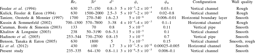
A list of experimental studies addressing gas–solid wall-bounded flows. When not explicitly reported in the referenced papers, the parameters are calculated using information therein.

In this scenario, the importance of well-controlled laboratory experiments is paramount to reach a predictive understanding of these regimes, and to inform and validate numerical models. Unfortunately, similar studies are rare in the literature and cover limited portions of the parameter space. Several past experiments considered particle–laden water flows with
 $\unicode[STIX]{x1D70C}_{p}/\unicode[STIX]{x1D70C}_{f}=\mathit{O}(1)$
and particle diameters of several wall units (Kaftori et al.
Reference Kaftori, Hetsroni and Banerjee1995a
,Reference Kaftori, Hetsroni and Banerjee
b
; Niño & Garcia Reference Niño and Garcia1996; Kiger & Pan Reference Kiger and Pan2002; Righetti & Romano Reference Righetti and Romano2004; Rabencov, Arca & van Hout Reference Rabencov, Arca and van Hout2014; Oliveira, van der Geld & Kuerten Reference Oliveira, van der Geld and Kuerten2017; Shokri et al.
Reference Shokri, Ghaemi, Nobes and Sanders2017). These conditions are relevant to sediment transport and pipelines, but not to other important applications such as dust and particulate transport in air. For gas–solid suspensions, a non-exhaustive list of previous experiments and their relevant physical parameters is provided in table 1. Currently, the main reference is still represented by the vertical channel flow measurements by Eaton and co-workers. In particular, Fessler et al. (Reference Fessler, Kulick and Eaton1994) and Kulick et al. (Reference Kulick, Fessler and Eaton1994) provided seminal insight into preferential concentration and turbulence modulation for a variety of regimes. However, Benson et al. (Reference Benson, Tanaka and Eaton2005) showed that their apparatus presented substantial wall roughness due to particle deposition on the walls, which according to Vreman (Reference Vreman2015) partly explained the disagreement with simulations. Benson et al. (Reference Benson, Tanaka and Eaton2005) repeated the measurements with a smooth test section, only focusing on the most inertial particles that did not display turbophoresis. Taniere et al. (Reference Taniere, Oesterle and Monnier1997) investigated a particle–laden boundary layer in a horizontal wind tunnel, focusing on particles with
 $St^{+}>270$
. As in all horizontal flow configurations, the particle concentration profile was strongly impacted by gravity. Kussin & Sommerfeld (Reference Kussin and Sommerfeld2002) measured particle motion and concentration as well as turbulence modulation in a horizontal channel flow with rough walls. Their particles were highly inertial and could not display turbophoresis or turbulence-induced clustering. Caraman et al. (Reference Caraman, Borée and Simonin2003) considered a vertical particle–laden pipe flow in a regime where turbophoresis is expected, and carried out a detailed analysis of the moments of the particle velocity. Still, comparison with simulations was hampered by the measurement station being downstream of the pipe exit, the lack of concentration profiles and possible wall roughness (Vreman Reference Vreman2007). Khalitov & Longmire (Reference Khalitov and Longmire2003) conducted measurements in a vertical channel flow laden with glass spheres of various sizes, covering a range of Stokes numbers for which turbophoresis is expected. They documented both particle–particle and gas–particle velocity correlations in the streamwise and spanwise directions, but not the concentration profiles. Hadinoto et al. (Reference Hadinoto, Jones, Yurteri and Curtis2005) considered a vertical pipe flow laden with glass beads that were too inertial to segregate at the wall. Li et al. (Reference Li, Wang, Liu, Chen and Zheng2012) imaged inertial particles at
 $St^{+}\approx 100$
in a range of concentrations where two-way coupling effects are expected to be weak. Because their channel was horizontal and they only reported data near the bottom wall, possible turbophoresis was not distinguishable from gravitational settling.
Overall, there is a clear lack of laboratory observations of wall-bounded gas–solid flows in regimes where preferential concentration and turbophoresis are at play. In particular, little is known on the changes occurring when varying the loading across what is considered the boundary between one-way and two-way coupling. Liquid–solid flow studies cannot compensate for these deficiencies in the literature, as the momentum coupling is heavily affected by the density ratio. Importantly, concentration profiles are seldom reported, and therefore near-wall segregation (clearly evident in simulations) has not been fully documented. The seminal studies usually cited as experimental evidence of this phenomenon (e.g. Kaftori et al. Reference Kaftori, Hetsroni and Banerjee1995a ,Reference Kaftori, Hetsroni and Banerjee b ) were carried out in horizontal flumes where gravitational effects may be important. In order to bridge such knowledge gap, the present study experimentally investigates the transport of small solid particles in turbulent air flowing downward in a smooth-wall vertical channel. We focus on regimes (summarized in table 1) for which significant clustering and turbophoresis are expected, and use planar imaging to analyse the particle behaviour for different levels of mass loading. The paper is organized as follows: in § 2 we describe the laboratory facility and the methods used to conduct the experiments and analyse the data; in § 3 we present the wall-normal profiles of particle concentration and velocities, and the spatial fields along wall-parallel planes at the channel core and near the wall; conclusions and an outlook for further research are provided in § 4.
2 Experimental method
2.1 Experimental facility and parameters
Experiments are conducted in a vertical recirculating wind tunnel depicted in figure 1, featuring a 1.9 m long rectangular channel with a 0.24 m by 0.03 m cross-section. A 1.5 kW centrifugal blower (Atlantic Blowers) controlled by a frequency converter drives air downwards, and the flow rate is continuously monitored via a Venturi flowmeter. Before the air enters the channel, size-selected glass beads (Mo-Sci Corp.) with a density of
 $2500~\text{kg}~\text{m}^{-3}$
and diameter of
 $50\pm 6~\unicode[STIX]{x03BC}\text{m}$
(mean
 $\pm$
standard deviation measured by optical microscopy over
 $\mathit{O}(10^{4})$
samples) are injected into the flow through a precision screw-feeder (Vibra Screw Inc.). This corresponds to a ratio of channel width to particle diameter of
 $2h/d_{p}=600$
. A flow-conditioning section consisting of four screens and three honeycombs is placed at the channel inlet to disperse the particles uniformly. The measurement station consists of a 0.3 m long, fully transparent acrylic section that follows a 1.6 m long development section. The latter has a through-flow time 25–40 times larger than the particle response time, depending on the air-flow regime. Integration of the particle equation of motion with the Schiller and Neumann correction (Clift, Grace & Weber Reference Clift, Grace and Weber2005) indicates that the particles reach their terminal velocity in about half the time it takes them to reach the test section. The particles exhausted from the channel are collected in a 109-litre settling chamber, allowing for the run times needed to achieve well-converged statistics without particles being ingested into the blower. Electrostatic dissipative acrylic (SciCron Technologies) is used to build the optical test section, and the channel is provided with static discharge wires grounded to structural supports. This prevents the particles from accumulating upon impaction and building up unwanted roughness, an effect that has impacted past experiments (Benson et al.
Reference Benson, Tanaka and Eaton2005). This point is demonstrated and elaborated upon in appendix A.
A schematic diagram of the particle–laden channel flow facility and its main elements.

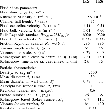
The fluid and particle parameters for the investigated cases are listed in table 2. Two flow rates are considered, associated with friction Reynolds numbers
 $Re_{\unicode[STIX]{x1D70F}}=235$
and 335, respectively. The particle Reynolds number, defined with the still-air terminal velocity of the particles
 $V_{t}=\unicode[STIX]{x1D70F}_{p}g=0.17~\text{m}~\text{s}^{-1}$
as a representative relative velocity with respect to the fluid, is
 $Re_{p}<1$
(here
 $g$
is the gravitational acceleration). Using the particle root mean square (r.m.s.) of the particle velocity fluctuations as a velocity scale leads to higher values, but still within
 $Re_{p}=\mathit{O}(1)$
, suggesting that particle wakes negligibly affect the flow. The Froude number, defined as the ratio of the centreline fluid velocity to the still-air settling velocity, satisfies the condition
 $Fr\gg 1$
. It has been argued that this warrants a negligible influence of gravity (see the boundary layer study of Sardina et al. (Reference Sardina, Schlatter, Picano, Casciola, Brandt and Henningson2012b
), where the free-stream velocity is used to define
 $Fr$
). However, this condition is not strictly applicable to the near-wall region where the fluid velocity vanishes. Moreover, for particle–turbulence interaction the relevant velocity scale is arguably the fluid r.m.s. fluctuation, which at the channel centreline is of the same order of magnitude as the still-air settling velocity. Indeed, recent measurements in a vertical pipe from Oliveira et al. (Reference Oliveira, van der Geld and Kuerten2017) at
 $Fr>10$
show large differences in particle behaviour between downward and upward flow. Therefore, we will not generalize the present findings to other channel orientations, as gravity may play a significant role in this regime (as also discussed in § 3).
Fluid and particle parameters for the investigated cases. Parameter
 $\unicode[STIX]{x1D702}_{c}$
is calculated using the relation
 $\unicode[STIX]{x1D702}_{c}=\unicode[STIX]{x1D706}_{\unicode[STIX]{x1D708}}(\unicode[STIX]{x1D705}Re_{\unicode[STIX]{x1D70F}})^{1/4}$
(Pope Reference Pope2000).

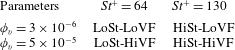
Cases studied in this experiment and respective notation.

The regimes
 $Re_{\unicode[STIX]{x1D70F}}=235$
and 335 are associated with different fluid time scales, resulting in two different Stokes number cases referred to as LoSt and HiSt, respectively. The change in Reynolds number, while not inconsequential, is expected to have a lesser impact over the considered range compared to the variation in
 $St$
. The range of
 $St^{+}$
and
 $St_{\unicode[STIX]{x1D702}}$
(the latter being defined with the Kolmogorov time scale at the channel centreline in the unladen flow) suggests significant turbophoresis and preferential concentration. For each Stokes number, two sets of measurements are carried out by changing the screw size in the particle feeder, resulting in volume fractions
 $\unicode[STIX]{x1D719}_{v}=3\times 10^{-6}$
(for a mass loading
 $\unicode[STIX]{x1D719}_{m}=0.6\,\%$
) and
 $5\times 10^{-5}$
(
 $\unicode[STIX]{x1D719}_{m}=10\,\%$
), referred to as LoVF and HiVF, respectively. These correspond to global concentrations
 $C_{0}=46$
and
 $880~\text{particles}~\text{cm}^{-3}$
, respectively. The four-case matrix is summarized in table 3. The fluid-phase parameters in table 2 are based on the unladen flow, characterized by particle image velocimetry as described in the following. While the mass loading for the LoVF cases is not expected to produce sizeable changes in the fluid flow, in the HiVF cases the turbulence is likely to be impacted (Kulick et al.
Reference Kulick, Fessler and Eaton1994), and therefore the listed values of the flow properties should be regarded as estimates.
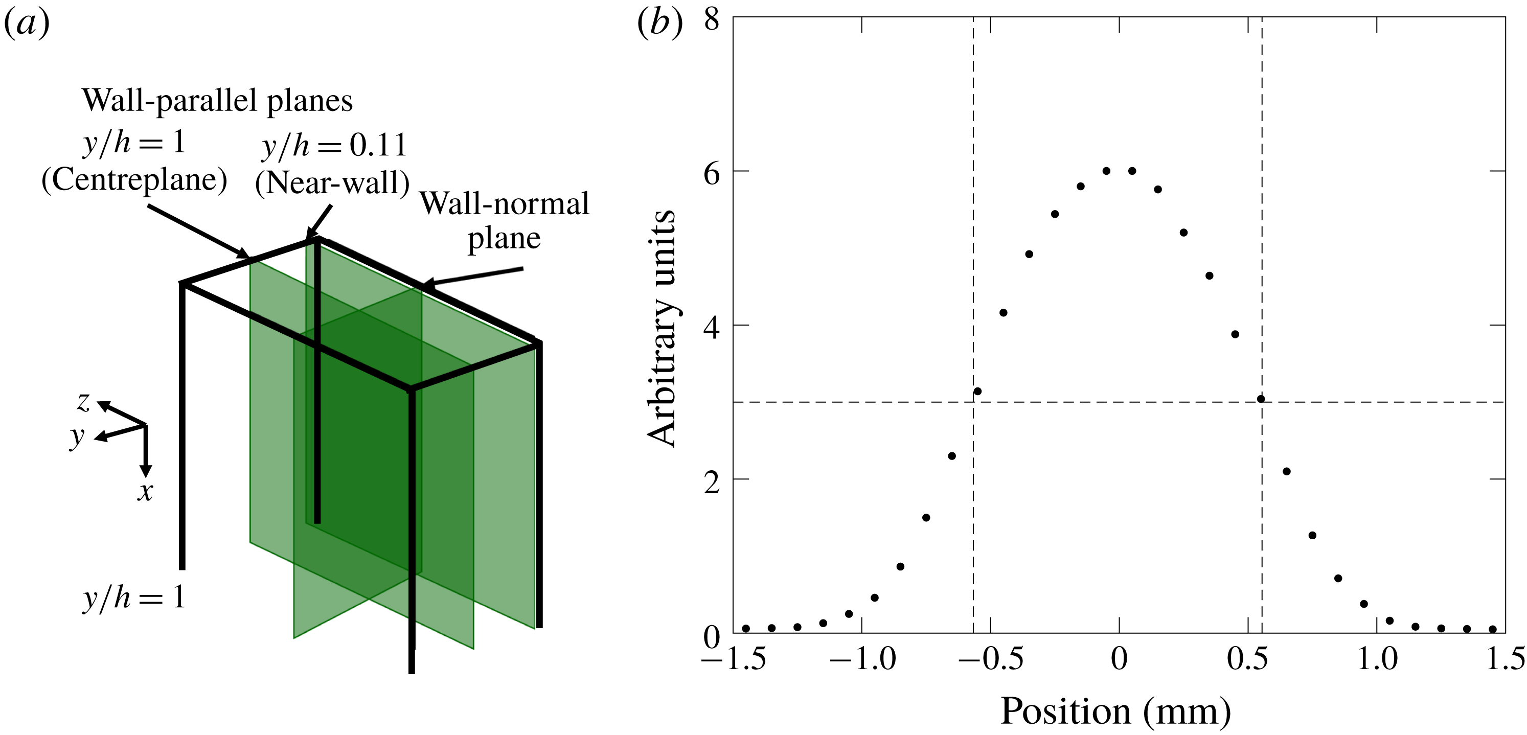
(a) Main imaging planes investigated in the present study. (b) Light intensity profile as measured by a photodiode to estimate the laser sheet thickness. The dashed lines mark the full width at half maximum.

The coefficient of restitution,
 $e$
, for particle–wall collisions is measured in a separate experiment. Here
 $e$
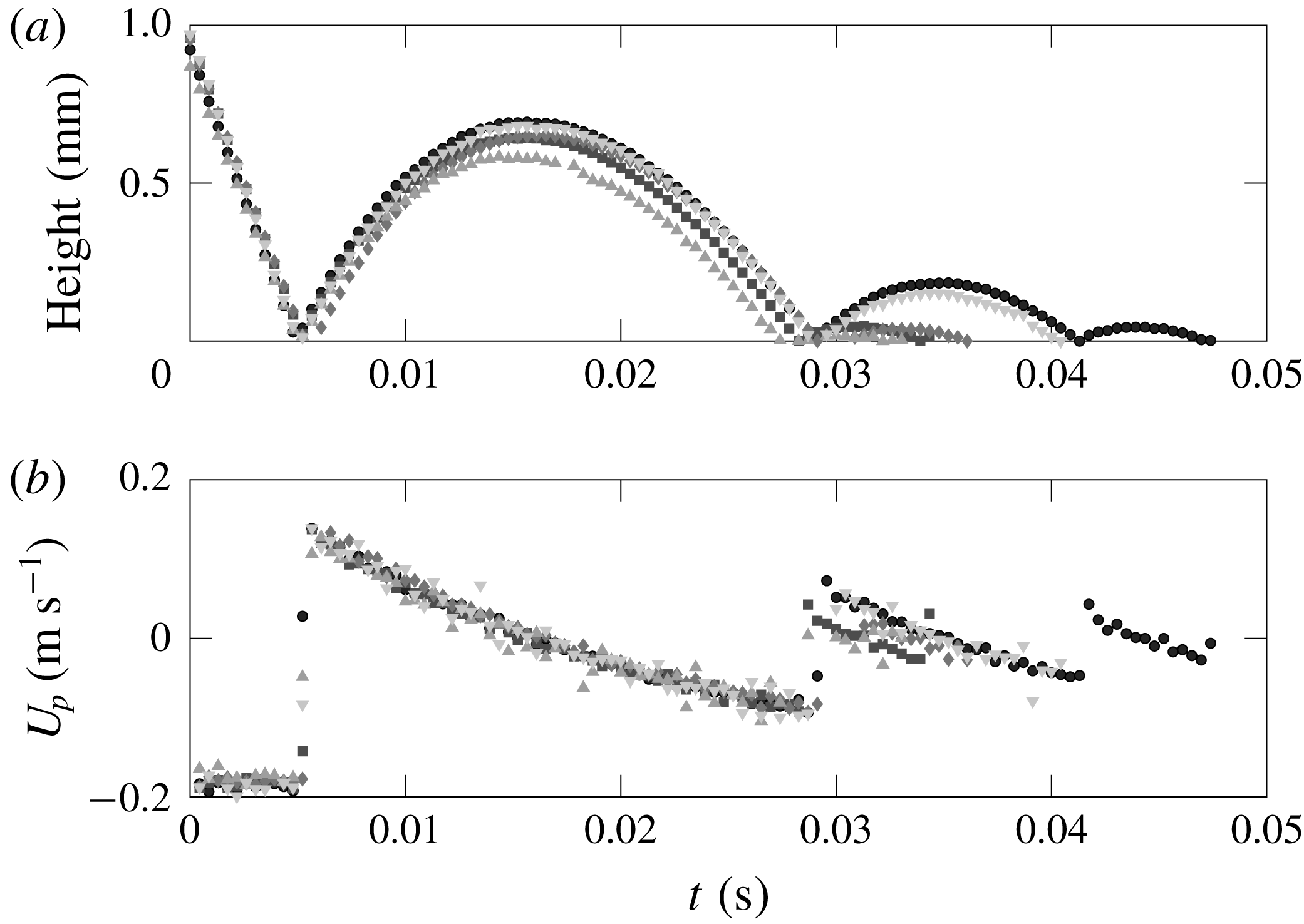
is defined as the ratio of the wall-normal particle velocity just after and just before the collision; details of the experimental measurements are elaborated upon in appendix B. It is known that the value of
 $e$
is dependent on the particle Reynolds number and Stokes number based on the particle velocity relative to the fluid (Gondret, Lance & Petit Reference Gondret, Lance and Petit2002). However, the terminal velocity happens to be of the order of the r.m.s. wall-normal velocity of the particles in the vicinity of the wall (
 $0.02U_{c}$
–
 $0.05U_{c}$
, where
 $U_{c}$
is the centreline velocity), as will be shown later. Thus, the quoted restitution coefficient is relevant to the particle–laden flow condition. Still, the actual collision velocity in the channel flow experiment is expected to have significant scatter; possible consequences of such variance are discussed in § 4.
2.2 Measurement methods
The imaging system consists of a double-pulsed Nd:YAG laser (
 $30~\text{mJ}~\text{pulse}^{-1}$
, New Wave Instruments) and a
 $1376~\text{pixel}\times 1040~\text{pixel}$
CCD camera (Sensicam, PCO Instruments) operated at 5 Hz and synchronized to the laser via a delay generator (BNC-5500, Berkeley Nucleonics). Planar measurements are obtained by shaping the laser beam into a sheet via an optical module combining cylindrical and spherical lenses. For all cases, the measurement locations include a wall-normal plane that contains the channel centreline. We denote with
 $x$
,
 $y$
and
 $z$
the streamwise, wall-normal and spanwise directions, the channel walls being located at
 $y=0$
and
 $y=2h$
. For the HiVF cases, several wall-parallel planes are also imaged and compared, one at the centreline (
 $y=h$
) and one in the near-wall region (
 $y=0.11h$
); see figure 2(a). An additional wall-parallel plane (not shown in figure 2
a) is imaged at
 $y=0.2h$
for comparisons with wall-normal profiles. Spatial calibration and plane location are performed by imaging a target plate mounted on a micrometric traverse, inserted in the channel from the opening at the outflow end. The laser sheet thickness is evaluated using a photodiode (Thorlabs Inc.) coupled with a neutral density filter (CW Optics) and mounted on a traverse. The full width at half maximum is approximately 1.1 mm (figure 2
b).
The unladen (single-phase) case is characterized using two-component, two-dimensional particle image velocimetry along the wall-normal symmetry plane. The flow is seeded with DEHS oil atomized by a Laskin nozzle into
 $1{-}2~\unicode[STIX]{x03BC}\text{m}$
droplets that faithfully follow the flow, their viscous Stokes number being
 $\mathit{O}(10^{-2})$
. For those measurements, the CCD camera mounts a 200 mm Micro-Nikkor lens at f
 $/$
5.6 to obtain a
 $13.3\times 10.1~\text{mm}^{2}$
field of view. The full channel height is covered by stitching together four slightly overlapping windows. The pulse delay is set to
 $10$
and
 $15~\unicode[STIX]{x03BC}\text{s}$
for the higher and lower flow rate, respectively, keeping the typical tracer displacement to about 8 pixels. Image pairs are processed via a multi-pass cross-correlation algorithm, with a final interrogation window of
 $32~\text{pixels}\times 32~\text{pixels}$
and 50 % overlap. Flow statistics are obtained by ensemble-averaging over 2000 uncorrelated realizations as well as in the homogeneous streamwise direction. The fully developed nature of the flow at the measurement station is confirmed by comparing profiles across the imaging window, with no appreciable changes for statistics up to second order.
In the particle–laden cases, the inertial particle position and velocity are characterized by particle tracking velocimetry using an in-house code developed based on the cross-correlation methods described in Hassan et al. (Reference Hassan, Blanchat, Seeley and Canaan1992) and Ohmi & Li (Reference Ohmi and Li2000). Further details of the algorithm can be found in Petersen, Baker & Coletti (Reference Petersen, Baker and Coletti2019). For the measurements along the wall-normal plane, the CCD camera mounts a 105 mm Micro-Nikkor lens at f
 $/$
16, providing an imaging magnification of
 $36.1~\text{pixels}~\text{mm}^{-1}$
for a
 $34.3\times 25.9~\text{mm}^{2}$
field of view encompassing the full channel height. The particle-per-pixel density is
 $4.0\times 10^{-5}$
for the LoVF cases and
 $6.9\times 10^{-4}$
for the HiVF cases. Along the wall-parallel planes, an aperture of f
 $/$
4 is used, providing an imaging magnification of
 $19.0~\text{pixels}~\text{mm}^{-1}$
for a
 $55\times 70~\text{mm}^{2}$
window at the spanwise centre of the channel. The particle-per-pixel density is
 $1.8\times 10^{-3}$
for the centreplane and
 $3.9\times 10^{-3}$
for the near-wall plane. The particle images are about 3 pixels, whose centroid is retrieved with an accuracy of approximately
 $\pm 0.1$
pixels, as confirmed by tests on synthetic images. The pulse delay ranges between
 $70$
and
 $100~\unicode[STIX]{x03BC}\text{s}$
depending on the cases and imaging locations, with typical particle displacements of 15–20 pixels. A pre-processing thresholding routine is applied to eliminate out-of-focus particles. The in-focus particles are tracked between image pairs using the relaxation method described by Baek & Lee (Reference Baek and Lee1996). The local concentration is measured along the wall-normal plane by counting the number of particle centroids detected. This approach was used for inertial particles in air (Yang & Shy Reference Yang and Shy2005; Sahu, Hardalupas & Taylor Reference Sahu, Hardalupas and Taylor2014, Reference Sahu, Hardalupas and Taylor2016) and in water (Kiger & Pan Reference Kiger and Pan2002). Knowles & Kiger (Reference Knowles and Kiger2012) showed that, in water, laser-based measurements of particle concentration can be misestimated by as much as 30 %; however, they considered volume fractions one order of magnitude higher than the present case. Even at the higher loading investigated here, the average interparticle distance is
 ${\sim}1~\text{mm}$
, which is much larger than the particle image. Due to clustering, the instantaneous local concentration can be higher, and some particles may go undetected. However, intense clustering usually pertains to a limited fraction of the particle set (Baker et al.
Reference Baker, Frankel, Mani and Coletti2017); here the regions where such bias may be more significant are near the wall, due to turbophoresis. Still, the volume fraction evaluated from the particle count along the wall-normal plane (assuming a 1.1 mm thick imaging volume) agrees within 12–15 % with the value obtained by weighing the particles accumulated in the settling chamber during a given run time, lending confidence to the approach. Concentration and velocity statistics are based on ensemble-averaging over 2000 uncorrelated realizations (collected over four runs of 500 realizations each) as well as over the streamwise direction. The streamwise homogeneity of the particle statistics is discussed in § 3.1.3. All statistics are verified to be steady state during each run, with excellent repeatability in each run (within variations of the order of the statistical uncertainty). It is noted that simultaneous fluid-phase measurements are not acquired in this experiment. This is due to the relatively high image concentration of the inertial particles, especially near the wall, reducing the signal from fluid tracers. The feasibility of obtaining simultaneous fluid measurements is discussed in § 4.
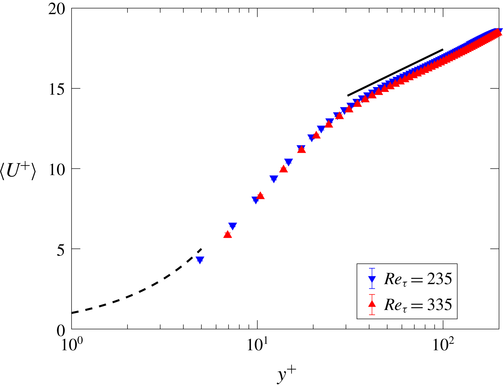
The mean velocity profile shown in logarithmic scale for
 $Re_{\unicode[STIX]{x1D70F}}=235$
and 335. The dashed black line represents the expected fluid velocity profile in the viscous sublayer (
 $y^{+}<5$
). The solid black line indicates the log-law slope (
 $K=0.41$
,
 $B=5.2$
, shifted up 1 unit in diagram for illustration) used to determine the friction Reynolds number from
 $y^{+}=30$
to 100.

3 Results
Throughout this section,
 $\langle U\rangle$
and
 $\langle V\rangle$
denote streamwise and wall-normal components of the mean velocity. Components
 $u$
and
 $v$
are the corresponding fluctuating components, whose r.m.s. are denoted as
 $U_{rms}$
and
 $V_{rms}$
, respectively. Error bars in the plots represent statistical uncertainties based on 95 % confidence levels and using the random uncertainty of the dataset (Bendat & Piersol Reference Bendat and Piersol2011). When the wall-normal profiles are shown over half of the channel height, the symmetry of the results along the centreline is within the statistical uncertainty.
3.1 Wall-normal measurements
3.1.1 Unladen air flow
As a baseline, we first present the wall-normal profiles for the unladen fluid velocity. These are plotted in inner units in figure 3, showing the expected logarithmic behaviour above
 $y^{+}\sim 30$
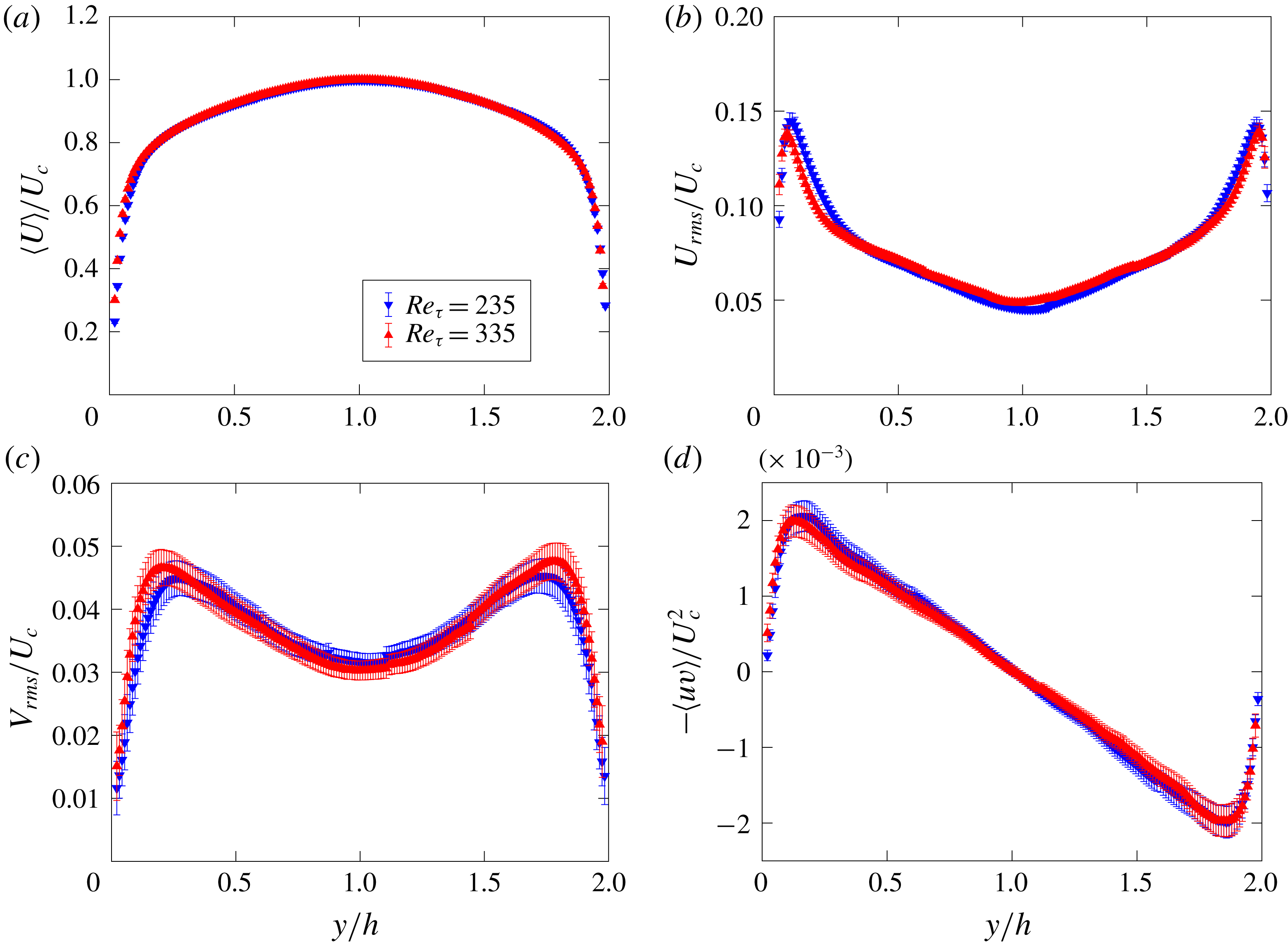
. This is used to determine the friction velocity using a Clauser chart method (Clauser Reference Clauser1956; Wei, Schmidt & McMurtry Reference Wei, Schmidt and McMurtry2005). The profiles for the mean velocity, streamwise and wall-normal r.m.s. fluctuation and Reynolds shear stress are plotted in figure 4 in outer units, i.e. normalized by the channel half-height and the centreline velocity. The agreement with DNS of spanwise-periodic channels at comparable Reynolds numbers (e.g. Moser, Kim & Mansour Reference Moser, Kim and Mansour1999) suggests that the flow in the central part of the channel is not significantly impacted by the finite width of the cross-section.
Wall-normal profiles for the unladen flow at both considered Reynolds numbers, normalized in outer units: (a) mean velocity; (b) streamwise r.m.s. velocity fluctuation; (c) wall-normal r.m.s. velocity fluctuation; (d) Reynolds shear stress.

3.1.2 Particle concentration
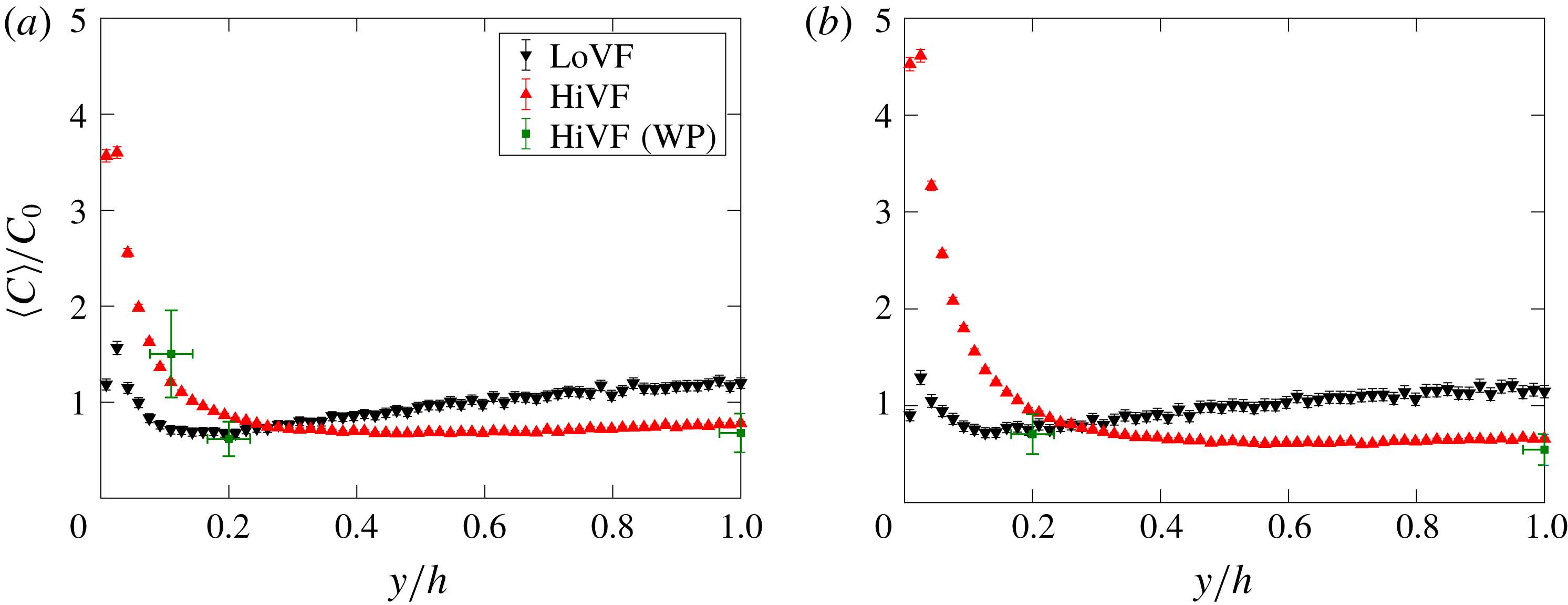
Figure 5 displays the mean profiles of normalized particle concentration
 $C/C_{0}$
for the four particle–laden cases. Here and in the following wall-normal profile plots, data points in the profiles are plotted at the
 $y/h$
location at the centre of the respective wall-normal bin, each bin having a width of 0.25 mm (about 9 pixels). Data points measured for the HiVF cases along wall-parallel planes are also shown and found to agree closely with the wall-normal imaging results. Both LoVF and HiVF cases display a peak of concentration in the near-wall region, confirming that turbophoresis is active in the present regime. However, in the more dilute cases the peak is mild, and away from the wall the concentration gradually increases towards another local maximum at the centreline. On the other hand, the higher-loading cases display a much stronger peak of concentration near the wall, and the profile is essentially flat in the core region. The peaks appear to be at a finite standoff distance from the wall, which is however hard to quantify precisely.
As mentioned in the Introduction, previous measurements of near-wall segregation in similar regimes are lacking, and a comparison with past numerical simulations is in order. We refer to point-particle DNS studies, which are free from issues associated with turbulence modelling. Among those, several one-way-coupled simulations yielded near-wall concentration peaks two or more orders of magnitude above the channel mean, and mostly contained within the viscous sublayer (Marchioli & Soldati Reference Marchioli and Soldati2002; Marchioli et al.
Reference Marchioli, Soldati, Kuerten, Arcen, Taniere, Goldensoph, Squires, Cargnelutti and Portela2008; Sardina et al.
Reference Sardina, Schlatter, Brandt, Picano and Casciola2012a
; Bernardini Reference Bernardini2014). Those results, while insightful, are influenced by the fact that point particles can amass to arbitrary densities. In two-way-coupled simulations, the momentum back-reaction from the particles reduced the near-wall segregation, as did the interparticle collisions; see Li et al. (Reference Li, McLaughlin, Kontomaris and Portela2001), Vreman (Reference Vreman2007) and Nasr et al. (Reference Nasr, Ahmadi and McLaughlin2009). Those authors did show concentrations reaching a minimum adjacent to the near-wall peak and increasing up to a centreline maximum, similarly to our LoVF profiles. However, they found that such reduction of the near-wall peak (and the simultaneous appearance of a centreline maximum) occurred for increasing mass loading, in contrast with the present results. On the other hand, the concentration profiles we observe for LoVF are consistent with the argument of Young & Leeming (Reference Young and Leeming1997) that turbophoresis is driven by the gradient of fluid
 $V_{rms}$
(figure 4
c). The concentration is maximized in correspondence to the concentration minimum, decays steeply towards the wall and more mildly towards the centreline, following approximately the same trend as the wall-normal gradient of
 $V_{rms}$
. We remark that the centreline concentration maximum was observed in several, but not all, one-way-coupled simulations, and was found to depend on the flow orientation: for example, Nilsen et al. (Reference Nilsen, Andersson and Zhao2013) found it for downward and no-gravity flow, but not for upward flow.
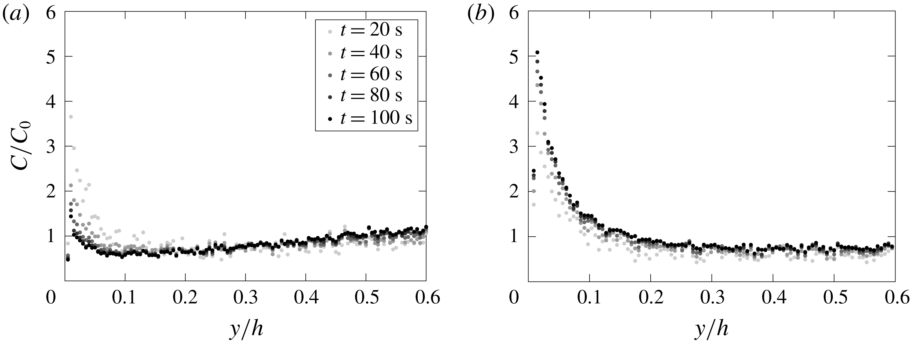
Mean particle concentration profiles normalized by the global concentration for (a) LoSt cases and (b) HiSt cases. Here and in the following plots, WP indicates data points from wall-parallel measurements, with the horizontal error bars indicating uncertainty on laser sheet position.

3.1.3 Particle velocity
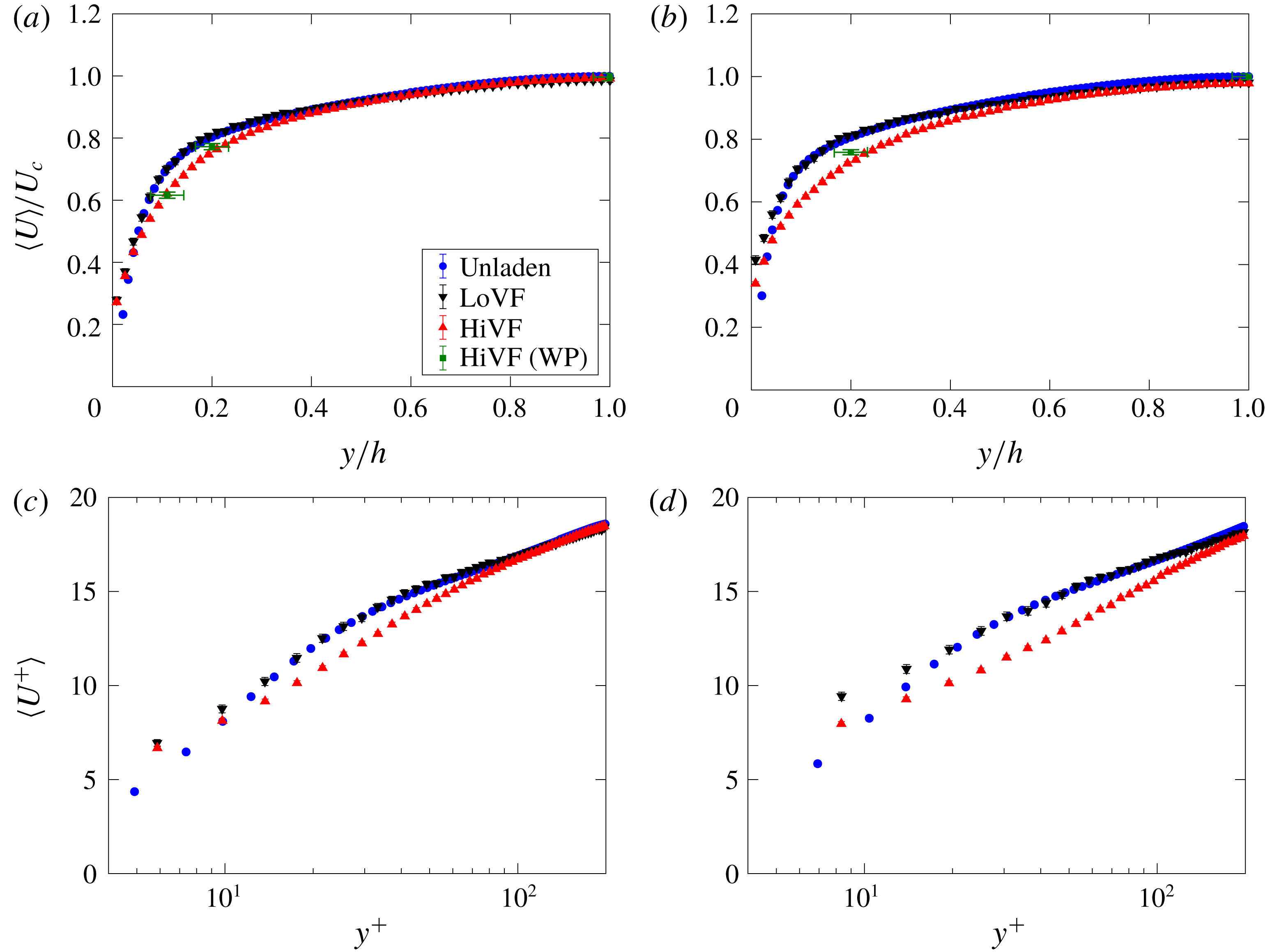
Figure 6 displays mean velocity profiles compared to the unladen air velocity. The data are presented both in outer (figure 6
a,b) and inner (figure 6
c,d) units, normalizing by the unladen velocity scales. In the viscous and buffer layer, the particles travel faster than the unladen air. This is a consequence of fast-moving particles retaining part of their momentum when transported towards the wall by turbulent fluctuations, without being constrained by the no-slip boundary condition. Such behaviour was already highlighted by Kulick et al. (Reference Kulick, Fessler and Eaton1994) and in several later experimental and numerical studies (e.g. Taniere et al.
Reference Taniere, Oesterle and Monnier1997; Rouson & Eaton Reference Rouson and Eaton2001; Vreman Reference Vreman2007; Li et al.
Reference Li, Wang, Liu, Chen and Zheng2012). Righetti & Romano (Reference Righetti and Romano2004) explicitly commented on an effective slip boundary condition for the particle field. Further away from the wall, in the LoVF cases the particles travel at approximately the same speed as the unladen air, while in the HiVF cases they lag in the logarithmic and buffer layers, recovering to the unladen air velocity in the channel core. A decrease of mean velocity with increasing mass loading was also reported by Kulick et al. (Reference Kulick, Fessler and Eaton1994), although for higher
 $St^{+}$
. In that case the lag was visible up to the centreline, but this was likely due to the wall roughness (Benson et al.
Reference Benson, Tanaka and Eaton2005). In general, we observe less flat velocity profiles than in previous experiments; see, for example, Kulick et al. (Reference Kulick, Fessler and Eaton1994), Paris (Reference Paris2001), Caraman et al. (Reference Caraman, Borée and Simonin2003) and Benson et al. (Reference Benson, Tanaka and Eaton2005). Vreman (Reference Vreman2015) argued that those were again influenced by some wall roughness that enhanced the wall-normal particle velocity fluctuations and in turn flattened the mean velocity profiles.
Profiles of mean streamwise particle velocity for (a,c) LoSt and (b,d) HiSt cases, normalized in outer units (a,b) and inner units (c,d). Unladen fluid profiles are plotted for comparison.

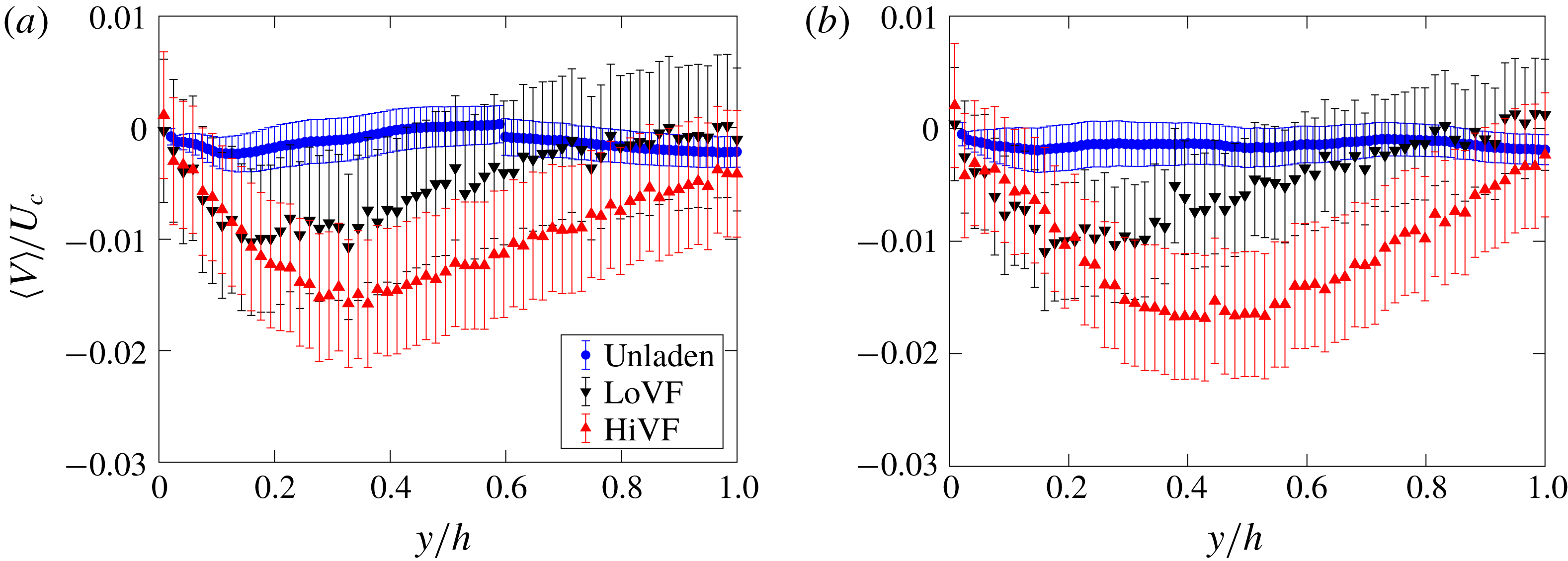
Figure 7 displays profiles of mean wall-normal particle velocity. In a fully developed state, this should be identically zero. This is the case (within error bounds) for the unladen fluid, while the particles do show some residual drift towards the wall. This is likely caused by turbophoresis; the effect is exemplified in the LoVF case where the peak at
 $y/h\sim 0.2$
approximately corresponds to the maximum of unladen fluid
 $V_{rms}$
and to the minimum of particle concentration, consistent with the theory of Young & Leeming (Reference Young and Leeming1997) (see also Capecelatro, Desjardins & Fox Reference Capecelatro, Desjardins and Fox2016). Numerical simulations at similar
 $St^{+}$
indicated that the turbophoretic drift continues to modify the particle field during
 $\mathit{O}(10^{4})$
viscous time scales, which over the considered range of
 $Re_{\unicode[STIX]{x1D70F}}$
corresponds to
 $\mathit{O}(10^{3})$
channel heights (Marchioli et al.
Reference Marchioli, Soldati, Kuerten, Arcen, Taniere, Goldensoph, Squires, Cargnelutti and Portela2008; Sardina et al.
Reference Sardina, Schlatter, Brandt, Picano and Casciola2012a
; Bernardini Reference Bernardini2014). While these estimates are influenced by the one-way coupled nature of the modelling, they clearly indicate that the particle field requires a much greater development length than the sole hydrodynamics. However, we also remark that the observed wall-normal mean velocities are about 1 % of the streamwise velocity, and smaller than the r.m.s. fluctuation in the same direction (reported below). Moreover, all statistics show no visible trend over the imaging windows (about
 $1.7h$
and
 $3.7h$
in the streamwise direction for the wall-normal and wall-parallel measurements, respectively). Thus, also considering that the particles are expected to have reached terminal velocity much before entering the imaging section, the influence of the partial streamwise development is unlikely to qualitatively impact the reported trends.
Profiles of mean wall-normal particle velocity for (a) LoSt and (b) HiSt cases. Unladen fluid profiles are plotted for comparison.

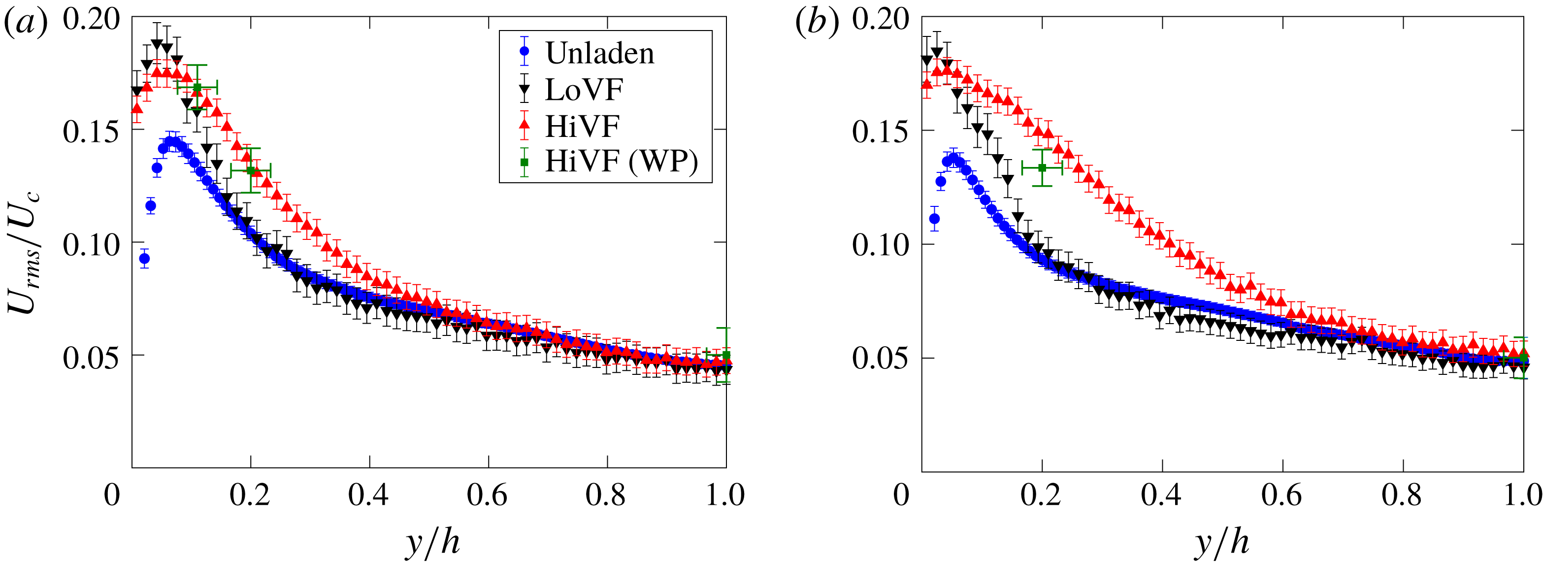
Profiles of r.m.s. streamwise particle velocity for (a) LoSt and (b) HiSt cases. Unladen fluid profiles are plotted for comparison.

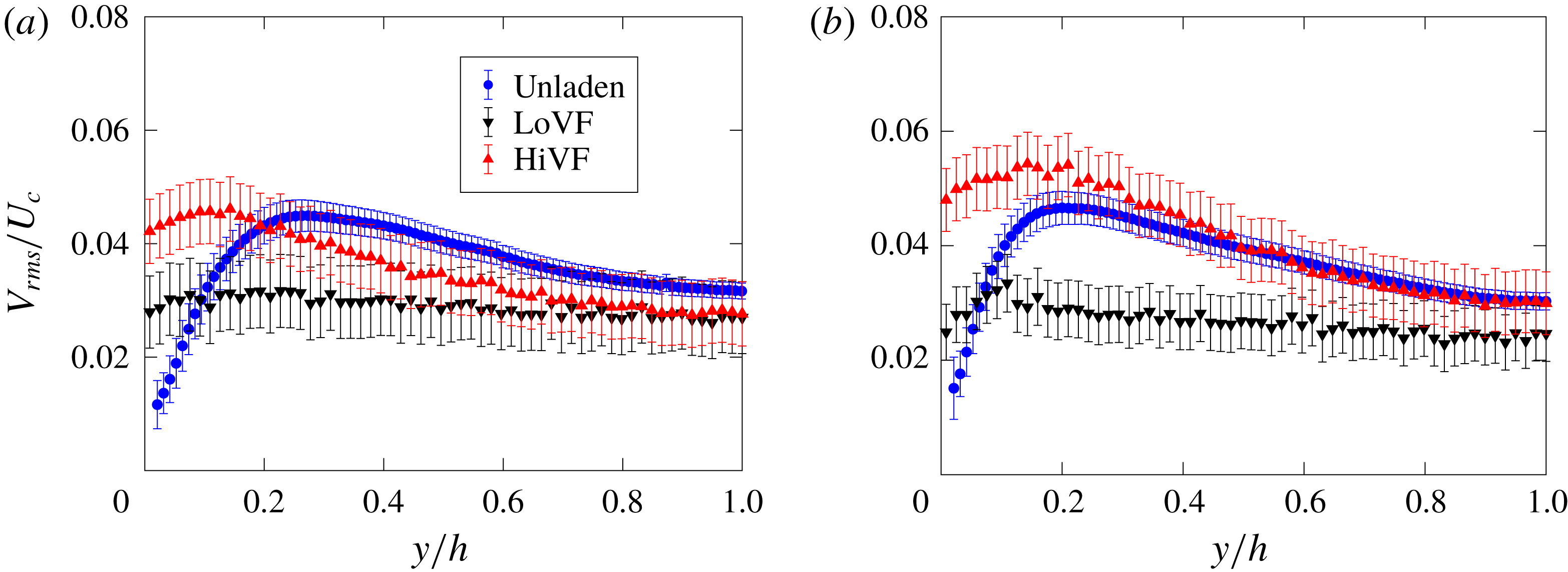
Profiles of r.m.s. wall-normal particle velocity for (a) LoSt and (b) HiSt cases. Unladen fluid profiles are plotted for comparison.

The r.m.s. streamwise fluctuations of the particle velocity are plotted in figure 8. The LoVF cases display profiles similar to those of the unladen flow in the channel core, and significantly more intense fluctuations (up to 20 % higher than the fluid) in the near-wall region, with little differences between LoSt and HiSt. Previous studies have found particles with velocity fluctuations stronger than the carrier fluid in several configurations, including particle–laden jets and homogeneous turbulence (e.g. Hardalupas, Taylor & Whitelaw Reference Hardalupas, Taylor and Whitelaw1989; Petersen et al.
Reference Petersen, Baker and Coletti2019). Specifically in channel flows, the observed trend agrees with one-way coupled simulations as reported by Marchioli et al. (Reference Marchioli, Soldati, Kuerten, Arcen, Taniere, Goldensoph, Squires, Cargnelutti and Portela2008) and Nasr et al. (Reference Nasr, Ahmadi and McLaughlin2009) for lower but still turbophoretic Stokes numbers. Following Taniere et al. (Reference Taniere, Oesterle and Monnier1997), the increase in r.m.s. velocities may be interpreted as a consequence of the spread in momentum of particles with different history: the ones arriving to a near-wall interrogation window from more distant locations retain some of their relatively high speed due to inertia; while those coming from a rebound on the wall have lost some of their kinetic energy in the collision. Remarkably, the HiVF cases show a significant increase of particle velocity fluctuations even at
 $y/h\sim 0.4$
, which is even more dramatic for HiSt. The near-wall peak is about the same as in LoVF, but the cross-section-average r.m.s. fluctuation is substantially augmented for the higher loading. This is in contrast with past two-way and four-way coupled point-particle DNS: considering mass loadings higher than but comparable to the current HiVF cases, Li et al. (Reference Li, McLaughlin, Kontomaris and Portela2001), Vreman (Reference Vreman2007) and Nasr et al. (Reference Nasr, Ahmadi and McLaughlin2009) found a decrease in streamwise r.m.s. fluctuations (although the trend with increasing
 $\unicode[STIX]{x1D719}_{v}$
reported by Vreman was locally not monotonic at high loadings).
Figure 9 shows profiles of the wall-normal r.m.s. fluctuations of the particle velocities. For LoVF, the particle
 $V_{rms}$
is lower than the unladen fluid
 $V_{rms}$
in the channel core, but it remains fairly flat across the channel and largely exceeds the unladen fluid levels for
 $y/h<0.1$
. The effect of
 $St^{+}$
in the considered range is minor. Moreover, while the fluctuation level decreases approaching the wall, it does not appear to vanish. This is in contrast with one-way coupled simulations where the particle
 $V_{rms}$
is consistently lower than the fluid
 $V_{rms}$
(thus vanishing at the wall; Marchioli et al.
Reference Marchioli, Soldati, Kuerten, Arcen, Taniere, Goldensoph, Squires, Cargnelutti and Portela2008), but is consistent with previous experiments with particles of similar
 $St^{+}$
(Li et al.
Reference Li, Wang, Liu, Chen and Zheng2012). The approximately even redistribution of the lateral kinetic energy across the channel cross-section may partly be due to particle inertia, and partly to collisions with the wall (interparticle collision being relatively unlikely at the lower volume fraction). For HiVF,
 $V_{rms}$
increases more significantly approaching the wall, and the tendency is stronger for HiSt. This behaviour is similar as for
 $U_{rms}$
, and indicates again that the particle–fluid dynamics has been altered: by the modification of the underlying turbulent flow and/or by the increase in particle–particle/wall–particle collisions.
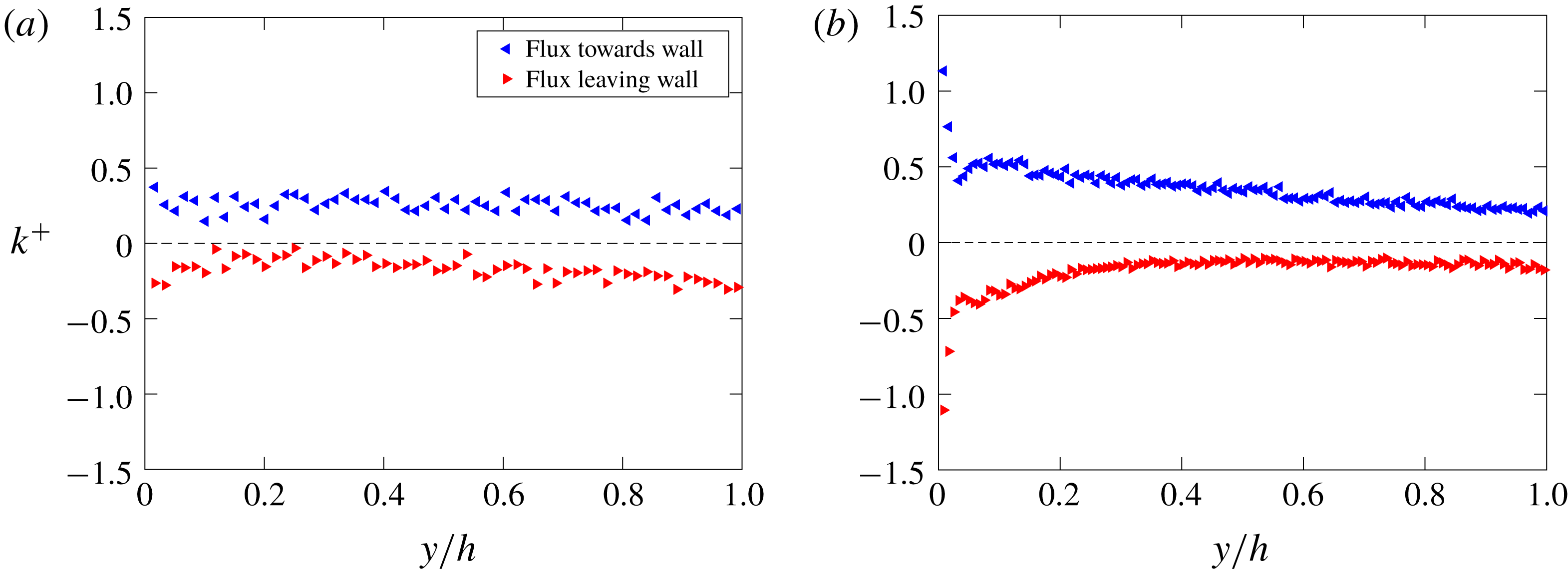
The wall-normal velocity is tightly related to the particle flux towards the wall, which eventually may lead to particle deposition. The flux can be expressed as the rate of particles per unit area crossing a control plane,
 $J=(\text{d}N/\text{d}t)/A_{s}$
, where
 $N$
is the number of particles on either side of the plane,
 $t$
indicates time and
 $A_{s}$
is the surface area of the control plane. Normalizing by the global concentration
 $C_{0}$
yields a characteristic velocity
 $k=J/C_{0}$
; taking the control plane at the wall gives the commonly used deposition velocity
 $k_{d}$
, which in turn can be made non-dimensional with a velocity scale usually taken as the friction velocity,
 $k_{d}^{+}=k_{d}/u_{\unicode[STIX]{x1D70F}}$
(Liu & Agarwal Reference Liu and Agarwal1974; Young & Leeming Reference Young and Leeming1997; Bernardini Reference Bernardini2014). Here the spanwise direction is assumed homogeneous and the above definitions are adapted to the two-dimensional measurements: the concentration is areal rather than volumic, and wall-parallel lines act as the control planes. Figure 10 shows the non-dimensional characteristic velocity
 $k^{+}$
as a function of wall distance for the LoSt case (which shows similar trends to the HiSt case). We plot separately the fluxes towards and away from the wall. Because there is no net particle deposition, at the wall both fluxes are in balance (within experimental scatter). Wall collision cannot be directly detected with the present set-up, but the absolute value of
 $k^{+}$
at the measurement location closest to the wall (i.e. control plane at
 $y^{+}\sim 4$
for the LoSt case) is taken as a proxy of
 $k_{d}^{+}$
. For the LoVF case, one retrieves
 $k_{d}^{+}=\mathit{O}(0.1)$
, in agreement with previous observations (see, for example, the collection of data in Young & Leeming (Reference Young and Leeming1997)). On the other hand, the HiVF case shows a sharp increase of flux in the inner layer and a much higher deposition velocity
 $k_{d}^{+}=\mathit{O}(1)$
. This is consistent with the high
 $V_{rms}$
levels reported above, and indicates that the change in particle transport properties at high loading greatly impacts wall collision and (for a non-reflective wall) deposition.
Profiles of characteristic flux velocity
 $k^{+}$
based on fluxes towards and away from the wall, for (a) LoSt-LoVF and (b) LoSt-HiVF cases.

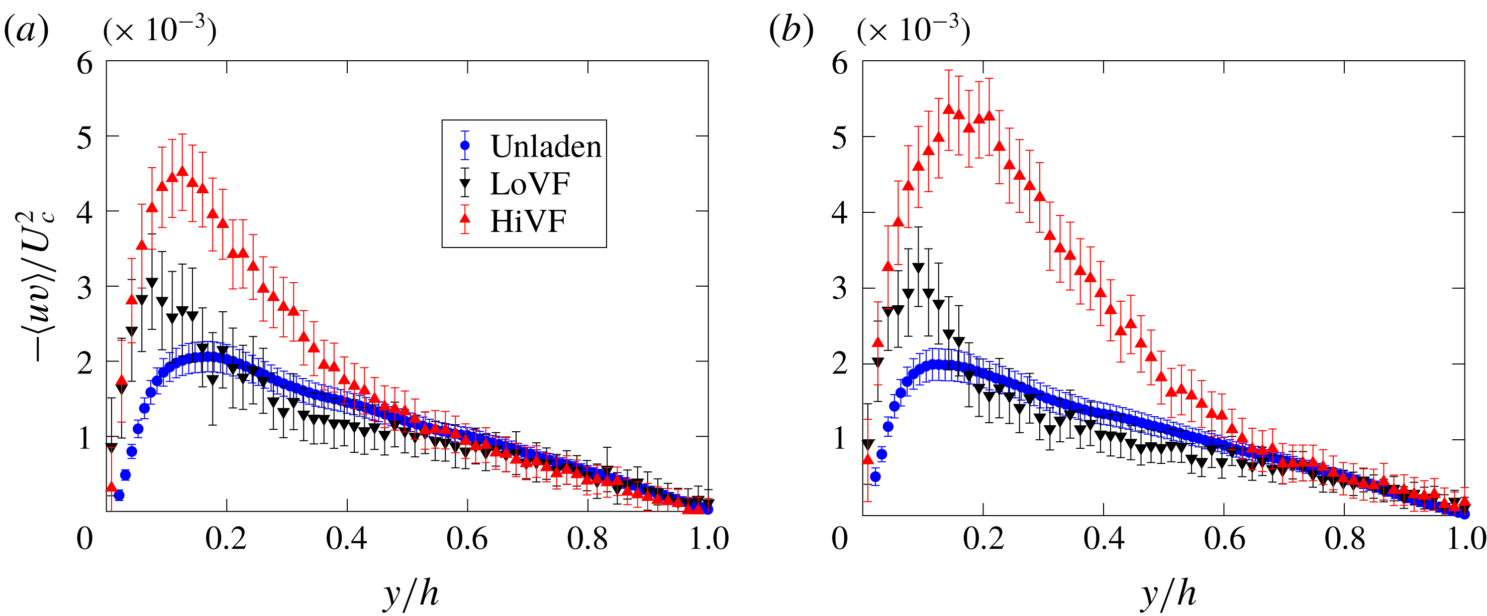
In figure 11 we present profiles of the cross-correlation between the particle streamwise and wall-normal fluctuations, referred to as particle Reynolds shear stress, along with the unladen fluid counterpart. For LoVF, these are found to follow the trend of the unladen fluid in the channel core up to about
 $y/h=0.2$
, but visibly exceed those values in the near-wall region. A similar behaviour was reported in the vertical pipe flow of Caraman et al. (Reference Caraman, Borée and Simonin2003), whereas in horizontal flow studies such as Li et al. (Reference Li, Wang, Liu, Chen and Zheng2012) particle Reynolds stresses were above/below the fluid levels in the core/near-wall region. These discrepancies stress once more the consequential differences between configurations, in particular as pertains to the gravity force direction. The HiVF cases show again an earlier departure from the unladen fluid statistics and a more dramatic increase in correlation magnitude.
Profiles of particle Reynolds shear stress for (a) LoSt and (b) HiSt cases. Unladen fluid profiles are plotted for comparison.

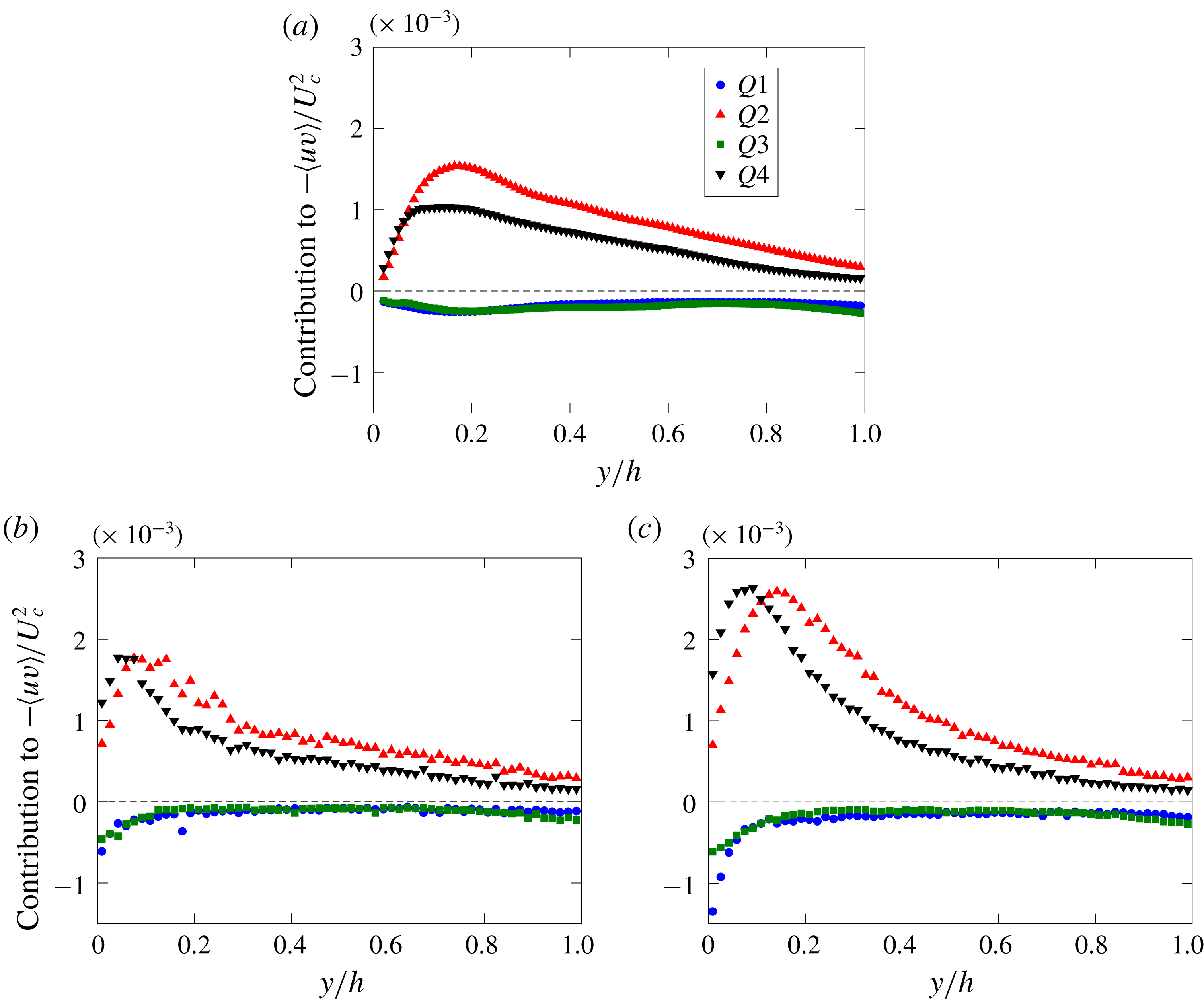
To explore this dynamic further, we perform a quadrant analysis in the (
 $u,v$
) plane. Following classic notation utilized in wall turbulence studies, we label events belonging to the four quadrants as Q1 (
 $u>,v>0$
), Q2 (
 $u<0,v>0$
), Q3 (
 $u<0,v<0$
) and Q4 (
 $u>,v<0$
). We report on the LoSt cases, which behave similarly to the HiSt cases. Figure 12(a) shows, for reference, the contributions to the Reynolds stresses for the unladen fluid velocity at the same Reynolds number. This highlights the predominance of the Q2 and Q4 events which contribute to positive turbulence production, with Q4 prevailing over Q2 for
 $y/h<0.06$
(or
 $y^{+}<15$
), and vice versa further from the wall (Kim, Moin & Moser Reference Kim, Moin and Moser1987). The particles (figure 12
b,c) follow a similar trend, but with noteworthy differences. The prevalence of Q4 events in the near-wall region is much more pronounced, which is consistent with sweeps being crucial in the process of trapping the particles near the wall (Marchioli & Soldati Reference Marchioli and Soldati2002). This is in stark contrast with the result of Li et al. (Reference Li, Wang, Liu, Chen and Zheng2012): they found overwhelmingly higher probability of Q2 events near the floor of their horizontal channel, where gravity caused much more frequent wall rebounds. For HiVF, both Q2 and Q4 contributions are similarly enhanced, but the cross-over point is farther from the wall compared to LoVF: the region where particles are swept towards the wall is wider, which corresponds to a more intense turbophoretic drift, a stronger near-wall peak of concentration and a depletion of the centreline peak (see figure 5). For this case also Q3 is remarkably large near the wall, probably a consequence of particles colliding with each other and with the wall (Righetti & Romano Reference Righetti and Romano2004).
Contribution of each quadrant of the (
 $u,v$
) plane to the Reynolds shear stresses for (a) unladen fluid, and inertial particles for (b) the LoSt-LoVF case and (c) the LoSt-HiVF case.

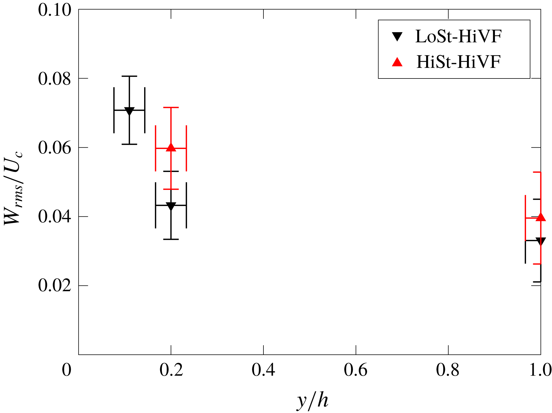
For completeness, we present in figure 13 the r.m.s. of the particle spanwise velocity fluctuations from the wall-parallel measurements. At
 $y/h=0.2$
and 1, the values are consistent with the fluid
 $W_{rms}$
in the DNS of Moser et al. (Reference Moser, Kim and Mansour1999) for
 $Re_{\unicode[STIX]{x1D70F}}=180$
and 395 at the same wall-normal locations, which are expected to be close to the unladen fluid values in the present case. The sharp increase at
 $y/h=0.11$
for the LoSt-HiVF case indicates again an augmented fluctuation of the particle velocity near the wall with higher loading, at odds with previous two-way coupled simulations (Li et al.
Reference Li, McLaughlin, Kontomaris and Portela2001; Nasr et al.
Reference Nasr, Ahmadi and McLaughlin2009).
Profile of r.m.s. spanwise particle velocity for LoSt-HiVF and HiSt-HiVF cases, obtained from the wall-parallel measurements expanded in § 3.2.

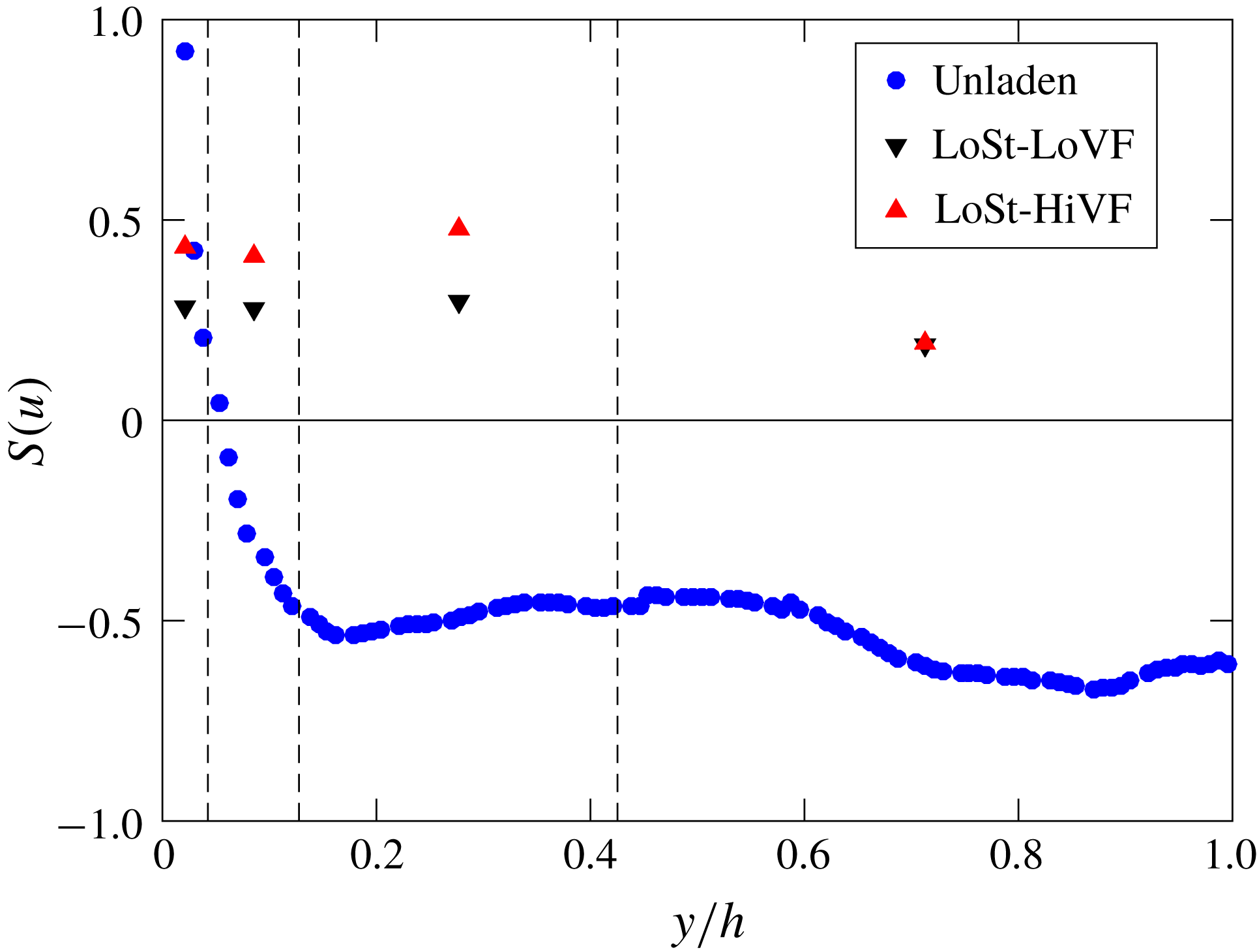
We conclude this section by considering the skewness of the streamwise velocity fluctuations for the inertial particles, in comparison with the unladen fluid. Figure 14 shows data for the LoSt cases (HiSt cases displaying the same trend). To improve convergence, the particle profiles are binned in four regions, each displaying fairly homogeneous behaviour and roughly corresponding to the inner layer (
 $y^{+}<10$
), buffer layer (
 $10<y^{+}<30$
), log layer (
 $30<y^{+}<100$
) and outer layer (
 $100<y^{+}<235$
). The unladen fluid streamwise fluctuations have positive skewness in the inner layer and part of the buffer layer, and negative elsewhere as expected (e.g. Kim et al.
Reference Kim, Moin and Moser1987). On the other hand, the inertial particles show positive skewness across the channel height, irrespective of volume fraction. Considering the flow is in the direction of gravity, this may be due to a tendency of the particles in the channel core to favour the downward side of turbulent eddies, as is known to happen in homogeneous turbulence (Wang & Maxey Reference Wang and Maxey1993). We will return to this point in § 3.2.2.
Profile of the skewness of the particle streamwise velocity fluctuations in the LoSt-LoVF and LoSt-HiVF cases. Unladen fluid profile is plotted for comparison. The vertical dashed lines demarcate the regions over which the particle–laden data are averaged.

3.2 Wall-parallel measurements
We leverage the wall-parallel plane imaging to investigate the instantaneous spatial organization of the particles and their velocity distribution. Streamwise/spanwise planes are especially suitable for this analysis, as they extend along homogeneous directions and thus allow for the efficient calculation of statistics that are unbiased by spatial gradients. We employ two-point quantities such as radial distribution functions (RDFs) and two-point Eulerian velocity correlations of streamwise velocity fluctuations, as well as tessellation techniques such as Voronoi diagrams and box-counting. We do not report here on the spanwise velocity fluctuation correlations in the wall-parallel planes, as the spanwise displacements are not sufficiently larger than the uncertainty to yield accurate second-order statistics. These tools are used to investigate the wall-parallel plane at the centreline (centreplane) and the near-wall plane at
 $y/h=0.11$
. The analysis is carried out only for the HiVF cases, for which the number of particles is sufficient to provide sufficient spatial resolution and statistical accuracy. While this does not allow direct assessment of the volume fraction effect on such quantities, it does bring useful insight to the particle spatial distribution in the regime for which the interphase coupling is expected to be more complex.
3.2.1 Two-point statistics
We use RDFs to describe the scale-by-scale concentration in the area surrounding a generic particle, compared to a uniform distribution (Sundaram & Collins Reference Sundaram and Collins1997). For two-dimensional distributions such as those obtained by planar imaging, this can be written as (e.g. Wood, Hwang & Eaton Reference Wood, Hwang and Eaton2005)
 $$\begin{eqnarray}g(r)=\frac{\langle N_{r}/A_{r}\rangle }{N/A},\end{eqnarray}$$
where
 $N_{r}$
represents the number of particles within an annulus of radius
 $r$
and area
 $A_{r}$
, and
 $N$
is the total number of particles within the planar domain of area
 $A$
. In the presence of clustering, the RDF is expected to increase above unity for decreasing
 $r$
, and the range over which it remains significantly greater than unity approximately indicates the length scale over which clustering occurs. We compute RDFs by binning particle pairs in equally spaced annuli of radial width 0.5 mm (
 $0.03h$
). An edge-correction strategy is needed for particles near the image boundaries. Omitting annuli that cross the image boundary limits the maximum separation to the radius of the domain-inscribed circle, reducing the number of usable particle pairs with increasing separations and thus affecting the large-scale characterization. We instead mirror the particle field across the image boundaries, so that the same number of annuli is used for each particle location. The maximum separation then equals the full image size, introducing only small biases near the boundaries (Salazar et al.
Reference Salazar, De Jong, Cao, Woodward, Meng and Collins2008; de Jong et al.
Reference de Jong, Salazar, Woodward, Collins and Meng2010; Petersen et al.
Reference Petersen, Baker and Coletti2019). To avoid projection biases at separations below the illuminated volume thickness (Holtzer & Collins Reference Holtzer and Collins2002), we only present
 $g(r)$
for
 $r>1.1~\text{mm}$
.
This ‘global’ (i.e. omnidirectional) definition of RDF does not discriminate between different directions of the separation
 $r$
. We also calculate ‘directional’ RDFs, in which the separations are oriented either streamwise or spanwise. This allows us to characterize the streamwise and spanwise extent of the highly concentrated particle structures. Additionally, we calculate the angular distribution function (ADF; see Gualtieri, Picano & Casciola Reference Gualtieri, Picano and Casciola2009; Nicolai, Jacob & Piva Reference Nicolai, Jacob and Piva2013) which is obtained by binning the planar domain in polar coordinates (
 $r,\unicode[STIX]{x1D703}$
):
 $$\begin{eqnarray}g(r,\unicode[STIX]{x1D703})=\left.\left\langle \frac{N_{r,\unicode[STIX]{x1D703}}(r,\unicode[STIX]{x1D703})}{A_{r,\unicode[STIX]{x1D703}}(r,\unicode[STIX]{x1D703})}\right\rangle \right/\left(\frac{N}{A}\right).\end{eqnarray}$$
Here
 $\unicode[STIX]{x1D703}=0^{\circ }$
and
 $\unicode[STIX]{x1D703}=90^{\circ }$
correspond to spanwise and streamwise directions, respectively. We use equally spaced annuli of radial width
 $0.03h$
and divide each of them in 24 azimuthal sectors of area
 $A$
(in which we count
 $N$
particles). Streamwise and spanwise homogeneities are leveraged to limit the analysis to one quarter of the
 $(r,\unicode[STIX]{x1D703})$
circle.
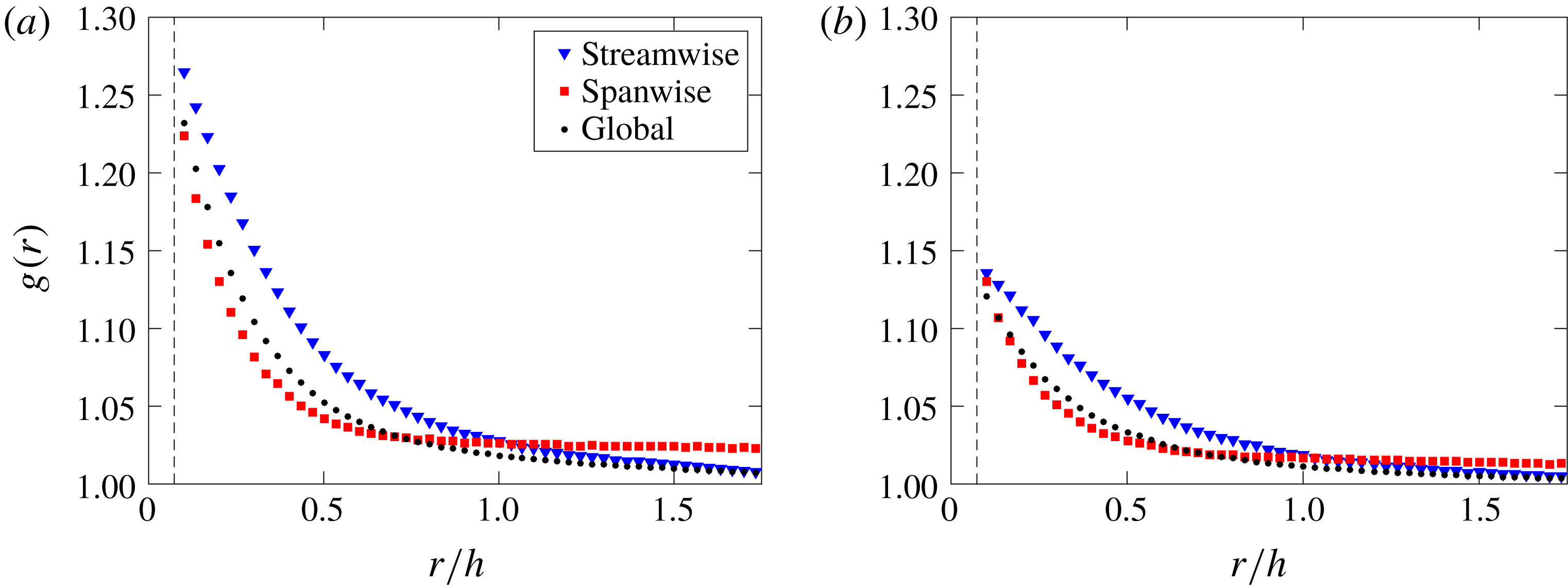
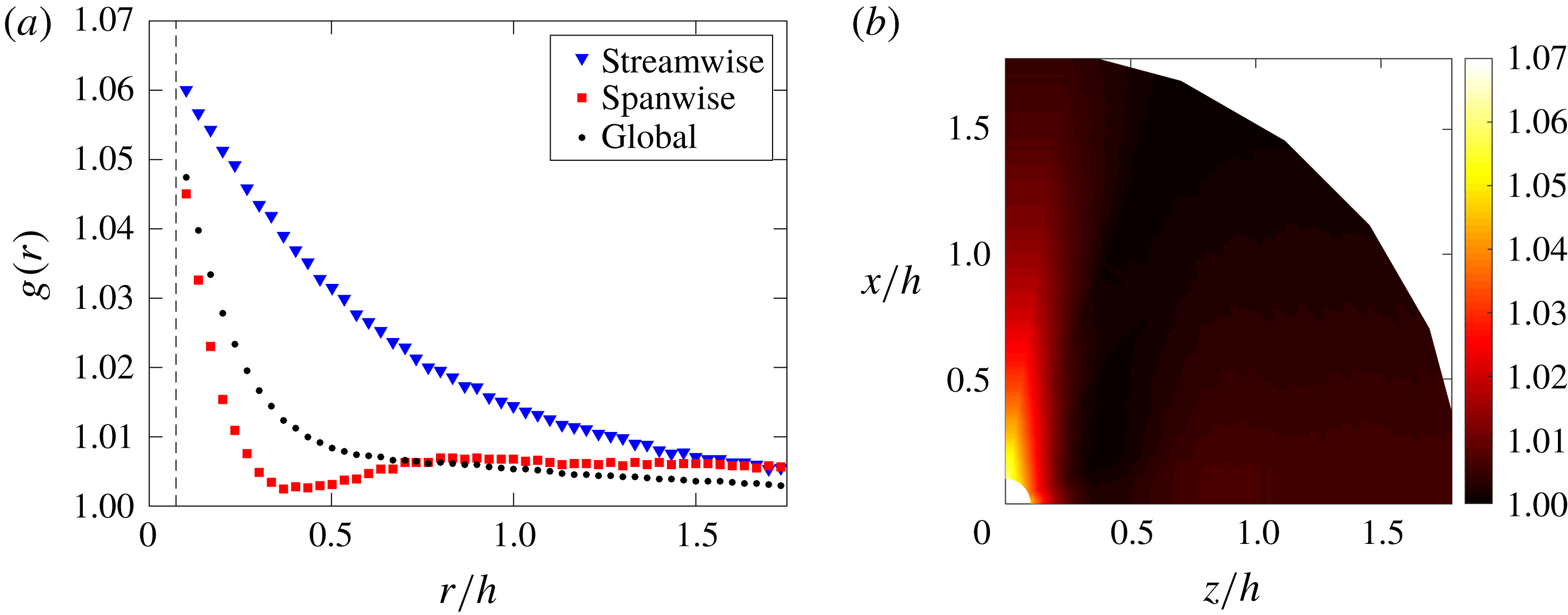
We first consider the wall-parallel plane at the centreplane. Figure 15 shows RDFs (global and directional) for LoSt and HiSt cases. The global RDFs indicate that clustering extends over similar length scales for both cases, but it is significantly more pronounced for LoSt. This is not unexpected since the latter is closer to the condition
 $St_{\unicode[STIX]{x1D702}}\sim 1$
, which was shown to produce more intense clustering in homogeneous turbulence (Wang & Maxey Reference Wang and Maxey1993; Wood et al.
Reference Wood, Hwang and Eaton2005) and at the centreplane of channel flows (Fessler et al.
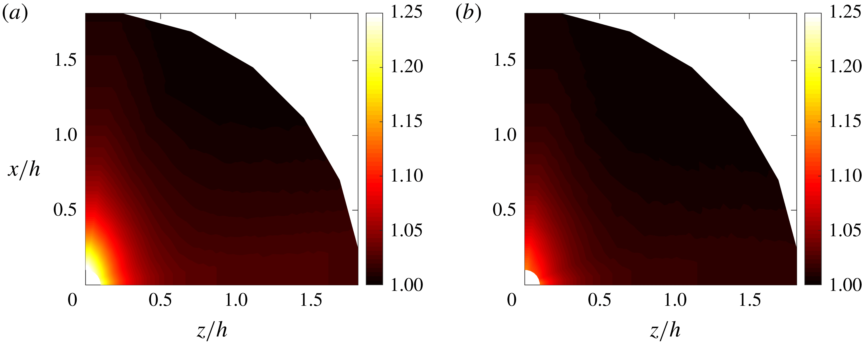
Reference Fessler, Kulick and Eaton1994). The directional RDFs also indicate that the clusters are more elongated in the streamwise than in the spanwise direction. The spanwise RDF remains somewhat above unity throughout the field, indicating that some structure in the particle distribution persists over large scales in that direction. This general picture is confirmed by the ADFs in figure 16, which also show how the particle field becomes more quickly decorrelated for separations in direction
 $\unicode[STIX]{x1D703}\sim 45^{\circ }$
.
Global and directional RDFs along the centreplane for (a) LoSt-HiVF and (b) HiSt-HiVF. The vertical dashed line indicates the laser sheet thickness.

Angular distribution functions along the centreplane for (a) LoSt-HiVF and (b) HiSt-HiVF.

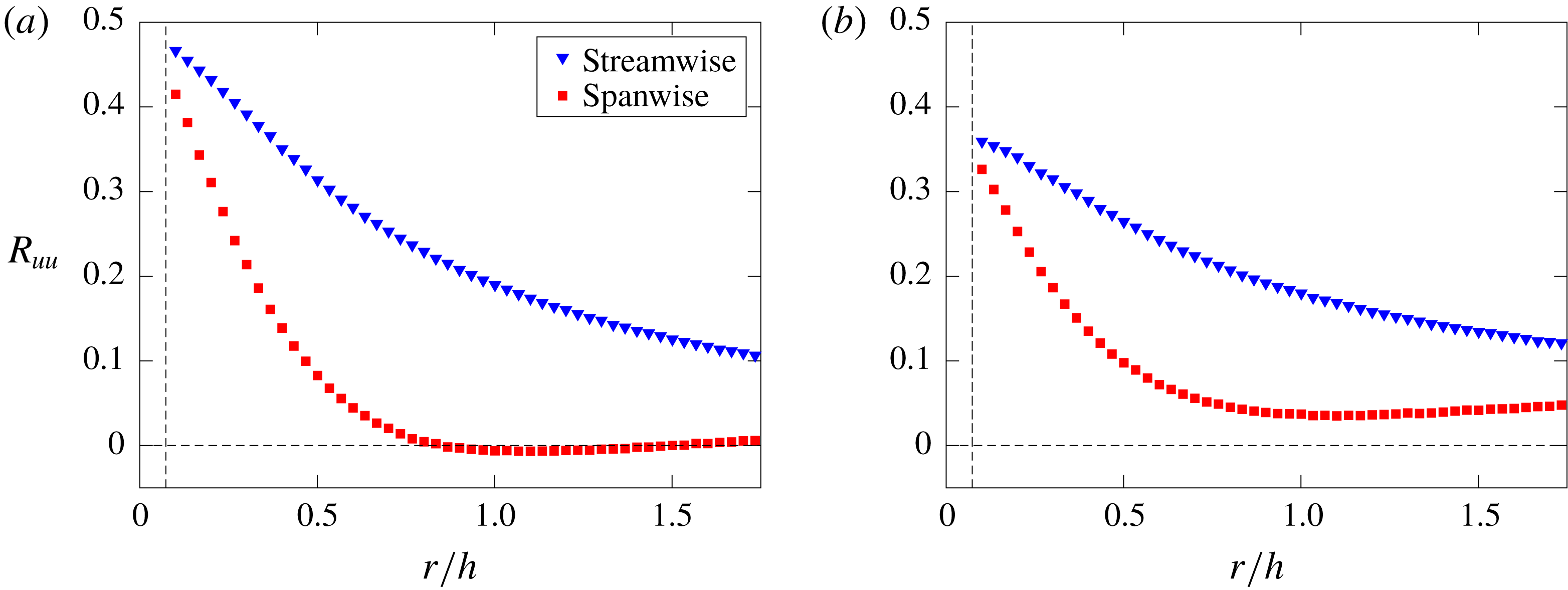
Two-point correlation of streamwise velocity fluctuations with separations in streamwise and spanwise directions along the centreplane, for (a) LoSt-HiVF and (b) HiSt-HiVF. The vertical dashed line indicates the laser sheet thickness.

We next consider the two-point Eulerian velocity correlations, which provide information on the level of spatial coherence of the particle motion. We follow Fevrier, Simonin & Squires (Reference Fevrier, Simonin and Squires2005), who in turn borrowed the formalism proposed by Sundaram & Collins (Reference Sundaram and Collins1999), and write the general expression for the correlation between the streamwise velocity fluctuations of particles
 $m$
and
 $n$
, normalized by their velocity variance:
 $$\begin{eqnarray}R_{uu}(r)=\frac{\langle u^{(m)}u^{(n)}\mid \boldsymbol{x}=\boldsymbol{x}_{\boldsymbol{p}}^{(\boldsymbol{m})};\boldsymbol{x}+\boldsymbol{r}=\boldsymbol{x}_{\boldsymbol{p}}^{(\boldsymbol{n})}\rangle }{\langle u^{2}\rangle }.\end{eqnarray}$$
Here
 $\boldsymbol{x}$
is the location within the measurement plane,
 $\boldsymbol{x}_{\boldsymbol{p}}^{(\boldsymbol{i})}$
is the position of the generic
 $\boldsymbol{i}$
th particle,
 $\boldsymbol{r}$
is the separation vector connecting the particle pair (
 $m,n$
) and angle brackets represent ensemble-averaging over all particle pairs. Boldface denotes vectorial quantities. The calculation is implemented with the same processing routine used for the RDFs and ADFs (which contains the information on the particle pair mutual positions). Again, we calculate both ‘directional’ correlations, in which the separation vector is either streamwise or spanwise, and polar correlations, which span the (
 $r,\unicode[STIX]{x1D703}$
) space.
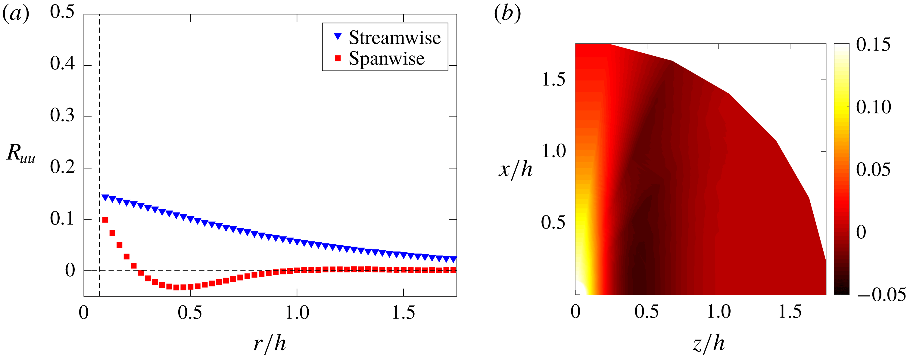
Figure 17 displays the directional velocity correlations evaluated at the centreplane. For both LoSt and HiSt cases, the normalized values do not approach unity for vanishingly small separations. (This is also confirmed by data points for separations smaller than the laser sheet thickness, not shown because inherently less accurate.) This indicates that a significant portion of the particle velocity is not spatially correlated. This is in line with the mesoscopic Eulerian formalism introduced by Fevrier et al. (Reference Fevrier, Simonin and Squires2005), according to which inertial particle motion consists of two components: a contribution from the underlying turbulent velocity field, spatially correlated; and a quasi-Brownian velocity distribution, random and as such spatially uncorrelated. The latter is rooted in the particle inertia, in particular the memory of interactions with distant eddies. This results in different velocities of arbitrarily close particles, possibly enhancing collision rates, and is consistent with the concepts of caustics and sling effect (Wilkinson & Mehlig Reference Wilkinson and Mehlig2005; Bewley, Saw & Bodenschatz Reference Bewley, Saw and Bodenschatz2013; Reeks Reference Reeks2014). The gap between unity and
 $R_{uu}$
for vanishing separations is a measure of the fraction of random uncorrelated motion (Fevrier et al.
Reference Fevrier, Simonin and Squires2005; Vance, Squires & Simonin Reference Vance, Squires and Simonin2006). This framework has been employed in numerous theoretical and numerical studies to analyse and model different particle–laden flows, from turbulent channels (Vance et al.
Reference Vance, Squires and Simonin2006) to homogeneous turbulence (Meneguz & Reeks Reference Meneguz and Reeks2011) and planar jets (Masi et al.
Reference Masi, Simonin, Riber, Sierra and Gicquel2014). However, experimental observations of Eulerian particle velocity correlations have been rarely reported, Khalitov & Longmire (Reference Khalitov and Longmire2003) and Sahu et al. (Reference Sahu, Hardalupas and Taylor2014) being notable exceptions. Figure 17 indicates that HiSt particles display a larger uncorrelated component of the motion than LoSt, consistent with the mesoscopic Eulerian formalism.
From figure 17 one also observes that more inertial particles show a slower decay of velocity correlation with increasing separation, according to the picture of high-
 $St$
particles responding to larger turbulent scales. Moreover, the streamwise fluctuations are significantly more correlated in streamwise than spanwise directions. This is consistent with the idea that the correlated particle motion is dictated by the turbulent flow. Indeed, if one defines integral scales of the fluctuating particle velocity based on the separation at which the correlation drops by 50 %, the transverse scale appears to be roughly half the longitudinal one, similar to the expected behaviour of the underlying turbulence. The polar diagrams of
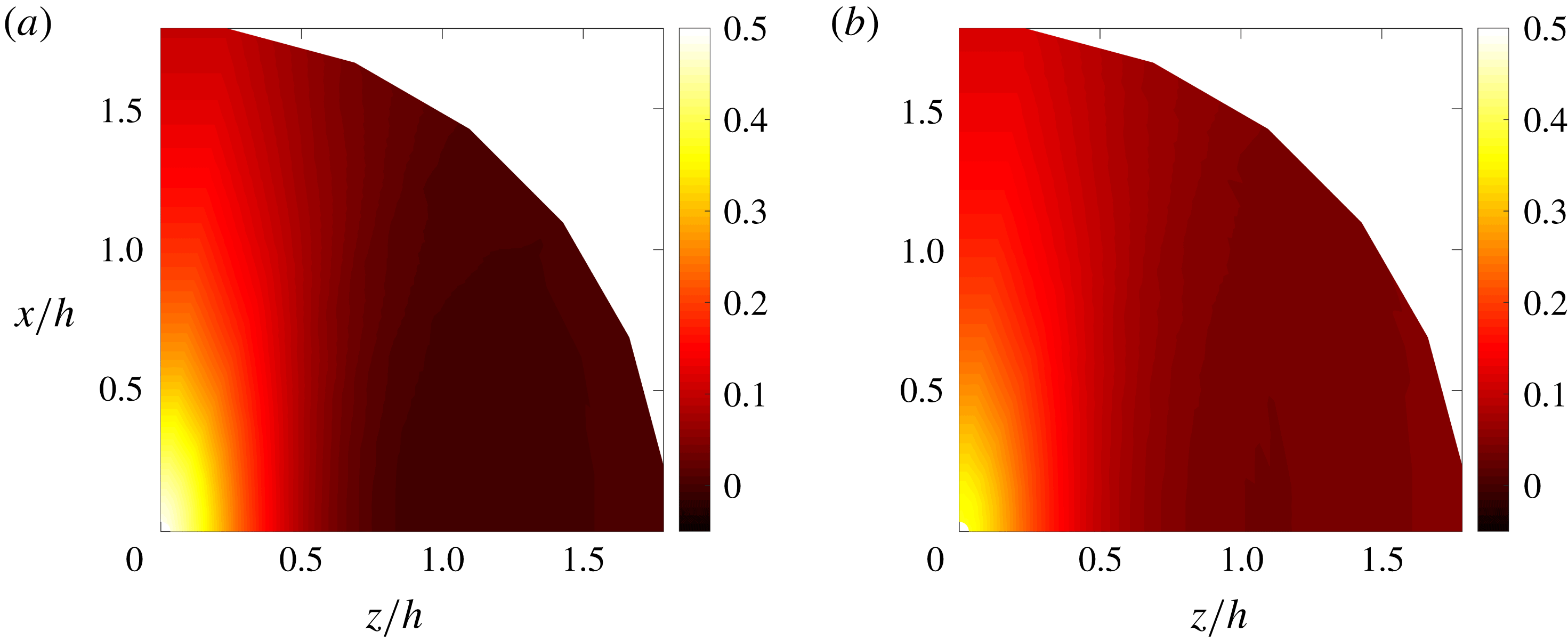
 $R_{uu}$
in figure 18 confirm this picture, and further suggest that the particle motion is organized in large streamwise-elongated structures, whose half-width is about
 $0.5h$
. This is consistent with the spatial particle distributions as deduced from the RDFs.
Polar map of streamwise velocity two-point correlation along the centreplane, for (a) LoSt-HiVF and (b) HiSt-HiVF.

(a) Global and directional RDFs and (b) ADF for the LoSt-HiVF case along the near-wall plane.

(a) Two-point correlation of streamwise velocity fluctuations with separations in the near-wall plane. (b) Spatial velocity correlation map for streamwise velocity fluctuations of inertial particles in the near-wall plane.

After considering two-point statistics at the centreplane, we move our attention to the near-wall plane. We focus on the LoSt case, for which more significant preferential concentration is expected. Figure 19 displays global and directional RDFs and ADFs, which indicate how the particles are arranged in elongated streaks, multiple channel heights in length. Indeed, due to the highly anisotropic spatial distribution of the particles in this region, the global RDFs provide limited insight compared to the directional representations. The amplitude of the peak is significantly smaller than at the centreplane, indicating generally weaker clustering. This is consistent with the fact that particles have much larger response times than the near-wall turbulent scales. As mentioned in the Introduction, several authors used point-particle simulations to investigate the near-wall structure of the particle distributions in regimes for which turbophoresis and preferential concentration are intense (McLaughlin Reference McLaughlin1989; Zhang & Ahmadi Reference Zhang and Ahmadi2000; Rouson & Eaton Reference Rouson and Eaton2001; Marchioli & Soldati Reference Marchioli and Soldati2002; Soldati & Marchioli Reference Soldati and Marchioli2009; Sardina et al.
Reference Sardina, Schlatter, Brandt, Picano and Casciola2012a
; Bernardini Reference Bernardini2014). They found thin streaks separated by
 $\mathit{O}(100)$
wall units, which roughly correspond to fluid-phase low-speed streaks in wall-bounded flows (Robinson Reference Robinson1991), and are even longer than the fluid streaks. Experimental observations of particle streaks have been sporadic, and mostly limited to snapshot realizations (Kaftori et al.
Reference Kaftori, Hetsroni and Banerjee1995a
; Niño & Garcia Reference Niño and Garcia1996). The present measurements provide quantitative information on such structures: the spanwise RDF shows a minimum at separations of
 ${\sim}0.3h$
or 70 wall units (which can be interpreted as a measure of the streak width) and recovery to a local maximum at
 ${\sim}0.75h$
or 175 wall units (a measure of the streak spacing). These values are somewhat larger than those found in numerical studies at similar regimes. Moreover, the RDF amplitude we observe at small separations is much smaller than in computations, as will be confirmed by instantaneous particle distributions shown later. Besides the above-mentioned limitations of the point-particle modelling approach, the differences can be partly attributed to the location and thickness of the observation region. Most numerical studies report on streaks along thin slices within the viscous sublayer, which are challenging to isolate in laboratory experiments. Here the imaged particles are contained in a slab of thickness
 ${\sim}1.1~\text{mm}$
centred at
 $y/h\sim 0.11$
, thus in the approximate range
 $y^{+}=17{-}34$
. The projection through this thickness may significantly influence the apparent concentration in a region of large wall-normal gradients. Future quantitative comparisons with simulations should take into account such finite thickness of the illumination volume.
When compared to the centreplane, the two-point velocity correlations at
 $y/h=0.11$
show an even stronger uncorrelated component of the motion as shown in figure 20. The uncorrelated velocity component near the wall is expected to increase with increasing particle inertia (Fevrier et al.
Reference Fevrier, Simonin and Squires2005), and indeed in the near-wall region the particle response time is much larger than the local time scale of the turbulence (i.e.
 $St^{+}\gg 1$
). Besides inertia, interparticle and wall–particle collisions may also contribute to the random particle motion (Vance et al.
Reference Vance, Squires and Simonin2006). In the HiVF regime considered, both near-wall concentration and deposition velocity are relatively high (§ 3.1), thus collisions may play a significant role in the observed partitioning between correlated and uncorrelated velocity. The negative lobe of velocity correlation along the spanwise direction indicates that the particles are arranged in a streaky fashion, alternating positive and negative streamwise velocity fluctuations. The longitudinal extent of those features cannot be precisely assessed from the present measurements, but the long tail of the correlation function in the streamwise direction suggests they can extend beyond the field of view. The trends in figure 20 are quantitatively similar to the RDFs and ADF in figure 19, implying that the fluctuations of particle velocity and concentration are simultaneous. We will elaborate on this point in the next subsection.
3.2.2 Domain tessellation
In order to further investigate the instantaneous distribution of the inertial particle positions and velocities, we apply domain tessellation methods along the wall-parallel planes. These have been widely used to study clustering of inertial particles in turbulence (Monchaux et al.
Reference Monchaux, Bourgoin and Cartellier2012). These approaches should be considered complementary to RDFs, since the latter are strictly two-point quantities, while tessellations are sensitive to the multi-particle arrangement. The simplest method is perhaps box-counting, which consists of dividing the domain into boxes of equal size, counting the particles in each box, and comparing the probability distribution function (p.d.f.) of the number of particles per box against the Poisson distribution expected for randomly distributed particles. This technique provides a simple scalar measure of the amount of clustering and has been fruitfully exploited in experimental studies (Fessler et al.
Reference Fessler, Kulick and Eaton1994; Aliseda et al.
Reference Aliseda, Cartellier, Hainaux and Lasheras2002). In recent years, the Voronoi tessellation method (Monchaux, Bourgoin & Cartellier Reference Monchaux, Bourgoin and Cartellier2010) has gained broader favour: the domain (in our case the two-dimensional image) is divided into cells associated with individual particles, each cell containing the set of points closer to that particle than to any other. The inverse of the area of each cell equals the local instantaneous concentration,
 $C=1/A_{cell}$
. The method has been used in several experimental and numerical studies of wall-bounded particle–laden flows (Garcia-Villalba et al.
Reference Garcia-Villalba, Kidanemariam and Uhlmann2012; Nilsen et al.
Reference Nilsen, Andersson and Zhao2013; Nicolai et al.
Reference Nicolai, Jacob and Piva2013; Rabencov et al.
Reference Rabencov, Arca and van Hout2014). Compared to the box-counting method, it has the advantage of not requiring an extrinsic/arbitrary length scale (the box size).
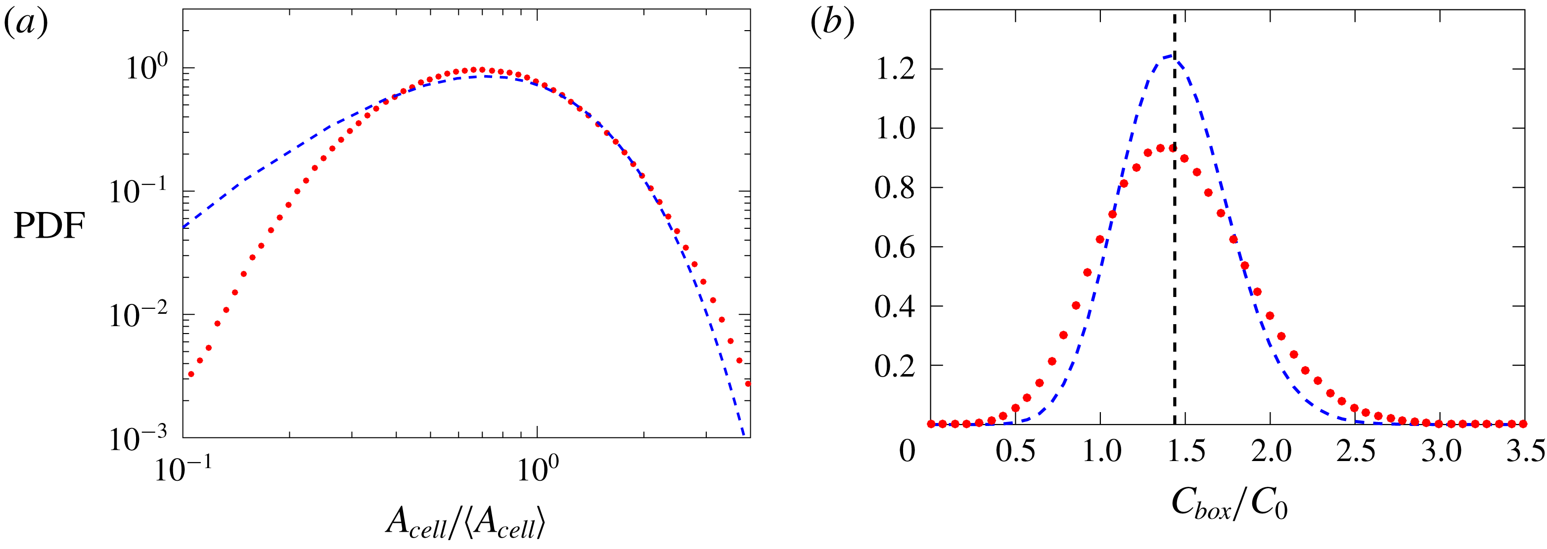
Here we adopt the Voronoi tessellation to investigate the particle distribution along the centreplane. Figure 21(a) shows a sample instantaneous realization for the LoSt-HiVF case, with Voronoi cells drawn around each particle. In figure 21(c) the p.d.f. of the cell areas (normalized by its ensemble average) is plotted. As typical of inertial particles clustered by turbulence, the distribution is much wider compared to a random Poisson process, which is well approximated by a
 $\unicode[STIX]{x1D6E4}$
distribution (Ferenc & Néda Reference Ferenc and Néda2007). The p.d.f. of the Voronoi cells is found to closely follow a log-normal distribution (Monchaux et al.
Reference Monchaux, Bourgoin and Cartellier2010; Petersen et al.
Reference Petersen, Baker and Coletti2019), which allows us to characterize the curve by its standard deviation
 $\unicode[STIX]{x1D70E}_{A}$
. The latter is a metric of the amount of clustering: LoSt and HiSt cases are found to have
 $\unicode[STIX]{x1D70E}_{A}/\langle A_{cell}\rangle =0.78$
and 0.70, respectively, confirming that the former has stronger tendency to produce clusters.
(a) Voronoi tessellation diagram in a sample centreplane realization, with (b) highlighted clusters (coherent clusters in cyan). (c) Probability distribution function of the Voronoi cell areas
 $A_{cell}$
along the centreplane (red circles), compared with a
 $\unicode[STIX]{x1D6E4}$
distribution (blue dashed line); the vertical dashed line indicates the threshold
 $A_{cell}^{\ast }$
.

The topology and behaviour of clusters of highly concentrated particles are relevant to the interphase coupling, especially in view of significant collective back-reaction of the dispersed phase on the carrier fluid. We therefore analyse individual clusters (coloured in figure 21
b), defined as connected groups of particles whose Voronoi cell areas are smaller than a threshold value
 $A_{cell}^{\ast }$
(figure 21
c): the latter is taken as the value below which the probability of finding small cell areas is higher than for randomly distributed particles (Monchaux et al.
Reference Monchaux, Bourgoin and Cartellier2010). To avoid spurious edge effects, we apply the additional constraint that the area of the cells neighbouring a cluster also be smaller than
 $A_{cell}^{\ast }$
(Zamansky et al.
Reference Zamansky, Coletti, Massot and Mani2016). The sum of the areas of all cells belonging to each cluster is taken as its ‘cluster area’,
 $A_{C}$
.
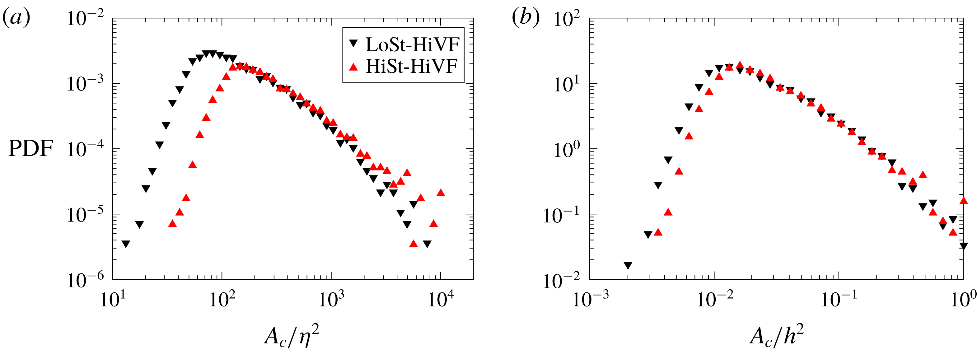
The p.d.f.s of the cluster areas for the LoSt-HiVF and HiSt-HiVF cases in the channel centreplane, normalized by (a) the Kolmogorov scale corresponding to the flow velocity and (b) the square of the channel half-height,
 $h^{2}$
.

Figure 22 shows the probability distribution of cluster areas
 $P(A_{C})$
along the centreplane for LoSt and HiSt, the p.d.f. in figure 22(a) normalized by the corresponding Kolmogorov length scale and in figure 22(b) normalized by the square of the channel half-height,
 $h^{2}$
. Consistent with previous experimental studies, typical sizes are
 $\mathit{O}(10\unicode[STIX]{x1D702})$
(Aliseda et al.
Reference Aliseda, Cartellier, Hainaux and Lasheras2002), although such estimates may be affected by the number of particles in the system (Petersen et al.
Reference Petersen, Baker and Coletti2019). HiSt particles tend to cluster over larger sets, consistent with their limitation of only responding to the larger scales of turbulence. Above a certain size the probability distributions approach a power-law decay, which is a feature of fractality or geometric self-similarity, indicating a fractal-like formation process due to turbulence (Baker et al.
Reference Baker, Frankel, Mani and Coletti2017). This was clearer in the homogeneous turbulence studies of Sumbekova et al. (Reference Sumbekova, Cartellier, Aliseda and Bourgoin2017) and Petersen et al. (Reference Petersen, Baker and Coletti2019), probably due to a combination of limited number of particles in the field of view and limited dynamic spatial range at the present Reynolds numbers. Figure 22(b) shows that normalizing by the channel half-height produces a remarkable collapse of the LoSt and HiSt cases. This may suggest that, while particle clustering at the present
 $St$
is influenced by small-scale turbulence, the energetic scales of fluid motion also play a major role (as recently argued, for example, by Petersen et al. (Reference Petersen, Baker and Coletti2019)). Moreover, this may indicate that the cluster size is significantly influenced by the channel geometry. Indeed, an a priori estimate of the controlling effect of channel walls on clustering is often deduced from the ratio of the channel height to a characteristic cluster size,
 $L_{c}=\unicode[STIX]{x1D70F}_{p}^{2}g$
(Capecelatro et al.
Reference Capecelatro, Pepiot and Desjardins2014). Here
 $L_{c}=2.8~\text{mm}$
and
 $2h/L_{c}=10.6$
, and the value of
 $L_{c}$
is close to the peak of p.d.f. (
 $A_{c}$
). We remark, however, that the definition of
 $L_{c}$
is usually adopted in much denser regimes than the present one, being independent of the air-flow characteristics. Further studies with different particle properties and turbulence conditions should discriminate whether
 $L_{c}$
is an appropriate scale for highly dilute systems.
Following Baker et al. (Reference Baker, Frankel, Mani and Coletti2017), we define ‘coherent clusters’ as those objects large enough to display a scale-invariant topology, i.e. in the range of
 $P(A_{C})$
that approximates the power-law decay. Smaller objects are considered as randomly occurring groups of particles, not necessarily brought together by the underlying turbulent flow. We conventionally set the cutoff at the respective maxima of
 $P(A_{C})$
for both LoSt and HiSt, noting that the choice of twice larger cutoffs does not qualitatively change the observed trends. Besides the physical interpretation discussed in Baker et al. (Reference Baker, Frankel, Mani and Coletti2017), this step allows us to discard clusters formed by only a few particles (too small for a meaningful topological description).
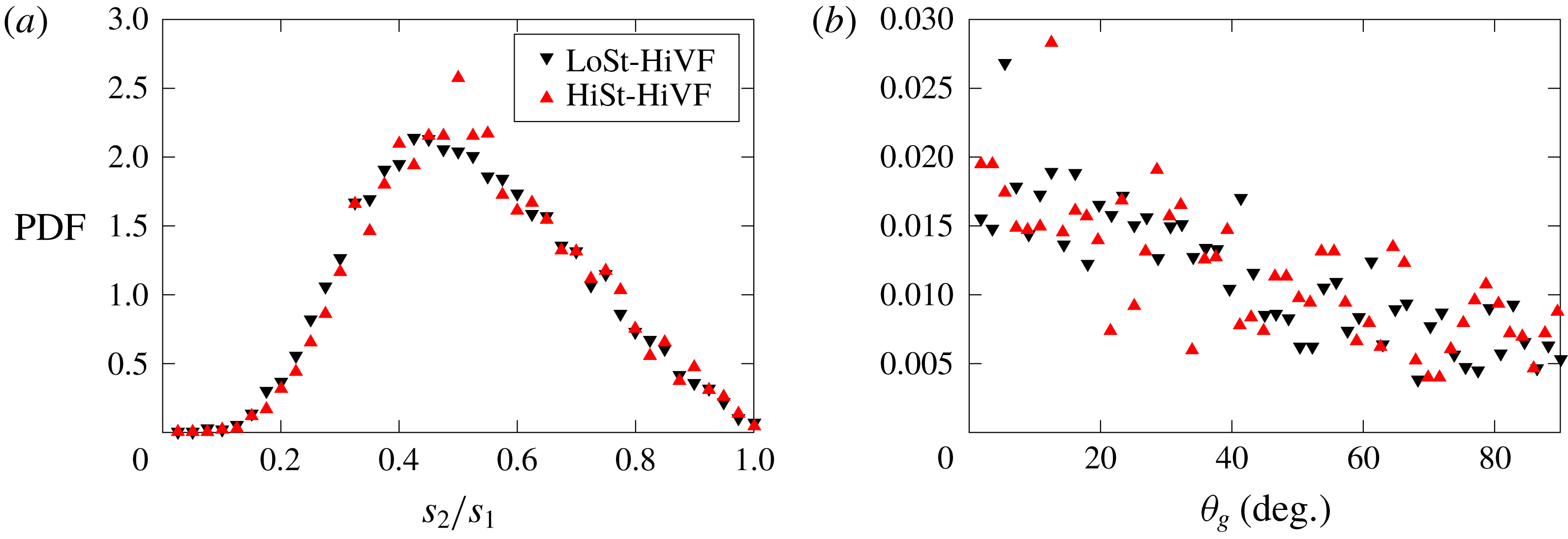
The p.d.f.s of (a) the SVD-based aspect ratio and (b) the angle between the primary axis and the vertical for the LoSt-HiVF and HiSt-HiVF cases.

We use the singular value decomposition (SVD) method introduced by Baker et al. (Reference Baker, Frankel, Mani and Coletti2017) to probe the shape and spatial orientation of the coherent clusters. The SVD provides the principal axes and corresponding singular values for a particle set: the primary axis lies along the direction of greatest particle spread from the cluster centroid, the secondary axis being orthogonal to it. The corresponding singular values
 $s_{1}$
and
 $s_{2}$
measure the spread along the respective axes. In figure 23(a) the p.d.f. of the aspect ratio
 $s_{2}/s_{1}$
is plotted for LoSt (differences with HiSt are marginal). The limit values 0 and 1 correspond to particles arranged in a straight line and in a perfect circle, respectively. The distribution is quantitatively similar to that reported by Petersen et al. (Reference Petersen, Baker and Coletti2019) for clusters settling in homogeneous turbulence. The peak ratio between 0.4 and 0.55 reflects a tendency to form somewhat elongated objects. Figure 23(b) illustrates the probability distribution of the primary axis orientation, measured by the angle of the latter with the vertical (
 $\unicode[STIX]{x1D703}_{g}$
). The peak at
 $\unicode[STIX]{x1D703}_{g}=0$
indicates a tendency of the (coherent) clusters to be aligned with gravity (and thus the direction of motion). This behaviour was also reported in homogeneous turbulence studies (Baker et al.
Reference Baker, Frankel, Mani and Coletti2017; Petersen et al.
Reference Petersen, Baker and Coletti2019) and is consistent with the directional RDFs and ADFs presented above.
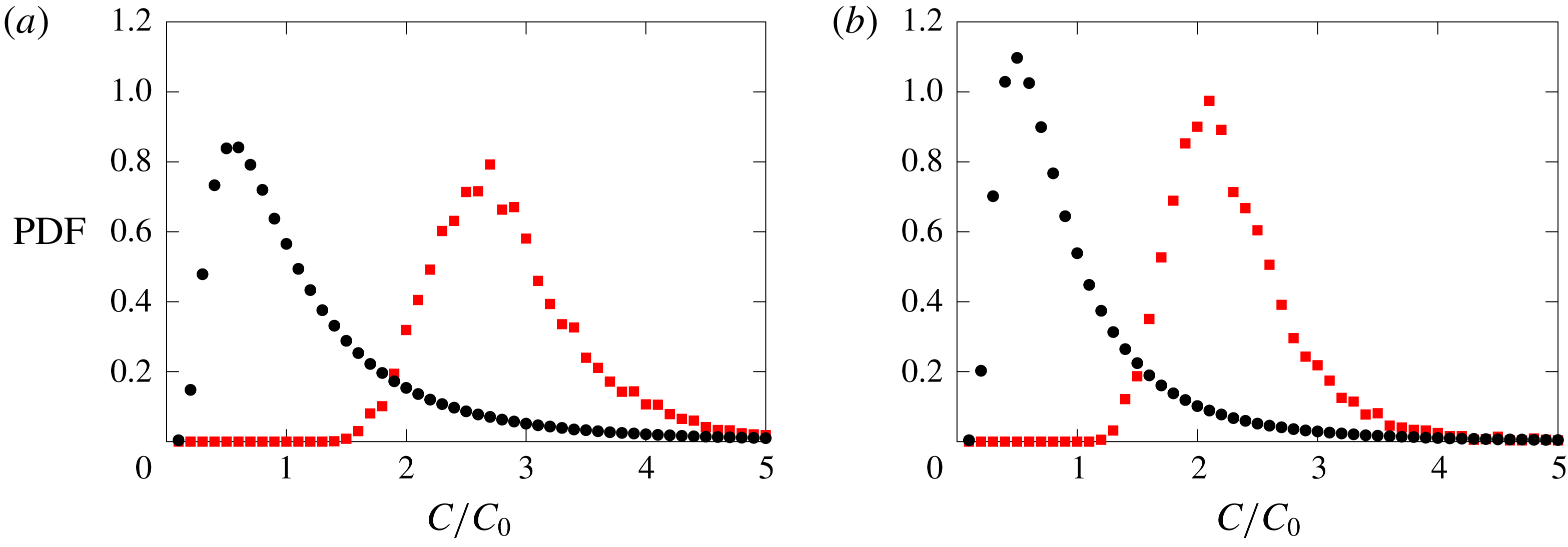
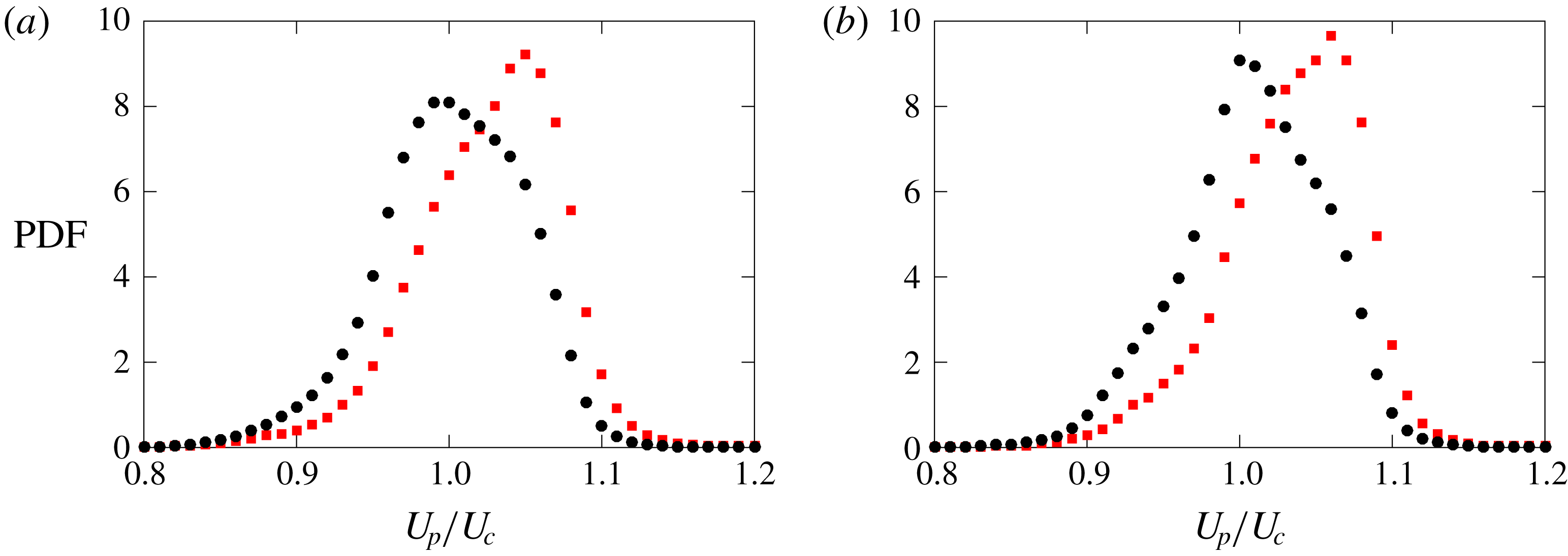
The p.d.f.s of normalized in-cluster (red squares) and global (black circles) concentrations for (a) LoSt-HiVF and (b) HiSt-HiVF.

The local particle concentration within clusters can be significantly higher compared to the global value
 $C_{0}$
(Baker et al.
Reference Baker, Frankel, Mani and Coletti2017). Figure 24 shows p.d.f.s of
 $C/C_{0}$
associated with the particles within coherent clusters, compared to the unconditional distribution: the peaks in the p.d.f. for the clustered particles are about four times higher for HiSt and almost five times higher for LoSt. Besides reaffirming that the latter case displays more intense clustering, these plots indicate how the in-cluster concentration can be substantial, such that two-way-coupling (and possibly four-way-coupling) effects may be at play.
(a) The same instantaneous realization as in figure 21, with the Voronoi cell colour-coded by the local particle streamwise velocity. (b) Joint p.d.f. of streamwise velocity and concentration at the centreplane for the LoSt-HiVF case. The dashed lines indicate the velocity and concentration values averaged along the centreplane. The black contour line indicates the p.d.f. level at 0.005.

The p.d.f.s of normalized in-cluster (red squares) and global (black circles) velocities for (a) LoSt-HiVF and (b) HiSt-HiVF in the channel centreplane.

The travelling velocity of the clustered particles is also important to the transport process. Figure 25(a) depicts the same instantaneous realization as in figure 21, with the Voronoi cells now colour-coded by the streamwise velocity of the respective particles. The more concentrated regions appear associated with higher velocities, as confirmed by the joint p.d.f. for LoSt-HiVF (figure 25 b): the local particle concentration and streamwise velocity are positively correlated. For a more quantitative account, shown in figure 26 are the p.d.f.s of the streamwise velocity for particles belonging to coherent clusters along the centreplane, as well as for all particles in the field of view. The clustered particles travel downward measurably faster than the generic particles. The explanations may be two-fold: on the one hand, particles may be favouring the downwash side of turbulent eddies, according to the picture of preferential sweeping originally proposed by Maxey (Reference Maxey1987) and later demonstrated by the simulations of Wang & Maxey (Reference Wang and Maxey1993) and recently by the experiments of Petersen et al. (Reference Petersen, Baker and Coletti2019); on the other hand, the highly concentrated clusters may be exerting a collective drag force on the fluid, in turn enhancing their vertical velocity as shown in the numerical simulations of Bosse, Kleiser & Meiburg (Reference Bosse, Kleiser and Meiburg2006) and Frankel et al. (Reference Frankel, Pouransari, Coletti and Mani2016).
In principle, the Voronoi method may also be used to identify the highly concentrated structures near the wall. However, figure 27(a) shows how the p.d.f. of the Voronoi cell areas measured along the near-wall plane is in fact narrower than for randomly distributed particles. This may be an artifact due to the relatively high concentration near the wall: particles very close to each other might be identified as one, reducing the probability of detecting small cell areas. Alternatively, the actual topology of the particle field, expected to be organized in streaks, could result in a ‘crystallized’ pattern with a relatively regular arrangement of cells (and thus a narrow p.d.f. of their area). Either way, the Voronoi tessellation method (in its standard form) does not appear as a suitable tool to study clustering in the present near-wall particle fields. We therefore resort to the box-counting approach: we tessellate the domain with square boxes of size 60 wall units or
 ${\sim}0.18h$
, and in figure 27(b) we plot the p.d.f. of the concentration in each box
 $C_{box}$
, comparing it with the Poisson distribution expected for randomly located particles. The relatively broad distribution indicates that the particles are indeed clustered over scales of the order of the box size. The choice of the latter is informed by the width of the particle streaks as estimated from the RDF analysis in the previous subsection, although it is verified that varying it by a factor of two yields similar conclusions. The box index
 $BI=(\unicode[STIX]{x1D70E}-\unicode[STIX]{x1D70E}_{Poisson})/\unicode[STIX]{x1D707}$
(where
 $\unicode[STIX]{x1D707}$
and
 $\unicode[STIX]{x1D70E}$
indicate mean and standard deviation of the distribution, respectively, and
 $\unicode[STIX]{x1D70E}_{Poisson}$
is the standard deviation of the Poisson distribution) is a comparative measure of clustering. Near the wall we find
 $BI=0.05$
, while
 $BI=0.2$
at the centreplane. The latter (consistent with the results of Fessler et al. (Reference Fessler, Kulick and Eaton1994)) confirms the indication from the RDF analysis that clustering in the channel core is significantly more intense.
(a) The p.d.f. of the Voronoi cell areas
 $A_{cell}$
along the near-wall plane (red circles), compared with a
 $\unicode[STIX]{x1D6E4}$
distribution (blue dashed line). (b) The p.d.f. of particle concentration in square boxes of size
 $0.18h$
used to tessellate the near-wall plane (red circles) compared to a Poisson distribution (blue dashed line).

Figure 28(a) shows an instantaneous realization of the near-wall particle field, colour-coded with the mean particle velocity in each square box of the tessellation. The visual impression of elongated slow-velocity streaks is in line with the RDF results. In figure 28(b) we plot a joint p.d.f. of local particle concentration and streamwise velocity, based on values averaged in each box. The apparent negative correlation contrasts with the centreplane trend in figure 25(b), indicating a tendency of the highly concentrated particles to travel slower than the average. Combined with the RDFs, ADFs and two-point correlations reported above, this confirms the picture of particles accumulating in slow-moving streaks.
(a) Sample realization at the near-wall plane, tessellated by
 $0.18h\times 0.18h$
boxes and colour-coded by the mean local streamwise particle velocity within the boxes. (b) Joint p.d.f. of streamwise velocity and box-based concentration at the near-wall plane for the LoSt-HiVF case. The dashed lines indicate the velocity and concentration averaged along the near-wall plane. The black contour line indicates the p.d.f. level at 0.005.

4 Conclusions
We have reported on a series of experiments conducted on a vertical turbulent channel flow at
 $Re_{\unicode[STIX]{x1D70F}}=235$
and 335, in which particle–laden air flows downward. Several aspects of the configuration are chosen to provide a canonical case: smooth walls, streamwise development, relatively large aspect ratio of the cross-section and small size-selected particles with
 $St_{\unicode[STIX]{x1D702}}=\mathit{O}(10)$
and
 $St^{+}=\mathit{O}(100)$
. Care is taken to keep the experimental parameters under strict control, including the smoothness of the walls and the particle mass loading. The latter is varied across what is usually considered the boundary between one-way and two-way coupling. Using laser imaging we have investigated in detail the particle spatial distribution and velocity, gaining new insight expected to be useful to reach a predictive understanding of particle–laden wall-bounded flows. Here we summarize and discuss the main findings.
At volume fractions
 $\mathit{O}(10^{-6})$
, the particles show a distinct, although relatively mild, tendency to segregate near the wall, with the concentration displaying a second maximum at the channel centreline. The results are consistent with turbophoresis acting down the gradients of turbulence intensity, and in particular of
 $V_{rms}$
as proposed by Young & Leeming (Reference Young and Leeming1997). At volume fractions
 $\mathit{O}(10^{-5})$
, the near-wall peak is much more pronounced and the centreline maximum is absent, indicating more vigorous turbophoretic drift towards the wall. The increase of near-wall segregation with mass loading is opposite to that reported in previous two-way-coupled point-particle simulations.
The mean velocity profiles show particles travelling faster than the unladen fluid in the immediate vicinity of the wall, resulting in an effective slip velocity. Away from the wall, the more dilute case has particles following a profile similar to the unladen air velocity. In the denser case, the particles are measurably slower up to
 $y/h\sim 0.4$
(0.6) for the lower (higher) Stokes number. Both streamwise and wall-normal velocity fluctuations of the particles exceed those of the unladen fluid near the wall; in the denser case the effect is much more significant and extended to larger wall distances. The wall-normal fluctuations do not vanish close to the wall, and lead to estimates of the deposition velocity in line with the expectations in the dilute case, but several times larger in the dense case. The particle Reynolds shear stress follows a similar behaviour to the normal stresses: it equals the unladen fluid stress in the channel core, but exceeds it when approaching the wall to a degree that depends on the loading. A quadrant analysis reveals that the prevalence of Q4 events (the equivalent of ‘sweeps’ for the fluid motion) is enhanced in the near-wall region compared to the unladen fluid, suggesting that fluid sweeps are key in the particle segregation process. The effects above are similarly displayed by all cases investigated here, but are more evident for the higher
 $St$
.
For the denser cases, the spatial distributions of the particle positions and velocities are analysed over wall-parallel planes using both two-point statistics and tessellation techniques, providing further details of the particle organization and dynamics. In the channel core, the particles show a strong propensity to cluster, forming somewhat elongated objects preferentially aligned in the vertical streamwise direction. Clustering is more intense for the cases closer to the condition
 $St_{\unicode[STIX]{x1D702}}\sim 1$
, although at higher
 $St$
the clusters tend to be larger (Petersen et al.
Reference Petersen, Baker and Coletti2019). Groups of particles above a certain size range (‘coherent clusters’; Baker et al.
Reference Baker, Frankel, Mani and Coletti2017) reach concentrations several times higher than the global mean, and tend to travel/fall faster than the non-clustered particles. This suggests that, although the flow in the channel core is a poor approximation of homogeneous isotropic turbulence, the classic phenomena of preferential concentration (Squires & Eaton Reference Squires and Eaton1991) (or other more recent mechanisms that explain clustering; see Goto & Vassilicos (Reference Goto and Vassilicos2008) and Bragg & Collins (Reference Bragg and Collins2014)) and preferential sweeping (Wang & Maxey Reference Wang and Maxey1993) are at play. In the near-wall region the particles are observed to form elongated streaks, several channel heights in length and spaced by
 $\mathit{O}(100)$
wall units (although the limited range of Reynolds numbers does not allow us to determine a conclusive scaling). Those streaks tend to move slower than the generic particles, supporting the view that they are coupled to fluid low-speed streaks typical of wall turbulence. The particle velocity contains a significant component of random uncorrelated motion. In agreement with the mesoscopic Eulerian formalism introduced by Fevrier et al. (Reference Fevrier, Simonin and Squires2005), this Brownian-like motion is more prominent for higher
 $St$
and in the near-wall region, where the particle response time is much longer than the turbulent time scales. In general, we note that the differences between the particle behaviour near and far from the wall, already remarkable in the present regimes, are expected to be magnified at higher
 $Re_{\unicode[STIX]{x1D70F}}$
.
Taken together, these results are consistent with a scenario in which the increase in volume fraction from
 $\mathit{O}(10^{-6})$
to
 $\mathit{O}(10^{-5})$
triggers two-way and (locally) four-way coupling effects. In particular, the particle back-reaction may alter the turbulence structure in ways that enhance the turbophoretic drift towards the wall (e.g. by enhancing the peak of turbulence intensity and/or displacing it away from the wall). In turn, the higher near-wall concentration may promote interparticle and wall–particle collisions. These would damp the particle kinetic energy, causing them to travel more slowly but enhancing their velocity fluctuations, as observed. Moreover, the inelastic collisions may prevent the particles from escaping the near-wall region (Hrenya & Sinclair Reference Hrenya and Sinclair1997). In the absence of simultaneous fluid measurements, this and other possible scenarios remain speculative. Future studies should fill this gap, for example using phase separation techniques (Kiger & Pan Reference Kiger and Pan2000; Khalitov & Longmire Reference Khalitov and Longmire2002; Capone, Romano & Soldati Reference Capone, Romano and Soldati2015; Petersen et al.
Reference Petersen, Baker and Coletti2019) to accurately measure fluid statistics in the near-wall region. This, however, is expected to be a challenging task: small inertial particles accumulating near the wall pose a major problem to imaging surrounding tracers. This can be partly alleviated by augmenting the spatial resolution, which is becoming possible thanks to the steady increase of the sensor size of available cameras (Discetti & Coletti Reference Discetti and Coletti2018).
Despite the relevance for practical applications and the understanding of particle–laden turbulence, previous experiments focused on the present regime have been scarce. The lack is unfortunate, especially given the need to validate point-particle models and the exorbitant cost of particle-resolved simulations. Contrasting our observations with previous numerical studies suggests that, while point-particle simulations capture many key features of the particle transport (e.g. Soldati & Marchioli Reference Soldati and Marchioli2009), the underlying hypotheses may be missing or misestimating some important aspects, especially concerning the two-way and four-way coupling. This is exemplified by the increased near-wall concentration measured for increasing mass loading, which is opposite to the trend found in past simulations. The limitations of point-particle methods in capturing the two-way coupling are well known (Eaton Reference Eaton2009; Balachandar & Eaton Reference Balachandar and Eaton2010) and have been assessed in detail by recent studies on homogeneous turbulence (Mehrabadi et al. Reference Mehrabadi, Horwitz, Subramaniam and Mani2018; Petersen et al. Reference Petersen, Baker and Coletti2019). Wall-bounded turbulence may pose even harder problems due to the spatially varying resolution. However, as mentioned in the Introduction, recent approaches are showing promising improvements. For example, Capecelatro & Desjardins (Reference Capecelatro and Desjardins2015) used a volume-filtering method to simulate the configuration of Benson et al. (Reference Benson, Tanaka and Eaton2005) and found satisfactory agreement. That case contained heavier particles than the present one, with a Stokes number likely too high to produce strong near-wall segregation and clustering. It would be interesting to evaluate this and other modelling strategies against the present data, also considering that the dilute and dense cases we investigated should allow isolation of one-way and two-way coupling issues. Importantly, given the significant role played by the dense regions in the momentum coupling, future comparisons with simulations should ideally include information on the spatial correlation of the particle field and the clustering properties. The moderate Reynolds number in our study may allow for a comparison with future particle-resolved simulations, which are becoming feasible even for relatively small particles (Schneiders, Meinke & Schröder Reference Schneiders, Meinke and Schröder2017).
Finally, we remark how the effect of interparticle and wall–particle collisions could also contribute to experimental–numerical discrepancies. As mentioned in § 2.1, the restitution coefficient may vary significantly depending on the collision velocity (Joseph et al.
Reference Joseph, Zenit, Hunt and Rosenwinkel2001; Gondret et al.
Reference Gondret, Lance and Petit2002). Following Gondret et al. (Reference Gondret, Lance and Petit2002), we can define a wall-collision Stokes number as
 $St_{p}=(1/9)Re_{p}\unicode[STIX]{x1D70C}_{p}/\unicode[STIX]{x1D70C}_{f}$
(where we used the fact that
 $V_{t}=\unicode[STIX]{x1D70F}_{p}g$
is of the order of the particle
 $V_{rms}$
close to the wall, the latter giving a scale for the wall-normal collision velocity). One finds
 $St_{p}=\mathit{O}(100)$
, which is in the range for which
 $e$
is a strong function of
 $St_{p}$
(Gondret et al.
Reference Gondret, Lance and Petit2002). Given the possibly large variance of the collision velocity and the role of inelastic collisions to enhance near-wall accumulation (Hrenya & Sinclair Reference Hrenya and Sinclair1997), the common assumption of a constant restitution coefficient might be inadequate.
Acknowledgements
This project is funded partly by the US Army Research Office (Division of Fluid Dynamics, grant nos W911NF-17-1-0366 and W911NF-18-1-0354) and partly by the Environment and Natural Resources Trust Fund of Minnesota.
Appendix A. Electrostatic dissipative acrylic
Electrostatic dissipative acrylic (SciCron Technologies) is used to build the optical test section, and the channel is provided with static discharge wires grounded to structural supports. This prevents the particles from accumulating upon impaction and building up unwanted roughness, an effect that has impacted past experiments (Benson et al. Reference Benson, Tanaka and Eaton2005). The importance of such precautions is illustrated in figure 29, where cumulative wall-normal profiles of particle concentrations are plotted in the higher volume fraction case. The details of how those measurements are obtained are given in § 2.2. When using standard acrylic walls, the concentration profiles start with a strong near-wall peak but drift in time, with particles migrating away from the wall. This is likely a consequence of wall deposition which leads to significant roughness (as verified by inspecting the wall surface at the end of the experiments), in turn altering the collision dynamics and ultimately enhancing particle dispersion towards the channel core. Using electrostatic dissipative acrylic virtually eliminates particle deposition (as also verified by direct wall inspection) and warrants consistent concentration profiles during each run and between different runs.
Wall-normal profiles of mean concentration for recordings of different durations, using (a) standard acrylic and (b) electrostatic dissipative acrylic. Here
 $C_{0}=880~\text{particles}~\text{cm}^{-3}$
, corresponding to
 $\unicode[STIX]{x1D719}_{v}=5\times 10^{-5}$
for both cases. Refer to table 2 for definitions on
 $y,h$
.

Appendix B. Coefficient of restitution
The coefficient of restitution,
 $e$
, for particle–wall collisions is measured by dropping individual glass beads from a height of 350 mm above a horizontal plate made of the same acrylic used for the test section. The particles reach steady-state terminal velocity before bouncing on the plate. This is achieved independently from the method of release due to the short free-fall stopping distance (of order
 $\unicode[STIX]{x1D70F}_{p}^{2}g\sim 3~\text{mm}$
). Particles are imaged at 2300 frames per second with a high-speed CMOS camera (VEO 640) paired with a 200 mm lens at f
 $/$
4, and tracked using the same method used for the particle–laden flow measurements. The coefficient of restitution
 $e$
is defined as the ratio of the wall-normal particle velocity just after and just before the collision, and is calculated averaging over five trials as shown in figure 30.
Particle height and vertical velocity data used for determining the restitution coefficient for particle–wall collisions over five trials. Positive velocity indicates upward motion. Tracks for each trial are shown in markers of different shapes and colours.