1. Introduction
The main purpose of this paper is to give an expression for the joint law of the endpoint and supremum of an Ornstein–Uhlenbeck process. The problem of finding such a joint law has attracted research since the late nineteenth century (see [Reference Sommerfeld20]). For a Brownian motion, the result is well known (see e.g. [Reference Karatzas and Shreve13]). More recently, in [Reference Escobar and Hernandez9], Escobar and Hernandez gave a method that allows one to find this joint density / distribution function for the minimum and endpoints for an n-dimensional Brownian motion with drift. The explicit solution in the two-dimensional case ( $n=2$) is given in [Reference He, Keirstead and Rebholz11]. For
 $n>2$, the method in [Reference Escobar and Hernandez9] works only in some cases. Coutin, Pontier, and Ngom [Reference Coutin, Pontier and Ngom6,Reference Ngom17] studied the case of a Lévy process, the sum of a Brownian motion with drift and a compound Poisson process. Coutin and Pontier [Reference Coutin and Pontier5] were interested in the joint law of an n-dimensional diffusion process and the running supremum of the first component. They found a partial differential equation satisfied by the joint density (but an Ornstein–Uhlenbeck process does not verify their assumption of bounded drift). Doney and Kyprianou [Reference Doney and Kyprianou8] studied the law for overshoots and undershoots when the process is a general Lévy process.
Let  $(X_t)_{t\geqslant 0}$ be an Ornstein–Uhlenbeck process driven by a Brownian motion. Many results on the first passage time of an Ornstein–Uhlenbeck process have been obtained. For instance, in [Reference Alili, Patie and Pedersen1], [Reference Linetsky15], and [Reference Lipton and Kaushansky16], the density function of the first hitting time to a fixed level by an Ornstein–Uhlenbeck process is given. Since hitting times and suprema are related, the cumulative distribution function of the supremum is obtained.
In our paper we study the joint density / distribution function
 \begin{equation*} \mathbb{P}\bigg(X_t\in \textrm{d} x, \sup_{0\leqslant u\leqslant t}X_u\leqslant m\bigg) \end{equation*}
where  $m,x\in\mathbb{R}$,
 $x\leqslant m$,
 $t\in\mathbb{R}_+^{*}$. This last formula is known only in the case
 $m=0$; it is easily obtained from [Reference Borodin and Salminen2, (1.0.6), (1.1.8), Chapter 7]. The probability
 $\mathbb{P}(X_{\tau}\in \textrm{d} x, \sup_{0\leqslant u\leqslant \tau}X_u\leqslant m )$, where
 $\tau$ is an exponential random variable independent of
 $(X_t)_{t\geqslant 0}$, can be obtained with [Reference Borodin and Salminen2, (1.0.5), (1.1.6), Chapter 7]. This is the Laplace transform of the requested distribution. As it is difficult to invert this Laplace transform, we propose a spectral approach.
The joint density / distribution function admits a density p which is a solution of a Fokker–Planck equation. To solve this equation a spectral method is used, and causes parabolic cylinder functions to appear (directly linked with the Hermite functions). Even if the joint law is an infinite expansion of special functions, it is easy to evaluate it numerically and it is faster than a Monte Carlo method. We then check that our result is consistent with those in [Reference Borodin and Salminen2] and [Reference Alili, Patie and Pedersen1].
The paper is organized as follows. In the next section we present the expression of the joint density / distribution of the endpoint and supremum of an Ornstein–Uhlenbeck process. We provide some numerical simulations to compare our results with a Monte Carlo method. Section 3 is devoted to the proof of this main theorem. Finally, Section 4 is concerned with the law of the supremum and its joint density with the process. Auxiliary results about Hermite functions and parabolic cylinder functions are provided in the Appendix.
2. Results
2.1. Context and notations
Let  $(B_t)_{t \geqslant 0}$ be a standard Brownian motion defined on a probability space
 $(\Omega,\mathcal{F},\mathbb{P} )$. We consider an Ornstein–Uhlenbeck (OU) process
 $(X_t)_{t\geqslant 0}$ solution of the following SDE:
 \begin{equation*}\begin{cases}\textrm{d} X_t =-kX_t \,\textrm{d} t+\textrm{d} B_t & t \geqslant 0 , \\[2pt] X_0 \sim \mu,\end{cases}\end{equation*}
where  $k \in \mathbb{R}_+^{*}$ and
 $\mu$ is a probability measure. We assume that
 $X_0$ and
 $(B_t)_{t \geqslant 0}$ are independent.
Let  $\mathbb{P}_{x_0}$ be the law of the process
 $(X_t)_{t \geqslant0}$ when
 $\mu \sim \delta_{x_0}$.
2.2. Main theorem
Our aim is to compute the joint law of the process and its supremum. However, as it is not easy to compute the joint density, we are first interested in the joint density / distribution
 \begin{equation*}\mathbb{P}\bigg(X_t\in \textrm{d} x, \sup_{0\leqslant u\leqslant t}X_u\leqslant m \bigg){,}\quad \text{where }t\in\mathbb{R}_+^{*}, (m,x)\in\mathbb{R}^2, x\leqslant m.\end{equation*}
The following theorem gives an expression for the joint density / distribution.
Theorem 1. We assume that  $\mu$ is a probability measure on
 $]-\infty, m]$,
 $m\in \mathbb{R}$, and set
 $p_0$ such that
 $\mu(\textrm{d} x)=p_0(x)\,\textrm{d} x$.
(i) For all
 $m\in \mathbb{R}$ and $t\in\mathbb{R}_+$, the probability $\mathbb{P}(X_t\in \textrm{d} x, \sup_{0\leqslant u\leqslant t}X_u\leqslant m )$ admits a density p with support in $]-\infty,m]$:
\begin{equation*}\mathbb{P}\bigg(X_t\in \textrm{d} x, \sup_{0\leqslant u\leqslant t}X_u\leqslant m\bigg)=p(m,x,t)\,\textrm{d} x.\end{equation*}
(ii) The density p solves the following Fokker–Planck equation, for all
$m\in \mathbb{R}$:
(1)\begin{equation} \begin{cases} \partial_t p(m,x,t)=k \partial_x(xp(m,x,t))+\tfrac{1}{2} \partial^2_{x^2}p(m,x,t) & (x,t)\in ]-\infty, m]\times \mathbb{R}_+^{*},\\[2pt] p(m,m,t)=0 & t \in \mathbb{R}_+^{*},\\[2pt] p(m,x, 0)=p_0(x) & x\in ]-\infty, m]. \end{cases}\end{equation}(iii) For
$(m,x)\in \{(z,y)\in\mathbb{R}^2 \mid z\geqslant y\}$, $t \in\mathbb{R}_+^{*} $, the density p can be expressed as
(2)where\begin{align}p(m,x,t)&=-\sqrt{2k}\,\textrm{e}^{-{{{kx^2}/{2}}}} \notag \\*&\quad\, \times \sum_{n=1}^{\infty} \,\textrm{e}^{-k {\nu_{n,m}} t} \dfrac{D_{{\nu_{n,m}}} ({-}x\sqrt{2k})\int_{-\infty}^m \,\textrm{e}^{{{{kz^2}/{2}}}}p_0(z)D_{{\nu_{n,m}}} ({-}z\sqrt{2k}) \,\textrm{d} z }{{\nu_{n,m}} D_{{\nu_{n,m}} -1} ({-}m\sqrt{2k})\partial_\nu D_{{\nu_{n,m}}}({-}m\sqrt{2k})},\end{align}$D_\nu$ is the parabolic cylinder function and $(\nu_{j,m})_{j \geqslant 1}$ is the ordered sequence of positive zeros of $\nu \mapsto D_{\nu} ({-}m\sqrt{2k})$ (details are given in the Appendix).









The proof of the theorem is postponed to Section 3. We start by studying some particular cases and consequences.
Remark 1. For  $(m,x)\in \{(z,y)\in\mathbb{R}^2 \mid z\geqslant y\}$,
 $t \in\mathbb{R}_+^{*} $, when
 $\mu \sim \delta_{x_0}$ and
 $x_0 \leqslant m$, we have
 \begin{equation}p(m,x,t)=-\sqrt{2k}\,\textrm{e}^{{{{k(x_0^2-x^2)}/{2}}}} \sum_{n=1}^{\infty} \,\textrm{e}^{-k {\nu_{n,m}} t} \dfrac{D_{{\nu_{n,m}}} ({-}x_0\sqrt{2k}) D_{{\nu_{n,m}}}({-}x\sqrt{2k})}{{\nu_{n,m}} D_{{\nu_{n,m}} -1} ({-}m\sqrt{2k})\partial_\nu D_{{\nu_{n,m}}}({-}m\sqrt{2k})}.\end{equation}
Since  $({-}X_t)_{t\geqslant 0}$ is also an OU process, the result could be extended by replacing m, x, and
 $x_0$ with
 $-m$,
 $-x$, and
 $-x_0$ in (3) to obtain the density of
 \begin{equation*}\mathbb{P}\bigg(X_t\in \textrm{d} x, \inf_{0\leqslant u\leqslant t}X_u\geqslant m \bigg).\end{equation*}
The expression of the joint density / distribution can be easily extended to an OU process depending on three parameters.
Corollary 1. Suppose that the OU process  $(X_t)_{t\geqslant 0}$ is a solution of the following SDE:
 \begin{equation*}\begin{cases}\textrm{d} X_t = (\phi-kX_t) \,\textrm{d} t+\sqrt{\beta}\,\textrm{d} B_t & t \geqslant 0,\\[3pt] X_0 \sim \mu,\end{cases}\end{equation*}
where  $\beta,k\in\mathbb{R}_+^{*}$ and
 $\phi\in \mathbb{R}$.
For  $(m,x)\in \{(z,y)\in\mathbb{R}^2 \mid z\geqslant y\}$,
 $t \in\mathbb{R}_+^{*} $, the density p can be expressed as
 \begin{align*}p(m,x,t)& =-\sqrt{\dfrac{2k}{\beta}} \,\textrm{e}^{-{{{k (x- {{{\phi}/{k}}})^2}/{(2\beta)}}}}\\*&\quad \times \sum_{n=1}^{\infty} \Bigg(\int_{-\infty}^{m- {{{\phi}/{k}}}} \,\textrm{e}^{{{{kz^2}/{(2\beta)}}}}p_0(z)D_{\nu_{n,m- {{{\phi}/{k}}}}}\Bigg({-}z\sqrt{\dfrac{2k}{\beta}}\Bigg) \,\textrm{d} z \Bigg)\,\textrm{e}^{-k \nu_{n,m- {{{\phi}/{k}}}} t} \\*&\quad \times \dfrac{D_{\nu_{n,m- {{{\phi}/{k}}}}}({-} (x- {{{\phi}/{k}}})\sqrt{2{{{k}/{\beta}}}})}{\nu_{n,m- {{{\phi}/{k}}}} D_{\nu_{n,m- {{{\phi}/{k}}}} -1} ({-}(m- {{{\phi}/{k}}})\sqrt{{{{2k}/{\beta}}}})\partial_\nu D_{\nu_{n,m- {{{\phi}/{k}}}}} ({-} (m- {{{\phi}/{k}}})\sqrt{{{{2k}/{\beta}}}})},\end{align*}
where  $D_\nu$ is the parabolic cylinder function and
 $(\nu_{j,m- {{{\phi}/{k}}}})_{j \geqslant 1}$ is the ordered sequence of positive zeros of
 \begin{equation*}\nu \mapsto D_{\nu}\bigg({-}\bigg(m- \dfrac{\phi}{k}\bigg)\sqrt{\dfrac{2k}{\beta}}\bigg).\end{equation*}
Proof. For  $t\in\mathbb{R}_+$, set
 $U_t\,:\!=X_{{{{t}/{\beta}}}}-{{{\phi}/{k}}}$ and
 $W_t\,:\!=\sqrt{\beta}B_{{{{t}/{\beta}}}}$ (which is thus a standard Brownian motion). Then the dynamic of
 $(U_t)_{t \geqslant 0}$ is
 \begin{equation*}\begin{cases}\textrm{d} U_t = -\dfrac{k}{\beta} U_t \,\textrm{d} t + \textrm{d} W_t & t \geqslant 0,\\[3pt]U_0 =X_0-\dfrac{\phi}{k} \in \mathbb{R}.\end{cases}\end{equation*}
We conclude with Theorem 1.  \hfill$\Box$
2.3. Numerical results
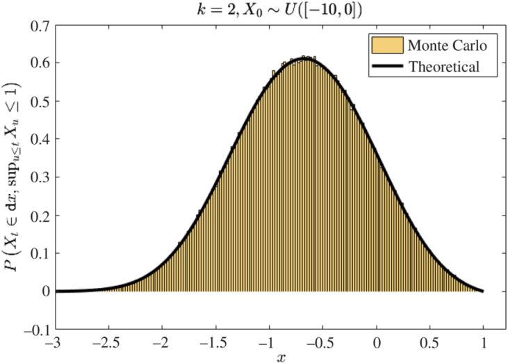
Even though formula (2) is an infinite sum of special functions, it is easy to evaluate it numerically.
The function  $x \mapsto p(m,x,t)$ is evaluated with expression (2) (or (3)) and is compared with a Monte Carlo method using
 $5 \times 10^5$ simulations and
 $\Delta_t = 10^{-4}$. Figures 1 and 2 plot
 \begin{equation*}\mathbb{P} \bigg(X_t\in \textrm{d} x, \sup_{0\leqslant u\leqslant t}X_u\leqslant m \bigg)\end{equation*}
for different parameters and initial laws with  $t=1$.
Comparison of expression (2) and a Monte Carlo method when  $m=1$,
 $X_0\sim \mathcal{U}([-10,0])$ and
 $k=2$.

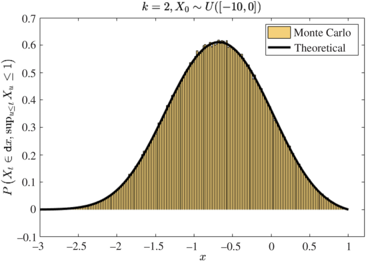
Comparison of expression (3) and a Monte Carlo method when  $m=-1$,
 $X_0=-2$ and
 $k=1$.

Last but not least, our formula is faster than a Monte Carlo method. Indeed, with a simple core, obtaining the whole function  $x \mapsto p(m,x,t)$ lasts around 23 seconds, whereas a Monte Carlo method with
 $10^5$ simulations lasts around 18 seconds,
 $2. 10^5$ simulations 34 seconds, and
 $10^6$ simulations 176 seconds.
2.4. Case $m=0$

If  $m=0$, the expression of the joint density / distribution can be simplified. Indeed, the zeros
 $(\nu_{n,0})_{n\geqslant0}$ of
 $\nu \mapsto D_\nu(0)$ are the positive odd integers (see the Appendix for more details). In this particular case, formula (3) can be simplified.
Proposition 1. We assume  $\mu \sim \delta_{x_0}$ and
 $x_0 \in \mathbb{R}_-$. For all
 $x\in \mathbb{R}_-$ and
 $t\in\mathbb{R}_+^{*}$, we have
 \begin{align*} & \mathbb{P}_{x_0}\bigg( X_t\in \textrm{d} x, \sup_{0\leqslant s\leqslant t}X_s\leqslant 0 \bigg)\\[3pt] &\quad =\sqrt{\dfrac{k}{\pi(1-\textrm{e}^{-2k t})}}\bigg[{\exp\biggl({-k\frac{(x-x_0\,\textrm{e}^{-k t})^2}{1-\textrm{e}^{-2k t}}}\bigg)-\exp\biggl({-k\frac{(x+x_0\,\textrm{e}^{-k t})^2}{1-\textrm{e}^{-2k t}}}\bigg)}\bigg]\,\textrm{d} x. \end{align*}
Proof. Without loss of generality, we take  $k=1$ in the proof. We use the results given in the Appendix. Let
 $x\in \mathbb{R}_-$ and
 $t\in\mathbb{R}_+^{*}$.
With (A11) and Proposition A.1., we have
 \begin{equation*}p(0,x,t)=\dfrac{2\textrm{e}^{{{{x_0^2-x^2}/{2}}}}}{\sqrt{\pi}}\sum_{n=0}^{\infty} \,\textrm{e}^{-(2n+1) t}\dfrac{D_{2n+1}({-}x_0\sqrt{2}) D_{2n+1}({-}x\sqrt{2})}{(2n+1)! }.\end{equation*}
We use (A10) and Fubini’s theorem (everything is clearly integrable):
 \begin{align*}p(0,x,t)& =-\dfrac{2\textrm{e}^{x_0^2}}{\pi\sqrt{\pi}}\sum_{n=0}^{\infty} \dfrac{2^{2n+1}\,\textrm{e}^{- (2n+1) t}}{(2n+1)!} \\[3pt] &\quad\, \times \int_0^\infty \int_0^\infty (uv)^{2n+1} \,\textrm{e}^{-(u^2+v^2)} \big(\textrm{e}^{2\textrm{i} v x_0 }-\textrm{e}^{-2\textrm{i} vx_0 }\big) \big(\textrm{e}^{2\textrm{i} u x }-\textrm{e}^{-2\textrm{i} ux }\big) \,\textrm{d} u \,\textrm{d} v .\end{align*}
We can invert integral and sum:
 \begin{align*}p(0,x,t)&=-\dfrac{2\textrm{e}^{x_0^2}}{\pi\sqrt{\pi}}\int_0^\infty \int_0^\infty \,\textrm{e}^{-(u^2+v^2)} \big(\textrm{e}^{2\textrm{i} v x_0 }-\textrm{e}^{-2\textrm{i} vx_0 }\big) \big(\textrm{e}^{2\textrm{i} ux }-\textrm{e}^{-2\textrm{i} ux }\big)\textrm{sh}(2uv\,\textrm{e}^{-t}) \,\textrm{d} u \,\textrm{d} v \\[3pt] &=-\dfrac{\textrm{e}^{x_0^2}}{\pi\sqrt{\pi}}\bigg[\int_{-\infty}^\infty \,\textrm{e}^{-v^2+2\textrm{i} vx_0}\int_{-\infty}^\infty \,\textrm{e}^{-u^2+2\textrm{i} ux+2uv\,\textrm{e}^{-t}}\,\textrm{d} u \,\textrm{d} v \\[3pt] &\quad\, - \int_{-\infty}^\infty \,\textrm{e}^{-v^2+2\textrm{i} vx_0 }\int_{-\infty}^\infty \,\textrm{e}^{-u^2+2\textrm{i} ux-2uv\,\textrm{e}^{-t}}\,\textrm{d} u \,\textrm{d} v \bigg].\end{align*}
Finally, [Reference Lebedev and Silverman14, formula (4.11.6)] gives
 \begin{align*}p(0,x,t)&=-\dfrac{\textrm{e}^{x_0^2}}{\pi} \bigg[\int_{-\infty}^\infty \,\textrm{e}^{-v^2+2\textrm{i} vx_0}\,\textrm{e}^{(\textrm{i} x+v\,\textrm{e}^{-t})^2} \,\textrm{d} v - \int_{-\infty}^\infty \,\textrm{e}^{-v^2+2\textrm{i} vx_0}\,\textrm{e}^{(\textrm{i} x-v\,\textrm{e}^{-t})^2}\,\textrm{d} v \bigg]\\[3pt] &=- \dfrac{\textrm{e}^{x_0^2-x^2}}{\sqrt{\pi(1-\textrm{e}^{-2t})}} \bigg[ {\exp\biggl( {-\frac{(x_0 + x\,\textrm{e}^{-t})^2}{1-\textrm{e}^{-2t}}}\bigg) - \exp\biggl( {-\frac{(x_0 - x\,\textrm{e}^{-t})^2}{1-\textrm{e}^{-2t}}}\bigg)}\bigg]\\[3pt] &= \dfrac{1}{\sqrt{\pi(1-\textrm{e}^{-2 t})}}\bigg[{\exp\biggl({-\frac{(x-x_0\,\textrm{e}^{- t})^2}{1-\textrm{e}^{-2 t}}}\bigg) -\exp\biggl({-\frac{(x+x_0\,\textrm{e}^{-t})^2}{1-\textrm{e}^{-2 t}}}\bigg)}\bigg].\tag*{$\Box$}\end{align*}
Remark 2. This is [Reference Borodin and Salminen2, formula (1.1.8), Chapter 7]. Note that there is a typographical error in the book.
3. Proof of the main theorem
This section is devoted to the proof of Theorem 1. The proof is divided into two parts. First we prove the existence of the density and the fact that it is a solution of the Fokker–Planck equation. The proof of the theorem relies on the second part, namely the resolution of this Fokker–Planck equation. Without loss of generality, we take  $k=1$.
Existence of the density and the Fokker–Planck equation
(i) The existence of the density is given by [Reference Delarue, Inglis, Rubenthaler and Tanré7, Lemma 2.1].
(ii) This is simply [Reference Jeanblanc, Yor and Chesney12, Proposition 5.4.3.1] with
$h\colon t \mapsto m$.

Resolution of the Fokker–Planck equation
(iii) Now we want to solve the Fokker–Planck equation. We use a spectral method inspired by [Reference Boyce and DiPrima3], [Reference Gardiner10], and [Reference Risken and Haken18]. For that purpose, we introduce two operators. Let
$m\in\mathbb{R}$.

Let  $\mathcal{D}(\textbf{{L}}_\textrm{FP})$ denote the space
 \begin{equation*}\bigg\lbrace f \in H^1(]-\infty,m]) \mid \bigg[x \mapsto\dfrac{\partial }{\partial x} (x f(x))+\dfrac12 f''(x)\bigg] \in L^2(]-\infty,m]), f(m)=0\bigg\rbrace.\end{equation*}
The Fokker–Planck operator  $\textbf{{L}}_\textrm{FP}$ is defined by
 \begin{equation*} \raisebox{14pt}{\hbox{${\textbf{{L}}_\textrm{FP}}\colon\ \ $}}\left|\ \begin{array}{c@{\ \ \ }c@{\ \ \ }c} {\mathcal{D}(\textbf{{L}}_\textrm{FP})}&\longrightarrow &{L^2(]-\infty,m])}\\[7pt] { f}&\longmapsto &{\bigg[\textbf{{L}}_\textrm{FP} f \colon x \mapsto\dfrac{\partial }{\partial x}(x f(x))+\dfrac12 f''(x)\bigg].}\end{array}\right. \end{equation*}
Let  $x \leqslant m$ and
 $t \in\mathbb{R}_+^{*}$. The goal is to find a basis
 $(\tilde{\varphi}_n)_{n \geqslant 1}$ of eigenvectors of
 $\textbf{{L}}_\textrm{FP}$ in order to write
 \begin{equation*}p(m,x,t)=\sum_{n=1}^{\infty }c_n(t) \tilde{\varphi}_n(x).\end{equation*}
The Fokker–Planck operator  $\textbf{{L}}_\textrm{FP}$ is not Hermitian. Then, to build this basis, we introduce the following operator
 $\textbf{{O}}$, related to
 $\textbf{{L}}_\textrm{FP}$ and defined by
 \begin{equation*} \raisebox{14pt}{\hbox{${\textbf{{O}}}\colon\ \ $}}\left|\ \begin{array}{c@{\ \ \ }c@{\ \ \ }c} {\mathcal{D}(\textbf{{L}}_\textrm{FP})}&\longrightarrow &{{L^2(]-\infty,m])}}\\[7pt] {f}&\longmapsto &{\bigg[\textbf{{O}}f \colon x \mapsto-\dfrac12x^2f(x) + \dfrac12 f''(x)\bigg].}\end{array}\right.\end{equation*}
As  $\textbf{{O}}$ is Hermitian, we can use classical results on the decomposition of Hermitian operators.
Moreover, we have a correspondence principle for the spectrum. The function  $\phi$ is an eigenfunction of
 $\textbf{{O}}$ with eigenvalue
 $\mu$ if and only if
 $x\mapsto \textrm{e}^{-{{{x^2}/{2}}}}\phi$ is an eigenfunction of
 $\textbf{{L}}_\textrm{FP}$ with eigenvalue
 $\mu+\frac12$.
Hilbert space basis of
 ${L^2 (]-\infty,m])}$. We prove that any function of
 ${L^2(]-\infty,m])}$ can be decomposed with respect to a Hilbert space basis of eigenvectors of
 $\textbf{{O}}$. Since it is not easy to prove this directly with the operator
 $\textbf{{O}}$, it is classical (see e.g. the proof of [Reference Brézis4, Theorem VIII.20]) to introduce the operator
 $\textbf{{T}}$ defined as
 \begin{equation*} \raisebox{10pt}{\hbox{${\textbf{{T}}}\colon\ \ $}}\left|\ \begin{array}{c@{\ \ \ }c@{\ \ \ }c} {{L^2(]-\infty,m])}}&\longrightarrow &{{L^2(]-\infty,m])}}\\[3pt] {g}&\longmapsto &{f_g,}\end{array}\right.\end{equation*}
where  $f_g$ is a solution of
 \begin{equation}
\begin{cases}
\tfrac12 f_g''(x)- \tfrac12 x^2f_g(x) =g(x) & x \in ]-\infty,m],\\[3pt]
f_g(m)=0,\\[3pt]
f_g\in H^1(]-\infty,m]).
\end{cases}
\end{equation}
To prove that T is well-defined, we need to introduce the following space V and we give some of its properties. Let V denote the space
 \begin{align*} \lbrace v\in {L^2(]-\infty,m])} \mid v'\in {L^2(]-\infty,m])} , v(m)=0, x\mapsto xv\in {L^2(]-\infty,m])}\rbrace\end{align*}
endowed with the scalar product
 \begin{equation*}\langle u,v \rangle_V=\langle u',v' \rangle_{L^2(]-\infty,m])} + \langle xu,xv\rangle_{L^2(]-\infty,m])}.\end{equation*}
The space V is a weighted Sobolev space. With its scalar product, it is then a Hilbert space on  $\mathbb{R}$.
The following lemma generalizes in our context a classical inequality for Sobolev spaces.
Lemma 1. For all  $m\in\mathbb{R}$, if
 $f \in V$, there exists a constant
 $C\in\mathbb{R}_+$ such that
 \begin{equation}\lVert{f}\rVert_{L^2(]-\infty,m])} \leqslant C \lVert{f}\rVert_V.\end{equation}
Proof. If  $m\geqslant -1$, we have
 \begin{align*}\lVert{f}\rVert^2_{L^2(]-\infty,m])} &\leqslant \int_{-\infty}^{-1}x^2f^2(x) \times \underbrace{\dfrac{1}{x^2}}_{\leqslant 1} \,\textrm{d} x + \underbrace{\tilde{C} \lVert{f'}\rVert^2_{L^2([-1,m])}}_{\text{Poincar\'e's inequality because $f(m)=0$}}\\*&\leqslant C \lVert{f}\rVert_V^2.\end{align*}
If  $m<-1$, it is easy to adapt the previous proof.
 \hfill$\Box$
We prove that the operator  $\textbf{{T}}$ is well-defined thanks to the Lax–Milgram theorem. For a fixed function
 $g\in{L^2(]-\infty,m])}$, the weak formulation of (4) is, for
 $\varphi \in H_0^1(]-\infty,m])$,
 \begin{equation*}\begin{cases}a(f,\varphi) =l(\varphi),\\[3pt]f(m)=0,\\[3pt]f\in H^1(]-\infty,m]),\end{cases}\end{equation*}
with
 \begin{align*}a(f,\varphi)&=-\dfrac12 \bigg(\int_{-\infty}^m f'(x)\varphi'(x)\,\textrm{d} x + \int_{-\infty}^m x^2 f(x) \varphi(x)\,\textrm{d} x \bigg),\\[3pt] l(\varphi)&=\int_{-\infty}^m g(x)\varphi(x)\,\textrm{d} x.\end{align*}
We check the hypothesis of the Lax–Milgram theorem. The application a is clearly bilinear and coercive. It is continuous thanks to the Cauchy–Schwarz inequality. Finally, (5) yields that l is a linear continuous form on V.
The Lax–Milgram theorem allows us to conclude that there exists a unique solution  $f \in V $ to
 $a(f,\varphi)=l(\varphi)$ and then the operator
 $\textbf{{T}}$ is well-defined.
Proposition 2. The space  ${L^2 (]-\infty,m])}$ admits a Hilbert space basis of eigenvectors of
 $\textbf{{O}}$ for the scalar product associated to the
 $L^2$-norm.
Proof. First we prove that  ${L^2 (]-\infty,m])}$ admits a Hilbert space basis of eigenvectors of
 $\textbf{{T}}$. We prove that the operator
 $\textbf{{T}}$ is self-adjoint and compact so that we have a Hilbert space basis.
The operator  $\textbf{{T}}$is self-adjoint. This is just integration by parts.
The operator  $\textbf{{T}}$is compact. To prove that the operator
 $\textbf{{T}}$ is linear, we use the uniqueness of the solution implied by the Lax–Milgram theorem. Then
 $\textbf{{T}}(g)=f_g \in V$, and with (5)
 \begin{equation*}\lVert{\textbf{{T}}(g)}\rVert_{L^2(]-\infty,m])}= \lVert{f_g}\rVert_{L^2 (]-\infty,m])} \leqslant C \lVert{f_g}\rVert_V.\end{equation*}
However, multiplying (4) by  $f_g$ and integrating, we have
 \begin{equation*}a(f_g,f_g)=l(f_g) \Rightarrow \dfrac12 \lVert{f_g}\rVert_V^2 \leqslant C \lVert{f_g}\rVert_V \Rightarrow \lVert{f_g}\rVert_V \leqslant 2C.\end{equation*}
Then the operator  $\textbf{{T}}$ is continuous. The compactness of
 $\textbf{{T}}$ follows from the compact injection of V in
 ${L^2 (]-\infty,m])}$ (this can be proved using [Reference Brézis4, Corollary IV.26]).
Conclusion.  $\textbf{{T}}$ is a self-adjoint compact operator. Then, by [Reference Brézis4, Theorem VI.11], as
 ${L^2 (]-\infty,m])}$ is a separable space,
 ${L^2 (]-\infty,m])}$ admits a Hilbert space basis of eigenvectors of
 $\textbf{{T}}$ for the scalar product of
 ${L^2 (]-\infty,m])}$.
However, the eigenvectors of  $\textbf{{T}}$ are the eigenvectors of
 $\textbf{{O}}$ with inverse eigenvalues and we can conclude the proof.
 \hfill$\Box$
Eigenvectors of  $\textbf{{O}}$. Let
 $\phi$ be an eigenvector of
 $\textbf{{O}}$ with eigenvalue
 $\mu$. For
 $x\in]-\infty,m]$, we have
 \begin{equation*}\dfrac12 \phi''(x) - \dfrac12 x^2 \phi(x) = \mu \phi(x).\end{equation*}
We then apply the variable change  $z=x\sqrt{2}$ and
 \begin{equation*}h\colon z\mapsto \phi \bigg(\dfrac{z}{\sqrt{2}}\bigg)=\phi(x).\end{equation*}
The equation for h is
 \begin{equation*}{ h''(z)+\bigg({-}\dfrac14 z^2-\mu\bigg)h(z)=0 \quad \text{for all } z\in ]-\infty,m\sqrt{2}].}\end{equation*}
As indicated in the Appendix (see Section A.1), the solutions for this equation can be written as  $h=\alpha h_1+\beta h_2$, where
 $h_1=D_{-\mu-1/2}(\!\cdot\!)$ and
 $h_2=D_{-\mu-1/2}({-}\cdot)$ and D is the parabolic cylinder function defined in (A8). Unlike
 $h_1$,
 $h_2$ is integrable on
 $-\infty$.
Then we take  $\phi\colon x \mapsto D_{-\mu-1/2} ({-}x\sqrt{2})$.
As  $\phi \in \mathcal{D}(\textbf{{L}}_\textrm{FP})$, we must have
 $\phi(m)=0$, i.e.
 \begin{equation}D_{-\mu-1/2} ({-}m\sqrt{2})=0.\end{equation}
Eigenvalues of  $\textbf{{O}}$. Thanks to the previous paragraph, we have
 \begin{equation*}\textrm{Sp}(\textbf{{O}})=\bigg\lbrace -\nu-\dfrac12 \mid D_\nu({-}m\sqrt{2})=0 \bigg\rbrace.\end{equation*}
We prove that the spectrum of  $\textbf{{O}}$ is included in
 $ ]-\infty, -\frac{1}{2}[$.
Let f be a function in  ${L^2 (]-\infty,m])}$, not null. We recall that
 \begin{equation*}\langle \textbf{{O}}f,f \rangle_{L^2 (]-\infty,m])} = -\dfrac12\bigg(\int_{-\infty}^m x^2f^2(x)\,\textrm{d} x + \int_{-\infty}^m f'^2(x)\,\textrm{d} x \bigg).\end{equation*}
Let us study  $\textrm{Sp}(\textbf{{O}})$ for the different values of m.
If  $m\leqslant -1$. We easily obtain
 \begin{equation*}\langle \textbf{{O}}f,f \rangle_{L^2 (]-\infty,m])}
< -\frac12 \langle f, f \rangle , \end{equation*}
so  $ \textrm{Sp}(\textbf{{O}}) \subset ]-\infty, -\frac12[.$
If  $m\in {]-1,0]}$. We have
 \begin{align*}\int_{-\infty}^m f^2(x)\,\textrm{d} x &= \int_{-\infty}^{-1}f^2(x)\,\textrm{d} x + \int_{-1}^m f^2(x) \,\textrm{d} x \\[3pt]& \leqslant \int_{-\infty}^{-1}x^2f^2(x) \,\textrm{d} x + \int_{-1}^m \bigg(\int_x^m f'(t)\,\textrm{d} t \bigg) ^2\,\textrm{d} x \\[3pt]&\overset{\textrm{C.S.}}{\leqslant} \int_{-\infty}^{-1}x^2f^2(x) \,\textrm{d} x + \lVert{f'}\rVert_{{L^2 (]-\infty,m])}}^2 \int_{-1}^m (m-x ) \,\textrm{d} x \\[3pt]&= \int_{-\infty}^{-1}x^2f^2(x) \,\textrm{d} x + \lVert{f'}\rVert_{{L^2 (]-\infty,m])}}^2 \dfrac{(m+1)^2}{2}, \\[3pt]\langle f,f \rangle &
< -2 \langle \textbf{{O}}f,f \rangle_{L^2 (]-\infty,m])}.\end{align*}
Then, if  $m\in {]-1,0]}$,
 \begin{equation*} \langle \textbf{{O}} f,f \rangle_{L^2 (]-\infty,m])}
< -\frac12 \langle f,f \rangle , \end{equation*}
so  $\textrm{Sp}(\textbf{{O}}) \subset ]-\infty, -\frac12[.$
If  $m>0$. Let
 $\mu$ be an eigenvalue of
 $\textbf{{O}}$. Using a proof by contradiction, let us assume that
 $\mu \geqslant -\frac12 $. Then, by (6) and formula (A1) in the Appendix, as
 $H_{-\mu-1/2}({-}m)=0$, we would have
 \begin{equation*}\sum_{i=0}^{+\infty} \dfrac{\Gamma \big(\tfrac{i+\mu+1/2}{2}\big)}{i!}(2m)^i=0. \end{equation*}
This is absurd because all the terms are non-negative. Then we necessarily have  $\mu<-\frac12 $ when
 $m>0$.
Finally, for all  $m \in \mathbb{R}$,
 $\textrm{Sp}(\textbf{{O}}) \subset ]-\infty, -\frac12[ ,$ and hence
 \begin{equation*} \lbrace \nu \mid D_\nu({-}m\sqrt{2})=0 \rbrace \subset \mathbb{R}_+^{*}.\end{equation*}
Expression of p. We have found the eigenvectors of  $\textbf{{O}}$, namely the functions
 $ x \mapsto D_{\nu_{n,m}} ({-}x\sqrt{2})$ with
 $ (\nu_{n,m})_{n\in\mathbb{N}^{*}}$ the ordered positive roots of
 $\nu \mapsto D_{\nu} ({-}m\sqrt{2})$.
With a normalization, we finally have a Hilbert space basis  $(\tilde{e}_n)_{n\in\mathbb{N}^{*}}$ of
 ${L^2 (]-\infty,m])}$ with the scalar product of
 ${L^2 (]-\infty,m])}$. It is defined by
 \begin{equation*}\tilde{e}_n\colon x \mapsto \dfrac{D_{\nu_{n,m}} ({-}x\sqrt{2})}{\sqrt{\int_{-\infty}^m D^2_{\nu_{n,m}} ({-}y\sqrt{2}) \,\textrm{d} y}}.\end{equation*}
Now it remains to go back to  $\textbf{{L}}_\textrm{FP}$ to find the form of the density p.
Let  $\tilde{\varphi}_n(x)\,:\!=\textrm{e}^{-{{{x^2}/{2}}}}\tilde{e}_n(x)$ for all
 $x\in ]-\infty,m]$. We recall that
 $\tilde{\varphi}_n$ is an eigenfunction of
 $\textbf{{L}}_\textrm{FP}$ with eigenvalue
 $-\nu_{n,m}$.
It is easy to prove that  $ (\tilde{\varphi}_n)_{n\in\mathbb{N}^{*}}$ is a Hilbert space basis of
 $L^2(]-\infty,m],\textrm{e}^{\cdot^2/2})$ with the scalar product
 \begin{equation*}\langle f, g \rangle_{L^2(]-\infty,m],\textrm{e}^{\cdot^2/2})} = \int_{-\infty}^m \,\textrm{e}^{x^2}f(x)g(x) \,\textrm{d} x. \end{equation*}
We look for a solution p in  $L^2(]-\infty,m],\textrm{e}^{\cdot^2/2})$. We can then decompose
 $x \mapsto p(m,x,t)$ on the basis of
 $ (\tilde{\varphi}_n)_{n\in\mathbb{N}^{*}}$:
 \begin{equation*}p(m,x,t)=\sum_{n=1}^{\infty} c_n(t) \tilde{\varphi}_n(x).\end{equation*}
However,
 \begin{equation*}p(m,x,0)=\sum_{n=1}^{\infty} c_n(0) \tilde{\varphi}_n(x).\end{equation*}
Let  $n\in\mathbb{N}^{*}$. Then
 \begin{align*}c_n(0) &=\langle p(m,\cdot,0), \tilde{\varphi}_n\rangle_{L^2(]-\infty,m],\textrm{e}^{\cdot^2/2})} \\*&= \int_{-\infty}^m \,\textrm{e}^{z^2}p(m,z,0)\tilde{\varphi}_n(z) \,\textrm{d} z \\*&=\dfrac{1}{\sqrt{\int_{-\infty}^m D^2_{\nu_{n,m}} ({-}y\sqrt{2}) \,\textrm{d} y}} \int_{-\infty}^m \,\textrm{e}^{{{{z^2}/{2}}}}p(m,z,0)D_{\nu_{n,m}} ({-}z\sqrt{2}) \,\textrm{d} z.\end{align*}
It remains to determine  $c_n(t)$ for all
 $t \in\mathbb{R}_+^{*}$.
On one hand,
 \begin{equation*}\partial_t p(m,x,t)=\sum_{n=1}^{\infty} c_n'(t) \tilde{\varphi}_n(x).\end{equation*}
On the other hand,
 \begin{equation*}\partial_t p(m,x,t)= \textbf{{L}}_\textrm{FP} p(m,x,t)= \sum_{n=1}^{\infty} c_n(t) \textbf{{L}}_\textrm{FP} \tilde{\varphi}_n(x) = -\sum_{n=1}^{\infty} c_n(t)\nu_{n,m} \tilde{\varphi}_n(x).\end{equation*}
By uniqueness of the decomposition, we have
 \begin{equation*} c_n'(t)=-\nu_{n,m} c_n(t).\end{equation*}
So
 \begin{equation*}c_n(t)=c_n(0)\,\textrm{e}^{- \nu_{n,m} t}.\end{equation*}
Finally,
 \begin{align*}p(m,x,t)&= \sum_{n=1}^{\infty} \left(\dfrac{1}{\sqrt{\int_{-\infty}^m D^2_{\nu_{n,m}} ({-}y\sqrt{2}) \,\textrm{d} y}} \int_{-\infty}^m \,\textrm{e}^{{{{z^2}/{2}}}}p(m,z,0)D_{\nu_{n,m}} ({-}z\sqrt{2}) \,\textrm{d} z \right) \\*&\quad\, \times \textrm{e}^{-\nu_{n,m} t} \,\textrm{e}^{-{{{x^2}/{2}}}}\dfrac{D_{\nu_{n,m}} ({-}x\sqrt{2})}{\sqrt{\int_{-\infty}^m D^2_{\nu_{n,m}} ({-}y\sqrt{2}) \,\textrm{d} y}}\\&=\textrm{e}^{-{{{x^2}/{2}}}}\sum_{n=1}^{\infty} \bigg(\int_{-\infty}^m \,\textrm{e}^{{{{z^2}/{2}}}}p(m,z,0)D_{\nu_{n,m}} ({-}z\sqrt{2}) \,\textrm{d} z \bigg) \textrm{e}^{- \nu_{n,m} t} \\*&\quad\, \times \dfrac{D_{\nu_{n,m}} ({-}x\sqrt{2})}{\int_{-\infty}^m D^2_{\nu_{n,m}} ({-}y\sqrt{2}) \,\textrm{d} y}.\end{align*}
We can conclude with Proposition A.2..  \hfill$\Box$
4. Law of the supremum and its joint density with the process
Natural extensions of this work are to check or extend the known results. First we express the cumulative distribution function of the supremum. Then we find a partial differential equation (PDE) for the joint density of the process and its supremum.
4.1. Cumulative distribution function of the supremum
From equation (3) it is easy to obtain the law of the supremum. The result is consistent with the law obtained using the expression in [Reference Alili, Patie and Pedersen1] and the link between the supremum of a process  $ (X_t)_{t\geqslant 0}$ and the hitting time.
Proposition 3. (Supremum law.) For  $m\in\mathbb{R}$ and
 $t\in\mathbb{R}^{*}_+$, the law of the supremum when
 $\mu \sim \delta_{x_0}$ is given by
 \begin{equation}\mathbb{P}_{x_0}\bigg(\sup_{0\leqslant s\leqslant t} X_s
< m \bigg) =- \textrm{e}^{{{{k(x_0^2-m^2)}/{2}}}}\sum_{n=1}^{\infty} \,\textrm{e}^{-k {\nu_{n,m}} t} \dfrac{D_{{\nu_{n,m}}} ({-}x_0\sqrt{2k}) }{{\nu_{n,m}} \partial_\nu D_{{\nu_{n,m}}} ({-}m\sqrt{2k})},\end{equation}
where  $({\nu_{n,m}})_{n \in \mathbb{N}^{*}}$ is defined as in Theorem 1.
Proof. An integration and Proposition A.1. give the result.  \hfill$\Box$
Remark 3. Using the hitting time density denoted by  $p_{x_0 \rightarrow m}^{(k)}$ in [Reference Alili, Patie and Pedersen1, equation 31] and the link between the hitting time
 $T_m\,:\!= \inf \big\lbrace t \geqslant 0 \mid X_t=m\big\rbrace$ and the supremum, we can also find expression (7). Indeed,
 \begin{align*}\mathbb{P}_{x_0}\bigg(\sup_{s\leqslant t} X_s
< m \bigg) &=\mathbb{P}_{x_0}(T_m>t)=\int_t^{+\infty }p_{x_0 \rightarrow m}^{(k)}(s) \,\textrm{d} s.\end{align*}
4.2. Results on the joint density
With the expression of the joint density / distribution, we can find a system of PDEs satisfied by the joint density  $\partial_m p$ of the process and its supremum. We denote
 $q\,:\!=\partial _m p$ and take
 $k=1$.
Proposition 4. In the deterministic case where  $\mu \sim \delta_{x_0}$, the joint density q exists and satisfies the following PDEs: for all
 $ m \in \mathbb{R}$ and
 $ t \in \mathbb{R}^{*}_+$,
 \begin{align}-\partial_t {q}(m,x,t) - \partial_x(x{q}(m,x,t))+\dfrac{1}{2}\partial^2_{xx}{q}(m,x,t)&=0, \quad x<m,\end{align}
 \begin{align}-m {q}(m,m,t)-\dfrac{1}{2}\partial_{m} {q}(m,m,t)-\partial_x {q}(m,m,t)&=0,\qquad\quad\ \ \end{align}
 \begin{align}-m {q}(m,m,t)+\partial_t\partial_m \mathbb{P}_{x_0}\bigg(\sup_{0 \leqslant s\leqslant t} X_s\leqslant m \bigg)-\dfrac{1}{2}\partial_x {q}(m,m,t)&=0.\qquad\qquad\qquad\quad\end{align}
Proof. For this proof it is more convenient to use the Hermite function H instead of the parabolic cylinder function D.
With the regularity of H (see the Appendix) and the regularity of  $m \mapsto {\nu_{n,m}}$ (see Proposition A.3.), we can prove that the function p is regular with respect to x, m, and t. Moreover, the order of the further partial derivatives does not matter.
Hence, from (1), we have equation (8). For the other equations, let us write the partial derivatives of p.
Let  $m \in \mathbb{R}$ and
 $ t \in \mathbb{R}^{*}_+$. We denote
 \begin{equation*}h_n(m,t)\,:\!=\dfrac{\textrm{e}^{-{\nu_{n,m}} t} H_{\nu_{n,m}}({-}x_0)}{{\nu_{n,m}} H_{{\nu_{n,m}} -1}({-}m)\partial_\nu H_{\nu_{n,m}}({-}m)}.\end{equation*}
Then we take  $x<m$, and we have
 \begin{equation*}p(m,x,t)=-\textrm{e}^{m^2-x^2}\sum_{n=1}^{\infty} h_n(m,t)H_{{\nu_{n,m}}}({-}x)\end{equation*}
and
 \begin{equation*}\mathbb{P}_{x_0}\bigg(\sup_{0\leqslant s \leqslant t} X_s \leqslant m\bigg)=-\dfrac12 \sum_{n=1}^{\infty} \dfrac{h_n(m,t)}{{\nu_{n,m}}} \partial_x H_{\nu_{n,m}} ({-}m).\end{equation*}
In the following we denote  $\nu^{\prime}_{n,m}=\partial_m {\nu_{n,m}}$ (see Proposition A.2.). We have
 \begin{align}\partial_m p (m,x,t)&= - \textrm{e}^{m^2-x^2} \notag\\ &\quad\,\times\Bigg[\sum_{n=1}^{\infty} h_n(m,t) (2mH_{\nu_{n,m}} ({-}x) + \partial_m (H_{\nu_{n,m}}({-}x))) + \sum_{n=1}^{\infty} \partial_m h_n(m,t) H_{\nu_{n,m}}({-}x)\Bigg].\end{align}
Then, with Proposition A.5., it follows that
 \begin{equation}{q} (m,m,t)= - \sum_{n=1}^{\infty} h_n(m,t)\partial_x H_{{\nu_{n,m}}}({-}m)\end{equation}
and
 \begin{align} \partial_x {q}(m,m,t)= &\sum_{n=1}^{\infty} h_n(m,t) (4m\partial_x H_{\nu_{n,m}}({-}m) +\nu^{\prime}_{n,m} (\partial_\nu \partial _x H)_{{\nu_{n,m}}}({-}m) ) \notag \\[3pt]&+ \sum_{n=1}^{\infty} \partial_m h_n(m,t)\partial_x H_{\nu_{n,m}}({-}m).\end{align}
With (A4), we obtain
 \begin{align}\partial_m\partial_t (\mathbb{P} (\sup X_s \leqslant m))= &\dfrac12 \sum_{n=1}^{\infty} h_n(m,t) [2m\partial_x H_{{\nu_{n,m}}}({-}m) + \nu^{\prime}_{n,m} (\partial_\nu \partial _x H)_{{\nu_{n,m}}}({-}m)] \notag \\[3pt]&+ \dfrac12 \sum_{n=1}^{\infty} \partial_m h_n(m,t) \partial_x H_{{\nu_{n,m}}}({-}m).\end{align}
Equation (11) and Proposition A.6. imply that
 \begin{align}\partial_{m} {q} (m,m,t)= &\sum_{n=1}^{\infty} h_n(m,t) [- 6m\partial_x H_{{\nu_{n,m}}}({-}m)-2\nu^{\prime}_{n,m} (\partial_\nu \partial_x H) _{\nu_{n,m}}({-}m)] \notag \\[3pt]&- 2 \sum_{n=1}^{\infty} \partial_m h_n(m,t) \partial_x H_{{\nu_{n,m}}}({-}m).\end{align}
Combining (12), (13), and (15) (resp. (12), (13), and (14)), we obtain (9) (resp. (10)).  \hfill$\Box$
Remark 4. This is [Reference Coutin and Pontier5, Theorem 3.1]. This theorem is given for processes written as
 \begin{equation*} \textrm{d} X_t=B(X_t) \,\textrm{d} t+ \textrm{d} W_t, \end{equation*}
where B is a bounded function of class  $\mathcal{C}^1$ and
 $(W_t)_{t\geqslant 0}$ a Brownian motion. Even if we are not under this hypothesis (for an OU process,
 $B(x)=-kx$), the theorem is verified.
Appendix A
A.1. Definitions and well-known properties on Hermite functions and parabolic cylinder functions
We recall here the definitions and some known results about parabolic cylinder functions and Hermite functions. These results can be found in [Reference Lebedev and Silverman14, Chapters 4, 10] and [Reference Alili, Patie and Pedersen1, Section 7].
Hermite functions. For  $\nu\in\mathbb{R}$, the Hermite function
 $H_\nu$ is defined for all
 $x\in \mathbb{R}$ as
 \begin{equation}H_\nu(x)=\dfrac{1}{2\Gamma({-}\nu)}\sum_{i=0}^{+\infty} \dfrac{({-}1)^i}{i!}\Gamma\bigg(\dfrac{i-\nu}{2}\bigg)(2x)^i.\end{equation}
The Hermite function satisfies the following relations:
 \begin{gather}\qquad\qquad\qquad\quad\partial_x H_\nu(x)=2\nu H_{\nu-1}(x),\end{gather}
 \begin{gather}H_{\nu+1}(x)-2xH_{\nu}(x)+2\nu H_{\nu-1}(x)=0.\qquad\qquad\quad\qquad\end{gather}
Combining (A2) and (A3), we have
 \begin{equation}\partial^2_{x^2} H_\nu(x)=-2\nu H_\nu(x)+2x\partial_x H_\nu(x).\end{equation}
When Re $(\nu) >-1$,
 \begin{equation}H_\nu (x) =\dfrac{2\textrm{e}^{x^2}}{\sqrt{\pi}} \int_0^{\infty} \,\textrm{e}^{-t^2} (2t)^\nu \cos\bigg(2xt-\dfrac{\nu\pi}{2}\bigg) \,\textrm{d} t.\end{equation}
In particular, we have
 \begin{equation}H_\nu(0)= \dfrac{2^\nu \Gamma(1/2)}{\Gamma({{{1-\nu}/{2}}})}.\end{equation}
Then, for  $n\in\mathbb{N}$,
 \begin{equation}H_{2n}(0)=({-}1)^n \dfrac{(2n)!}{n!},\quad H_{2n+1}(0)=0.\end{equation}
Remark A.1. (Zeros of the function  $\nu \mapsto H_\nu(0)$.) The zeros
 $(\nu_{n,0})_n$ of the function
 $\nu \mapsto H_\nu(0)$ are known: they are the positive odd integers. Indeed, (A6) indicates that
 $H_{\nu}(0) \neq 0$ when
 $\nu\notin\mathbb{N}$. Therefore, the zeros are among
 $\mathbb{N}$. Equation (A7) allows us to conclude.
Parabolic cylinder function. The equation
 \begin{equation}y''(x)+\bigg({-}\dfrac{x^2}{4}+\dfrac12+\nu\bigg)y(x)=0,\quad x\in\mathbb{R}\end{equation}
admits two real solutions. The parabolic cylinder function  $D_\nu$ is defined as the solution of (A8) with the property that
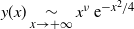 $y(x)\underset{x\rightarrow +\infty}{\sim}x^\nu \,\textrm{e}^{-x^2/4}$. The other independent solution of (A8) is
 $x\mapsto D_\nu({-}x)$.
We have the following relation:
 \begin{equation}\partial_x D_\nu(x)=\nu D_{\nu-1}(x)-\dfrac{x}{2}D_\nu(x).\end{equation}
When Re $(\nu) >-1$,
 \begin{equation}D_\nu(x\sqrt{2})=\dfrac{2^{{{{\nu}/{2}}}+1}\,\textrm{e}^{{{{x^2}/{2}}}}}{\sqrt{\pi}} \int_0^\infty \,\textrm{e}^{-t^2} t^\nu \cos\bigg(2xt-\dfrac{\nu\pi}{2}\bigg) \,\textrm{d} t.\end{equation}
For  $n\in\mathbb{N}$ we have
 \begin{equation}\int_{-\infty}^{0} D_{n}^2 ({-}x\sqrt{2}) \,\textrm{d} x = n! \dfrac{\sqrt{\pi}}{2}.\end{equation}
The parabolic cylinder function and the Hermite function are linked by the following relation:
 \begin{equation*} D_\nu(x\sqrt{2})=2^{-{\nu}/{2}} \,\textrm{e}^{-{x^2}/{2}}H_\nu (x). \end{equation*}
A.2. Useful results
In this subsection we let  $\nu_{\alpha}$ denote a zero of
 $\nu \mapsto D_\nu({-}\alpha\sqrt{2})$. This is equivalent to a zero of
 $\nu \mapsto H_{\nu}({-}\alpha)$.
Thanks to (A5), for  $x\in \mathbb{R}$ and when Re
 $(\nu)>-1$, we have
 \begin{align}\partial_x H_\nu(x)&=2xH_\nu(x) -\dfrac{2\textrm{e}^{x^2}}{\sqrt{\pi}}\int_0^{\infty} \,\textrm{e}^{-t^2} (2t)^{\nu+1} \sin\bigg(2xt-\dfrac{\nu\pi}{2}\bigg) \,\textrm{d} t,\qquad\qquad\qquad\quad\ \ \end{align}
 \begin{align}\partial_\nu H_\nu(x) &=\dfrac{2\textrm{e}^{x^2}}{\sqrt{\pi}}\int_0^{\infty} \,\textrm{e}^{-t^2} (2t)^\nu \bigg[\ln(2t)\cos\bigg(2xt-\dfrac{\nu\pi}{2}\bigg)+\dfrac{\pi}{2} \sin\bigg(2xt-\dfrac{\nu\pi}{2}\bigg)\bigg] \,\textrm{d} t,\end{align}
 \begin{align}\partial_x\partial_\nu H_\nu(x)&=2x\partial_\nu H_\nu(x) \notag\\[4pt]&\quad\, -\dfrac{2\textrm{e}^{x^2}}{\sqrt{\pi}}\int_0^{\infty} \,\textrm{e}^{-t^2} (2t)^{\nu+1} \bigg[\ln(2t)\sin\bigg(2xt-\dfrac{\nu\pi}{2}\bigg)-\dfrac{\pi}{2} \cos\bigg(2xt-\dfrac{\nu\pi}{2}\bigg)\bigg] \,\textrm{d} t.\quad \ \end{align}
Thanks to (A8), we can prove by direct induction that  $x \mapsto D_\nu(x)$ is a
 $\mathcal{C}^{\infty}(\mathbb{R})$ function. Then so is
 $x\mapsto H_\nu(x)$.
With the above expressions we can prove that all the derivatives with respect to  $\nu$ exist and are continuous if
 $\nu\in \mathbb{R}_+$. Then
 $\nu \mapsto H_\nu(x)$ is a
 $\mathcal{C}^{\infty}(\mathbb{R}_+)$ function. The cross partial derivatives with respect to
 $\nu$ and x also exist and are continuous. Then we have the symmetry of second derivatives (Schwarz’s theorem).
Here we give several results useful in the proofs.
Proposition A.1. For all  $\nu,\alpha \in \mathbb{R}$, we have
 \begin{equation*}\int_{-\infty}^\alpha \,\textrm{e}^{-{{{x^2}/{2}}}}D_\nu({-}x\sqrt{2})\,\textrm{d} x=\dfrac{\textrm{e}^{-{{{\alpha^2}/{2}}}}}{\sqrt{2}} D_{\nu-1}({-}\alpha\sqrt{2}).\end{equation*}
Proof. We prove the relation on H. Let us take  $\nu,\alpha \in \mathbb{R}$. We have, with (A3) and (A2),
 \begin{align*}\int_{-\infty}^\alpha \,\textrm{e}^{-x^2}H_{\nu}({-}x)\,\textrm{d} x &= -\int_{-\infty}^\alpha \,\textrm{e}^{-x^2} (2xH_{\nu-1}({-}x)+2(\nu -1) H_{\nu-2}({-}x))\,\textrm{d} x\\[3pt]&=\int_{-\infty}^\alpha \partial_x (\textrm{e}^{-x^2}H_{\nu-1}({-}x))\,\textrm{d} x.\end{align*}
Finally,
 \begin{equation*}\int_{-\infty}^\alpha \,\textrm{e}^{-x^2}H_{\nu}({-}x)\,\textrm{d} x=\textrm{e}^{-\alpha^2}H_{\nu-1}({-}\alpha).\end{equation*}
Proposition A.2. For all  $\alpha \in\mathbb{R}$, we have
 \begin{equation*}\int_{-\infty}^{\alpha} D_{\nu_\alpha }^2({-}x\sqrt{2}) \,\textrm{d} x = -\dfrac{\nu_\alpha }{\sqrt{2}} D_{\nu_\alpha -1} ({-}\alpha\sqrt{2})\partial_\nu D_{\nu_\alpha} ({-}\alpha\sqrt{2}).\end{equation*}
Proof. We apply the method given in [Reference Sleeman19]. Let us set
 \begin{equation*} \raisebox{10pt}{\hbox{${f}\colon\ \ $}}\left|\ \begin{array}{c@{\ \ \ }c@{\ \ \ }c} {\mathbb{R}^2}&\longrightarrow &{\mathbb{R}}\\[3pt] {(\nu,x)}&\longmapsto &{D_\nu ({-}x\sqrt{2}).}\end{array}\right. \end{equation*}
Then, thanks to (A8), the function f is a solution of the following PDE. For all  $\nu,x\in \mathbb{R}$,
 \begin{equation*}\partial^2_{x^2}f(\nu,x)+ ({-}x^2+1+2\nu)f(\nu,x)=0.\end{equation*}
We derive this equation with respect to  $\nu$ and using the regularity of H:
 \begin{equation*}\partial^2_{x^2} \partial_\nu f(\nu,x)+2f(\nu,x)+ ({-}x^2+1+2\nu)\partial_\nu f(\nu,x)=0.\end{equation*}
We multiply by f:
 \begin{equation*}f(\nu,x)\partial^2_{x^2} \partial_\nu f(\nu,x)+2f^2(\nu,x)+ ({-}x^2+1+2\nu)f(\nu,x)\partial_\nu f(\nu,x)=0.\end{equation*}
We integrate with respect to x:
 \begin{align*}\int_{-\infty}^{\alpha} f^2(\nu,x) \,\textrm{d} x &=-\dfrac{1}{2}\bigg[\int_{-\infty}^{\alpha} f(\nu,x)\partial^2_{x^2} \partial_\nu f(\nu,x)\,\textrm{d} x +\int_{-\infty}^{\alpha} ({-}x^2+1+2\nu)f(\nu,x)\partial_\nu f(\nu,x) \,\textrm{d} x\bigg]\\[3pt]&=-\dfrac{1}{2}\bigg[ f(\nu,{\alpha})\partial_{x} \partial_\nu f(\nu,{\alpha})-\int_{-\infty}^{\alpha} \partial_x \bigg\lbrace \partial_x f(\nu,x) \partial_\nu f(\nu,x) \bigg\rbrace \textrm{d} x \bigg]\\[3pt]&=-\dfrac{1}{2} [ f(\nu,{\alpha})\partial_{x} \partial_\nu f(\nu,{\alpha})-\partial_x f(\nu,{\alpha}) \partial_\nu f(\nu,{\alpha}) ].\end{align*}
Then, using the function D, we obtain
 \begin{align*}\int_{-\infty}^{\alpha} D^2_{\nu_\alpha} ({-}x\sqrt{2}) \,\textrm{d} x&=\dfrac{-\sqrt{2}}{2}\partial_x D_{\nu_\alpha }({-}{\alpha}\sqrt{2}) \partial_\nu D_{\nu_\alpha} ({-}{\alpha}\sqrt{2}).\end{align*}
The conclusion follows via (A9).  \hfill$\Box$
Proposition A.3. For all  $\alpha \in \mathbb{R}$, there exists
 $g\colon \alpha\mapsto \nu_\alpha$, continuously differentiable on a neighbourhood of
 $\alpha$. We denote
 $\nu_\alpha'=g'(\alpha)$. Then
 \begin{equation*}\nu^{\prime}_\alpha=\dfrac{\partial_x H_{\nu_\alpha}({-}\alpha)}{\partial_\nu H_{\nu_\alpha}({-}\alpha)}.\end{equation*}
Proof. Set
 \begin{equation*} \raisebox{10pt}{\hbox{${f}\colon \ \ $}}\left|\ \begin{array}{c@{\ \ \ }c@{\ \ \ }c} {\mathbb{R}^2}&\longrightarrow &{\mathbb{R}}\\[3pt] {(\nu,x)}&\longmapsto &{D_\nu ({-}x\sqrt{2}).}\end{array}\right.\end{equation*}
The function f is a continuously differentiable function. We have  $f(\nu_\alpha,\alpha)=0$. We also have
 $\partial_\nu f(\nu_\alpha,\alpha)\neq 0$ because of Proposition A.2. and the fact that
 $\int_{-\infty}^{\alpha} D_{\nu}^2({-}x\sqrt{2}) \,\textrm{d} x\neq 0$.
Then, thanks to the implicit function theorem, there exists an open set U of  $\mathbb{R}$ containing
 $\alpha$ such that there exists a unique continuously differentiable function
 $g\colon U \mapsto \mathbb{R}$ such that
 $g(\alpha)=\nu_\alpha$ and for all
 $x \in U$,
 $f(g(x),x)=0$.
Moreover, the partial derivative of g in U is given by
 \begin{equation*} g'(x)=-\dfrac{\partial_x f(g(x),x)}{\partial_\nu f(g(x),x)}.\tag*{$\Box$}\end{equation*}
Proposition A.4. For all  $m,x \in \mathbb{R}$, we have
 \begin{align*}\partial_m (H_{\nu_m }(x))&=\textrm{e}^{x^2-m^2}\partial_x H_{\nu_m }({-}m)-\dfrac{4\nu^{\prime}_m \,\textrm{e}^{x^2}}{\sqrt{\pi}} \int_0^{\infty}\,\textrm{e}^{-t^2}(2t)^{\nu_m } \sin((m+x)t)\\[3pt] &\quad\, \times \bigg[\ln(2t)\sin\bigg((x-m)t-\dfrac{\nu_m \pi}{2}\bigg)-\dfrac{\pi}{2}\cos\bigg((x-m)t-\dfrac{\nu_m \pi}{2}\bigg)\bigg]\,\textrm{d} t.\end{align*}
Proof. Using Proposition A.3. twice and (A12) and (A13), we have
 \begin{align*}\partial_m (H_{\nu_m }(x))&=\nu^{\prime}_m \partial_\nu H_{\nu_m }(x)\\[3pt]&=\nu^{\prime}_m \partial_\nu H_{\nu_m }(x) + \textrm{e}^{x^2-m^2}\partial_x H_{\nu_m }({-}m) - \textrm{e}^{x^2-m^2}\partial_x H_{\nu_m }({-}m)\\[3pt]&=\nu^{\prime}_m \partial_\nu H_{\nu_m }(x) + \textrm{e}^{x^2-m^2}\partial_x H_{\nu_m }({-}m) - \textrm{e}^{x^2-m^2}\nu^{\prime}_m (\partial_\nu H)_{\nu_m }({-}m)\\[3pt]&=\textrm{e}^{x^2-m^2}\partial_x H_{\nu_m }({-}m)-\dfrac{4\nu^{\prime}_m \,\textrm{e}^{x^2}}{\sqrt{\pi}} \int_0^{\infty} \,\textrm{e}^{-t^2}(2t)^{\nu_m } \sin((m+x)t)\\[3pt] &\quad\, \times\bigg[\ln(2t)\sin\bigg((x-m)t-\dfrac{\nu_m \pi}{2}\bigg)-\dfrac{\pi}{2}\cos\bigg((x-m)t-\dfrac{\nu_m \pi}{2}\bigg)\bigg]\,\textrm{d} t.\tag*{$\Box$}\end{align*}
In particular, with  $x=-m$, we have the following proposition.
Proposition A.5. For all  $m \in \mathbb{R}$, we obtain
 \begin{equation*}\partial_m (H_{\nu_m }(x))|_{x=-m}=\partial_x H_{\nu_m }({-}m).\end{equation*}
We also have the following result.
Proposition A.6. For all  $m \in \mathbb{R}$, we have
 \begin{align*}\partial^2_{m^2} (H_{\nu_m }(x))|_{x=-m}= 2\nu^{\prime}_m\partial_\nu \partial_x H_{\nu_m}({-}m)+2m\partial_x H_{\nu_m}({-}m).\end{align*}
Proof. This is the same kind of calculus as in the proof of Proposition A.4.. We use formula (A14) and the fact that
 \begin{align*}\partial^2_{m^2} (H_{\nu_m }(x))|_{x=-m}&= -2m\partial_x H_{\nu_m}{({-}m)} + \partial_m (\partial_x H_{\nu_m}({-}m))\\[3pt] &\quad\, -\dfrac{2\nu^{\prime}_m \,\textrm{e}^{m^2}}{\sqrt{\pi}} \int_0^\infty \,\textrm{e}^{-t^2} (2t)^{\nu_m+1} \bigg[\ln(2t)\sin (\varsigma_{m}(t))-\dfrac{\pi}{2} \cos (\varsigma_{m}(t))\bigg] \,\textrm{d} t,\end{align*}
where  $\varsigma_{m}(t)\,:\!=-2mt-{{{\nu_m\pi}/{2}}}$.
 \hfill$\Box$
Acknowledgements
We thank Grégory Vial for his comments on this paper.