1. Introduction
Efficient and accurate analysis of traversability is essential for enabling unmanned mobile platforms to attain autonomous navigation. Specifically, autonomous vehicles rely on traversability analysis results, combined with their own capabilities, to plan a safe and reliable path [Reference Waibel, Löw, Nass, Howard, Bandyopadhyay and Borges1–Reference Alamiyan-Harandi, Derhami and Jamshidi3]. In recent years, the need for terrain perception in complex environments has driven traversability analysis to evolve from a binary classification problem into a multi-class problem. Instead of simply distinguishing between passable and impassable areas, traversability is now categorized into several levels based on traversability difficulty.
Most autonomous navigation systems include a traversability analysis module [Reference Jian, Lu, Zhou, Lan, Xiao, Wang and Liang4–Reference Zhou, Yi, Zhang, Chen, Yang, Han and Zhang9], which typically evaluates terrain difficulty by calculating attributes such as slope, terrain roughness, and step height, based on spatial distribution features of point clouds, such as height, variance, and normals. However, while geometric information might suggest that certain obstacles make a path impassable, the robot may actually be able to traverse them, as in the case of grass or leaves. Meanwhile, many researchers [Reference Guan, He, Song and Zhang10,Reference Kim, Seo, Ahn and Kim11] have begun utilizing the rich semantic information provided by visual sensors to study environmental traversability using image segmentation networks like U-Net [Reference Ronneberger, Fischer and Brox12]. However, such methods often map 2D image segmentation results to 3D space based on the relative position between the camera and light detection and ranging (LiDAR), which may lead to inaccurate mapping results due to calibration errors.
Therefore, BEVNet [Reference Shaban, Meng, Lee, Boots and Fox13] proposes a semantic terrain classification framework that voxelizes point clouds in 3D space and employs sparse 3D convolutions for feature extraction, ultimately achieving BEV semantic category prediction. While effective in capturing 3D features, this method faces challenges related to deployment complexity and slow inference speed because of its reliance on computationally expensive 3D convolutions.
To solve above challenges, inspired by BEV-based object detection methods for urban structured environments [Reference Zhou and Tuzel14–Reference Lang, Vora, Caesar, Zhou, Yang and Beijbom16], this paper proposes a real-time terrain traversability classification approach, which achieves an inference speed exceeding 110 FPS. The main contributions are as follows:
-
• We propose a real-time LiDAR-based terrain traversability classification network in off-road environments, achieving fast and dense prediction of terrain traversability around the ego vehicle.
-
• We propose a fast BEV feature map generation method that employs the dynamic voxelization and pillar feature encoding to reduce information loss and improve efficiency.
-
• We propose a traversability completion method with an encoder-decoder architecture that fully leverages sparse BEV features to achieve accurate and dense terrain traversability prediction.
-
• Quantitative and qualitative experiments on RELLIS-3D (off-road) dataset and SemanticKITTI (on-road) dataset are carried out to prove the efficiency and accuracy of proposed approach.
We organize the paper as follows. First of all, Section 2 describes the related work of this paper. Then, the proposed real-time terrain traversability classification approach is introduced in Section 3, with a detailed description of the structural composition in the network. Next, Section 4 presents the implementation details, experimental results, and corresponding analyses. Finally, conclusions and limitations are drawn in Section 5.
2. Related Work
2.1. Point cloud 3D object detection
PointNet [Reference Qi, Su, Mo and Guibas17] introduced an effective solution for directly processing 3D point clouds, using shared multilayer perceptrons to extract features for each point in the cloud, followed by max pooling to capture global features. However, achieving real-time performance in complex 3D scenes while capturing local semantic information poses a significant challenge for point-based methods. Consequently, voxel-based 3D detection and segmentation methods have gained popularity because of the ability to preserve neighborhood structures in the original point cloud efficiently.
VoxelNet [Reference Zhou and Tuzel14] divides point cloud data into voxels and applies multiple PointNet structures within each voxel to extract features. This is followed by 3D convolution to model interactions between voxels, and finally, a region proposal network is used for the 3D detection task. To address the speed limitations of VoxelNet, SECOND [Reference Yan, Mao and Li15] leverages the sparsity of point clouds and proposes 3D sparse convolution, significantly improving both training and inference speeds. PointPillars [Reference Lang, Vora, Caesar, Zhou, Yang and Beijbom16], on the other hand, avoids segmentation along the vertical axis, instead extracting pillar features from the point cloud. This eliminates the need for 3D convolutions, enhancing inference speed and simplifying deployment. Our method builds upon the PointPillars, achieving even higher efficiency while maintaining accuracy.
2.2. 2D semantic segmantation
FCN [Reference Shelhamer, Long and Darrell18] was the first model to successfully apply convolutional neural networks to image segmentation, achieving end-to-end pixel-level prediction. Subsequently, U-Net [Reference Ronneberger, Fischer and Brox12] introduced an encoder-decoder structure with skip connections that fuse features from different layers, effectively preserving multi-scale information and demonstrating excellent performance. DeepLab [Reference Chen, Zhu, Papandreou, Schroff and Adam19] further improved segmentation accuracy by introducing dilated convolution and an atrous spatial pyramid pooling module (ASPP), enhancing the ability of model to handle objects at multiple scales.
In recent years, to meet real-time segmentation requirements in complex scenarios, many researchers have proposed lightweight real-time 2D image segmentation models [Reference Howard, Sandler, Chu, Chen, Chen, Tan, Wang, Zhu, Pang, Vasudevan, Le and Adam20–Reference Fan, Lai, Huang, Wei, Chai, Luo and Wei23]. For example, MobileNet [Reference Howard, Sandler, Chu, Chen, Chen, Tan, Wang, Zhu, Pang, Vasudevan, Le and Adam20] replaces standard convolutions with depthwise separable convolutions to reduce computational cost, with subsequent versions iteratively improving the network structure. BiSeNet [Reference Yu, Wang, Peng, Gao, Yu and Sang21] employs a dual-branch network architecture, where the spatial path extracts spatial information, and the context path uses lightweight models and global average pooling to expand the receptive field, achieving a balance between speed and accuracy.
2.3. Traversability analysis
Existing traversability analysis methods can be distributed into three main classes: methods based on 2D image space, 3D space, and BEV space. Methods based on 2D image space typically formulate traversability analysis problem as a semantic segmentation task [Reference Guan, Kothandaraman, Chandra, Sathyamoorthy, Weerakoon and Manocha2,Reference Min, Jiang, Zhao, Xu, Xiao, Nie and Dai24], employing neural network models to analyze features such as color and texture from images. For instance, ORFD [Reference Min, Jiang, Zhao, Xu, Xiao, Nie and Dai24] employs a transformer-based model for traversable area detection in off-road scenarios, using cross-attention mechanisms to adaptively fuse multimodal information from point clouds and images.
Methods based on 3D space predominantly rely on LiDAR and analyze point cloud geometric features. A representative approach is patchwork [Reference Lim, Oh and Myung25], which utilizes a concentric zone model for non-uniform region segmentation, regional ground plane fitting for ground estimation, and ground likelihood estimation to determine whether a region constitutes actual ground. Shan et al. [Reference Shan, Wang, Englot and Doherty26,Reference Doherty, Shan, Wang and Englot27] addressed the challenge of sparse data in traversable terrain mapping by performing elevation inference and traversability classification for unobserved areas using Bayesian generalized kernel inference. Methods based on BEV space have benefited from the rise of BEV perception frameworks [Reference Li, Wang, Wang and Zhao28–Reference Liu, Tang, Amini, Yang, Mao, Rus and Han30] to model road edges or structures using multi-view camera images or point clouds. HDMapNet [Reference Li, Wang, Wang and Zhao28], for example, performs semantic prediction, instance embedding, and direction prediction with image encoder and view transformer to generate a vectorized representation of roads.
3. Method
As illustrated in Figure 1, the BEV feature map generation module divides point cloud into pillars and extracts pillar features to create BEV feature map. The traversability completion module further processes the BEV feature map using a network module with encoder-decoder structure. Offline data processing is used to generate dense traversability labels. The network classifies the traversability of the observed areas and predicts the traversability of unobserved areas to generate the final traversability map.
Overall architecture of real-time LiDAR-based terrain traversability classification approach.

3.1. BEV feature map generation
Due to the unordered and sparse nature of point clouds, many previous works first perform spatial voxelization in
 $xyz$
dimensions for subsequent processing. However, in this work, to meet the real-time requirements of perception tasks such as autonomous navigation, we divide the point cloud into pillars on the
 $xy$
-plane without any discretization along the
 $z$
-axis, thus eliminating the dependence on 3D convolution. Furthermore, by leveraging fast dynamic voxelization, pillar feature encoding and scatter, the input point cloud is efficiently converted into a BEV feature map, which significantly improves computational efficiency and meets the requirements of the BEV-based traversability prediction task.
3.1.1. Dynamtic voxelization
During the process of voxelization, the hard voxelization method encodes the point clouds into tensor with dimensions
 $(M, Q, C)$
, where
 $M$
denotes the number of pillars which are not empty,
 $Q$
represents the maximum number of points contained within every pillar, and
 $C$
indicates the number of features per point. This method requires pre-allocating a fixed-size tensor and, based on the size of tensor, sampling voxels that exceed the predefined number of points while padding those that fall short, resulting in information loss and increased computational overhead.
In order to tackle this issue, a dynamic voxelization method was proposed by Zhou et al. [Reference Zhou, Sun, Zhang, Anguelov, Gao, Ouyang, Guo, Ngiam and Vasudevan31], which eliminates the need to sample each point cloud into a predefined number of voxels with fixed capacities, such as
 $M$
non-empty voxels and
 $Q$
points per voxel in hard voxelization. Instead, it maintains a complete mapping between points and voxels:
 \begin{equation} \begin{aligned} & M_P(v_i)=\{ p_j|\forall {p_j}\in v_i \}, \forall {i} ,\\ & M_V(p_j)=v_i,\forall {j} , \end{aligned} \end{equation}
where
 $v_i$
and
 $p_j$
represent voxel and point, respectively, and
 $M_P(v_i)$
and
 $M_V(p_j)$
create bi-directional connections within each pair of
 $v_i$
and
 $p_j$
. The number of nonzero voxels in 3D space and the number of points in each voxel dynamically vary based on the input point cloud. This adaptive allocation eliminates the requirement for a fixed-size tensor and mitigates information loss caused by random point or voxel dropout, thereby enhancing both computational efficiency and overall performance.
For example, for a point cloud of size
 $(120000, 4)$
, to minimize information loss while reducing memory overhead, following the experience from PointPillars [Reference Lang, Vora, Caesar, Zhou, Yang and Beijbom16], the hard voxelization method can be configured with a maximum number of pillars M = 20,000 and a maximum number of points per pillar Q = 64. This results in allocating a buffer of size
 $(20000, 64, 4)$
for subsequent feature encoding. If the number of pillars exceeds 20,000 or the number of points per pillar exceeds 64, downsampling is applied to meet the predefined constraints. If the number of points in a pillar is less than 64, zero-padding is performed to maintain tensor shape consistency. Since
 $20000 \times 64 \gt 120000$
, meaning the theoretically allocated storage significantly exceeds the actual number of points, this may introduce redundant memory overhead, leading to increased memory consumption.
Specifically, the input to the BEV feature map generation module is a single frame of point cloud with a dimension of
 $(N, 5)$
, where
 $N$
denotes the number of points. Each point is represented as
 $p = [b, x, y, z, r]$
, where
 $b$
indicates the batch index,
 $[x, y, z]$
are the coordinates of the point, and
 $r$
denotes its reflectance intensity. The point cloud is then discretized into an evenly spaced grid on the
 $xy$
-plane, forming a set of vertical columns known as pillars. The corresponding discrete grid indices are computed as:
 \begin{equation} \begin{aligned} (i_x, i_y) = \left ( \left \lfloor \frac {x - x_{\min }}{v_x} \right \rfloor , \left \lfloor \frac {y - y_{\min }}{v_y} \right \rfloor \right ), \end{aligned} \end{equation}
where
 $(v_x, v_y)$
denotes the grid resolution along the X and Y axes,
 $(x_{\min }, y_{\min })$
represents the lower bounds of the point cloud range, and the floor operator
 $\lfloor \cdot \rfloor$
indicates rounding down to the nearest integer. To support batched processing, a unique grid index is constructed for each point based on its batch index and grid index as:
 \begin{equation} \begin{aligned} id = b \times S_{xy} + i_x \times S_y + i_y, \end{aligned} \end{equation}
where
 $S_{xy} = H \times W$
is the total number of grid cells per batch (i.e., the product of the grid’s height and width), and
 $S_y = H$
is the height of the grid. Using this flattened encoding, all points assigned to the same grid cell share the same
 $id$
. The function
 $torch.unique$
is then applied to extract the set of unique grid indices along with the inverse mapping, enabling subsequent pillar-wise feature encoding and scattering onto the
 $xy$
-plane.
3.1.2. Pillar feature encoding and scatter
Data augmentation is first applied to each point
 $p = [x, y, z, r]$
, where
 $[x, y, z]$
represents the real coordinates of the point, and
 $r$
denotes its reflectance intensity. Specifically, we enhance the point features to
 $p = [x, y, z, r, x_n, y_n, z_n, x_s, y_s, z_s]$
, where
 $[x_n, y_n, z_n]$
represents the offset from the mean coordinates of all points within the corresponding pillar, and
 $[x_s, y_s, z_s]$
denotes the offset from the geometric center of the pillar. The inclusion of
 $[z_s]$
in particular helps compensate for the potential loss of vertical structure information along the Z-axis. The augmented point cloud tensor
 $(N, 10)$
is then processed by a simplified PointNet model, which consists of a Linear layer, a Batch Normalization layer, and a ReLU activation function, to extract high-level features for every point, resulting in a feature tensor
 $(N, C)$
.
Based on the mapping between points and pillars, we perform max-pooling on the points within the same pillar to retain the most representative feature information for that pillar, yielding a pillar feature tensor
 $(M, C)$
. Finally, the pillar features are scattered onto the BEV plane according to the spatial coordinates of the pillars within the BEV grid, generating a BEV feature map
 $T(H, W, C)$
, where each pixel stores the pillar features corresponding to that location.
3.2. Traversability completion
After generating the BEV feature map
 $T$
, it is necessary to classify the traversability of each grid cell within the BEV map based on the extracted BEV features, and at the same time to predict the traversability of grid cells that lack features, i.e., unobserved grid cells, to ultimately produce a dense BEV traversability map. In order to achieve dense, pixel-level prediction of terrain traversability around the ego vehicle while maintaining real-time performance, we propose a traversability completion module inspired by the real-time image semantic segmentation network PP-LiteSeg [Reference Peng, Liu, Tang, Hao, Chu, Chen, Wu, Chen, Yu, Du, Dang, Lai, Liu, Hu, Yu and Ma22]. Figure 2(a) is the overall architecture of the traversability completion module.
The input to the traversability completion module is the BEV feature map
 $T$
. Firstly, STDCBackbone [Reference Fan, Lai, Huang, Wei, Chai, Luo and Wei23] is used as the encoder, which is structured into five stages. The first and second stages utilize
 $3\times 3$
convolutions to downsample the input feature map, producing a feature map at
 $\frac {1}{4}$
resolution. The third to fifth stages incorporate Short-Term Dense Concatenation (STDC) modules, progressively producing feature maps at
 $\frac {1}{8}$
,
 $\frac {1}{16}$
, and
 $\frac {1}{32}$
resolutions, respectively. The structure of the STDC module is illustrated in Figure 2(b), where the left and right sides represent STDC modules with stride of 2 and stride of 1, respectively. Each stage begins with an STDC module with stride of 2 for downsampling, followed by several STDC modules with stride of 1, which preserves the feature map size while enhancing feature extraction. To better adapt the encoder to the BEV-based traversability classification task and mitigate potential information loss caused by early-stage channel reduction, we refine the channel configuration of the encoder to [64, 128, 256, 512, 1024].
(a) is the overall architecture of the traversability completion module. (b)–(d) are the architecture for each component within the traversability completion module. ConvX represents Conv + BN + ReLU, AP represents average pooling.

To further expand the receptive field, we employ the Spatial Pyramid Pooling Module, as illustrated in Figure 2(c). First, adaptive average pooling is applied to the
 $\frac {1}{32}$
resolution feature map from the encoder, generating pooled feature maps of sizes
 $1\times 1$
,
 $2\times 2$
, and
 $4\times 4$
. These pooled features are then processed by
 $1\times 1$
convolutions and upsampled to restore their original size. Finally, the feature maps are summed and passed through a
 $3\times 3$
convolution layer, producing refined features enriched with global contextual information.
To fully exploit the advantages of multi-scale features, we employ the Unified Attention Fusion Module, as illustrated in Figure 2(d). First, a
 $1\times 1$
convolution is applied to reduce the number of channels and enhance the discriminability of low-level features, while high-level features are upsampled to match the spatial size of the low-level features. To fully utilize the detailed information of low-level features and the global information of high-level features, a spatial attention mechanism is introduced to generate adaptive weighting coefficients
 $\alpha$
, which guide the fusion of low-level and high-level features, enhancing feature representation. The fusion process is formulated as follows:
 \begin{equation} \begin{aligned} & \alpha = Sigmoid(Conv(Cat(Avg(F_{low}),Max(F_{low}),Avg(F_{high}),Max(F_{high})))),\\ & F = (1-\alpha )F_{low}+\alpha F_{high} , \end{aligned} \end{equation}
Finally, a
 $3\times 3$
convolution is applied to improve spatial coherence and reduce the channel dimension to the number of target classes. The feature map is then progressively upsampled to the desired resolution to generate the predicted traversability map.
3.3. Traversability dataset construction
Similar to BEVNet, we perform offline data processing on the RELLIS-3D [Reference Jiang, Osteen, Wigness and Saripalli32] off-road dataset and SemanticKITTI on-road dataset. The required data include point cloud data, point cloud semantic labels, and poses of each scan. Firstly, we aggregate the point clouds from the previous
 $t$
frames and the subsequent
 $t$
frames for each frame of point clouds, utilizing the inter-frame pose data with an interval step size
 $s$
, to make the data denser and more accurate. We classify the points into static points and potentially dynamic points based on their semantic labels. Specifically, in the SemanticKITTI dataset, we consider points labeled as “moving” as dynamic points, while in the RELLIS-3D dataset, we consider points labeled as “person” as dynamic points. In order to avoid ghosting of dynamic objects during the aggregation process, we remove dynamic points from frames other than the current frame.
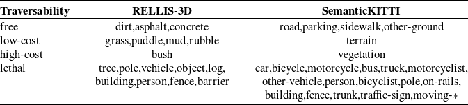
Mapping of semantic-traversability labels.

Visualization of BEV traversability datasets RELLIS-3D (off-road) and SemanticKITTI (on-road). (a) RGB images are shown for visualization purposes only.

Subsequently, we map all semantic labels of the points into four traversability cost labels: free, low-cost, high-cost, and lethal, as shown in Table I. For example, roads or concrete with minimal resistance are categorized as free. Terrain or grass, where vehicles can pass but may encounter resistance or bumps, is classified as low-cost. Vegetation or bush that makes vehicle traversal difficult is labeled as high-cost, while categories prone to hazards, such as trees and cars, are classified as lethal. Finally, the points are projected onto the
 $xy$
-plane, and the traversability category for each grid cell is determined based on the highest traversability cost label among all points falling within that cell. Grid cells that do not contain any projected points are assigned an additional class label unknown. The resulting
 $xy$
-plane, where each grid cell stores a traversability label, serves as the dense ground truth traversability map. We set the size of the traversability map to a range of 51.2m from the front, back, left, and right of the vehicle, with a resolution of 0.2m. Figure 3 shows the visualization of datasets, where RGB images are used solely for visualization and are not utilized in the network.
4. Experiments
4.1. Implementation details
In this section, we conduct quantitative and qualitative experiments on the RELLIS-3D off-road dataset and the SemanticKITTI on-road dataset. The RELLIS-3D dataset is collected using a Clearpath Robotics Warthog platform, equipped with a 64-channel Ouster OS1 LiDAR for off-road perception, along with a GPS and inertial navigation system for precise pose estimation. The SemanticKITTI dataset is captured from a vehicle equipped with a Velodyne HDL-64E LiDAR and a GPS/IMU system, primarily for on-road perception and navigation.
To obtain dense ground truth labels, consistent with BEVNet,
 $t=70$
and
 $s=5$
for RELLIS-3D, while
 $t=35$
and
 $s=2$
for SemanticKITTI. The traversability map remains consistently centered on the position of the vehicle and is color-coded to indicate different traversability costs: green for free, yellow for low-cost, blue for high-cost, and red for lethal, as shown in Figure 3c. The unknown category is involved in the calculation of losses during the training process, but is not taken into account when evaluating overall accuracy. The number of channels
 $C$
of the BEV feature map
 $T$
is set to 64, and the Adam optimizer is used with a learning rate of
 $lr = 3.0 \times 10^{-4}$
. We employ the cross-entropy loss between the ground truth labels and the predicted results as the objective function to supervise network training. The RELLIS-3D dataset consists of five sequences, with sequence 4 designated as the test sequence and the rest as training sequences. The SemanticKITTI dataset consists of 11 sequences, where sequence 8 is used as the test sequence, and the remaining sequences are used for training.
We compare the proposed method with BEVNet [Reference Shaban, Meng, Lee, Boots and Fox13] and FASTC [Reference Chen, Wei, Liu, Wang, Yang and Liu33], both of which are LiDAR-based terrain traversability classification methods. To ensure fairness, the range of point clouds is uniformly set to
 $\left [(-51.2,51.2),(-51.2,51.2), (-2,1)\right ]$
, and during training, only single-frame point clouds are employed as the network input. All methods are re-trained and evaluated, with both training and inference conducted on a single GeForce RTX 4090 GPU. BEVNet divides the 3D space into a
 $512\times 512\times 30$
grid with a voxel size of
 $\left [ 0.2,0.2,0.1 \right ]m$
, setting the maximum number of points per voxel to 5. It then extracts voxel features using 3D sparse convolution and compresses them into the BEV plane, followed by FCHardNet [Reference Chao, Kao, Ruan, Huang and Lin34] as the inpainting network for traversability classification. FASTC adopts a hard voxelization approach, dividing the 3D space into a
 $512\times 512\times 1$
grid with a pillar size of
 $\left [ 0.2,0.2,3 \right ]m$
and setting the maximum number of points per pillar to 55. It then extracts pillar features using PointNet with a point feature dimension of
 $C=128$
, and employs RegSeg [Reference Gao35] as the completion network for traversability classification.
4.2. Results
4.2.1. Quantitative and qualitative experiments
Quantitative experiments: To assess the accuracy of the network, we use mIoU (mean Intersection over Union) and mAcc (mean Accuracy) as metrics. The formulas are presented below:
 \begin{equation} \begin{aligned} & mIoU = \frac {1}{c} \sum _{i=1}^{c} \frac {TP_i}{TP_i + FP_i + FN_i} ,\\ & mAcc = \frac {1}{c} \sum _{i=1}^{c} \frac {TP_i}{TP_i + FP_i} , \end{aligned} \end{equation}
where
 $TP_i$
,
 $FP_i$
, and
 $FN_i$
, respectively, represent true positives, false positives, and false negatives for the
 $i$
-th traversability cost category.
 $c$
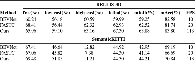
signifies the count of traversable categories. In order to provide a more intuitive comparison of the real-time performance of different methods, we consider the inference speed as a performance metric, measured in frames per second (FPS). The results of the experiment are shown in Table II. In addition, we compute the classification accuracy for each pixel in each image on both the RELLIS-3D and SemanticKITTI datasets, and generate the confusion matrix presented in Figure 4.
Comparison of quantitative experiment results.

Confusion matrix.

It is evident that, on the RELLIS-3D dataset, our method improves the IoU for the four traversability categories by 5.72%, 2.92%, 2.57%, and 7.31%, respectively, compared with BEVNet. Overall, it increases the mIoU by 4.63% and mAcc by 1.22%, while also boosting inference speed by over 11 times. Compared with FASTC, our method improves IoU by 2.66%, 0.84%, and 4.37% in the low-cost, high-cost, and lethal categories, respectively, while experiencing a 2.45% decrease in the free category. This may be attributed to FASTC’s superior ability to learn relatively flat terrains in wild environments, whereas our approach effectively balances predictions across multiple categories. Overall, our method improves mIoU by 1.36% and mAcc by 2.06%, while achieving a fivefold increase in FPS.
On the SemanticKITTI dataset, our method improved the IoU by 2.07% and 5.21% in the free and low-cost categories, respectively, but slightly decreased by 1.61% and 0.62% in the high-cost and lethal categories compared with BEVNet. This may be because, despite the feature augmentation and encoding applied to the point cloud within pillars in our method, the use of spatial voxelization in
 $xyz$
dimensions and 3D convolution allows BEVNet to more effectively capture height-dimensional features. As a result, it achieves better classification performance for higher-cost objects. Overall, it increased by 1.26% on mIoU and 1.65% on mAcc, while also boosting inference speed by over 11 times compared with BEVNet. Compared with FASTC, our method improves IoU by 2.42%, 6.03%, and 3.83% in the free, low-cost, and high-cost categories, respectively, while achieving comparable performance in the lethal category. Overall, our method increases mIoU by 3.07% and mAcc by 4.15%, while achieving a fivefold improvement in FPS.
These results indicate that the dynamic voxelization method significantly reduces preprocessing time by avoiding memory allocation for a fixed-size voxel grid. It preserves a complete mapping between points and voxels and enables direct operations such as feature extraction on the raw point cloud. This is critical for maintaining real-time performance in off-road environments, where the density and distribution of point clouds can vary significantly. Pillar-based feature encoding eliminates the need for discretization along the
 $z$
-axis and reduces the computational cost associated with 3D convolutions. By discretizing the 3D point cloud into an evenly spaced grid on the
 $xy$
-plane, which forms a set of vertical columns known as pillars, enhancing point features within each pillar, and subsequently extracting pillar features using PointNet, we preserve the essential spatial information while significantly reducing computation time. The real-time traversability completion network adopts an encoder-decoder architecture, which effectively leverages BEV features to generate dense and accurate traversability predictions with low latency, ensuring that the system meets real-time requirements, making it suitable for time-sensitive applications such as autonomous navigation. In summary, these components collectively form a cohesive pipeline that balances accuracy and efficiency for real-time terrain traversability prediction in both off-road and on-road environments.
Comparison of qualitative experiment results.

Qualitative experiments: To more intuitively compare the traversability classification results, we select several instances from validation sequence on both RELLIS-3D off-road dataset and SemanticKITTI on-road dataset for visualization, as shown in Figure 5. Due to the limited sensing range of the LiDAR and occlusion from nearby objects, points become extremely sparse in areas far from the sensor, making it necessary to predict the traversability of those regions based on the surrounding environment. It can be observed that the proposed method is generally more effective in achieving traversability classification and predicting the traversability of unknown areas, with more stable results. In RELLIS-3D, the method effectively distinguishes large high-cost or lethal-cost areas and maintains stable performance even on rugged terrains. In SemanticKITTI, the proposed method effectively differentiates road surfaces and accurately detects both static and dynamic vehicles on the road, achieving satisfactory classification performance.
However, it can also be observed that our method may exhibit instability in detecting small objects, such as pedestrians and traffic lights in the SemanticKITTI dataset, or certain obstacle classes in RELLIS-3D. The primary reason is that these objects typically generate only a few LiDAR returns, resulting in insufficient feature points for reliable classification. Additionally, due to the resolution setting of the BEV space, such small objects occupy only a limited number of pixels and appear sparsely distributed. As a result, the completion network may overlook their features during downsampling, leading to misclassification into surrounding categories. Moreover, for large-scale unknown or occluded regions in the environment, the limited availability of feature points poses a significant challenge for accurate classification. This is especially evident for high-cost classes in the SemanticKITTI dataset, which are often located at the periphery of the road, far from the ego vehicle, and heavily occluded. In these regions, the network must rely on contextual information from nearby points to make predictions, often resulting in lower classification accuracy. Furthermore, the complex structure and relatively small size of the RELLIS-3D dataset can lead to poor generalization in off-road environments. During testing, the network may encounter scene patterns or point distributions that were underrepresented during training, resulting in reduced classification performance. This highlights the need to construct larger and more diverse off-road datasets to improve generalization capability of the model.
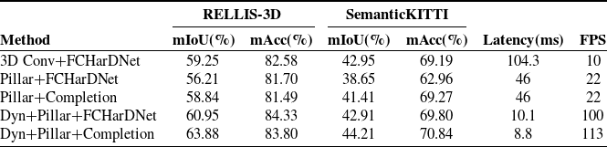
Comparison of ablation study results.

4.2.2. Ablation studies
Analysis of module performance: Table III shows the results of the ablation experiments for each module on RELLIS-3D and SemanticKITTI datasets. Latency refers to the time consumed in processing a single frame of point cloud. Based on BEVNet, we progressively replace its voxelization, feature extraction, and traversability inpainting components. Meanwhile, we compare dynamic voxelization with hard voxelization, with the inpainting module kept unchanged. We set the dimension of the pillar to
 $\left [ 0.2,0.2,3 \right ]$
and the maximum number of points contained in each pillar to 64.
From the first two lines, it can be seen that replacing the voxel representation of the point clouds with the pillar representation can double the inference speed, but it leads to a decrease in the classification accuracy, probably because 3D convolution can extract spatial features more effectively from the point cloud, while pillar-based methods can suffer information loss due to point cloud downsampling and a relatively simple BEV feature extraction approach. Then, the replacement of FCHardNet with our traversability completion module improves the mIoU by 2.63% on RELLIS-3D and 2.76% on SemanticKITTI. Furthermore, the use of dynamic voxelization not only achieves a significant improvement in speed but also enhances mIoU by 4.74% on RELLIS-3D and 4.26% on SemanticKITTI compared with the Pillar + FCHarDNet approach. Finally, by combining dynamic voxelization with traversability completion, mIoU improves by 5.04% on RELLIS-3D and 2.8% on SemanticKITTI compared with Pillar + Completion, achieving a balance between speed and accuracy.
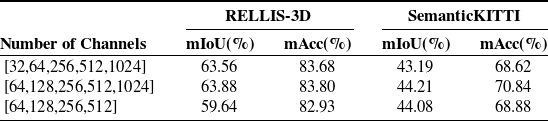
Analysis of model parameter settings: We conducted an analysis of the channel configuration in the encoder of the traversability completion module, as shown in the Table IV. From the first two rows of the table, we can observe that, unlike conventional image segmentation tasks where the input is typically a 3-channel RGB image, this module takes a high-dimensional 64-channel BEV feature map as input. As a result, using a small number of channels (e.g., 32) in the early stages may lead to a loss in overall accuracy due to the insufficient capacity to capture rich feature information. From the last two rows of the table, we can see that for the traversability completion task, using more channels in the later stages of BEV feature encoding enables better extraction of global context, which can be effectively fused with local features during decoding, thereby improving the final accuracy.
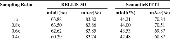
Analysis of point cloud density: To evaluate the impact of point cloud density on classification accuracy, we applied a random subsampling strategy to the point cloud, retaining 80% (0.8x), 60% (0.6x), and 40% (0.4x) of the original points, respectively. The results obtained from different sampling ratios are summarized in Table V, which means that the density of the input point cloud can impact accuracy. A higher point cloud density provides more detailed information, which can improve the precision of traversability classification. Conversely, a lower density may lead to missing details, increasing ambiguity in classification, and potentially reducing accuracy.
5. Conclusions
We propose a real-time LiDAR-based terrain traversability classification approach in off-road environments, achieving accurate and dense predictions of BEV traversability centered on the vehicle. The fast BEV feature map generation module significantly improves training and inference speed, and the traversability completion module enables accurate and dense prediction of four levels of terrain traversability difficulty, supporting fine-grained understanding of the surrounding environment. Experiment results on both RELLIS-3D off-road dataset and SemanticKITTI on-road dataset demonstrate that compared with BEVNet, our method achieves over 11 times improvement in speed while maintaining or even improving accuracy. Nevertheless, the inherently data-driven nature of learning-based methods imposes certain limitations on their generalization capability. For example, the model may need additional fine-tuning when faced with environmental features, such as deep pits, that were not included in the training dataset. We aim to continue working toward solutions for these issues in the future.
Impact of model parameters settings on classification accuracy.

Impact of point cloud density on classification accuracy.

Author contributions
Siyao Wu, Shiyong Zhang, Runhua Wang, and Xijun Zhao designed the approach and conducted the code implementation. Siyao Wu, Shiyong Zhang, and Zhenshuo Liang conducted the experiment comparisons and data gathering. Siyao Wu, Shiyong Zhang, and Xuebo Zhang wrote the article.
Financial support
This work was supported in part by the National Natural Science Foundation of China under Grant 62303249, in part by Beijing Tianjin Hebei Basic Research Cooperation Special Project under Grant 24JCZXJC00390, and in part by the Fundamental Research Funds for the Central Universities.
Competing interests
The authors declare that no conflicts of interest exist.
Ethical approval
Not applicable.
Supplementary material
The supplementary material for this article can be found at https://doi.org/10.1017/S0263574725102324.