


Impact Statement
Land surface temperature (LST) is an important input for estimating evapotranspiration, a central quantity in agriculture. We develop a statistical method for downscaling the blurry but frequent LST data from NASA’s ECOSTRESS mission to a finer scale, using high-resolution imagery from the Landsat satellite, both to delineate agricultural fields and to sharpen the LST estimates within them. By modeling each field as an independent unit, our method remains computationally tractable and provides principled uncertainty quantification, with potential applications in agriculture, urban planning, and climate science.
1. Introduction
Obtaining high-resolution estimates of land surface temperature (LST) given observations from remote sensing satellites is an important problem in environmental statistics; for instance, accurate estimation of LST is crucial for understanding the evapotranspiration (ET), a central quantity in Earth’s water cycle (Fisher et al., Reference Fisher, Melton, Middleton, Hain, Anderson, Allen, McCabe, Hook, Baldocchi, Townsend, Kilic, Tu, Miralles, Perret, Lagouarde, Waliser, Purdy, French, Schimel, Famiglietti, Stephens and Wood2017). Spatial modeling is also used in this context for gap-filling between observed data, but we do not focus on this application in this work. Current attempts to build statistical models for LST data have not been able to sufficiently account for the complex spatial structure of the data, especially around agricultural fields where estimates of LST are most crucial. Traditional spatial models, such as stationary Gaussian processes, fail to capture the abrupt changes in LST that occur at the boundaries of agricultural fields, which can lead to oversmoothing and inaccurate predictions (Paciorek and Schervish, Reference Paciorek and Schervish2006; Kumar and Chakraborty, Reference Kumar and Chakraborty2026). Therefore, there is a need for more sophisticated statistical methods that can effectively model the spatial structure present in LST data.
ET is the sum of evaporation and plant transpiration from the Earth’s land surface to the atmosphere (Fisher et al., Reference Fisher, Melton, Middleton, Hain, Anderson, Allen, McCabe, Hook, Baldocchi, Townsend, Kilic, Tu, Miralles, Perret, Lagouarde, Waliser, Purdy, French, Schimel, Famiglietti, Stephens and Wood2017). It is a key component of the water cycle and is a critical variable in the study of climate change, agriculture, and water resource management. ET is influenced by several factors, including LST, solar radiation, wind speed, and humidity. In particular, LST is a key driver of ET as it controls the amount of energy available for evaporation and transpiration. Accurate estimation of LST is therefore essential for predicting ET.
The ECOsystem Spaceborne Thermal Radiometer Experiment on Space Station (ECOSTRESS) radiometer was deployed on the International Space Station (ISS) in June 2018 to measure LST and emissivity, using an infrared sensor (Fisher et al., Reference Fisher, Lee, Purdy, Halverson, Dohlen, Cawse-Nicholson, Wang, Anderson, Aragon, Arain, Baldocchi, Baker, Barral, Bernacchi, Bernhofer, Biraud, Bohrer, Brunsell, Cappelaere, Castro-Contreras, Chun, Conrad, Cremonese, Demarty, Desai, De Ligne, Foltýnová, Goulden, Griffis, Grünwald, Johnson, Kang, Kelbe, Kowalska, Lim, Maïnassara, McCabe, Missik, Mohanty, Moore, Morillas, Morrison, Munger, Posse, Richardson, Russell, Ryu, Sanchez-Azofeifa, Schmidt, Schwartz, Sharp, Šigut, Tang, Hulley, Anderson, Hain, French, Wood and Hook2020). The overpass return frequency, or revisit rate, of a sensor is the frequency with which that sensor passes over a given location on Earth. The ECOSTRESS mission has a variable overpass return frequency (between 1 and 5 days) and currently provides the highest spatial resolution spaceborne estimates of LST at ~70 m resolution. However, the effective resolution of LST images from ECOSTRESS has been shown to be significantly lower in practice (Holmes et al., Reference Holmes, Poulter, McCorkel, Jennings, Wu, Efremova, Shiklomanov, Johnson, Jhabvala and Hook2024), likely due to blur and artifacts resulting from sensor damage.
The Landsat program is a series of Earth-observing satellite missions jointly managed by NASA and the US Geological Survey (USGS) that has been providing high-resolution imagery of the Earth’s surface since 1972 (Roy et al., Reference Roy, Wulder, Loveland, C.E, Allen, Anderson, Helder, Irons, Johnson, Kennedy, Scambos, Schaaf, Schott, Sheng, Vermote, Belward, Bindschadler, Cohen, Gao, Hipple, Hostert, Huntington, Justice, Kilic, Kovalskyy, Lee, Lymburner, Masek, McCorkel, Shuai, Trezza, Vogelmann, Wynne and Zhu2014). Landsat satellites are equipped with sensors that capture data in multiple spectral bands, including visible, near-infrared, and thermal infrared, allowing for detailed analysis of land cover, vegetation health, and surface temperature. Landsat 8/9 instruments provide data in the visible to shortwave infrared (VSWIR) at a higher resolution (30 m) than ECOSTRESS, but with a lower overpass return frequency (16 days). Landsat 8/9 Thermal Infrared Sensors (TIRS) have fewer thermal bands than ECOSTRESS, resulting in potentially lower fidelity estimates of LST, and are at nominally lower spatial resolution (100 m).
In our work, we leverage the higher-resolution Landsat 8/9 VSWIR data as a proxy for modeling the agricultural field structure present in the ECOSTRESS LST data. This task, often referred to as data fusion, is of broad interest in the remote sensing community, in far more general settings than just LST data (Khaleghi et al., Reference Khaleghi, Khamis, Karray and Razavi2013; Samadzadegan et al., Reference Samadzadegan, Toosi and Dadrass Javan2025). We plot sample images from both missions in Figure 1, which reflects the type of agricultural field structure that is the focus of our work. Note that the ECOSTRESS and Landsat images are not in the same units and are not taken at the same time; this figure is only meant to illustrate the difference in spatial resolution.
Comparison of resolution between ECOSTRESS and Landsat missions over the Salton Sea region in southern California.

Figure 1. Long description
Two-panel satellite imagery comparison.
Panel a, on the left, is labeled E C O S T R E S S with 70 m resolution. The map uses a high-contrast color scale with bright yellows, greens, and dark purples. The Salton Sea is a large, elongated body of water oriented Northwest to Southeast. To the Southeast of the sea, agricultural fields appear as a dense, pixelated grid of dark purple and green squares. The surrounding mountainous terrain to the North and West is rendered in bright yellow and green, showing coarse thermal or spectral detail.
Panel b, on the right, is labeled Landsat with 30 m resolution. This map uses a more uniform teal and dark blue color palette. The Salton Sea appears as a solid dark blue shape. The agricultural grid to the Southeast is significantly sharper and more defined than in the first panel, with individual field boundaries clearly visible. The topographical features of the surrounding mountains are rendered with finer texture and smoother gradients, reflecting the higher spatial resolution of the 30 m data.
There is a long line of work studying downscaling procedures for land surface temperature data by direct regression of the high-resolution images on their low-resolution counterparts using random forest regression (Hutengs and Vohland, Reference Hutengs and Vohland2016; Li et al., Reference Li, Ni, Li and Wu2018; Njuki et al., Reference Njuki, Mannaerts and Su2020) and neural networks (Bindhu et al., Reference Bindhu, Narasimhan and Sudheer2013; Wu et al., Reference Wu, Xia, Chan, Awange and Zhong2022; Li et al., Reference Li, Wan, Yu and Wang2025). By contrast, our statistical approach using Gaussian process regression is new in this literature. Some key advantages of our approach are the better interpretability of the underlying statistical model, weaker modeling assumptions, which may improve robustness, and the ability to obtain principled uncertainties for the resulting reconstruction.
More similar to our approach, Garrigues et al. (Reference Garrigues, Allard and Baret2007) proposed the mosaic process model for block-structured spatial data, which allows for different covariance structures in different regions of the spatial domain. However, the complexity of their model makes it difficult to scale to larger datasets, such as those encountered in remote sensing applications. Their model is also restricted to blocks that are bounded by straight lines through the spatial domain, which is not ideal for modeling agricultural fields with irregular shapes. Furthermore, the tessellation in the mosaic process model is random, which may lead it to be underconstrained for spatial mapping.
Our main contributions in this work are as follows:
-
• We propose a novel statistical method for downscaling LST data from the ECOSTRESS mission using high-resolution data from the Landsat mission as a proxy for modeling agricultural field structure.
-
• We develop a block-diagonal Gaussian process (BDGP) model that captures the spatial structure of the agricultural fields and leverages independence of LST across fields for computational tractability.
-
• We demonstrate the practicality of the proposed method in producing high-resolution LST estimates along with uncertainty quantification.
We outline our methodology in Section 2; the edge detection method is described in Section 2.1, the Fourier regression approach for modeling the mean function is described in Section 2.2, the parameter estimation procedure is described in Section 2.3, and the kriging and uncertainty quantification method is described in Section 2.4. We present our results in Section 3 and conclude with a discussion in Section 4.
2. Methods
It is common to model spatial data using a Gaussian process (GP) (Gelfand et al., Reference Gelfand, Diggle, Guttorp and Fuentes2010). In order to account for the agricultural field structure present in LST data, we model LST using a block-diagonal Gaussian process with a squared exponential kernel. Suppose we have a partition,
$ \mathcal{R}\hskip0.5em := \hskip0.5em \{{R}_1,\dots, {R}_N\} $
 , of
$ \mathcal{X} $
 into
$ N $
 regions. Given a variance parameter
$ \boldsymbol{\sigma} \hskip0.5em := \hskip0.5em \left({\sigma}_1,\dots, {\sigma}_N\right)\in {\left(0,\infty \right)}^N $
 and length scale parameter
$ \mathbf{\ell}\hskip0.5em := \hskip0.5em \left({\mathrm{\ell}}_1,\dots, {\mathrm{\ell}}_N\right)\in {\left(0,\infty \right)}^N $
 , we define the block-diagonal squared exponential covariance kernel with parameters
$ \left(\boldsymbol{\sigma}, \mathbf{\ell}\right) $
 as
$ k\left(x,{x}^{\prime}\right)={\sum}_{r=1}^N{k}_r\left(x,{x}^{\prime}\right) $
 where:

This kernel is stationary within each region. Given any mean function
$ \mu :\mathcal{X}\to \mathrm{\mathbb{R}} $
 , we say that a block diagonal Gaussian process with parameters
$ \left(\mu, \boldsymbol{\sigma}, \mathbf{\ell},\mathcal{R}\right) $
 (denoted
$ \mathrm{BDGP}\left(\mu, \boldsymbol{\sigma}, \mathbf{\ell},\mathcal{R}\right) $
 ) is a GP with a mean function
$ \mu $
 and covariance kernel
$ k $
 of the form above.
We assume that at a given time, the underlying LST field is a BDGP
$ {f}^{\mathrm{ES}}\hskip0.5em := \hskip0.5em \mathrm{BDGP}\left({\boldsymbol{\mu}}^{\mathrm{ES}},{\boldsymbol{\sigma}}^{\mathrm{ES}},{\mathbf{\ell}}^{\mathrm{ES}},\mathcal{R}\right) $
 and that we observe samples from the blurry
$ {\tilde{f}}^{\mathrm{ES}}:= \left({f}^{\mathrm{ES}}\ast {\kappa}_{\mathrm{blur}}\right)+{f}_{\mathrm{sensor}} $
 , where
$ \ast $
 denotes a two-dimensional convolution. Here,
$ {\kappa}_{\mathrm{blur}} $
 is the density of
$ \mathcal{N}\left(0,{\sigma}_{\mathrm{blur}}^2\hskip0.1em I\right) $
 (accounting for the change of support caused by the finite resolution of ECOSTRESS) and
$ {f}_{\mathrm{sensor}}\sim \mathcal{N}\left(0,{\sigma}_{\mathrm{sensor}}^2\hskip0.1em I\right) $
 accounts for sensor noise within ECOSTRESS. We further assume that the Landsat data are generated from
$ {f}^{\mathrm{LS}}\hskip0.5em := \hskip0.5em \mathrm{BDGP}\left({\boldsymbol{\mu}}^{\mathrm{LS}},{\boldsymbol{\sigma}}^{\mathrm{LS}},{\mathbf{\ell}}^{\mathrm{LS}},\mathcal{R}\right) $
 . We make the simplifying assumption that
$ {\mathbf{\ell}}^{\mathrm{ES}}={\mathbf{\ell}}^{\mathrm{LS}} $
 in order to ensure that the parameters are identifiable in this model.
Then, we outline our LST downscaling procedure as follows:
-
(1) Edge detection: Use edge detection methods on an averaged high-resolution Landsat image to identify boundaries between different agricultural fields, thereby estimating the partition $ \mathcal{R} $
 .
-
(2) Parameter estimation: Fixing $ \mathcal{R} $
, fit the remaining parameters of the BDGP model to the Landsat and ECOSTRESS data by maximum likelihood estimation. -
(3) Kriging and uncertainty quantification: Use the fitted BDGP model for ECOSTRESS to do kriging and obtain high-resolution predictions of the residual LST field ( $ {f}^{\mathrm{ES}}-\unicode{x1D53C}\left[{f}^{\mathrm{ES}}\right] $
), along with uncertainty quantification.



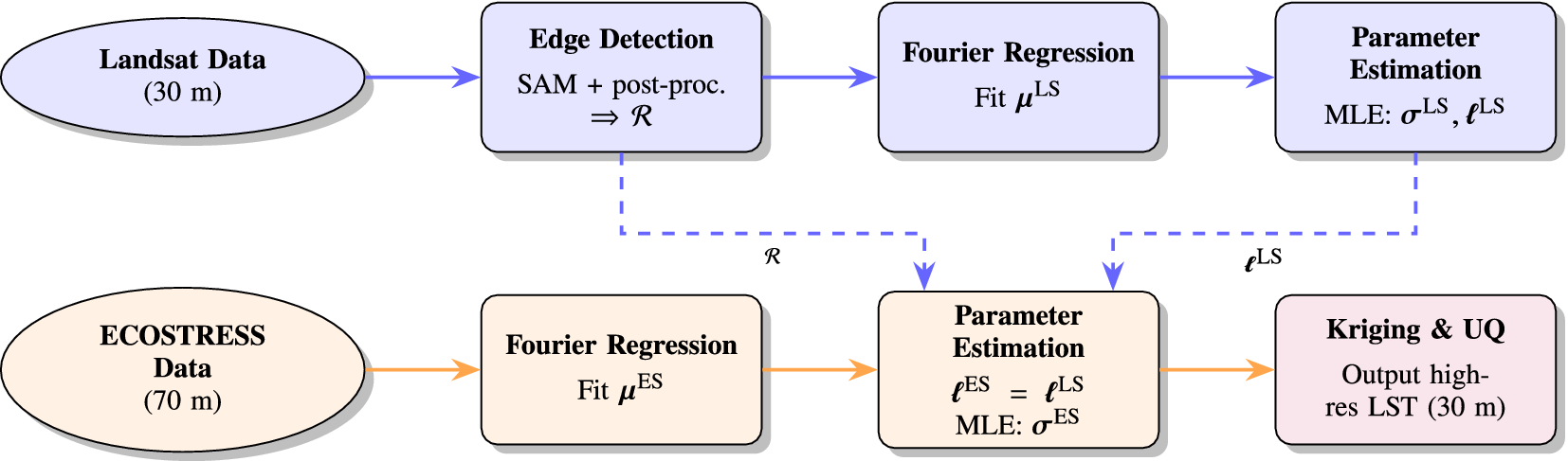
An overview of our downscaling pipeline is depicted in Figure 2.
Overview of the proposed downscaling pipeline. The Landsat data are shown in blue, the ECOSTRESS data are shown in orange, and the output of the algorithm is shown in purple.

Figure 2. Long description
The flowchart consists of two horizontal rows of nodes.
The top row (blue) begins with an oval labeled Landsat Data (30 m). A solid blue arrow points to a rectangular box labeled Edge Detection (S A M plus post-proc. yields R). From here, a solid blue arrow points to Fourier Regression (Fit mu super L S), which then points to Parameter Estimation (M L E: sigma super L S, l super L S).
The bottom row (orange) begins with an oval labeled ECOSTRESS Data (70 m). A solid orange arrow points to a rectangular box labeled Fourier Regression (Fit mu super E S). A solid orange arrow continues to Parameter Estimation (l super E S equals l super L S, M L E: sigma super E S).
Vertical interactions are shown with dashed lines:
- A dashed blue line carries R from the top Edge Detection box down to the bottom Parameter Estimation box.
- A dashed blue line carries l super L S from the top Parameter Estimation box down to the bottom Parameter Estimation box.
The final step in the bottom row is a purple rectangular box labeled Kriging and U Q (Output high-res L S T (30 m)), which receives a solid orange arrow from the bottom Parameter Estimation box.
2.1. Edge detection
First, we average six separate high-resolution Landsat images and use edge detection methods on the averaged image to identify boundaries between different agricultural fields. In our case, we use Meta’s Segment Anything Model (SAM), which is a state-of-the-art vision transformer (ViT) based segmentation model providing an over-segmentation of the input image—the model may produce partially or fully overlapping segments (Kirillov et al., Reference Kirillov, Mintun, Ravi, Mao, Rolland, Gustafson, Xiao, Whitehead, Berg, Lo, Dollár and Girshick2023). We experimented with several other methods, including the Canny, Sobel, and Laplace edge detection algorithms, but we found the SAM to work best in practice. Next, we post-process the over-segmented image to merge overlapping regions together using an algorithm described in Supplementary Appendix E. This post-processing step ensures that the final set of segments contains no overlaps. At this point, we have an estimated partition
$ \mathcal{R} $
 of the spatial domain into agricultural fields.
2.2. Fourier regression
Next, we fit
$ {\boldsymbol{\mu}}^{\mathrm{LS}} $
 separately for each pixel
$ x=\left(i,j\right) $
 using a Fourier regression with annual frequency:

where
$ t $
 is in units of days. We use ordinary least squares to fit the coefficients. We only use an annual frequency here because the Landsat satellite has a sun-synchronous orbit, meaning that the satellite orbits over the same spot on Earth at the same time of day every 16 days. As a result, we are unable to model the diurnal frequency for these data. Next, we fit the blurred mean
$ {\boldsymbol{\mu}}^{\mathrm{ES}}\ast {\kappa}_{\mathrm{blur}} $
 separately for each pixel
$ \left(i,j\right) $
 using a Fourier regression with annual and diurnal frequencies:

where
$ t $
 is in units of days. Note that we are fitting the blurred mean function here since we only observe the blurred data from ECOSTRESS. At last, we subtract the fitted mean functions from the observed data, so that we may model the residual data by zero-mean GPs. We see in Figure 1 (Supplementary Appendix C) that a single Fourier term is sufficient to capture the annual and diurnal cycles in the data, so that we can model the residuals by a mean-zero BDGP. Similarly, we depict the annual cycle fit for a random pixel in the Landsat data in Figure 2 (Supplementary Appendix C). The fitted cycles roughly capture the seasonal variations in land surface temperature, justifying our use of Fourier regression to model the mean function.
2.3. Parameter estimation
Since the uncertainties listed for the ECOSTRESS observations are all on the order of 0.1 degrees Kelvin, it is reasonable to choose
$ {\sigma}_{\mathrm{sensor}}=0.1 $
 . From Holmes et al. (Reference Holmes, Poulter, McCorkel, Jennings, Wu, Efremova, Shiklomanov, Johnson, Jhabvala and Hook2024), we know that the point spread function of ECOSTRESS approximately has a full-width at half-maximum (FWHM) of 160 m in each direction, which is roughly twice the nominal pixel size of 70 m. From the FWHM, we can calculate the standard deviation by
$ {\sigma}_{\mathrm{blur}}=\left(160/70\right)/\left(2\sqrt{2\ln (2)}\right)\approx 0.97 $
 in units of ECOSTRESS pixels. This computation is justified in Supplementary Appendix B.
Fixing
$ \mathcal{R} $
 , we now fit the remaining parameters of the BDGP model to the Landsat data. Note that each region can be fit independently here, which allows for easy parallelization and scalability to larger data. We do not include a temporal component in the covariance structure here, and instead sample far apart in time to reduce temporal correlation. As a result, we can treat these points as independent across time. We chose four sample dates
$ {t}_1,{t}_2,{t}_3,{t}_4 $
 that are ~3 months apart from each other. We write the likelihood of the observed data in the region
$ {R}_r $
 assuming that the observations are independent across time:

where
$ {K}_{R_r} $
 is the covariance matrix of the BDGP restricted to the region
$ r $
 and
$ {y}_{R_r,{t}_i}^{\mathrm{LS}} $
 is the observed residuals in the region
$ {R}_r $
 at time
$ {t}_i $
 . We estimate the parameters by maximizing this likelihood using the BFGS optimizer, adding a small nugget of
$ {10}^{-8}I $
 to the covariance matrix for numerical stability.
Next, we fix
$ \mathcal{R} $
 and assume that
$ {\mathbf{\ell}}^{\mathrm{ES}}={\mathbf{\ell}}^{\mathrm{LS}} $
 . Although the Landsat and ECOSTRESS data measure different quantities, it is reasonable to think that the length scale of the residual field should be similar across both datasets since they are over the same geographical region with similar spatial variation. This assumption is required to ensure identifiability of the parameters in our model, due to ill-posedness caused by the change of support present in the ECOSTRESS data. Then, we fit
$ {\boldsymbol{\sigma}}^{\mathrm{ES}} $
 to the ECOSTRESS data by maximum likelihood estimation.
We now ignore the existence of blurring from other regions at the edges of each region, and fit each region independently; this is justified due to the small relative scale of the blur kernel compared to the regions. Under this simplifying assumption, a consistent estimator given a single observation is

Here, we use
$ \mathrm{Var}\left({y}_{R_r}^{\mathrm{ES}}\right) $
 to denote the sample variance of the observed residuals in the region
$ {R}_r $
 , and we justify our use of this estimator in Supplementary Appendix A. We then aggregate our
$ {\sigma}_r^{\mathrm{ES}} $
 estimates from each separate time point by taking the median across times.
2.4. Kriging and uncertainty quantification
Finally, we use the fitted BDGP model for ECOSTRESS to do kriging (on a 30 m grid) and obtain high-resolution predictions of the residual LST field. Although the regions are no longer independent after blurring, we may treat each region independently after considering a
$ 4{\sigma}_{\mathrm{blur}} $
 -pixel neighborhood
$ {R}_r^{\prime } $
 around each region
$ {R}_r $
 . First, enumerate the pixels as
$ {x}_1,\dots, {x}_P $
 and define
$ {k}_{\ast } $
 as the covariance vector between
$ f\left({x}_{\ast}\right) $
 and all blurry observations in
$ {R}_r^{\prime } $
 :

Next, let
$ {K}_{R_r^{\prime }} $
 be the covariance matrix of the BDGP restricted to the region
$ {R}_r^{\prime } $
 :

Finally, let
$ {y}_{R_r^{\prime}}^{\mathrm{ES}} $
 be the observed residuals in region
$ {R}_r^{\prime } $
 ; namely,
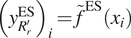
$ {\left({y}_{R_r^{\prime}}^{\mathrm{ES}}\right)}_i={\tilde{f}}^{\mathrm{ES}}\left({x}_i\right) $
 for
$ {x}_i\in {R}_r^{\prime } $
 . Using this notation, the kriging formula (Cressie, Reference Cressie1991) gives us the conditional mean in the region
$ {R}_r $
 at location
$ {x}_{\ast } $
 as

Repeating this computation for each region
$ {R}_r $
 gives us the full kriging prediction
$ {\hat{f}}^{\mathrm{ES}} $
 . By reconstructing each region separately, we can parallelize this step and maintain computational tractability as long as each region is not too large. In this work, we do not reconstruct the road region, since it is too large to reconstruct efficiently using our current implementation. Although the roads can be reconstructed by splitting into several overlapping subregions, the roads are not of primary interest in agricultural applications, so we leave this for future work. Additionally, because we still estimate the parameters for the road region, this does not affect the reconstructions in other regions.
Next, to compute the variance of the kriging prediction at the location
$ {x}_{\ast } $
 in region
$ {R}_r $
 , we use the formula

For instance, this formula can be found in Cressie (Reference Cressie1991). Note that the resulting reconstruction is only of the residual field; to obtain the full LST field, we would need to add back a deconvolved mean function, which can be done more carefully using methods from spatial statistics. However, we leave this for future work.
3. Results
For our analysis, we consider an agricultural region of 6
$ {\mathrm{km}}^2 $
 near the Salton Sea in southern California (USA). We use data from the SR_B5 channel of the Landsat 8 satellite (Roy et al., Reference Roy, Wulder, Loveland, C.E, Allen, Anderson, Helder, Irons, Johnson, Kennedy, Scambos, Schaaf, Schott, Sheng, Vermote, Belward, Bindschadler, Cohen, Gao, Hipple, Hostert, Huntington, Justice, Kilic, Kovalskyy, Lee, Lymburner, Masek, McCorkel, Shuai, Trezza, Vogelmann, Wynne and Zhu2014), which measures surface reflectance in the near-infrared spectrum of light. Our goal is to deconvolve an ECOSTRESS (Fisher et al., Reference Fisher, Lee, Purdy, Halverson, Dohlen, Cawse-Nicholson, Wang, Anderson, Aragon, Arain, Baldocchi, Baker, Barral, Bernacchi, Bernhofer, Biraud, Bohrer, Brunsell, Cappelaere, Castro-Contreras, Chun, Conrad, Cremonese, Demarty, Desai, De Ligne, Foltýnová, Goulden, Griffis, Grünwald, Johnson, Kang, Kelbe, Kowalska, Lim, Maïnassara, McCabe, Missik, Mohanty, Moore, Morillas, Morrison, Munger, Posse, Richardson, Russell, Ryu, Sanchez-Azofeifa, Schmidt, Schwartz, Sharp, Šigut, Tang, Hulley, Anderson, Hain, French, Wood and Hook2020) LST image taken in January 2021 using the Landsat data as a proxy for modeling the agricultural field structure. All code to run our experiments is provided in Dandapanthula (Reference Dandapanthula2026). We preprocess both datasets to be on a common grid with 30 m resolution. For all of our analysis, we manually choose images that are relatively cloud-free in our region of interest, and do not account for missingness. All of our parameter estimation and kriging procedures work with slight modifications to the code in the presence of some missing data. Similarly, large amounts of missingness can be handled by including a temporal component in the Gaussian process, but this is left for future work.
We target an ECOSTRESS LST image taken in January 2021. The Landsat and ECOSTRESS mean functions are each fit using all available images of the region. The ECOSTRESS covariance parameter
$ {\boldsymbol{\sigma}}^{\mathrm{ES}} $
 and the Landsat covariance parameters
$ \left({\boldsymbol{\sigma}}^{\mathrm{LS}},{\mathbf{\ell}}^{\mathrm{LS}}\right) $
 are each fit from four images, ~3 months apart, all taken before the target image to ensure that our fitted parameters generalize. Edge detection is performed on an average of six separate Landsat images, none of which coincides with the target date.
We begin by showing the results of the edge detection method on the average of 6 Landsat images (starting in November 2021 and spread out by ~2 months) in our region of interest in Figure 3. Hence, we confirm that the final regions capture the agricultural field structure relatively well, and there are no overlaps between different regions after post-processing.
Side-by-side comparison of (a) the averaged Landsat image, (b) the over-segmented image from SAM, and (c) the final regions after post-processing.

Figure 3. Long description
The figure consists of three horizontal panels showing the same grid-like agricultural landscape.
* Panel a, labeled Averaged Landsat image, displays a heat map of rectangular fields. The color gradient ranges from deep blue to vibrant orange and red, indicating varying spectral intensities across the grid. A prominent vertical linear feature, likely a road or canal, bisects the right third of the frame from North to South.
* Panel b, labeled S A M oversegmentation, shows the same area processed by the Segment Anything Model. The fields are now represented as solid, multi-colored polygons. The segmentation is highly granular, with many individual fields broken into smaller sub-sections of different colors like pink, green, yellow, and grey. The background between segments is a uniform dark blue.
* Panel c, labeled Regions after post-processing, shows the refined output. The segments are larger and more cohesive than in panel b, with black outlines defining the boundaries of each agricultural plot. The colors are more muted and transparent, overlaid on the original grayscale texture of the fields. The small, fragmented segments from the previous step have been merged into distinct, clean rectangular and polygonal regions that align with the physical boundaries seen in the original Landsat data.
Next, we show our original ECOSTRESS image from January 2021 in Figure 4a (which we would like to deblur), along with the resulting residuals after subtracting the fitted mean function in Figure 4b. As expected, the residuals contain significant spatial structure that we can model using our BDGP approach. This day was particularly cold, leading to negative residuals across most of the image. To verify that our mean function is sensible for the Landsat data, we also show the residuals for a sample Landsat image in Figure 4d. Again, we see that the residuals contain significant spatial structure that we can model using our BDGP approach, and are close to zero.
Side-by-side comparison of (a) the original ECOSTRESS image, (b) the ECOSTRESS residuals after subtracting the fitted mean function, (c) the original Landsat image, and (d) the Landsat residuals after subtracting the fitted mean function.

Figure 4. Long description
The multi-panel figure consists of four square heat maps arranged in a single row.
* Panel a, ECOSTRESS original: A pixelated heat map showing Land Surface Temperature L S T in Kelvin K. The color scale ranges from dark purple 293 K to bright yellow 299 K. High-temperature yellow clusters are concentrated on the left and center-right.
* Panel b, ECOSTRESS residuals: Shows the data after subtracting the mean function. The color scale ranges from blue negative 4 K to red positive 4 K. Most of the area is light blue, with distinct orange-red clusters indicating positive residuals where the original image had high temperatures.
* Panel c, Landsat original: A high-resolution grid-like map of Surface Reflectance S R B 5. The color scale ranges from dark purple 0.25 to bright yellow 0.60. The map shows sharp rectangular agricultural fields, with a few fields appearing bright yellow against a dark green and blue background.
* Panel d, Landsat residuals: Shows the Landsat data after mean subtraction. The color scale ranges from blue negative 0.10 to red positive 0.10. The rectangular field boundaries are highly visible, with specific fields showing strong positive red residuals or strong negative dark blue residuals compared to the surrounding light blue areas.
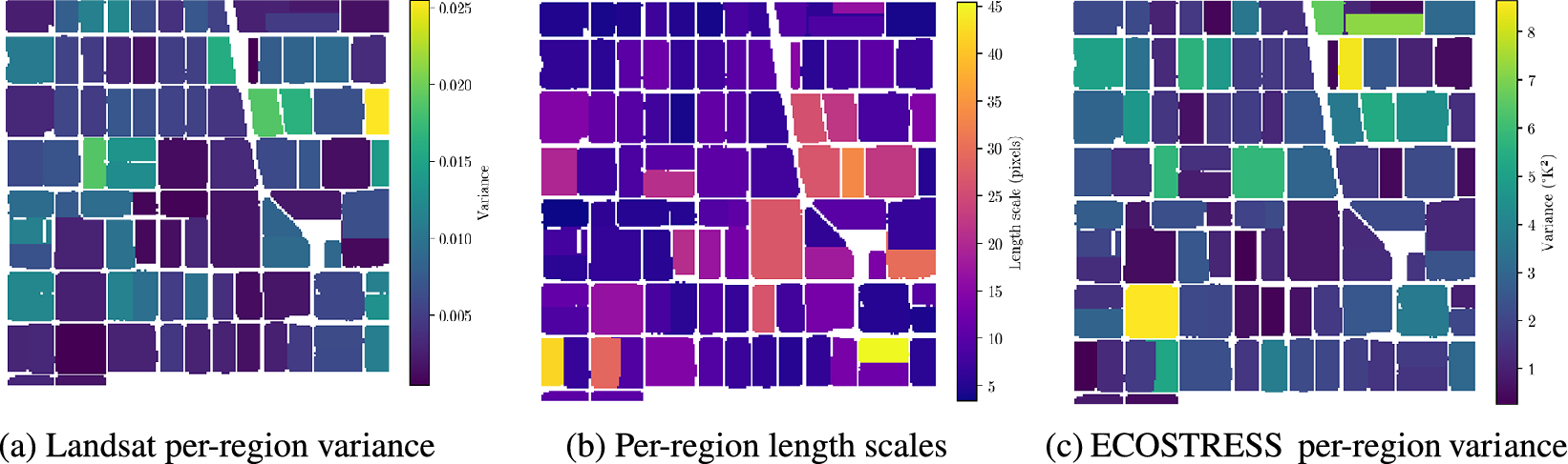
Next, we show the fitted parameters for each region in Figure 5. We see that the length scales vary significantly across regions, justifying our use of a block-diagonal GP to model the agricultural field structure. Furthermore, the optimization procedure appears to have found reasonable parameter values for both datasets. Finally, we depict the kriging results along with the resulting uncertainty quantification in Figure 6. The kriging predictions effectively deblur many of the features present in the original ECOSTRESS image, and we can quantify the uncertainty in our predictions through the per-pixel variance. Note that the uncertainty for each region is higher near the edges; this is because the statistical assumption of independence between regions increases the uncertainty of the reconstruction near the edges.
Fitted parameters for each region: (a) Landsat per-region variance, (b) per-region length scales (shared between Landsat and ECOSTRESS), and (c) ECOSTRESS per-region variance.

Figure 5. Long description
A three-panel set of geographical heat maps. Each map displays a grid of rectangular agricultural plots separated by white boundaries.
Panel a, labeled Landsat per-region variance, shows values ranging from 0.005 to 0.025 on a vertical color bar. The distribution is mostly dark purple (low variance) with scattered teal and yellow plots (high variance) in the Northeast and East-central areas.
Panel b, labeled Per-region length scales, uses a scale from 5 to 45 pixels. This map shows higher values (yellow and orange) concentrated in the South-central and Southeast regions, while the Northwest is dominated by dark purple and indigo (low length scales).
Panel c, labeled ECOSTRESS per-region variance, uses a scale from 1 to 8 K super 2. The map shows a high-variance yellow plot in the Southwest and another in the North, while the majority of the central and Eastern plots remain in the low-variance dark blue range.
All three maps share a distinct diagonal white feature cutting from the North-central edge toward the Southeast.
Comparison of (a) the original ECOSTRESS residual image, (b) the kriging mean prediction, and (c) two per-pixel standard deviations for the kriging predictions.

Figure 6. Long description
A three-panel set of heat maps showing spatial temperature data.
Panel a, labeled Original E C O S T R E S S residual, shows a continuous, blurry heat map with blue representing negative values and orange-red representing positive values. A vertical color bar on the right is labeled Residual degrees K, ranging from minus 4 to plus 4.
Panel b, labeled Kriging mean prediction, shows the same spatial area but masked into a grid of rectangular agricultural plots separated by white lines. The color distribution matches panel a, with a vertical color bar labeled Prediction degrees K, ranging from minus 4 to plus 4.
Panel c, labeled Kriging per-pixel 2 sigma, shows the uncertainty of the predictions within the same rectangular grid. The color scale uses a dark purple to yellow gradient. A vertical color bar on the right is labeled Uncertainty degrees K, ranging from 0.0 at the bottom to 0.8 at the top. Darker purple areas indicate lower uncertainty, while yellow-orange borders and specific plots indicate higher uncertainty reaching 0.8 sigma.
We verify that our method works well by manually blurring and recovering a high-resolution Landsat image in Supplementary Appendix D.
4. Discussion
In this work, we proposed a novel statistical method for downscaling LST data from the ECOSTRESS mission using high-resolution data from the Landsat mission as a proxy for modeling agricultural field structure. By leveraging a block-diagonal Gaussian process model, we were able to capture the spatial structure of agricultural fields and perform scalable inference. Our results demonstrate that the proposed method effectively deblurs ECOSTRESS LST data, producing higher-resolution estimates along with uncertainty quantification. The fitted parameters varied significantly across regions, justifying our use of a block-diagonal GP to model the agricultural field structure. Furthermore, our toy example verified that the method can successfully reconstruct blurred images, recovering features present in the original data.
Despite the strengths of our proposed framework, several limitations remain. First, while we estimate parameters for the network of roads between agricultural fields, we do not reconstruct this region in the current work due to its size. Second, despite the strong performance of the segmentation method using the Segment Anything Model (SAM), future studies might benefit from incorporating alternative segmentation algorithms or incorporating the uncertainty of the segmentation. Furthermore, the performance of our method is inherently limited by the quality of the ECOSTRESS data, which suffers from blur and artifacts resulting from physical damage to the sensor. This extends to our assumptions that the blur kernel and additive sensor noise are Gaussian; these assumptions may be inexact, given that Holmes et al. (Reference Holmes, Poulter, McCorkel, Jennings, Wu, Efremova, Shiklomanov, Johnson, Jhabvala and Hook2024) demonstrate that the ECOSTRESS point spread function is not perfectly Gaussian. Finally, to ensure identifiability, we rely on the simplifying assumption that the length scale parameters for ECOSTRESS and Landsat are identical, a condition that may not strictly hold in practice.
In future work, the Block-Diagonal Gaussian Process (BDGP) kernel could be augmented with a temporal length scale to capture time-varying dynamics. This would allow for gap-filling in time, which is of great practical value, given the large amount of missingness. Additionally, replacing the standard squared exponential kernel with a sharper Matérn kernel could more accurately model the roughness of the field. From a computational perspective, further optimizing the code would allow scalability to larger datasets. Another future direction is to model the mean of the high-resolution land surface temperature field, possibly using an auxiliary higher-resolution data source. Finally, the roads could be partitioned into smaller, more tractable regions so that they may be reconstructed as well.
The broader implication of this work is that by modeling a field structure using a block-diagonal GP, we obtain a pipeline for building a scalable statistical model for data fusion of sensors with complementary strengths. This approach accounts for both the change of support and field structure present in the data, allowing us to perform scalable statistical modeling on large datasets. For instance, this method could be applied to urban heat island modeling, European agricultural landscapes (with more irregular field shapes), or other remote sensing contexts where high-resolution proxies are available.
Supplementary material
The supplementary material for this article can be found at http://doi.org/10.1017/eds.2026.10052.
Acknowledgments
This research was partially carried out at the Jet Propulsion Laboratory, California Institute of Technology, under a contract with the National Aeronautics and Space Administration (80NM0018D0004).
Author contribution
Conceptualization: S.D., M.J., and M.K.; Methodology: S.D. and M.K.; Data visualization: S.D.; Software: S.D.; Resources: M.J., G.H., M.P.-C., and M.K.; Supervision: M.J., M.P.-C., G.H., and M.K.; Writing—original draft: S.D.; Writing—review and editing: M.J. and M.K. All authors approved the final submitted draft.
Competing interests
The authors declare none.
Data availability statement
Code can be found at https://github.com/sanjitdp/downscaling-lst. Replication data can be obtained from https://appeears.earthdatacloud.nasa.gov/ using the .json request files contained in the code repository.
Ethics statement
The research meets all ethical guidelines, including adherence to the legal requirements of the study country.
Funding statement
SD was sponsored by the CMU Department of Statistics and Data Science to attend Climate Informatics 2026.
Provenance statement
This article is part of the Climate Informatics 2026 proceedings and was accepted in Environmental Data Science based on the Climate Informatics peer review process.





 Open access

