2.1 Sensitivity testing and scenario weights

The purpose of SWIM is to enable sensitivity analysis of models implemented in a Monte Carlo simulation framework, by distorting (stressing) some of the models’ components and monitoring the resulting impact on quantities of interest. To clarify this idea and explain how SWIM works, we first define the terms used. 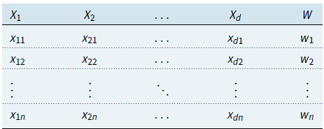By a model, we mean a set of n (typically simulated) realisations from a vector of random variables $(X_1,\dots,X_d)$ , along with scenario weights W assigned to individual realisations, as shown in Table 1. Hence, each of the columns 1 to d corresponds to a random variable, called a model component, while each row corresponds to a scenario, that is, a state of the world.

Table 1.

Illustration of the SWIM framework, that is the baseline model, the stressed model, and the scenario weights.

There is a conceptual distinction between the model from which the scenarios are simulated and the model as understood here. Specifically, as we are considering the case when an analyst has access to simulated scenarios only, and not the data-generating mechanism, we are consistently working with the empirical probability measure and any expectations or probabilities stated below are given with respect to that measure. Furthermore, as we work on an empirical space, we systematically conflate a random variable with its vector of realisations – in particular, the scenario weights W can be identified with a Radon–Nikodym derivative on that space. For relevant notation on the space we are working on, see section 3.

Each scenario has a scenario weight, shown in the last column, such that, scenario i has probability $\frac{w_i}{n}$ of occurring. Scenario weights are always greater or equal than 0 and have an average of 1. When all scenario weights are equal to 1, such that the probability of each scenario is $\frac 1 n$ (the standard Monte Carlo framework), we call the model a baseline model – consequently, weights of a baseline model will never be explicitly mentioned. When scenario weights are not identically equal to 1, such that some scenarios are more weighted than others, we say that we have a stressed model.

The scenario weights make the joint distribution of model components under the stressed model different, compared to the baseline model. For example, under the baseline model, the expected value of $X_1$ and the cumulative distribution function of $X_1$ , at threshold t, are respectively given by:

\begin{equation*}E(X_1)=\frac 1 n \sum_{i=1}^nx_{1i},\quad F_{X_1}(t)= P(X_1\leq t)=\frac 1 n \sum_{i=1}^n \mathbf 1 _{x_{1i}\leq t}\end{equation*}

where $\mathbf 1 _{x_{1i}\leq t}=1$ if $x_{1i}\leq t$ and 0 otherwise. For a stressed model with scenario weights W, the expected value $E^W$ and cumulative distribution function $F^W$ become

\begin{equation*}E^W(X_1)=\frac 1 n \sum_{i=1}^n w_i x_{1i},\quad F_{X_1}^W(t)=P^W(X_1\leq t)=\frac 1 n \sum_{i=1}^n w_i \mathbf 1 _{x_{1i}\leq t}\end{equation*}

Similar expressions can be derived for more involved quantities, such as higher (joint) moments and quantiles.

The logic of stressing a model with SWIM then proceeds as follows. An analyst or modeller is supplied with a baseline model, in the form of a matrix of equiprobable simulated scenarios of model components. The modeller wants to investigate the impact of a change in the distribution of, say, $X_1$ . To this effect, she chooses a stress on the distribution of $X_1$ , for example, requiring that $E^W(X_1)=m$ ; we then say that she is stressing $X_1$ and, by extension, the model. Subsequently, SWIM calculates the scenario weights such that the stress is fulfilled and the distortion to the baseline model induced by the stress is as small as possible; specifically, the Kullback–Leibler divergence (or relative entropy) between the baseline and stressed models is minimised. (See section 3.1 for more detail on the different types of possible stresses and the corresponding optimisation problems). Once scenario weights are obtained, they can be used to determine the stressed distribution of any model component or function of model components. For example, for scenario weights W obtained through a stress on $X_1$ , we may calculate

\begin{equation*}E^W(X_2)=\frac 1 n\sum_{i=1}^n w_i x_{2i},\quad E^W(X_1^2+X_2^2)=\frac 1 n \sum_{i=1}^n w_i \left(x_{1i}^2+ x_{2i}^2 \right)\end{equation*}

Through this process, the modeller can monitor the impact of the stress on $X_1$ on any other random variable of interest. It is notable that this approach does not necessitate generating new simulations from a stochastic model. As the SWIM approach requires a single set of simulated scenarios (the baseline model), it offers a clear computational benefit.

2.2 An introductory example

Here, through an example, we illustrate the basic concepts and usage of SWIM for sensitivity analysis. More advanced usage of SWIM and options for constructing stresses are demonstrated in sections 3 and 4.

In sensitivity analysis, one often considers a model with a vector of inputs $\mathbf Z$ and an output $Y=g(Z)$ , for some aggregation function g that maps inputs to the real line. Then, the importance of model inputs can be investigated by stressing the distribution of inputs and observing the impact on the output distribution and vice versa (Pesenti et al., Reference Pesenti, Millossovich and Tsanakas2019). (We note that in SWIM there is no ex ante assumption about which of the model components $(X_1, \dots,X_d)$ should be interpreted as inputs or outputs – these variables could represent any randomly varying quantity in the model. For that reason, we use $X_i$ for variable labels when documenting the SWIM’s capabilities, but use alternative notation in illustrations where variables have specific interpretable meanings, as in the current section and in the case study of section 4).

Here, we consider a simple portfolio model, with the portfolio loss defined by $Y=Z_1+Z_2+Z_3$ . The random variables $Z_1,Z_2,Z_3$ represent normally distributed losses, with $Z_1\sim N(100,40^2)$ , $Z_2\sim Z_3\sim N(100,20^2)$ . $Z_1$ and $Z_2$ are correlated, while $Z_3$ is independent of $(Z_1,Z_2)$ . Our purpose in this example is to investigate how a stress on the loss $Z_1$ impacts on the overall portfolio loss Y. First, we derive simulated data from the random vector $(Z_1,Z_2,Z_3,Y)$ , forming our baseline model.

Now, we introduce a stress to our baseline model. For our first stress, we require that the mean of $Z_1$ is increased from 100 to 110. This is done using the stress function, which generates as output a SWIM object, which we call str.mean. This object stores the stressed model, that is, the realisations of the model components and the scenario weights. In the function call, the argument k = 1 indicates that the stress is applied on the first column of dat, that is, on the realisations of the random variable $Z_1$ .

The summary function, applied to the SWIM object str.mean, shows how the distributional characteristics of all random variables change from the baseline to the stressed model. In particular, we see that the mean of $Z_1$ changes to its required value, while the mean of Y also increases. Furthermore, there is a small impact on $Z_2$ , due to its positive correlation to $Z_1$ .

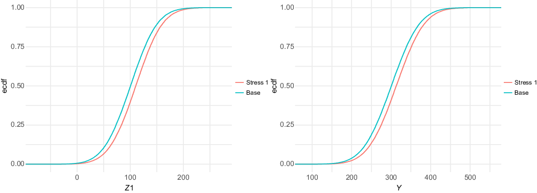
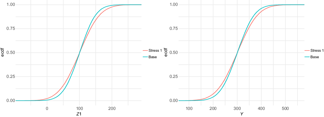
Beyond considering the standard statistics evaluated via the summary function, stressed probability distributions can be plotted. In Figure 1, we show the impact of the stress on the cumulative distribution functions (cdf) of $Z_1$ and Y. It is seen how the stressed cdfs are lower than the original (baseline) ones. Loosely speaking, this demonstrates that the stress has increased (in a stochastic sense) both random variables $Z_1$ and Y. While the stress was on $Z_1$ , the impact on the distribution of the portfolio Y is clearly visible.

Figure 1

Baseline and stressed empirical distribution functions of model components $Z_1$ (left) and Y (right), subject to a stress on the mean of $Z_1$ .

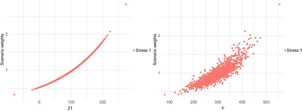
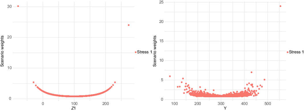
The scenario weights, given their central role, can be extracted from a SWIM object. In Figure 2, the scenario weights from str.mean are plotted against realisations from $Z_1$ and Y, respectively. It is seen how the weights are increasing in the realisations from $Z_1$ . This is a consequence of the weights’ derivation via a stress on the model component $Z_1$ . The increasingness shows that those scenarios for which $Z_1$ is largest are assigned a higher weight. The relation between scenario weights and Y is still increasing (reflecting that high outcomes of Y tend to receive higher weights), but no longer deterministic (showing that Y is not completely driven by changes in $Z_1$ ). 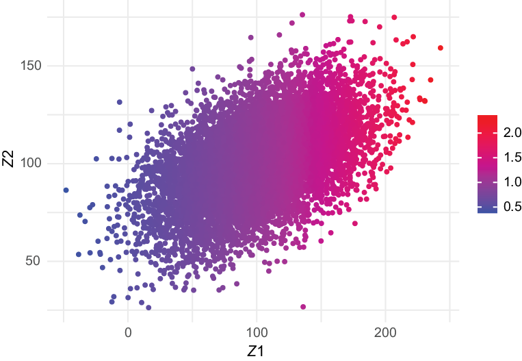Figure 3 displays the scenario weights as a function of the input variable $Z_1$ and $Z_2$ . The different colours of the scenario weights indicate their relative sizes. We observe that the scenario weights are increasing jointly in $Z_1$ and $Z_2$ .

Figure 2

Scenario weights against observations of model components $Z_1$ (left) and Y (right), subject to a stress on the mean of $Z_1$ .

Figure 3

Scenario weights for observations of model components $Z_1$ , $Z_2$ subject to a stress on the mean of $Z_1$ .

The stress to the mean of $Z_1$ did not impact the volatility of either $Z_1$ or Y, as can be seen by the practically unchanged standard deviations in the output of summary(str.mean). Thus, we introduce an alternative stress that keeps the mean of $Z_1$ fixed at 100, but increases its standard deviation from 40 to 50. This new stress is seen to impact the standard deviation of the portfolio loss Y.

Furthermore, in Figure 4, we compare the baseline and stressed cdfs of $Z_1$ and Y, under the new stress on $Z_1$ . The crossing of probability distributions reflects the increase in volatility.

Figure 4

Baseline and stressed empirical distribution functions of model components $Z_1$ (left) and Y (right), subject to a stress on the standard deviation of $Z_1$ .

The different way in which a stress on the standard deviation of $Z_1$ impacts on the model, compared to a stress on the mean, is reflected by the scenario weights. Figure 5 shows the pattern of the scenario weights and how, when stressing standard deviations, higher weight is placed on scenarios where $Z_1$ is extreme, either much lower or much higher than its mean of 100.

Figure 5

Scenario weights against observations of model components $Z_1$ (left) and Y (right), subject to a stress on the standard deviation of $Z_1$ .

Finally, we ought to note that not all stresses that one may wish to apply are feasible. Assume for example that we want to increase the mean of $Z_1$ from 100 to 300, which exceeds the maximum realisation of $Z_1$ in the baseline model. Then, clearly, no set of scenario weights can be found that produce a stress that yields the required mean for $Z_1$ ; consequently, an error message is produced.

## Error in stress_moment(x = x, f = means, k = as.list(k), m = new_means,:

Values in m must be in the range of f(x)

## [1] 273

3.1 Stressing a model

We briefly introduce key concepts, using slightly more technical language compared to section 2. A model consists of a random vector of model components $\mathbf X = (X_1,\dots,X_d)$ and a probability measure; we denote the probability measure of a baseline model by P and that of a stressed model by $P^W$ , where $W= \frac{dP^W}{dP}$ , satisfying $E(W)=1$ and $W\geq 0$ , is a Radon–Nikodym derivative. In a Monte Carlo simulation context, the probability space is discrete with n states $\Omega=\{\omega_1,\dots,\omega_n\}$ , each of which corresponds to a simulated scenario. To reconcile this formulation with the notation of section 2, we denote, for $i=1, \dots, n,\ j=1,\dots, d$ , the realisations $${X_j}({\omega _i}): = {x_{ji}}$$ and $$W({\omega _i}): = {w_i}$$ ; the latter are the scenario weights. Under the baseline model, each scenario has the same probability $P(\omega_i)=1/n$ , while under a stressed model it is $P^W(\omega_i)=W(\omega_i)/n=w_i/n$ .

The stressed model thus arises from a change of measure from P to $P^W$ , which entails the application of scenario weights $w_1,\dots, w_n$ on individual simulations. SWIM calculates scenario weights such that model components fulfil specific stresses, while the distortion to the baseline model is as small as possible when measured by the Kullback–Leibler divergence (or relative entropy). The Kullback–Leibler divergence of the probability measure of the baseline model P with respect to that of a stressed model $P^W$ is defined as:

(1) \begin{equation}E(W \log (W)) = \int \frac{dP^W}{dP} \log \left( \frac{dP^W}{dP}\right)\, dP\end{equation}

The Kullback–Leibler divergence is non-negative, vanishes if and only if the probabilities coincide, that is, if $P = P^W$ , and is often used as a measure of discrepancy between probability measures (Pesenti et al., Reference Pesenti, Millossovich and Tsanakas2019).

A stressed model is defined as the solution to

(2) \begin{equation}\min_{ W } E(W \log (W)), \quad\text{subject to constraints on } \mathbf X \text{ under } P^W\end{equation}

In what follows, we denote by a superscript W operators under the stressed model, such as $F^W, E^W$ for the probability distribution and expectation under the stressed model, respectively. We refer to Pesenti et al. (Reference Pesenti, Millossovich and Tsanakas2019) and references therein for further mathematical details and derivations of solutions to (2).

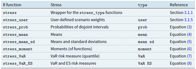
Table 2 provides a collection of all implemented types of stresses in the SWIM package. The precise constraints of (2) are explained below.

The solutions to the optimisations (3) and (7) are worked out fully analytically (Pesenti et al., Reference Pesenti, Millossovich and Tsanakas2019), whereas problems (4), (5), (6), and (8) require some root-finding. Specifically, problems (4), (5), and (6) rely on the package nleqslv, whereas (8) uses the uniroot function.

3.1.1 The stress function and the SWIM object

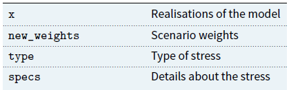
The stress function is a wrapper for the stress_type functions, where stress(type = “type”,) and stress_type are equivalent. The stress function solves optimisation (2) for constraints specified through type and returns a SWIM object, that is, a list including the elements shown in Table 3:

Table 2.

Implemented types of stresses in SWIM.

Table 3.

The SWIM object, returned by any stress function.

The data frame containing the realisations of the baseline model, x in the above table, can be extracted from a SWIM object using get_data. Similarly, get_weights and get_weightsfun provide the scenario weights, respectively, the functions that, when applied to x, generate the scenario weights. The details of the applied stress can be obtained using get_specs.

3.1.2 Stressing disjoint probability intervals

Stressing probabilities of disjoint intervals allows defining stresses by altering the probabilities of events pertaining to a model component. The scenario weights are calculated via stress_prob, or equivalently stress(type = “prob”,), and the disjoint intervals are specified through the lower and upper arguments, the endpoints of the intervals. Specifically,

stress_prob solves (2) with the constraints:

(3) \begin{equation}P^W(X_j \in B_k) = \alpha_k, k = 1, \ldots, K \end{equation}

for disjoint intervals $B_1, \ldots, B_K$ with $P(X_j \in B_k) >0$ for all $k = 1, \ldots, K$ , and $\alpha_1, \ldots, \alpha_K > 0$ such that $\alpha_1 + \ldots + \alpha_K \leq 1$ and a model component $X_j$ .

3.1.3 Stressing moments

The functions stress_mean, stress_mean_sd, stress_moment implement the solution in Csiszár (Reference Csiszár1975) and provide stressed models with moment constraints. The function stress_mean returns a stressed model that fulfils constraints on the first moment of model components. Specifically,

stress_mean solves (2) with the constraints:

(4) \begin{equation}E^W(X_j) = m_j, j \in J \end{equation}

for $m_j, j \in J$ , where J is a subset of $\{1, \ldots, d\}$ .

The arguments $m_j$ are specified in the stress_mean function through the argument new_means. The stress_mean_sd function allows to stress simultaneously the mean and the standard deviation of model components. Specifically,

stress_mean_sd solves (2) with the constraints:

(5) \begin{equation}E^W(X_j) = m_j \text{ and Var}^W(X_j) = s_j^2 , j \in J \end{equation}

for $m_j, s_j, j \in J$ , where J is a subset of $\{1, \ldots, d\}$ .

The arguments $m_j, s_j$ are defined in the stress_mean_sd function by the arguments new_means and new_sd, respectively. The functions stress_mean and stress_mean_sd are special cases of the general stress_moment function, which allows for stressed models with constraints on functions of the (joint) moments of model components. Specifically,

for $k = 1, \ldots, K$ , $J_k$ subsets of $\{1, \ldots, d\}$ and functions $f_k \colon \mathbb{R}^{|J_k|} \to \mathbb{R}$ , stress_moment solves (2) with the constraints:

(6) \begin{equation}E^W(\,f_k(\mathbf X_{J_k}) ) = m_k, k = 1, \ldots, K \end{equation}

for $m_k, k=1, \dots,K$ and $\mathbf X_{J_k}$ , the subvector of model components with indices in $J_k$ .

Note that stress_moment not only allows to define constraints on higher moments of model components but also to construct constraints that apply to multiple model components simultaneously. For example, the stress $E^W(X_h X_l) =m_k$ is achieved by setting $f_k(x_h, x_l) = x_h x_l$ in (6) above. The functions stress_mean, stress_mean_sd and stress_moment can be applied to multiple model components and are the only stress functions that have scenario weights calculated via numerical optimisation, using the nleqslv package. Thus, depending on the choice of constraints, existence or uniqueness of a stressed model is not guaranteed. The stress_moment function will print a message stating the specified values for the required moments, alongside the moments achieved under the stressed model resulting from the function call. If the two match, the stress specification has been successfully fulfilled.

3.1.4 Stressing risk measures

The functions stress_VaR and stress_VaR_ES provide stressed models, under which a model component fulfils a stress on the risk measures VaR and/or ES. The VaR at level $0 < \alpha < 1$ of a random variable Z with distribution F is defined as its left-inverse evaluated at $\alpha$ , that is

\begin{equation*}\text{VaR}_\alpha(Z) = F^{-1}(\alpha) = \inf\{ y \in \mathbb{R} | F(y) \geq \alpha\}\end{equation*}

The ES at level $0 < \alpha < 1$ of a random variable Z is given by:

\begin{equation*}\text{ES}_\alpha(Z) =\frac{1}{1-\alpha}\int_\alpha^1 \text{VaR}_u(Z) \textrm{d}u\end{equation*}

The details of the constraints that stress_VaR and stress_VaR_ES solve, are as follows:

For $0< \alpha <1$ and q, s such that $q < s$ , stress_VaR solves (2) with the constraint:

(7) \begin{equation}\text{VaR}_{\alpha }^W(X_j) = q \end{equation}

and stress_VaR_ES solves (2) with the constraints:

(8) \begin{equation}\text{VaR}_{\alpha }^W(X_j) = q \text{ and ES}_{\alpha }^W(X_j) = s\end{equation}

Note that, since SWIM works with discrete distributions, the exact required constraints may not be achievable, see Pesenti et al. (Reference Pesenti, Millossovich and Tsanakas2019) for more details. In that case, the stress function will print a message with the achieved and required constraints. For example, stress_VaR will return scenario weights inducing the largest quantile in the dataset smaller or equal to the required VaR (i.e. q); this guarantees that $P^W(X_j\leq q)=\alpha$ .

3.2 Analysis of stressed models

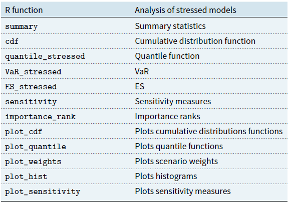
Table 4 provides a complete list of all implemented R functions in SWIM for analysing stressed models, which are described below in detail.

Table 4.

Implemented R function in SWIM for analysing stressed models.

3.2.1 Distributional comparison

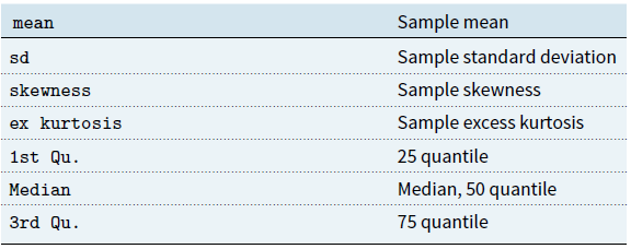
The SWIM package contains functions to compare the distribution of model components under different (stressed) models. The function summary is a method for an object of class SWIM and provides summary statistics of the baseline and stressed models. If the SWIM object contains more than one set of scenario weights, each corresponding to one stressed model, the summary function returns for each set of scenario weights a list, containing the elements shown in Table 5.

The empirical distribution function of model components under a stressed modelFootnote ¹ can be calculated using the cdf function of the SWIM package, applied to a SWIM object. To calculate sample quantiles of stressed model components, the function quantile_stressed can be used. The function VaR_stressed and ES_stressed provide the stressed VaR and ES of model components, which is of particular interest for stressed models resulting from constraints on risk measures, see section 3.1.4. (While quantile_stressed works very similarly to the base R function quantile, VaR_stressed provides better capabilities for comparing different models and model components.)

Implemented visualisation of distribution functions are plot_cdf, for plotting empirical distribution functions, plot_quantile, for plotting empirical quantile functions, and plot_hist, for plotting histograms of model components under different (stressed) models. The scenario weights can be plotted against a model component using the function plot_weights.

Table 5.

The output of the summary function applied to a SWIM object.

Table 6.

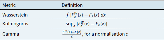
Definition of the sensitivity measures implemented in SWIM.

4.1 A credit risk portfolio

In this section, we provide a detailed case study of the use of SWIM in analysing a credit risk model. Through this analysis, we also illustrate more advanced capabilities of the package. The credit model in this section is a conditionally binomial loan portfolio model, including systematic and specific portfolio risk. We refer to the Appendix A for details about the model and the generation of the simulated data. A key variable of interest is the total aggregate portfolio loss $L = L_1 + L_2 + L_3$ , where $L_1, L_2, L_3$ are homogeneous subportfolios on a comparable scale (say, thousands of). The dataset contains 100,000 simulations of the portfolio L, the subportfolios $L_1, L_2, L_3$ as well as the random default probabilities within each subportfolio, $H_1, H_2, H_3$ . These default probabilities represent the systematic risk within each subportfolio, while their dependence structure represents a systematic risk effect between the subportfolios. We may thus think of L as the model output, $H_1,H_2,H_3$ as model inputs, and $L_1,L_2,L_3$ as intermediate model outputs.

The simulated data of the credit risk portfolio are included in the SWIM package and can be accessed via data(“credit_data”). A snippet of the dataset looks as follows:

4.2 Stressing the portfolio loss

In this section, we follow a reverse sensitivity approach, similar to Pesenti et al. (Reference Pesenti, Millossovich and Tsanakas2019). Specifically, we study the effects that stresses on (the tail of) the aggregate portfolio loss L have on the three subportfolios. This enables us to assess their comparative importance. If a subportfolio’s loss distribution substantially changes following a stress on the portfolio loss, we interpret this as a high sensitivity to that subportfolio.

First, we impose a 20% increase on the VaR at level 90% of the portfolio loss.

## Stressed VaR specified was 2174.25, stressed VaR achieved is 2173.75

The 20% increase was specified by setting the q_ratio argument to $1.2$ – alternatively, the argument q can be set to the actual value of the stressed VaR.

Using the function VaR_stressed, we can quantify how tail quantiles of the aggregate portfolio loss change, when moving from the baseline to the stressed model. We observe that the increase in the VaR of the portfolio loss changes more broadly its tail quantiles; thus, the stress on VaR also induces an increase in ES. The implemented functions VaR_stressed and ES_stressed calculate, respectively, VaR and ES; the argument alpha specifies the levels of VaR and ES, respectively, while the stressed model under which the risk measures are calculated can be chosen using wCol (by default equal to 1).

As the second stress, we consider, additionally to the 20% increase in the $\text{VaR}_{0.9}$ , an increase in $\text{ES}_{0.9}$ of the portfolio loss L. When stressing VaR and ES together via stress_VaR_ES, both VaR and ES need to be stressed at the same level, here alpha = 0.9. We observe that when stressing the VaR alone, ES increases to 2,535. For the second stress, we want to induce a greater impact on the tail of the portfolio loss distribution, thus we require that the stressed ES be equal to 3,500. This can be achieved by specifying the argument s, which is the stressed value of ES (rather than s_ratio, the proportional increase).

## Stressed VaR specified was 2,174.25, stressed VaR achieved is 2,173.75

When applying the stress function or one of its alternative versions to a SWIM object rather than to a data frame (via x = stress.credit in the example above), the result will be a new SWIM object with the new stress “appended” to existing stresses. This is convenient when large datasets are involved, as the stress function returns an object containing the original simulated data and the scenario weights. Note however, that this only works if the underlying data are exactly the same.

4.3 Analysing stressed models

The summary function provides a statistical summary of the stressed models. Choosing base = TRUE compares the stressed models with the the baseline model.

In the summary output, stress 1 corresponds to the 20% increase in the VaR, while stress 2 corresponds to the stress in both VaR and ES. The information on individual stresses can be recovered through the get_specs function, and the actual scenario weights using get_weights. Since the SWIM object stress.credit contains two stresses, the scenario weights that are returned by get_weights form a data frame consisting of two columns, corresponding to stress 1 and to stress 2, respectively. We can observe from the summary that the two stresses modify the distributions of model components in somewhat different ways. For example, the more tail-oriented stress 2 leads to an increase in both the skewness and excess kurtosis of the portfolio loss.

get_specs(stress.credit)

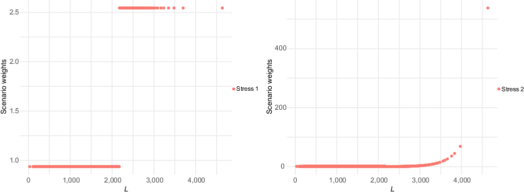
Next, we illustrate the difference between the two stresses applied, by a scatter plot of the scenario weights against the portfolio loss L. As the number of scenario weights is large, we only plot 5,000 data points. This can be achieved via the parameter n in the function plot_weights, that has a default of $n = 5,000$ .

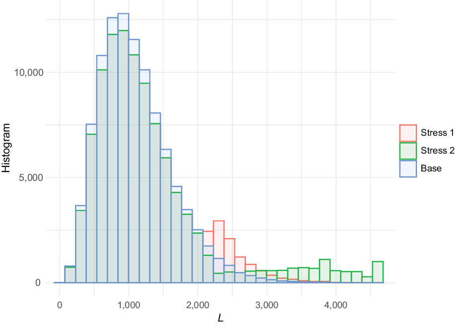
It is seen in Figure 6 that the weights generated to stress VaR, and VaR and ES together, follow different patterns to the weights used to stress means and standard deviations, as shown in section 2. Recall that SWIM calculates the scenario weights such that under the stressed model the given constraints are fulfilled. Thus, an increase in the VaR and/or ES of the portfolio loss L results in large positive realisations of L being assigned higher weight. On the other hand, when the standard deviation is stressed, scenario weights are calculated that inflate the probabilities of both large positive and negative values. When we compare stress 1 and stress 2 in Figure 6, we see that stressing VaR induces a high but constant weight on scenarios that correspond to large outcomes of L, while when stressing VaR and ES, the weights are exponentially increasing in (tail observations of) L. This difference in pattern is associated with the different impacts on the shape of the tail of L.

Figure 6

Scenario weights against the portfolio loss L for stressing VaR (left) and stressing both VaR and ES (right).

Figure 7

Histogram of the portfolio loss L under the baseline and the two stressed models.

4.4 Visualising stressed distributions

The change in the distributions of the portfolio and subportfolio losses, when moving from the baseline to the stressed models, can be visualised through the functions plot_hist and plot_cdf. The following figure displays the histogram of the aggregate portfolio loss under the baseline and the two stressed models. It is seen how stressing VaR and ES has a higher impact on the right tail of L, compared to stressing VaR only, see Figure 7. This is consistent with the tail-sensitive nature of the Expected Shortfall risk measure (McNeil et al., Reference McNeil, Frey and Embrechts2015). Moreover, the discontinuity in the way that, for stress 1, values of L map to the weights W, as seen in Figure 6, makes the stressed density of L no longer monotonic in the tail. These observations indicate that stressing both VaR and ES together may be a preferable option for risk management applications.

The arguments xCol and wCol (with default to plot all stresses) define the columns of the data and the columns of the scenario weights, respectively, that are used for plotting. Next, we analyse the impact that stressing the aggregate loss L has on the subportfolios $L_1, L_2, L_3$ . Again, we use the function plot_hist and plot_cdf for visual comparison, but this time placing the distribution plots and histograms of subportfolio losses along each other via the function ggarrange (from the package ggpubr). The plots obtained from plot_hist and plot_cdf can be further customised when specifying the argument displ = FALSE, as then the graphical functions plot_hist and plot_cdf return data frames compatible with the package ggplot2.

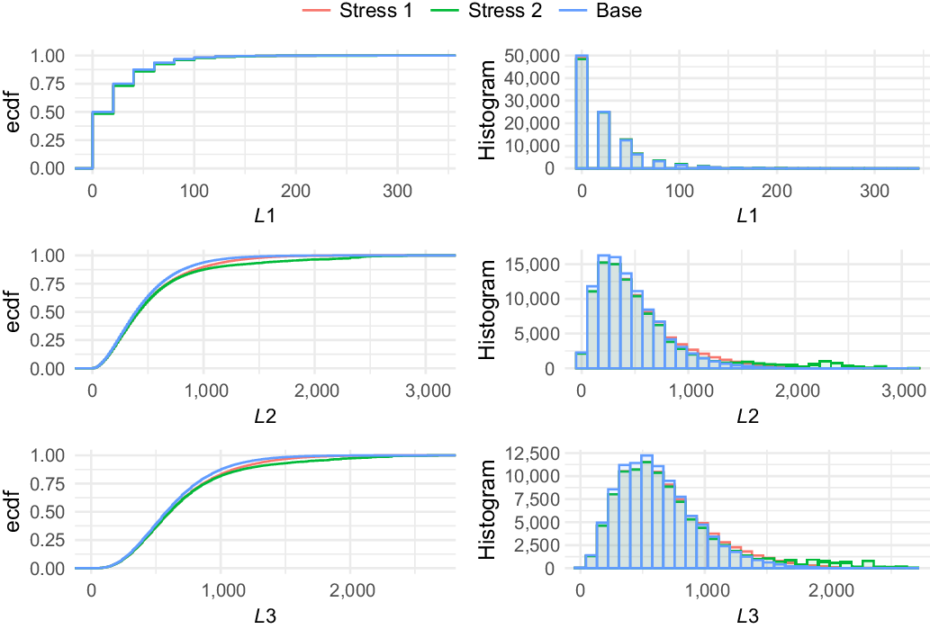
It is seen from both the distribution plots and the histograms in Figure 8 that the stresses have no substantial impact on $L_1$ , while $L_2$ and $L_3$ are more affected, indicating a higher sensitivity. Specifically, the distributions of $L_1$ under the baseline model and the two stresses are visually indistinguishable. This indicates the lack of importance of $L_1$ with respect to portfolio tail risk. The higher impact on the tails of stress 2 (on both VaR and ES) is also visible. Sensitivity measures quantifying these effects are introduced in the following subsection.

Figure 8

Distribution functions and histograms of the subportfolios $L_1, L_2, L_3$ for the stresses on the VaR (stress 1) and on both the VaR and ES (stress 2) of the portfolio loss L.

4.5 Sensitivity measures

The impact of the stressed models on the model components can be quantified through sensitivity measures. The function sensitivity includes the Kolmogorov distance, the Wasserstein distance, and the sensitivity measure Gamma; the choice of measure is by the argument type. We refer to section 3.2 for the definitions of those sensitivity measures. The Kolmogorov distance is useful for comparing different stressed models. Calculating the Kolmogorov distance, we observe that stress 2 produces a larger Kolmogorov distance compared to stress 1, which reflects the additional stress on the ES for the stressed model stress 2.

We now rank the sensitivities of model components by the measure Gamma, for each stressed model. Consistently with what the distribution plots showed, $L_2$ is the most sensitive subportfolio, followed by $L_3$ and $L_1$ . The respective default probabilities $H_1,H_2,H_3$ are similarly ranked.

Using the sensitivity function, we can analyse whether the sensitivity of the joint subportfolio $L_1 + L_3$ exceeds the sensitivity of the (most sensitive) subportfolio $L_2$ . This can be accomplished by specifying, through the argument f, a list of functions applicable to the columns k of the dataset. By setting xCol = NULL, only the transformed data are considered. The sensitivity measure of functions of columns of the data is particularly useful when high-dimensional models are considered, providing a way to compare the sensitivity of blocks of model components.

We observe that the sensitivity of $L_1 + L_3$ is larger than the sensitivity to either $L_1$ and $L_3$ , reflecting the positive dependence structure of the credit risk portfolio. Nonetheless, subportfolio $L_2$ has not only the largest sensitivity compared to $L_1$ and $L_3$ but also a higher sensitivity than the combined subportfolios $L_1 + L_3$ . This has a clear risk management implication, as it shows conclusively that $L_2$ should be an area of priority for the owner of this portfolio of credit liabilities. Loosely speaking, $L_2$ is the portfolio from which “problems may arise”.

The importance_rank function, having the same structure as the sensitivity function, returns the ranks of the sensitivity measures. This function is particularly useful when several risk factors are involved.

4.6 Constructing more advanced stresses

4.6.1 Sensitivity of default probabilities

From the preceding analysis, it transpires that the subportfolios $L_2$ and $L_3$ are, in that order, most responsible for the stress in the portfolio loss, under both stresses considered. Furthermore, most of the sensitivity seems to be attributable to the systematic risk components $H_2$ and $H_3$ , reflected by their high values of the Gamma measure. To investigate this, we perform another stress, resulting once again in a 20% increase in $\text{VaR}(L)$ , but this time fixing some elements of the distribution of $H_2$ . Specifically, in addition to the 20% increase in $\text{VaR}(L)$ , we fix the mean and the 75% quantile of $H_2$ to the same values as in the baseline model. Hence, we once again perform a reverse stress test, but this time intentionally restricting the movement in the distribution of $H_2$ , to enable us to focus on other variables. This set of constraints is implemented via the function stress_moment.

Using the summary function, we verify that the distribution of $H_2$ under the new stress has unchanged mean and 75th quantile. Then, we compare the sensitivities of the subportfolio losses under all three stresses applied.

It is seen that, by fixing part of the distribution of $H_2$ , the importance ranking of the subportfolios changes, with $L_2$ now being significantly less sensitive than $L_3$ . This confirms, in the credit risk model, the dominance of the systematic risk, reflected in the randomness of default probabilities.

4.6.2 Stressing tails of subportfolios

Up to now, we have considered the impact of stressing the aggregate portfolio loss on subportfolios. Now, following a forward sensitivity approach, we consider the opposite situation: stressing the subportfolio losses and monitoring the impact on the aggregate portfolio loss L. First, we impose a stress requiring a simultaneous 20% increase in the 90th quantile of the losses in subportfolios $L_2$ and $L_3$ . Note that the function stress_VaR (and stress_VaR_ES) allow to stress the VaR and/or the ES of only one model component. Thus, to induce a stress on the 90th quantiles of $L_2$ and $L_3$ , we use the function stress_moments and interpret the quantile constraints as moment constraints, via $E(1_{L_2 \leq \text{VaR}^W(L_2)})$ and $E(1_{L_3 \leq \text{VaR}^W(L_3)})$ , respectively, where $\text{VaR}^W = \text{VaR} \cdot 1.2$ denotes the VaRs in the stressed model.

It is seen how the stressing of subportfolios $L_2$ and $L_3$ has a substantial impact on the portfolio loss. Given the importance of dependence for the distribution of the aggregate loss of the portfolio, we strengthen this stress further, by additionally requiring that the frequency of joint high losses from $L_2$ and $L_3$ is increased. Specifically, we require the joint exceedance probability to be $P^W(L_2 > VaR^W(L_2), L_3 > VaR^W(L_3)) = 0.06$ , which is almost doubling the corresponding probability in the last stressed model, which was equal to 0.0308.

## [1] 0.00865

## [1] 0.0308

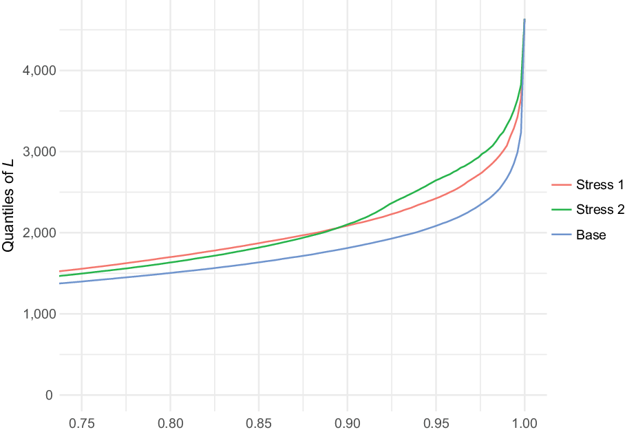
We analyse the impact the stresses of the tail of the subportfolios $L_2$ and $L_3$ have on the aggregate portfolio L. For this, we plot in Figure 9 the quantile of the aggregate portfolio under the baseline model (blue), under the stress on the tail of $L_2$ and $L_3$ (red), and under the additional stress on the joint tail of $L_2$ and $L_3$ (green).

The results and the plots indicate that the additional stress on joint exceedances of subportfolios increases the tail quantiles of L even further, demonstrating the importance of (tail-)dependence in portfolio risk management.

Figure 9

Quantiles of the aggregate loss L under the baseline (blue), the stress on the tails of $L_2$ and $L_3$ (red), and the additional stress on the joint tail of $L_2$ and $L_3$ (green).