I. INTRODUCTION
Beamforming is a signal processing technique used to control the directionality of the transmission and reception of the radio signals [Reference Schlieter and Eigenbrod1]. This is achieved by distributing the elements of the array in such a way that signals at a particular angle experience constructive interference, whereas others experience destructive interference. Beamforming can be used at both transmitting and receiving ends in order to achieve spatial selectivity. Hyper beamforming [Reference Anita, Sri Jaya Lakshmi, Sreedevi, Khan, Sarat Kumar and Ramakrishna2] refers to the spatial processing algorithm used to focus an array of spatially distributed elements (called sensors) to increase the signal-to-interference plus noise ratio (SINR) at the receiver. This beamforming processing improves significantly the gain of the wireless link over a conventional technology, thereby increasing range, rate, and penetration [Reference Isernia, Ares Pena, Bucci, Durso, Gomez and Rodriguez3–Reference Takao and Komiyama5]. It has found numerous applications in radar, sonar, seismology, wireless communication, radio astronomy, acoustics, and biomedicine [Reference Schilter6]. It is generally classified as either conventional (switched and fixed) beamforming or adaptive beamforming. Switched beamforming system [Reference Balanis7, Reference Krous8] is a system that can choose one pattern from many predefined patterns in order to enhance the received signals. Fixed beamforming uses a fixed set of weights and time delays (or phasing) to combine the signals received from the sensors in the array, primarily using only information about the locations of the sensors in space and the wave direction of interest [Reference Anita, Sri Jaya Lakshmi, Sreedevi, Khan, Sarat Kumar and Ramakrishna2]. Adaptive beamforming or phased array is based on the desired signal maximization mode and interference signal minimization mode [Reference Mailloux9–Reference Applebaum and Chapman11]. It is able to place the desired signal at the maximum of the main lobe. Hyper beamforming/any other beamforming offers high detection performance such as beamwidth, target-bearing estimation and reduces false alarm, sidelobe suppression. A new optimized hyper beamforming technique is presented in this paper, and the Firefly algorithm (FFA) is applied to obtain optimal hyper beam patterns of linear antenna arrays.
The classical gradient-based optimization methods are not suitable for optimal design of hyper beamforming of linear antenna arrays because of the following reasons: (i) highly sensitive to the starting points when the number of solution variables and hence the size of the solution space increase, (ii) frequent convergence to local optimum solution or divergence or revisiting the same suboptimal solution, (iii) requirement of continuous and differentiable objective function, (iv) requirement of the piecewise linear cost approximation (linear programming), and (v) problem of convergence and algorithm complexity (non-linear programming). Hence, evolutionary methods have been employed for the optimal design of hyper beamforming of linear antenna arrays with better parameter control.
Different evolutionary optimization algorithms such as simulated annealing algorithm [Reference Chen12], genetic algorithm (GA) [Reference Haupt13–Reference Eberhart and Shi17] etc. have been widely used for the synthesis of design methods capable of satisfying the constraints. When considering the global optimization methods for antenna arrays design, GA seems to be the promising one. Although standard GA [here referred to as real-coded genetic algorithm (RGA)] has a good performance for finding the promising regions of the search space, however, finally, the RGA is prone to revisiting the same suboptimal solutions.
Particle swarm optimization (PSO) is an evolutionary algorithm developed by Kennedy and Eberhart [Reference Kennedy and Eberhart18]. PSO is simple to implement and its convergence may be controlled via a few parameters [Reference Mandal, Yallaparagada, Ghoshal and Bhattacharjee19–Reference Van den Bergh and Engelbrecht27]. The limitations of the conventional PSO are that it may be influenced by premature convergence and stagnation problem.
The Differential evolution (DE) algorithm was first introduced by Storn and Price in 1995 [Reference Storn and Price28]. Like the RGA, it is a randomized stochastic search technique enriched with the operations of crossover, mutation and selection [Reference Storn and Price29–Reference Mandal, Ghoshal, Kar and Mandal39] and prone to premature convergence and stagnation. Hence, to enhance the performance of the optimization algorithms in global search (exploration stage) as well as local search (exploitation stage), an alternative technique such as FFA [Reference Yang40–Reference Yang44] has been suggested for the optimization of hyper beamforming in this paper.
The rest of the paper is arranged as follows. In Section II, the design equations of hyper beamforming of linear antenna array are formulated. Section III briefly discusses the evolutionary techniques RGA, PSO, DE, and FFA employed for the designs of linear antenna arrays. Section IV describes the simulation results obtained by using the techniques. Finally, Section V concludes the paper.
II. DESIGN EQUATIONS
In hyper beamforming for linear antenna array the inter-element spacing of λ/2 in either direction is considered. The sum beam can be created by summation of the absolute values of complex left and right half beams, as shown in Fig. 1. The difference beam is the absolute magnitude of the difference of complex right beam half beam and left half beam signals. Furthermore, the difference beam has a minimum in the direction of the sum beam at zero degree as shown in Fig. 2. The resulting hyper beam is obtained by subtraction of the sum and the difference beams, each raised to the power of the exponent u.
Sum beam pattern for the 10-element linear array for u = 1.

Difference beam pattern for the 10-element linear array for u = 1.
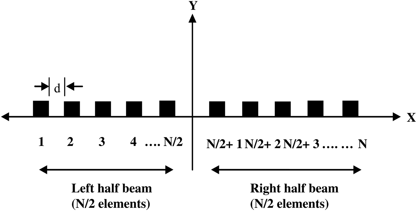
Consider a broadside linear array of N equally spaced isotropic elements as shown in Fig. 3. The array is symmetric in both geometry and excitation with respect to the array center [Reference Anita, Sri Jaya Lakshmi, Sreedevi, Khan, Sarat Kumar and Ramakrishna2].
Geometry of an N-element linear array along the x-axis.
For broadside beams, the array factor is given in (1) [Reference Balanis7].
 $$AF\lpar \theta \rpar =\sum\limits_{n=1}^N {I_n } e^{j\lpar n - 1\rpar K_d \lsqb \sin \theta \cos \varphi - \sin \theta _0 \cos \varphi _0 \rsqb }\comma \;$$
where θ is the angle of radiation of electromagnetic plane wave; θ 0 is the angle where the highest maximum of the angle is attained in θ ∈ [−π/2, π/2]; d is the spacing between elements; K is the propagation constant; N is thetotal number of elements in the array; and I n is the excitation amplitude of the nth element.
In this case, for the linear antenna arrays ϕ 0 = 0. The equations for the creation of the sum, difference and simple hyper beam patterns in terms of two half beams are as follows (2)(3) [Reference Anita, Sri Jaya Lakshmi, Sreedevi, Khan, Sarat Kumar and Ramakrishna2]:
 $${\rm Sum \;pattern}\comma \; Sum\lpar \theta \rpar =\left\vert {R_L } \right\vert +\left\vert {R_R } \right\vert \semicolon \; $$
 $${\rm Difference \;pattern}\comma \; Diff\lpar \theta \rpar =\left\vert {R_L - R_R } \right\vert \semicolon \; $$
where
 $$R_L=\sum\limits_{n=1}^{N/2} {I_n } e^{j\lpar n - 1\rpar K_d \lsqb \sin \theta \cos \varphi - \sin \theta _0 \cos \varphi _0 \rsqb }\comma \;$$
 $$R_R=\sum\limits_{n=N/2\, +\, 1}^N {I_n } e^{j\lpar n - 1\rpar K_d \lsqb \sin \theta \cos \varphi - \sin \theta _0 \sin \varphi _0 \rsqb }.$$
The hyper beam is obtained by subtraction of the sum and difference beams, each raised to the power of the exponent u; the general equation of the hyper beam is a function of the hyper beam exponent u given in (4) [Reference Anita, Sri Jaya Lakshmi, Sreedevi, Khan, Sarat Kumar and Ramakrishna2].
 $$AF_{Hyper} \lpar \theta \rpar =\left\{{\left({\left\vert {R_L } \right\vert +\left\vert {R_R } \right\vert } \right)^u - \left({\left\vert {R_L - R_R } \right\vert } \right)^u } \right\}^{1/u}\comma \; $$
where u ranges from 0.2 to 1. If u lies below 0.2, the hyper beam pattern will contain a large spike height at the peak of the main beam without changing the overall hyper beam pattern. If u is more than 1, the sidelobes of the hyper beam will be more as compared to those of the conventional radiation pattern.
All of the antenna elements are assumed to be isotropic. Only amplitude excitations and inter-element spacing are used to change the antenna radiation pattern. The cost function (J) for improving the sidelobe level (SLL) of the radiation pattern of the hyper beam linear antenna arrays is given in (5).
 $$\eqalign{J &= Max \vert {AF_{Hyper} \lpar \theta _{msl1}\comma \; I_n \rpar } \vert / \vert AF_{Hyper} \lpar \theta _0\comma \; I_n \rpar \vert \cr &\quad + Max \vert AF_{Hyper} \lpar \theta _{msl2}\comma \; I_n \rpar \vert / \vert AF_{Hyper} \lpar \theta _0\comma \; I_n \rpar \vert.} $$
θ msl1 is the angle where the maximum sidelobe AF Hyper(θ msl1, I n) is attained in the lower band of the hyper beam pattern. θ msl2 is the angle where the maximum sidelobe AF Hyper(θ msl2, I n) is attained in the upper side band of the hyper beam pattern. In J, both the numerator and the denominator are in absolute magnitude. Minimization of J means maximum reduction of SLL. RGA, PSO, DE, and FFA are employed individually for minimization of J by optimizing the current excitation weights of the elements and inter-element spacing. Results of the minimization of J and SLL are described in Section IV.
III. OPTIMIZATION TECHNIQUES EMPLOYED
A) Real coded genetic algorithm
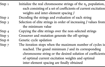
RGA is mainly a probabilistic search technique, based on the principles of natural selection and evolution. At each generation, it maintains a population of individuals where each individual is a coded form of a possible solution of the problem at hand called chromosome. Chromosomes are constructed over some particular alphabet, e.g., the binary alphabet {0, 1}, so that chromosomes' values are uniquely mapped onto the real decision variable domain. Each chromosome is evaluated by a function known as cost function, which is usually the objective function of the corresponding optimization problem [Reference Haupt13–Reference Eberhart and Shi17]. The basic steps of RGA are shown in Table 1.
Steps for the RGA.
B) Particle swarm optimization
PSO is a flexible, robust population-based stochastic search or optimization technique with implicit parallelism, which can be easily handled with non-differential objective functions, unlike traditional gradient-based optimization methods. PSO is less susceptible to getting trapped on local optima unlike GA, simulated annealing, etc. Kennedy and Eberhart [Reference Kennedy and Eberhart18] developed a PSO concept similar to the behavior of a swarm of birds [Reference Mandal, Yallaparagada, Ghoshal and Bhattacharjee19–Reference Van den Bergh and Engelbrecht27]. PSO is developed through a simulation of bird flocking and fish schooling in multi-dimensional space. Bird flocking optimizes a certain objective function. Each particle knows its best value so far (pbest). This information corresponds to the personal experiences of each particle. Moreover, each particle knows the best value so far in the group (gbest) among all of the pbests. Namely, each particle tries to modify its position using the following information:
• The distance between the current position and the pbest.
• The distance between the current position and the gbest.
Mathematically, the velocities of the vectors are modified according to the following equation:
 $$\eqalign{V_i^{k+1}&= CFa \times \lpar w^{k+1} \;\ast\; V_i^k+C_1 \;\ast\; rand_1 \;\ast\; \lpar pbest_i - S_i^k \rpar \cr &\quad +C_2 \;\ast\; rand_2 \;\ast\; \lpar gbest^k - S_i^k \rpar \rpar \comma \; }$$
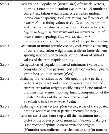
where V ik is the velocity of vector i at iteration k; w is the weighting function; C 1 and C 2 are called social and cognitive constants, respectively; rand i is the random number between 0 and 1; S ik is the current position of vector i at iteration k; pbest i is the pbest of vector i; gbest k is the gbest of the group of vectors at iteration k. The first term of (6) is the previous velocity of the vector. The second and third terms are used to change the velocity of the vector. Without the second and third terms, the vector will keep “flying” in the same direction until it hits the boundary. The parameter w corresponds to a kind of inertia and tries to explore new areas. Here, the vector is termed for the string of real current excitation weight coefficients (N number) and uniform inter-element spacing (01 number). Total variables = nvar = N + 1 in each vector. Normally, C 1 = C 2 = 1.5–2.05 and the Constriction Factor (CFα)is given in (7).
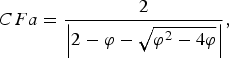 $$CFa=\displaystyle{2 \over {\left\vert {2 - \varphi - \sqrt {\varphi ^2 - 4\varphi } } \right\vert }}\comma \; $$
where
 $$\varphi=C_1+C_2 \quad {\rm and}\quad \varphi\gt 4. $$
For C 1 = C 2 = 2.05, the computed value of CFα = 0.73.
The best values of C 1, C 2, and CFα are found to vary with the design sets (Table 2).
Steps for PSO.
Inertia weight (w k+1) at (k + 1)th cycle is given in (9).
 $$w^{k+1}=w_{max} - \displaystyle{{w_{max} - w_{min} } \over {k_{max} }} \times \lpar k+1\rpar \comma \;$$
where w max = 1.0; w min = 0.4; k max = maximum number of iteration cycles. The searching point/updated vector in the solution space can be modified by (10).
 $$S_i^{k+1}=S_i^k+V_i^{k+1}.$$
C) DE algorithm
The crucial idea behind the DE algorithm [Reference Storn and Price28–Reference Mandal, Ghoshal, Kar and Mandal39] is a scheme for generating trial parameter vectors and adds the weighted difference between two population vectors to a third one. Like any other evolutionary algorithm, the DE algorithm aims at evolving a population of N P, D-dimensional parameter vectors, so-called individuals, which encode the candidate solutions, i.e.,
 $$\overrightarrow {x_{i\comma g} }=\left\{{x_{1\comma i\comma g}\comma \; x_{2\comma i\comma g}\comma \; ...\comma \; x_{D\comma i\comma g} } \right\}\comma \;$$
where i = 1, 2, 3,…, N P. The initial population (at g = 0) should cover the entire search space as much as possible by uniformly randomizing the individuals within the search constrained by the prescribed minimum and maximum parameter bounds:  $\vec{x} _{min}=\left\{{x_{1\comma min}\comma \; ...\comma \; x_{D\comma min} } \right\}$ and
 $\vec{x} _{max}=\left\{{x_{1\comma max}\comma \; ...\comma \; x_{D\comma max} } \right\}.$
For example, the initial value of the jth parameter of the ith vector is
 $$x_{j\comma i\comma 0}=x_{j\comma min}+rand\left({0\comma \; 1} \right)\;\ast\; \left({x_{j\comma \max } - x_{j\comma min} } \right)\comma \;$$
where j = 1, 2, 3,…, D.
The random number generator, rand (0,1), returns a uniformly distributed random number from within the range [0,1]. After initialization, DE enters a loop of evolutionary operations: mutation, crossover, and selection.
1) MUTATION
Once initialized, DE mutates and recombines the population to produce new population. For each trial vector x i, g at generation g, its associated mutant vector  $\vec v _{i\comma g}=\left\{{v_{1\comma i\comma g}\comma \; v_{2\comma i\comma g}\comma \; ...\comma \; v_{D\comma i\comma g} } \right\}$ can be generated via a certain mutation strategy. Five most frequently used mutation strategies in the DE codes are listed as follows:
 $$" DE/rand/1 " \colon \vec v _{i\comma g}=\vec{x} _{r_1^{\prime}\comma g}+F\left({\vec{x} _{r_2^{\prime}\comma g} - \vec{x} _{r_3^{\prime}\comma g} } \right)\comma \;$$
 $$"DE/best/1 " \colon \vec v _{i\comma g}=\vec{x} _{best\comma g}+F\left({\vec{x} _{r_1^{\prime}\comma g} - \vec{x} _{r_2^{\prime}\comma g} } \right)\comma \;$$
 $$\eqalign{"DE/rand - to - best/1 " \colon \vec v _{i\comma g} & =\vec{x} _{i\comma g}+F\left({\vec{x} _{best\comma g} - \vec{x} _{i\comma g} } \right)\cr & \quad+F\left({\vec{x} _{r_1^{\prime}\comma g} - \vec{x} _{r_2^{\prime}\comma g} } \right)\comma \; }$$
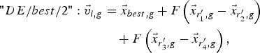 $$\eqalign{"DE/best/2 " \colon \vec v _{i\comma g} & =\vec{x} _{best\comma g}+F\left({\vec{x} _{r_1^{\prime}\comma g} - \vec{x} _{r_2^{\prime}\comma g} } \right)\cr &\quad +F\left({\vec{x} _{r_3^{\prime}\comma g} - \vec{x} _{r_4^{\prime}\comma g} } \right)\comma \; }$$
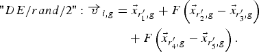 $$\eqalign{"DE/rand/2 " \colon \overrightarrow v _{i\comma g} & =\vec{x} _{r_1^{\prime}\comma g}+F\left({\vec{x} _{r_2^{\prime}\comma g} - \vec{x} _{r_3^{\prime}\comma g} } \right)\cr & \quad+F\left({\vec{x} _{r_4^{\prime}\comma g} - \vec{x} _{r_5^{\prime}\comma g} } \right).}$$
The indexes r 1′, r 2′, r 3′, r 4′, and r 5′ are mutually exclusive integers randomly chosen from the range [1, N P], and all are different from the base index i. These indexes are randomly generated once for each mutant vector. The scaling factor F is a positive control parameter for scaling the difference vector. x best,g is the best individual vector with the best fitness value in the population at generation “g”. In the present work, (15) has been used.
2) CROSSOVER
To complement the differential mutation search strategy, a crossover operation is applied to increase the potential diversity of the population. The mutant vector v i,g exchanges its components with the target vector x i,g to generate a trial vector:
 $$\vec{u} _{i\comma g}=\left\{{u_{1\comma i\comma g}\comma \; u_{2\comma i\comma g}\comma \; ...\comma \; u_{D\comma i\comma g} } \right\}.$$
In the basic version, DE employs the binomial (uniform) crossover defined as
 $$u_{j,i,g}=\left\{\matrix{v_{j,i,g}, \hfill & {\rm if} (rand_{i,j}(0,1)\leq C_{r} \, {\rm or}\, j \, =j_{rand}),\cr x_{i,j,g}, \hfill & \hfill {\rm otherwise},}\right.$$
where j = 1, 2,…, D.
The crossover rate C r is user-specified constant within the range (1,0), which controls the fraction of parameter values copied from the mutant vector. j rand is a randomly chosen integer in the range [1,D]. The binomial crossover operator copies the jth parameter of the mutant vector  $\vec v _{i\comma g}$ to the corresponding element in the trial vector
 $\vec{u} _{i\comma g}$ if rand i,j(0,1) ≤ C r or j = j rand. Otherwise, it is copied from the corresponding target vector
 $\vec{x} _{i\comma g}$.
3) SELECTION
To keep the population size constant over subsequent generations, the next step of the algorithm calls for selection to determine whether the target or the trial vector survive to the next generation, i.e., at g = g + 1. The selection operation is described in (20):
 $$\vec{x} _{i\comma g+1}=\left\{\matrix{\vec{u} _{i\comma g}\comma \; \hfill &{\rm if }\;f\left(\vec{u} _{i\comma g} \right) \leq f\left(\vec{x} _{i\comma g} \right)\comma \; \cr \vec{x} _{i\comma g} \comma \; \hfill &\quad\quad\quad\quad{\rm otherwise}\comma \;} \right.$$
where f (x) is the J (in this work) to be minimized. Hence, if the new vector yields an equal or lower value of J, it replaces the corresponding target vector in the next generation; otherwise, the target is retained in the population. Hence, the population either gets better (with respect to the minimization of the cost function) or remains the same in fitness status, but never deteriorates.
The above three steps are repeated generation after generation until some specific termination criteria are satisfied.
4) CONTROL PARAMETER SELECTION OF DE
Proper selection of control parameters is very important for the success and performance of an algorithm. The optimal control parameters are problem-specific. Therefore, the set of control parameters that best fit each problem have to be chosen carefully. Values of F lower than 0.3 may result in premature convergence, while values greater than 1 tend to slow down the convergence speed. Large populations help maintain diverse individuals, but also slow down convergence speed. In order to avoid premature convergence, F or N P should be increased or C r should be decreased. Larger values of F result in larger perturbations and better probabilities to escape from the local optima, while lower C r preserves more diversity in the population, thus avoiding the local optima.
5) Algorithmic description of DE
Step 1. Generation of initial population: Set the generation counter g = 0 and randomly initialize the D-dimensional N p individuals (parameter vectors/target vectors),  $\vec{x} _{i\comma g}=\left\{{x_{1\comma i\comma g}\comma \; x_{2\comma i\comma g}\comma \; ...\comma \; x_{D\comma i\comma g} } \right\}\comma$ where i = 1,2,3,…,N P. The initial population (at g = 0) should cover the entire search space as much as possible by uniformly randomizing the individuals within the search constrained by the prescribed minimum and maximum parameter bounds:
 $\vec{x} _{min}=\left\{{x_{1\comma min}\comma \; ...\comma \; x_{D\comma min} } \right\}$ and
 $\vec{x} _{max}=\left\{{x_{1\comma max}\comma \; ...\comma \; x_{D\comma max} } \right\}.$
Step 2. Mutation: For i = 1 to N P, generate a mutated vector,  $\vec v _{i\comma g}=\left\{{v_{1\comma i\comma g}\comma \; v_{2\comma i\comma g}\comma \; ...\comma \; v_{D\comma i\comma g} } \right\}$ corresponding to the target vector
 $\vec{x} _{i\comma g}$ via mutation strategy (15).
Step 3. Crossover: Generation of a trial vector  $\vec{u} _{i\comma g}$ for each target vector
 $\vec{x} _{i\comma g}$, where
 $\vec{u} _{i\comma g}=\left\{{u_{1\comma i\comma g}\comma \; u_{2\comma i\comma g}\comma \; ...\comma \; u_{D\comma i\comma g} } \right\}$.
for i = 1 to N P; j rand = [rand(0,1)*D]; for j = 1 to D.
 $$u_{j\comma i\comma g}=\left\{\matrix{v_{j\comma i\comma g } \comma \;\hfill &{\rm if } \;\left(rand_{i\comma j} \;\left(0\comma \; 1 \right) \leq C_r \;{\rm or }\;j = j_{rand} \right)\comma \; \cr x_{i\comma j\comma g}\comma \;\hfill &\quad\quad\quad\quad\quad\quad\quad\qquad{\rm otherwise} .} \right.$$
Step 4. Selection: for i = 1 to N P,
 $$\vec{x} _{i\comma g+1}=\left\{\matrix{\vec{u} _{i\comma g}\comma \; \hfill &\;{\rm if }f\left(\vec{u} _{i\comma g} \right) \leq f\left(\vec{x} _{i\comma g} \right)\comma \; \cr \vec{x} _{i\comma g} \comma \; \hfill &\quad\quad\quad\quad{\rm otherwise} .} \right.$$
Increment the generation count g = g + 1.
D) Firefly algorithm
FFA, developed by Yang [Reference Yang40], is inspired by the flash pattern and characteristics of fireflies. The basic rules for the FFA are:
• All of the fireflies are unisex so that one firefly will be attracted to other fireflies regardless of their sex.
• Attractiveness is proportional to their brightness, thus for any two flashing fireflies, the less bright one will move toward the brighter one, and the brightness decreases as their distance increases. If there is no brighter one than a particular firefly, it will move randomly.
• The brightness of a firefly is affected or determined by the landscape of the cost function. For a minimization problem, the brightness can simply be inversely proportional to the value of the cost function. In this work, the cost function is J.
In the simplest case for the minimization optimization problems, the brightness B of a firefly at a particular location x can be chosen as B(x) = 1/f(x), where f(x) is J in this work. However, the attractiveness β is relative; it should be seen in the eyes of the beholder or judged by the other fireflies. Thus, it will vary with the distance r ij between firefly i and firefly j. For a given medium with a fixed light absorption coefficient,γ, the light intensity varies with the distance r. That is
 $$B=B_0 e^{ - \gamma r}\comma \;$$
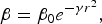
where B 0 is the original light intensity; r is the Euclidean distance between the fireflies. As a firefly's attractiveness is proportional to the light intensity seen by adjacent fireflies, the attractiveness/repulsiveness β of a firefly can be defined by
 $$\beta=\beta _0 e^{ - \gamma r^2 }\comma \;$$
where β 0 is the attractiveness (positive sign)/repulsiveness (negative sign) at r = 0.
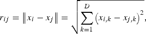
The distance between any two fireflies i and j at x i and x j, respectively, is the Euclidean distance.
 $$r_{ij}=\left\Vert {x_i - x_j } \right\Vert =\sqrt {\sum\limits_{k=1}^D {\left({x_{i\comma k} - x_{j\comma k} } \right)^2 } }\comma \;$$
where x i,k is the kth component of the special coordinate x i of the ith firefly; D is the dimension of each x i and x j.
The movement of a firefly i is attracted by another more attractive (brighter) firefly j or repelled by more repulsive (less bright) firefly j and is determined by
 $$x_i=x_i+\beta _0 e^{ - \gamma r_{ij}^2 } \lpar x_j - x_i \rpar +\alpha \left(rand - \displaystyle{1 \over 2} \right)$$
where the second term is due to the attraction or repulsion. The third term is randomized with a control parameter α, which makes the exploration of search space more efficient. Usually, β 0 = 1, α ∈ [0,1] for most applications. By adjusting the parameters γ, α and β 0, the performance of the algorithm can be improved.
Steps of FFA are as follows:
Step 1: Generate initial firefly vectors xi = (xi1,…,xiD) (i = 1,…,120), where D = N + 1 (N element excitations I ∈ [0,1] plus the common inter-element spacing d ∈ [λ/2,λ]). Set the maximum allowed number of iterations to 100. β 0 = 0.6, γ = 0.2, and α = 0.01 (these values, and the population size, 120, were determined as optimal in a series of 30 preliminary trials.
Step 2: Computation of initial J of the total population.
Step 3: Computation of the initial population based best solution (gbest) vector corresponding to the historical population best and least J value.
Step 4: Update the firefly positions:
(a) Compute the square root (rsqrt) of the Euclidean distance between the first particle vector and the second particle vector as per (23).
(b) Compute β with the help of β 0 as per (22).
(c) If J of second particle is <J of first particle, then, update the first particle as per (24) with +β 0 (case of attraction), otherwise with −β 0 (case of repulsion).
IV. NUMERICAL RESULTS
Each algorithm was run 100 times to get its best solutions. The best results are reported in this work. Population size chosen for RGA, PSO, DE, and FFA is 120. Best control parameters for the RGA are: Crossover rate = 0.8; Crossover taken is two point crossover; mutation rate = 0.05; type of mutation is Gaussian mutation; selection, probability = Roulette wheel, 1/3. Best control parameters for PSO are: C 1, C 2 = 1.5, 1.5; v imin, v imax = 0.01, 1.0; w max, w min = 1.0, 0.4. Best parameters for DE are: C r = 0.3; F = 0.5. Best parameters for FFA are: α,γ, β0 = 0.01, 0.2, 0.6. These best parameters have been determined after 30 trial runs of each algorithm.
A) Analysis of radiation patterns of hyper beam without optimization
This section gives the experimental results for various hyper beams of non-optimized linear antenna array designs. Three linear antenna array designs considered are of 10-, 14-, and 20-element sets, each maintaining uniform inter-element spacing. Reduction of main beam width [first null beam width (FNBW)] and SLL can be controlled by varying the hyper beam exponent value u, thereby obtaining different hyper beam patterns. The results show that the SLL reduction increases as the exponent value u decreases. For 10-, 14-, and 20-element linear arrays, with u = 1, SLL reductions are −19.91, −20.10, and −20.20 dB, respectively, whereas with u = 0.5, the SLL reduces to −32.78, −33.02, and −33.20 dB, respectively, as shown in Figs 4–9 and Table 3. The uniform linear array shows the respective SLL values as −12.97, −13.11, and −13.20 dB. Therefore, the optimization technique applied to the hyper beam yields much more reduction of SLL in comparison to that of the uniform linear array and non-optimized hyperbeam case. Main beam width (FNBW) remains unaltered or has been improved for all of the cases of FFA unlike RGA, DE, and PSO.
Best array pattern found by the FFA for the 10-element array with improved SLL and FNBW at u = 0.5.
Best array pattern found by the FFA for the 14-element array with improved SLL and FNBW at u = 0.5.
Best array pattern found by the FFA for the 20-element array with improved SLL and FNBW at u = 0.5.
Best array pattern found by the FFA for the 10-element array with improved SLL and FNBW at u = 1.
Best array pattern found by the FFA for the 14-element array with improved SLL and FNBW at u = 1.
Best array pattern found by the FFA for the 20-element array with improved SLL and FNBW at u = 1.
Initial values of SLL and FNBW for uniform linear array having uniform excitation (I n = 1) and d = λ/2 inter-element spacing.
B) Analysis of radiation patterns of hyper beam with optimization by RGA, PSO, DE, and FFA
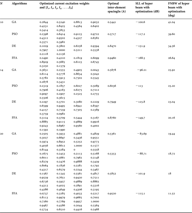
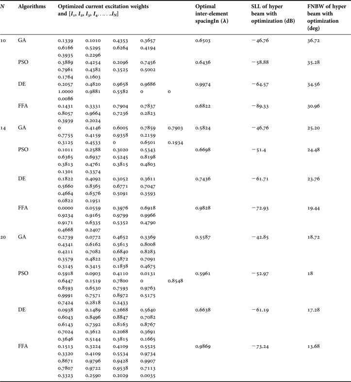
This section gives the experimental results for various optimized hyper beam antenna array designs obtained by the RGA, PSO, DE, and FFA techniques. The parameters of the RGA, PSO, DE, and FFA are set after many trial runs. It is found that the best results are obtained for the initial population (n p) of 120 chromosomes and maximum number of generations, Nm as 100. With the RGA, for selection operation, the method of natural selection is chosen with a selection probability of 0.3. Crossover is randomly selected as a dual point. The Crossover ratio is 0.8. Mutation probability is 0.05. Each RGA, PSO, DE, and FFA technique individually generates a set of optimized, non-uniform current excitation weights, and optimal uniform inter-element spacing for same three sets of linear antenna arrays. Tables 4 and 5 show the SLL, FNBW, and optimal current excitation weights with the hyper beam exponent values u = 0.5, and u = 1, respectively, for the optimally excited hyper beam linear antenna array with optimized uniform inter-element spacing (d ∈ [λ/2,λ]) using RGA, PSO, DE, and FFA. Figures 4–9 depict the radiation patterns of linear antenna arrays with the exponent values u = 0.5 and u = 1 for sets of 10, 14, and 20 number of elements, respectively, with optimized non-uniform excitations and optimized fixed inter-element spacing, as obtained by the techniques. Figures clearly show improvement of SLL and FNBW by optimization of hyper beam.
SLL, FNBW, optimal current excitation weights, and optimal inter-element spacing for hyper beam pattern of linear array with hyper beam exponent (u = 0.5), obtained by RGA, PSO, DE, and FFA for different sets of arrays.
SLL, FNBW, optimal current excitation weights, and optimal inter-element spacing for hyper beam pattern of linear array with hyper beam exponent (u = 1), obtained by RGA, PSO, DE, and FFA for different sets of arrays.
1) ANALYSIS OF RADIATION PATTERNS OF HYPER BEAM WITH U = 0.5 AND OPTIMIZATION BY RGA, PSO, DE, AND FFA
The following observations are made from Table 4, in which the exponent value u = 0.5. For the 10-element array, RGA, PSO, DE, and FFA yield SLL values −100.6, −117.2, −151.9, and −168.5 dB, respectively, of the optimized hyper beam pattern against the SLL of −32.78 dB of the non-optimized hyper beam pattern. Similarly, for the same array, RGA, PSO, DE, and FFA yield FNBW values 41.04°, 39.60°, 34.56°, and 26.64°, respectively, of the optimized hyper beam pattern against the FNBW of 33.12° of the non-optimized hyper beam pattern. For the 14-element array, RGA, PSO, DE, and FFA yield SLL values −96.21, −113, −125.8, and −149.7 dB, respectively, of the optimized hyper beam pattern against the SLL of −33.02 dB of the non-optimized hyper beam pattern. Similarly, for the same array, RGA, PSO, DE, and FFA yield FNBW values 25.92°, 25.20°, 23.04°, and 20.16°, respectively, of the optimized hyper beam pattern against the FNBW of 23.04° of the non-optimized hyper beam pattern. For the 20-element array, RGA, PSO, DE, and FFA yield SLL values −83.69, −88.71, −101.9, and −115.1 dB, respectively, of the optimized hyper beam pattern against the SLL of −33.20 dB of the non-optimized hyper beam pattern. Similarly, for the same array, RGA, PSO, DE, and FFA yield FNBW values 19.44°, 18.72° and 18°, 11.52°, respectively, of the optimized hyper beam pattern against the FNBW of 16.56° of the non-optimized hyper beam pattern. The figures as well as Tables clearly show improvement of the SLL and FNBW by FFA-based optimization.
2) ANALYSIS OF RADIATION PATTERNS OF HYPER BEAM WITH U = 1 AND OPTIMIZATION BY RGA, PSO, DE, AND FFA
The following observations are made from Table 5, in which the exponent value u = 1. For the 10-element array, RGA, PSO, DE, and FFA yield SLL values −46.76, −58.88, −64.57, and −89.33 dB, respectively, of the optimized hyper beam pattern against the SLL of −19.91 dB of the non-optimized hyper beam pattern. Similarly, for the same array, RGA, PSO, DE, and FFA yield FNBW values 36.72, 35.28, 34.56, and 30.96°, respectively, of the optimized hyper beam pattern against the FNBW of 33.12° of the non-optimized hyper beam pattern. For the 14-element array, RGA, PSO, DE, and FFA yield SLL values −46.76, −51.4, −61.71, and −72.93 dB, respectively, of the optimized hyper beam pattern against the SLL of −20.10 dB of the non-optimized hyper beam pattern. Similarly, for the same array, RGA, PSO, DE, and FFA yield FNBW values 25.20°, 24.48°, 23.76°, and 19.44°, respectively, of the optimized hyper beam pattern against the FNBW of 23.04° of the non-optimized hyper beam pattern. For the 20-element array, RGA, PSO, DE, and FFA yield SLL values −42.85, −52.97, −61.19, and −73.24 dB, respectively, of the optimized hyper beam pattern against the SLL of −20.20 dB of the non-optimized hyper beam pattern. Similarly, for the same array, RGA, PSO, DE, and FFA yield FNBW values 18.72°, 18°, 17.28°, and 13.68°, respectively, of the optimized hyper beam pattern against the FNBW of 16.56° of the non-optimized hyper beam pattern. The figures as well as Tables clearly depict improvement of the SLL and FNBW by FFA-based optimization.
The FFA efficiently computes N number of near global optimal current excitation weights and one number optimal uniform inter-element separation for each hyper beam linear antenna array to have maximum SLL reduction and improved FNBW.
V. COMPARATIVE EFFECTIVENESS AND CONVERGENCE PROFILE OF RGA, PSO, DE, AND FFA
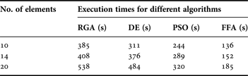
The algorithms can be compared in terms of the J values, Figs 10 and 11 show the convergences of the log10 (J) values obtained as RGA, PSO, DE, and FFA are employed, respectively. As compared to RGA, PSO, and DE which yield suboptimal higher values of J, the FFA converges to the least minimum J values in finding the near-global optimal current excitation weights and optimal inter-element spacing of the hyper beam of the antenna arrays. With a view to the above fact, it may finally be inferred that the performance of the FFA algorithm is the best among the algorithms. Figures 10 and 11 portray the convergence profiles of minimum J for the 10-element array sets, for u = 0.5 and 1, respectively. Table 6 shows the execution times of RGA, PSO, DE, and FFA. From the same table it is clear that the execution times of the FFA are all less than those of RGA, PSO, and DE. The simulation programming was performed in MATLAB language using MATLAB 7.5 on a dual core (TM) processor, 2.88 GHz with 2 GB RAM.
Convergence profile of the FFA in case of 10-element linear antenna array at u = 0.5.
Convergence profile of the FFA in case of 10-element linear antenna array at u = 1.
Comparison of execution times for different algorithms for different sets of elements.
VI. CONCLUSIONS
In this paper, a novel FFA is used for finding the optimal sets of non-uniformly excited (0 < I n ≤ 1) hyper beamforming of receiving linear antenna arrays, each with optimal uniform inter-element spacing (λ/2 ≤ d < λ).Three broad cases of arrays are considered in the study. The first two cases are: (i) conventional uniformly excited (I n = 1) linear antenna arrays with inter-element spacing, d = λ/2 and (ii) non-optimized uniformly excited (I n = 1) hyper beamforming of linear antenna arrays with inter-element spacing, d = λ/2. The last one is of actual concern, which is the hyper beamforming of linear antenna arrays with optimized inter-element spacing (λ/2 ≤ d < λ) along with optimized non-uniform excitations (0 < I n ≤ 1). The optimization algorithms considered are RGA, PSO, DE and the proposed FFA. The experimental results reveal the following observations regarding SLL reductions: (a) FFA-based optimal design of hyper beamforming (hyperbeam exponent, u = 0.5) of 10-, 14-, and 20-element linear antenna arrays offer considerable respective reductions of 155.53, 136.59, and 111.90 dB in SLL as compared to the corresponding case (i). Similar considerable SLL reductions have occurred for u = 1 also; (b) the same FFA-based designs for the same hyper beam exponent yield respective SLL reductions of 135.72, 116.68, and 81.90 dB with respect to the corresponding case (ii). Similar considerable SLL reductions have occurred for u = 1 also. Regarding FNBW, the following observations are: (a) the same FFA-based designs for u = 0.5 yield FNBW improvements of 6.48°, 2.88°, and 5.04°, respectively, for the arrays, as compared to both the corresponding cases (i) and (ii). Similar FNBW improvement occurs for the other hyper beam exponent also. The above-mentioned results of the FFA are the best grand optimal results as compared to those of RGA, PSO, and DE. It is also found that the proposed FFA-based technique takes the least execution times for finding all of the optimal hyper beamforming designs of the linear antenna arrays. The other algorithms are entrapped in sub-optimal solutions and corresponding sub-optimal designs in higher execution times.
Gopi Ram passed his B.E. degree in Electronics and Telecommunication Engineering, from Government Engineering College, Jagdalpur, Chhattisgarh, India in the year 2007. He received the M.Tech. degree from the National Institute of Technology, Durgapur, West Bengal, India in the year 2011. At present, he is attached with the National Institute of Technology, Durgapur, West Bengal, India, as Institute Ph.D. Research Scholar in the Department of Electronics and Communication Engineering. His research interest includes Array Antenna design via Evolutionary Computing Techniques.
 Durbadal Mandal passed his B.E. degree in Electronics and Communication Engineering, from Regional Engineering College, Durgapur, West Bengal, India in the year 1996. He received the M. Tech. and Ph.D. degrees from the National Institute of Technology, Durgapur, West Bengal, India in the years 2008 and 2011, respectively. Presently, he is attached with the National Institute of Technology, Durgapur, West Bengal, India, as Assistant Professor in the Department of Electronics and Communication Engineering. His research interest includes Array Antenna design and filter Optimization via Evolutionary Computing Techniques. He has published more than 180 research papers in International Journals and Conferences.
Rajib Kar passed his B.E. degree in Electronics and Communication Engineering, from Regional Engineering College, Durgapur, West Bengal, India in the year 2001. He received the M. Tech. and Ph.D. degrees from the National Institute of Technology, Durgapur, West Bengal, India in the years 2008 and 2011, respectively. At present, he is attached with the National Institute of Technology, Durgapur, West Bengal, India, as an Assistant Professor in the Department of Electronics and Communication Engineering. His research interest includes VLSI signal Processing and Filter optimization via Evolutionary Computing Techniques. He has published more than 190 research papers in International Journals and Conferences.
Sakti Prasad Ghoshal passed his B.Sc. and B.Tech., degrees in 1973 and 1977, respectively, from Calcutta University, West Bengal, India. He received his M.Tech. degree from I.I.T (Kharagpur) in 1979. He received his Ph.D. degree from Jadavpur University, Kolkata, West Bengal, India in 1992. At present he is Acting Professor of the Electrical Engineering Department of N.I.T. Durgapur, West Bengal, India. His research interest areas are: Application of Evolutionary Computing Techniques to Electrical Power systems, Digital Signal Processing, Array antenna optimization and VLSI. He has published more than 225 research papers in International Journals and Conferences.