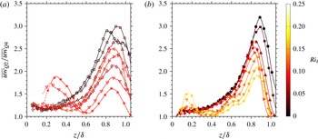
1 Introduction
The atmospheric surface layer is often stably stratified. For example, the nocturnal boundary layer at moderate latitudes can experience significant radiative cooling of the surface, resulting in a stable stratification. Stability can also occur when warm air masses flow (by advection or subsidence) over cold seas or ice, as in polar regions. Our understanding of these flows remains incomplete, and the current models are often insufficient to fully describe their behaviour (Mahrt Reference Mahrt1998, Reference Mahrt2014). Atmospheric measurements within the thermally stable regime are generally difficult since flow unsteadiness increases and flux magnitudes decrease with increasing stability, leading to larger relative errors. Reductions in the integral scale also make turbulence-resolving simulations more challenging (Bou-Zeid et al. Reference Bou-Zeid, Higgins, Huwald, Meneveau and Parlange2010), further reducing the number of tools available for probing the dynamics of stable flows. Laboratory experiments can therefore play an important role. While the Reynolds numbers are typically low compared to the atmosphere, the boundary conditions can be tightly controlled and other influences such as diurnal variations can be excluded. We present extensive laboratory measurements of thermally stratified boundary layers over smooth and rough isothermal walls, and make detailed comparisons with atmospheric data.
The degree of stratification is usually described in terms of a Richardson number. The ratio of the buoyancy flux and turbulent production by mean shear in the turbulent kinetic energy (TKE) equation is called the flux Richardson number,
 $$\begin{eqnarray}Ri_{f}=\frac{g}{T_{0}}\frac{\overline{w\unicode[STIX]{x1D703}}}{\overline{uw}\left(\unicode[STIX]{x2202}U/\unicode[STIX]{x2202}z\right)},\end{eqnarray}$$
where
 $\overline{w\unicode[STIX]{x1D703}}$
is the wall-normal heat flux and
 $\overline{uw}$
is the Reynolds shear stress. Here,
 $z$
is the wall-normal direction,
 $g$
is the acceleration due to gravity and
 $T_{0}$
is a reference temperature, here chosen to be the free stream temperature. Temperature fluctuations are denoted by the variable
 $\unicode[STIX]{x1D703}$
, and velocity fluctuations are indicated by
 $u$
,
 $v$
and
 $w$
, relative to the mean velocities
 $U$
,
 $V$
and
 $W$
in the
 $x$
- (streamwise),
 $y$
- (spanwise) and
 $z$
- (wall-normal) directions, respectively. The overline denotes an ensemble average.
More easily measured, and related to the flux Richardson number through the turbulent Prandtl number
 $Pr_{t}$
, is the gradient Richardson number, defined in terms of the mean gradients of temperature and streamwise velocity so that
 $$\begin{eqnarray}Ri=\frac{g}{T_{0}}\frac{\unicode[STIX]{x2202}T/\unicode[STIX]{x2202}z}{\left(\unicode[STIX]{x2202}U/\unicode[STIX]{x2202}z\right)^{2}}=\frac{N^{2}}{\left(\unicode[STIX]{x2202}U/\unicode[STIX]{x2202}z\right)^{2}}=Pr_{t}\;Ri_{f}.\end{eqnarray}$$
Here,
 $N=\sqrt{(g/T_{0})\unicode[STIX]{x2202}T/\unicode[STIX]{x2202}z}$
is the Brunt–Väisälä frequency (a measure of static stability). The turbulent Prandtl number has conventionally been assumed to be close to unity for neutrally and weakly stratified layers, but it can increase significantly at higher stratification levels (see Zilitinkevich et al.
Reference Zilitinkevich, Elperin, Kleeorin, Rogachevskii and Esau2013; Katul et al.
Reference Katul, Porporato, Shah and Bou-Zeid2014).
In experimental studies, the bulk Richardson number
 $Ri_{\unicode[STIX]{x1D6FF}}$
is often used and defined as
 $$\begin{eqnarray}Ri_{\unicode[STIX]{x1D6FF}}=\frac{g\unicode[STIX]{x1D6FF}}{T_{0}}\frac{\unicode[STIX]{x0394}T}{U_{\infty }^{2}}.\end{eqnarray}$$
Here,
 $\unicode[STIX]{x0394}T$
is the temperature difference across a boundary layer of thickness
 $\unicode[STIX]{x1D6FF}$
. For stable stratification, all Richardson numbers are positive.
A number of laboratory experiments have been performed to complement the studies in the atmosphere (Arya & Plate Reference Arya and Plate1969; Plate & Arya Reference Plate and Arya1969; Nicholl Reference Nicholl1970; Arya Reference Arya1975; Piat & Hopfinger Reference Piat and Hopfinger1981; Ogawa et al.
Reference Ogawa, Diosey, Uehara and Ueda1982, Reference Ogawa, Diosey, Uehara and Ueda1985; Ohya, Neff & Meroney Reference Ohya, Neff and Meroney1997; Ohya Reference Ohya2001; Ohya & Uchida Reference Ohya and Uchida2003, Reference Ohya and Uchida2004; Demarco et al.
Reference Demarco, Puhales, Acevedo, Costa, Avelar and Fisch2015; Puhales et al.
Reference Puhales, Demarco, Martins, Acevedo, Degrazia, Welter, Costa, Fisch and Avelar2015). Of these, the studies by Arya (
 $Ri_{\unicode[STIX]{x1D6FF}}<0.1$
), Ogawa et al. (
 $Ri_{\unicode[STIX]{x1D6FF}}<0.25$
), Ohya et al. (
 $Ri_{\unicode[STIX]{x1D6FF}}<1.33$
), Ohya (
 $Ri_{\unicode[STIX]{x1D6FF}}<1.31$
) and Demarco et al. (
 $Ri_{\unicode[STIX]{x1D6FF}}<0.06$
) allowed the thermal boundary layer to develop over a heated or cooled wall without prescribing a particular temperature profile. Based on this work, it is now well known that turbulence is rapidly suppressed by increasing stratification as energy is extracted from the
 $\overline{w^{2}}$
(direct buoyant destruction) and
 $-\overline{uw}$
(suppression of shear generation) stresses due the additional energy required to overcome buoyancy.
In an important observation, Ohya et al. (Reference Ohya, Neff and Meroney1997) identified the transition between a weakly stable regime and a strongly stable regime (on a smooth wall) as the point where the peak in the turbulent stresses moved far into the outer layer and near-wall turbulence was strongly damped, creating a region of small counter-gradient heat flux. Internal gravity waves and Kelvin–Helmholtz instabilities were also observed at high stratification levels. In Ohya et al. (Reference Ohya, Neff and Meroney1997), and a later rough-wall experiment (Ohya Reference Ohya2001), the two regimes were delineated by a critical bulk Richardson number,
 $Ri_{\unicode[STIX]{x1D6FF},cr}=0.25$
, which Ohya interpreted as being an expected value since it agreed with the classical result of Taylor (Reference Taylor1931) and Miles & Howard (Reference Miles and Howard1964) for the instability of a laminar flow with constant shear.
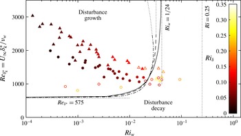
In this respect, Schlichting (Reference Schlichting1935, Reference Schlichting1979) conducted a more complete analysis of the instability of laminar shear flows that accounted for profile curvature, which is necessary to characterize the critical layer and global stability of the boundary layer. His stability curves were expressed in terms of the gradient Richardson number evaluated at the wall, and were Reynolds number and weakly Froude number dependent. A high Reynolds number asymptote of
 $Ri_{w,cr}=1/24$
(
 $=0.042$
) was demonstrated for
 $Fr=0$
. Schlichting’s analysis does not seem to have been widely appreciated, and no detailed comparison with experimental data appears to have been performed until now.
The interpretation of Ohya et al.’s results is further complicated by the fact that their levels of free stream turbulence increased (as a fraction of the free stream velocity) with increasing Richardson number, since the Richardson number was increased by reducing the free stream velocity. As a result, the outer layer turbulence peak they observed in the streamwise and wall-normal directions for strong stratification is comparable in magnitude to their free stream turbulence level of 3 %–4 % of
 $U_{\infty }$
.
The applicability of laboratory results to our understanding of the atmospheric surface layer is also an open question. In laboratory scale experiments with significant stratification, that is, high Richardson number, the Reynolds number is usually small, simply because the Richardson number is proportional to
 $U_{\infty }^{-2}$
and the boundary layer thickness,
 $\unicode[STIX]{x1D6FF}$
. To date, this problem has only been examined by Plate & Arya (Reference Plate and Arya1969) who demonstrated a correspondence between Monin–Obukhov Similarity Theory (MOST) and the experiments of Arya (Reference Arya1968) over a limited range of wall-normal positions
 $(0.01\leqslant z/\unicode[STIX]{x1D6FF}\leqslant 0.15)$
. This dataset was expanded by Arya (Reference Arya1975). The functional forms (logarithmic or power law) and their coefficients, however, were found to be significantly different than those subsequently established for the atmospheric surface layer (Stull Reference Stull1988), suggesting that Reynolds number effects are important. The influence of the Reynolds number was also corroborated by numerical studies and theoretical analyses of Chung & Matheou (Reference Chung and Matheou2012) and Shah & Bou-Zeid (Reference Shah and Bou-Zeid2014). To complicate matters further, Reynolds and Richardson numbers vary simultaneously with increasing stability, so that it is difficult to discriminate between the effects of buoyancy and inertia. Somewhat surprisingly, previous laboratory work has only examined changes in turbulence intensity relative to the free stream velocity. Such a scaling does not remove Reynolds number effects in neutrally stable flows, and therefore is unlikely to isolate the effects due to stratification alone.
Here, we use particle image velocimetry (PIV) and thermocouple rakes to examine a wide range of low Reynolds number, thermally stratified boundary layers with bulk stratifications as strong as
 $Ri_{\unicode[STIX]{x1D6FF}}\approx 0.25$
. Experiments were conducted for both smooth and rough walls to improve correspondence with the atmospheric surface layer, where the wall is almost always fully rough. Coriolis forces were not considered. Despite the Ekman turning of the mean flow induced by Coriolis forces, such forces have been shown to cause little effect on turbulent statistics for weak to moderate stability in atmospheric measurements (Grachev et al.
Reference Grachev, Fairall, Persson, Andreas and Guest2005), and although they grow in influence as the fluxes reduce for stronger levels of stability, it then becomes difficult to discriminate between stratification and Coriolis effects. As such, the absence of this force in the current experiments can be considered an asset.
In an effort to isolate the effects of Reynolds number, we use inner and outer similarity variables commonly used when scaling wall-bounded turbulent flows. For the inner and outer regions of the layer the velocity scale is the friction velocity
 $u_{\unicode[STIX]{x1D70F}}=\sqrt{\unicode[STIX]{x1D70F}_{w}/\unicode[STIX]{x1D70C}_{w}}$
, where
 $\unicode[STIX]{x1D70F}_{w}$
is the wall stress and
 $\unicode[STIX]{x1D70C}_{w}$
is the fluid density at the wall. For the inner part, the length scale is
 $\unicode[STIX]{x1D708}_{w}/u_{\unicode[STIX]{x1D70F}}$
, where
 $\unicode[STIX]{x1D708}_{w}$
is the kinematic viscosity at the wall, and for the outer part the length scale is
 $\unicode[STIX]{x1D6FF}$
. We find good correspondence over much of the boundary layer between our low Reynolds number laboratory experiments and atmospheric data in the gradient-based atmospheric scaling of Sorbjan (Reference Sorbjan2010), which suggests that our results are broadly applicable across all Reynolds numbers. In particular, we propose that the weak/strong criterion suggested by Ohya et al. (Reference Ohya, Neff and Meroney1997) needs to be modified.
2 Experimental details
The experiments were conducted in Princeton Gas Dynamics Laboratory’s low-speed wind tunnel. The tunnel is open-return and is 5 m long with a
 $1.2\times 0.9~\text{m}^{2}$
cross-section and a maximum free stream velocity of
 $U_{\infty }=2.4~\text{m}~\text{s}^{-1}$
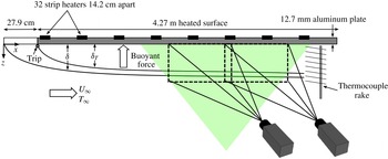
. In previous laboratory studies of stratified boundary layers, heated air was passed over a cooled bottom surface. In our experiment, air enters the tunnel at room temperature before passing under a strongly heated upper surface, as shown in figure 1, creating a stable buoyancy force that acts upwards toward the surface. The upper surface is a 12.7 mm-thick sheet of aluminium that can be isothermally heated along its entire length to a maximum temperature of
 $135\pm 2\,^{\circ }\text{C}$
using a set of 32 resistive heating strips. A nominally zero pressure gradient turbulent boundary layer develops over the upper surface, tripped using a 6.35 mm (1/4”) rod located at the leading edge of the heated plate. The measurement region was located a distance of 3.75 m downstream of the trip.
Note that for a heated surface, the density and viscosity decrease with distance from the wall, whereas with a cooled surface the trend is reversed. The high wall temperatures employed in our study cause the density and viscosity to vary by up to 30 % from the wall to free stream, so that the kinematic viscosity can be up to 80 % larger at the wall than that in the free stream. These fluid property variations need to be taken into account, particularly when assessing Reynolds number effects, as we will show. Dilatation effects may also be important, and it will be examined how such effects can be accounted for in the scaling.
A schematic of the experimental set-up.

Tests were conducted using both smooth and rough surfaces. For the rough surface, a woven wire mesh of thickness
 $k=4.1$
mm was used, similar to that studied by Flack, Schultz & Shapiro (Reference Flack, Schultz and Shapiro2005) and Flack, Schultz & Connelly (Reference Flack, Schultz and Connelly2007). The wire mesh was a square weave with a wire size of 2.05 mm and a pitch of 12.7 mm, oriented with the wires running in the streamwise and spanwise directions. All PIV data were acquired in a streamwise-vertical plane located between two streamwise wires. For the neutrally stratified cases, the roughness height corresponds to
 $\unicode[STIX]{x1D6FF}/k=30{-}31$
and
 $k^{+}=11{-}39$
, where the superscript
 $+$
denotes normalization using the friction velocity scale
 $u_{\unicode[STIX]{x1D70F}}$
and the inner length scale
 $\unicode[STIX]{x1D708}_{w}/u_{\unicode[STIX]{x1D70F}}$
.
Roughness causes a downward shift in the logarithmic portion of the mean velocity profile by an amount called the roughness function,
 $\unicode[STIX]{x0394}U^{+}$
. Nikuradse (Reference Nikuradse1933) proposed that different roughness geometries could be compared by defining a roughness length scale
 $k_{s}$
, called the equivalent sand grain roughness, defined in terms of the roughness function so that
 $$\begin{eqnarray}\unicode[STIX]{x0394}U^{+}=\frac{1}{\unicode[STIX]{x1D705}}\ln (k_{s}^{+})+B-8.5.\end{eqnarray}$$
We found
 $k_{s}^{+}=44{-}124$
for the neutrally stratified boundary layer cases reported here. In (2.1),
 $\unicode[STIX]{x1D705}$
and
 $B$
are, respectively, the von Kármán constant and the additive constant in the logarithmic law for the mean velocity profile. The values were taken to be
 $\unicode[STIX]{x1D705}=0.421$
and
 $B=5.6$
(McKeon et al.
Reference McKeon, Li, Jiang, Morrison and Smits2004), but our conclusions are not sensitive to the choice of log-law constants. Note that the roughness length
 $z_{0}$
, scaled using inner variables, is given by
 $z_{0}^{+}=\exp [\unicode[STIX]{x1D705}(\unicode[STIX]{x0394}U^{+}-B)]=1.23{-}3.39$
.
The values of
 $\unicode[STIX]{x1D6FF}/k$
and
 $k^{+}$
are close to those found in other studies using woven wire mesh where outer similarity was observed (Connelly, Schultz & Flack Reference Connelly, Schultz and Flack2006; Flack et al.
Reference Flack, Schultz and Connelly2007), indicating that the effects of roughness are confined to a roughness sublayer near the wall in line with Townsend’s wall-similarity hypothesis (Townsend Reference Townsend1976). Such flows are termed fully rough (Jimenez Reference Jimenez2004).
Large field-of-view, two dimensional, two-component velocity measurements were obtained in the (
 $x$
–
 $z$
)-plane using PIV. The large field-of-view was created by partially overlapping two 5.5 megapixel sCMOS camera images in the streamwise direction (see figure 1). The resulting vector fields could then be merged into a
 $160\times 300$
mm
 $^{2}$
domain, which corresponded to approximately
 $1.25\unicode[STIX]{x1D6FF}\times 2.3\unicode[STIX]{x1D6FF}$
for neutral conditions.
Light was provided by a 50 mJ dual-pulse Nd:YAG laser in conjunction with a Powell lens to create the light sheet and a focal lens to narrow the sheet thickness in the measurement domain (
 ${\sim}1$
mm). The flow was seeded using 1
 $\unicode[STIX]{x03BC}$
m mineral oil smoke particles generated by a MAX 3000 MDG fog generator.
Velocity fields were computed using a multi-grid, multi-pass cross-correlation method with iterative image deformation (Huang, Fiedler & Wang Reference Huang, Fiedler and Wang1993; Jambunathan et al.
Reference Jambunathan, Ju, Dobbins and Ashforth-Frost1995; Nogueira, Lecuona & Rodriguez Reference Nogueira, Lecuona and Rodriguez1999; Scarano Reference Scarano2002) as implemented in DaVis 8.1.6. The two camera frames were merged using functions internal to DaVis. The window size of the final pass was
 $32\times 32$
pixels with a 50 % overlap, resulting in a grid spacing of
 $\unicode[STIX]{x0394}x^{+}=\unicode[STIX]{x0394}z^{+}=3{-}12$
for the neutrally stratified smooth and rough-wall cases. The friction velocity was found to decrease substantially with stable thermal stratification, improving the grid spacing to values as low as
 $\unicode[STIX]{x0394}x^{+}=\unicode[STIX]{x0394}z^{+}=1.5$
.
Due to drop outs in near-wall seeding at the highest wall temperatures, special care was taken to remove spurious vectors. This was initially accomplished by removing all vectors with a peak ratio of less than 1.1, in conjunction with a normalized median filter (Westerweel & Scarano Reference Westerweel and Scarano2005) greater than two standard deviations of a
 $5\times 5$
neighbourhood. No filtered vectors or alternate correlation peaks were reinserted at this stage. Under neutral conditions the valid-vector yield was 99 %. With increasing wall temperature, an increasing number of near-wall vectors were determined to be invalid, and so we mark the wall distance below which at least 10 % of vectors were missing as
 $z_{10\,\%}$
.
A small number of vectors were reinserted from alternate correlation peaks, satisfying a normalized local median filter of three standard deviations. This had the effect of filling a small number of data holes while having a negligible impact on vector statistics above
 $z_{10\,\%}$
. It also had the effect of slightly increasing data yield towards the wall, but since these vectors were derived from small peak ratios, any data presented below
 $z_{10\,\%}$
are shown using dotted lines.
Finally, a narrow-band Gaussian spatial filter was employed to remove noise associated with frequencies larger than the sampling frequency of the interrogation, as is now common practice (Adrian, Meinhart & Tomkins Reference Adrian, Meinhart and Tomkins2000; Wu & Christensen Reference Wu and Christensen2006). For all flow speeds and wall temperatures, 750 image pairs were acquired at a rate of 15 Hz.
Bias errors due to peak locking were limited by ensuring particle image sizes were greater than two pixels. Under these conditions the random error was dominated by noise in particle image recording, which accounted for approximately 5 % of the particle image diameter or approximately 0.1 pixels, as shown by Prasad et al. (Reference Prasad, Adrian, Landreth and Offutt1992). Interframe times were selected to maintain a free stream particle displacement of approximately 8 pixels and thus random errors in velocity were estimated to be approximately 1.25 % of the free stream velocity. Other errors due to convergence of statistics and merging of velocity fields yielded total uncertainties for
 $\overline{u^{2}}$
,
 $\overline{w^{2}}$
and
 $\overline{uw}$
of
 $\pm 3\,\%$
,
 $\pm 5\,\%$
and
 $\pm 7\,\%$
, respectively, at the lowest free stream velocity, and reduce with increasing free stream velocity. These values were estimated by comparing statistical profiles based on results from each PIV camera in isolation as well as those based on half the total number of PIV images.
A thermocouple rake was used to obtain the mean temperature profile. The rake consisted of 14 fine-wire thermocouples covering a maximum wall-normal distance of 128.6 mm and with a minimum thermocouple spacing of 4.76 mm near the wall. This spacing was doubled and then quadrupled with increasing distance from the wall. The rake was offset from the PIV laser sheet by 5 mm in the spanwise direction and placed just outside the field of view in the downstream direction. The wall-normal position of the thermocouple closest to the wall was measured using calibrated macro-photography. All thermocouples were monitored in sets of seven using a National Instruments PCI-6229 board, accurate to
 $\pm 1\,^{\circ }\text{C}$
. Cold junction compensation of the set of seven thermocouples closest to the wall was done separately to those further from the wall, resulting in a small bias error between each set that might affect estimates of the mean temperature gradient. A small correction
 $({<}1\,^{\circ }\text{C})$
was applied by symmetrically shifting each group of temperature measurements such that the temperature gradient at the location between them was equal to the average of the gradients estimated on either side (using a linear fit to the two closest thermocouples). Also, a cubic interpolation was used to extrapolate the temperature profile to the free stream for those few cases where the boundary layer was thicker than the full rake height.
The heating power input was limited to 4.1 kW, and so to obtain the highest velocity/temperature cases, the plate was allowed to reach thermal equilibrium at low speed, before increasing the velocity for the brief period during which data were acquired, taking advantage of the high thermal mass of the thick aluminium plate to keep the boundary condition approximately constant. Using this approach, the maximum drop in wall temperature during a run was
 $2\,^{\circ }\text{C}$
, with the greatest drop near the leading edge, and the rake thermocouple nearest to the wall was seen to be stable to within
 $1.5\,^{\circ }\text{C}$
or 4.5 % of the wall–free stream temperature difference, whichever was more strict for a given case. For the rough-wall data, the near-wall flow temperature was stable to within
 $1.5\,^{\circ }\text{C}$
or 3.5 %.
3 Flow conditions
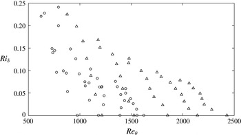
Experimental parameter space for all wall temperatures and free stream velocities: ○ smooth; ▵ rough.

To achieve a wide range of Reynolds and Richardson numbers, five free stream velocities were investigated, from
 $U_{\infty }=1.2$
to
 $2.4~\text{m}~\text{s}^{-1}$
, and for each velocity, eight isothermal wall temperatures were studied, from room temperature (approximately
 $26\,^{\circ }\text{C}$
) to
 $T_{w}=135\,^{\circ }\text{C}$
. The resulting range of Reynolds number and Richardson number combinations are shown in figure 2. Here,
 $Re_{\unicode[STIX]{x1D703}}=U_{\infty }\unicode[STIX]{x1D703}/\unicode[STIX]{x1D708}_{\infty }$
is the momentum thickness Reynolds number, where
 $\unicode[STIX]{x1D708}_{\infty }$
is the kinematic viscosity evaluated at the free stream temperature. The displacement and momentum thicknesses for variable density flows (
 $\unicode[STIX]{x1D6FF}^{\ast }$
and
 $\unicode[STIX]{x1D703}$
, respectively) are defined in the usual way as
 $$\begin{eqnarray}\unicode[STIX]{x1D6FF}^{\ast }=\int _{0}^{\infty }\left(1-\frac{\unicode[STIX]{x1D70C}U}{\unicode[STIX]{x1D70C}_{\infty }U_{\infty }}\right)\,\text{d}z\quad \text{and}\quad \unicode[STIX]{x1D703}=\int _{0}^{\infty }\frac{\unicode[STIX]{x1D70C}U}{\unicode[STIX]{x1D70C}_{\infty }U_{\infty }}\left(1-\frac{U}{U_{\infty }}\right)\,\text{d}z.\end{eqnarray}$$
The mean density was computed from the temperature profile (since the pressure may be assumed constant), and the integrals were evaluated only up to the boundary layer thickness,
 $\unicode[STIX]{x1D6FF}$
. The temperature was assumed to vary linearly for the short distance from the edge of the thermocouple rake to
 $T_{\infty }$
at
 $\unicode[STIX]{x1D6FF}$
for those cases where the boundary layer was larger than the thermocouple rake. Here, we define the boundary layer thickness
 $\unicode[STIX]{x1D6FF}$
as the distance from the wall where the mean streamwise velocity is equal to its maximum value because we found a small overshoot in velocity near the edge of the boundary layer for the current experiments. The thickness according to this definition is 12 %–20 % larger than
 $\unicode[STIX]{x1D6FF}_{99}$
, the distance from the wall at which the velocity reaches 99 % of the free stream velocity. The momentum and displacement thickness values are estimated to be accurate to 2 %.
For neutral stratification (
 $\unicode[STIX]{x0394}T=0$
), the Reynolds number range was
 $970\leqslant Re_{\unicode[STIX]{x1D703}}\leqslant 1600$
(smooth wall) and
 $1200\leqslant Re_{\unicode[STIX]{x1D703}}\leqslant 2400$
(rough wall). For the highest temperature and lowest velocity conditions, the bulk Richardson numbers approach 0.25 over both smooth and rough surfaces. From figure 2, we see that the Reynolds number decreases as the stratification level increases. At the same time, the boundary layer thickness decreases due to reduced mixing, and so, for a given velocity, the Richardson number does not increase linearly with the wall temperature.
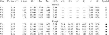
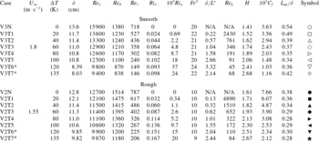
The flow conditions for the neutral stability cases are summarized in table 1, and the flow conditions for stably stratified cases at two particular velocities are given in table 2. We choose to highlight Case V3
 $(U_{\infty }=1.8~\text{m}~\text{s}^{-1})$
for the smooth wall, and V2
 $(U_{\infty }=1.55~\text{m}~\text{s}^{-1})$
for the rough wall. Results at other velocities show similar trends.
In tables 1 and 2,
 $Re_{\unicode[STIX]{x1D70F}}=u_{\unicode[STIX]{x1D70F}}\unicode[STIX]{x1D6FF}/\unicode[STIX]{x1D708}_{w}$
,
 $Re_{\unicode[STIX]{x1D6FF}}=U_{\infty }\unicode[STIX]{x1D6FF}/\unicode[STIX]{x1D708}_{\infty }$
,
 $C_{f}=2\unicode[STIX]{x1D70F}_{w}/(\unicode[STIX]{x1D70C}_{\infty }U_{\infty }^{2})$
is the skin friction coefficient,
 $H=\unicode[STIX]{x1D6FF}^{\ast }/\unicode[STIX]{x1D703}$
is the boundary layer shape factor, and
 $L_{uu}$
is the integral scale of the streamwise velocity fluctuations. The subscripts indicate the reference conditions for the fluid properties;
 $w$
corresponds to wall conditions, and
 $\infty$
corresponds to free stream conditions. Also,
 $\unicode[STIX]{x1D6F1}$
is Coles’s wake factor, where
 $\unicode[STIX]{x1D6F1}=\unicode[STIX]{x1D705}\unicode[STIX]{x1D6E5}_{0}/2$
and
 $\unicode[STIX]{x1D6E5}_{0}$
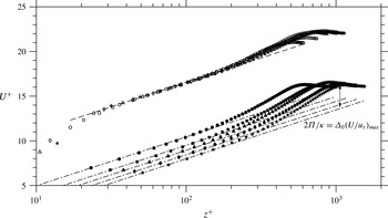
is the maximum distance between the inner scaled mean velocity profile and the log law in the outer portion of the boundary layer (see figure 3 for illustration). The Froude number,
 $Fr=U_{\infty }/\sqrt{g\unicode[STIX]{x1D6FF}_{k}^{\ast }}$
, is defined in terms of the kinematic version of the displacement thickness,
 $$\begin{eqnarray}\unicode[STIX]{x1D6FF}_{k}^{\ast }=\int _{0}^{\infty }\left(1-\frac{U}{U_{\infty }}\right)\,\text{d}z,\end{eqnarray}$$
which ignores changes in fluid density and is identical to that used in incompressible and isothermal flows. The Monin–Obukhov length
 $L^{\ast }=-u_{\unicode[STIX]{x1D70F}}^{3}/\left(\unicode[STIX]{x1D705}g/T_{\infty }Q_{w}\right)$
, where
 $Q_{w}=\unicode[STIX]{x1D6FC}_{w}\unicode[STIX]{x2202}T/\unicode[STIX]{x2202}z|_{z=0}$
and
 $\unicode[STIX]{x1D6FC}_{w}$
is the thermal diffusivity of the fluid at the wall temperature. The temperature gradient at the wall is estimated using data from near-wall thermocouples (see § 5.2). The Reynolds number,
 $Re_{L}=L^{\ast }u_{\unicode[STIX]{x1D70F}}/\unicode[STIX]{x1D708}_{w}$
is discussed in § 6. The gradient Richardson number evaluated at the wall (
 $Ri_{w}$
) is estimated as described in § 6.1.
Flow conditions for neutral boundary layer tests.

Flow conditions for stably stratified boundary layer tests. Only the cases for
 $U_{\infty }=1.8~\text{m}~\text{s}^{-1}$
(smooth) and
 $U_{\infty }=1.55~\text{m}~\text{s}^{-1}$
(rough) are listed. An asterisk next to a case name indicates that it was subsequently found to be in the collapsed regime, where turbulent velocity statistics no longer scale with the wall shear stress.

4 Neutral boundary layer
We now examine the effects of Reynolds number and roughness on neutral boundary layer statistics so that the effects of stratification in the stable boundary layer experiments can be more clearly identified.
The mean velocity profiles for the smooth- and rough-wall neutral boundary layers are shown in figure 3. The smooth-wall cases appear as expected, with a constant wake factor of about 0.2, typical of a zero pressure gradient flow at low Reynolds numbers. The rough-wall boundary layers appear to follow the wall-similarity hypothesis of Townsend (Reference Townsend1976), in that the effect of surface roughness is confined to the inner layer, causing a downward shift of the logarithmic profile by a distance
 $\unicode[STIX]{x0394}U^{+}$
(the roughness function), as identified by Clauser (Reference Clauser1954) and Hama (Reference Hama1954). The wake strength
 $\unicode[STIX]{x1D6F1}$
in the rough-wall case is somewhat larger than that seen in the smooth-wall case, which may be partly due to the increase in Reynolds number.
For the smooth-wall cases shown in figure 3, the Clauser chart method (Clauser Reference Clauser1954) was used to determine the friction velocity
 $u_{\unicode[STIX]{x1D70F}}$
. For the rough-wall cases, the modified Clauser chart method originated by Perry, Schofield & Joubert (Reference Perry, Schofield and Joubert1969) was used. Because the true position of the wall is unknown when roughness is present, three parameters were fitted: the roughness function, friction velocity and virtual origin (referred to in the geophysical literature as the displacement height).
Neutral boundary layer mean velocity profiles in inner coordinates at free stream velocities from
 $U_{\infty }=0.96$
to
 $2.63~\text{m}~\text{s}^{-1}$
. Symbols according to table 1. Every other data point shown for clarity. – – – Log law with
 $\unicode[STIX]{x1D705}=0.421$
and
 $B=5.6$
. – - – - – Rough-wall log-law profiles, where the intercept is less than the smooth-wall value by an amount equal to the roughness function,
 $\unicode[STIX]{x0394}U^{+}$
.

The friction velocity can also be estimated using the maximum total shear stress near the wall, given by the sum of the turbulent and viscous stresses,
 $$\begin{eqnarray}\unicode[STIX]{x1D70F}_{w}=\unicode[STIX]{x1D70C}_{w}u_{\unicode[STIX]{x1D70F}}^{2}\approx \left(\frac{\unicode[STIX]{x2202}}{\unicode[STIX]{x2202}z}\left(\unicode[STIX]{x1D707}U\right)-\unicode[STIX]{x1D70C}\overline{uw}\right)_{wall},\end{eqnarray}$$
which for an incompressible/isothermal flow reduces to
 $$\begin{eqnarray}u_{\unicode[STIX]{x1D70F}}\approx \left(\unicode[STIX]{x1D708}\frac{\unicode[STIX]{x2202}U}{\unicode[STIX]{x2202}z}-\overline{uw}\right)_{wall}^{1/2}.\end{eqnarray}$$
The total stress was measured at the closest point to the wall where the PIV cross-correlation windows did not overlap with the wall image. Equation (4.1) was used for all stratified cases while (4.2) was only employed for neutral conditions.
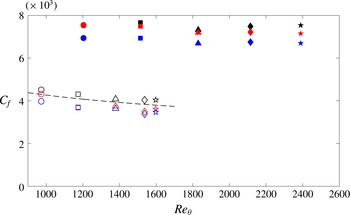
For the Reynolds numbers in this study, the viscous portion of the total shear stress extends for a significant fraction of the boundary layer, and so the peak in the turbulent shear stress profile does not attain the same value as the wall shear stress. A correction can be applied using the second-order asymptotic analysis of Panton (Reference Panton1990) which provides an improved estimate of the friction velocity. The estimated skin-friction coefficients are compared in figure 4. Overall, the different friction velocity estimates vary by
 $\pm 4.5$
% and
 $\pm 3$
% for the smooth and rough neutral cases, respectively. Friction values estimated from the total stress are consistently slightly lower than those from the Clauser chart method.
Neutral boundary layer skin-friction variation with Reynolds number. Symbols as in table 1. Open symbols refer to smooth-wall cases and filled symbols refer to rough-wall cases. Black: Clauser chart method. Blue: total stress method. Red: matching the peak turbulent shear stress to the estimate of Panton (Reference Panton1990). The low Reynolds number correlation of Smits, Matheson & Joubert (Reference Smits, Matheson and Joubert1983) is shown as a dashed line.

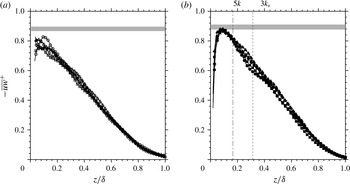
The turbulent shear stress is seen to scale well when employing outer variables, as indicated in figure 5 where
 $-\overline{uw}^{+}=-\overline{uw}/u_{\unicode[STIX]{x1D70F}}^{2}$
. A shaded region indicates the range over which the peak turbulent shear stress varies for this Reynolds number interval according to Panton (Reference Panton1990). As expected, the peak values do not obtain a value of unity due to the low Reynolds number. The peak smooth-wall values are somewhat lower than the Panton estimate but still within the error estimates given here and in § 2. The small scatter in the rough-wall data is also within experimental error and does not seem to correlate with
 $k^{+}$
. The vertical lines in figure 5(b) indicate the maximum extent of the roughness sublayer for the highest Reynolds number case, based on estimates of
 $5k$
and
 $3k_{s}$
given by Flack et al. (Reference Flack, Schultz and Connelly2007). Note that the
 $3k_{s}$
estimate encompasses approximately 30 % of the boundary layer thickness.
Neutral boundary layer profiles of turbulent shear stress, in outer coordinates (
 $-\overline{uw}^{+}=-\overline{uw}/u_{\unicode[STIX]{x1D70F}}^{2}$
). Symbols as in table 1. Friction velocity as determined from Clauser chart method. – - – - –,
 $5k$
; - - - -,
 $3k_{s}$
(shown for the highest Reynolds number case only). Shaded region indicates the range over which the peak turbulent shear stress varies for this Reynolds number interval according to Panton (Reference Panton1990). Every other data point is shown for clarity. (a) Smooth, (b) rough.

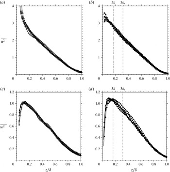
The streamwise (
 $\overline{u^{2}}^{+}=\overline{u^{2}}/u_{\unicode[STIX]{x1D70F}}^{2}$
) and wall-normal (
 $\overline{w^{2}}^{+}=\overline{w^{2}}/u_{\unicode[STIX]{x1D70F}}^{2}$
) stresses for the smooth and rough walls are shown in figure 6. For both components, the smooth-wall profiles show excellent scaling in outer variables, well within experimental error. The results for the rough wall scale almost as well, and show the expected behaviour near the wall for fully rough flows (Ligrani & Moffat Reference Ligrani and Moffat1986). The effects of roughness appear to be confined to a region
 $z\leqslant 3k$
.
Neutral boundary layer profiles of streamwise and wall-normal variance. Symbols as in table 1. Wall-normal distances of
 $5k$
and
 $3k_{s}$
are indicated for the highest Reynolds number case only. (a) Smooth – streamwise variance, (b) rough – streamwise variance, (c) smooth – wall-normal variance, (d) rough – wall-normal variance.

5 Stably stratified boundary layer
We now examine the effects of thermal stratification. As indicated earlier, we highlight two specific cases: Case V3
 $(U_{\infty }=1.8~\text{m}~\text{s}^{-1})$
for the smooth wall, and Case V2
 $(U_{\infty }=1.55~\text{m}~\text{s}^{-1})$
for the rough wall (see table 2).
5.1 Mean flow with stratification
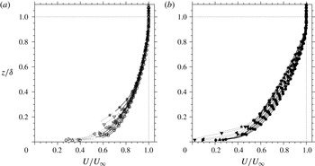
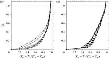
The mean velocity and temperature profiles for these cases are shown in figures 7 and 8. Dotted lines have been used to indicate data below the level at which 10 % of vectors are missing due to insufficient seeding (
 $z_{10\,\%}$
). Alternate vectors, corresponding to correlation peaks that satisfy the median filter, were reinserted into the data to help identify trends below this level but the data in this region must be treated with caution due the low peak ratios of many vectors.
The mean velocity and temperature layers are seen to have very similar thickness and display a strong reduction in wall shear and heat flux as the level of stability increases and the mixing decreases. Mean velocity profiles from the strongest stability cases resemble a laminar profile, and their shape factor,
 $H=\unicode[STIX]{x1D6FF}^{\ast }/\unicode[STIX]{x1D703}$
, tends toward the laminar Blasius value of 2.59. Interestingly, the rough-wall profiles are affected by stratification throughout the entire layer, whereas the smooth-wall profiles are affected only progressively from the wall and agree well for
 $z/\unicode[STIX]{x1D6FF}>0.45$
. It will be shown that this observation helps to explain the differences seen between smooth and rough-wall velocity statistics.
Stable boundary layer mean velocity profiles: (a) smooth wall (case V3); (b) rough wall (case V2), with varying wall temperature. Conditions and symbols as in table 2. Symbols not shown for every wall-normal location, for clarity.

Stable boundary layer mean temperature profiles: (a) smooth wall (case V3); (b) rough wall (case V2), with varying wall temperature. Conditions and symbols as in table 2.

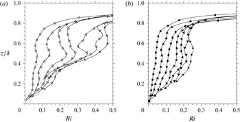
Gradient Richardson number profiles for (a) smooth and (b) rough wall cases. Conditions and symbols as in table 2. Uncertainty increases significantly above
 $z/\unicode[STIX]{x1D6FF}=0.7$
as mean gradients become small.

Profiles of gradient Richardson number are shown in figure 9. Temperature gradients were calculated by differentiating an exponential fit to a moving stencil of three points and then interpolating to the wall-normal locations of the mean velocity profile. Mean velocity gradients employed a nine-point stencil. This method was preferred to a central differencing scheme, which was found to be highly sensitive to the limited number of wall-normal temperature measurements. The remaining waviness in the profile is attributed to the limited number of wall-normal temperature measurements and is not thought to be physical.
We see that the gradient Richardson number profiles for the smooth-wall cases have a small but marked increase near
 $z/\unicode[STIX]{x1D6FF}=0.45$
when moving away from the wall. This was the location above which the mean velocity profile was not significantly affected by stratification. The same local increase is not found in the rough-wall profiles. The bulk Richardson number for the rough-wall cases is larger than for the smooth-wall cases on average, but the gradient Richardson number, indicating local stratification, is smaller in the outer layer than for the smooth-wall cases. This observation underscores the difficulty of identifying the appropriate measure of stability in such stably stratified flows. Differences among the gradient Richardson number profiles for the four highest bulk Richardson numbers are small, but the mean profiles were seen to change sharply. This sensitivity is in accord with the large-eddy simulations of stable boundary layers by Huang & Bou-Zeid (Reference Huang and Bou-Zeid2013) that also indicate a continuous increase in the gradient Richardson number with increasing bulk temperature differences.
The mean velocity and temperature profiles most closely follow those of Arya (Reference Arya1975) and Ogawa et al. (Reference Ogawa, Diosey, Uehara and Ueda1985), who examined smooth-wall turbulent boundary layers developing over an isothermal plate with a uniform inflow temperature. Although these authors did not publish gradient Richardson number profiles, mean velocity and temperature profiles of similar thickness were seen to reduce in fullness with increasing stratification, in turn reducing wall shear, as seen here.
In contrast, the more recent works by Ohya et al. (Reference Ohya, Neff and Meroney1997) and Ohya (Reference Ohya2001) report results that are significantly different to those seen here, despite using experimental set-ups similar to those used by Arya (Reference Arya1975) and Ogawa et al. (Reference Ogawa, Diosey, Uehara and Ueda1985). For a smooth surface, Ohya et al. (Reference Ohya, Neff and Meroney1997) observed little change in the mean temperature profile with increasing stratification, resulting in a maximum in gradient Richardson number near
 $z/\unicode[STIX]{x1D6FF}=0.15$
for increasing bulk stratification. For a rough surface, Ohya (Reference Ohya2001) also observed little change in the shape of the mean temperature profile with increasing stratification. For stronger stratification, an inflection was observed in the mean velocity profiles near the edge of the boundary layer resulting in a maximum in the gradient Richardson number in the outer layer. Such differences in the mean profiles are important because Ohya et al. (Reference Ohya, Neff and Meroney1997) proposed that the peak in near-wall stratification led to the preferential damping of near-wall turbulence, and thereby signified the onset of a new ‘strongly stable’ regime for higher Richardson numbers. Our results do not support the generality of that hypothesis.
Furthermore, Arya (Reference Arya1975) and Ohya et al. (Reference Ohya, Neff and Meroney1997) used the same wind tunnel facility. To obtain a wider range of stably stratified conditions, the later study operated at lower free stream velocities and thus correspondingly lower Reynolds numbers. However, the Reynolds number does not seem to be the issue because the current results compare well with the much higher Reynolds number experiments of Arya (Reference Arya1975), as well as the relatively lower Reynolds number experiments of Ogawa et al. (Reference Ogawa, Diosey, Uehara and Ueda1985). More likely, the differences seen in the mean Richardson number profiles may be due to the different development lengths used upstream and downstream of the cold wall section, as well as the effects of fences and other tripping devices. In addition, the widely spaced chain roughness employed by Ohya (Reference Ohya2001) is akin to the anomalous
 $d$
-type roughness (Jimenez Reference Jimenez2004), potentially further influencing the results. Finally, the high levels of free stream turbulence (up to 4 % of the free stream velocity) experienced in the experiments by Ohya et al. (Reference Ohya, Neff and Meroney1997) and Ohya (Reference Ohya2001) may also have been a factor.
5.2 Monin–Obukhov length estimates
To determine the Monin–Obukhov length, the wall heat flux was estimated by calculating the gradient of the mean temperature profile near the wall using an exponential fit to the three thermocouple measurements closest to the surface, although this method is likely to underestimate the heat flux. The second thermocouple from the wall was always located at
 $y^{+}<44$
.
The results are summarized in table 2. The bulk stability parameter
 $\unicode[STIX]{x1D6FF}/L^{\ast }$
represents the largest possible value of the stability parameter
 $z/L^{\ast }$
. We see that
 $\unicode[STIX]{x1D6FF}/L^{\ast }$
increases with mean temperature difference up to value of approximately 2.5. This is consistent with a region of validity for MOST that shrinks with increasing bulk stratification, as discussed extensively in Mahrt (Reference Mahrt1998). Beyond making this observation, we were not able to evaluate MOST stability functions because the experimental boundary layers do not have a significant constant flux layer and the turbulent heat flux, required to evaluate the local flux-based formulation, was not measured.
5.3 Inner scaling of mean velocity profiles
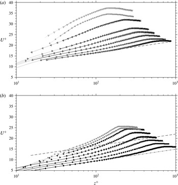
The mean velocity profiles are shown in inner scaling in figure 10, where it was assumed that the virtual origin for the rough wall (one of the three parameters required for scaling rough-wall mean velocity profiles – see § 4) is the same as that found for the neutrally stratified case at the same velocity. Note that the inner length scale,
 $\unicode[STIX]{x1D708}_{w}/u_{\unicode[STIX]{x1D70F}}$
, does not vary across the layer. The friction velocity for stably stratified cases was determined from the near-wall asymptote of the total shear stress as given by (4.1) (the slope of the log law is not known for stable flows and so the Clauser chart method cannot be used). For the smooth- and rough-wall velocities highlighted here, the friction velocity calculated using (4.1) is estimated to be accurate to
 $\pm 10\,\%$
for cases with
 $\unicode[STIX]{x0394}T<100\,^{\circ }\text{C}$
. For the cases with the two highest wall temperatures, the friction velocity estimates are conservatively accurate to only
 $\pm 40\,\%$
and
 $\pm 20\,\%$
for smooth and rough walls respectively, mainly because the near-wall viscous stress is a greater proportion of the total stress, and the location where 10 % of vectors were missing (
 $z_{10\,\%}$
) was further from the wall than the maximum turbulent shear stress as a result of deterioration in near-wall seeding quality (relatively better seeding remained near the rough wall). Grey symbols are used for these cases to acknowledge these higher levels of uncertainty, although we will show that such uncertainties will not affect our basic conclusions.
Stable boundary layer mean velocity profiles in inner scaling for (a) smooth and (b) rough walls. Profiles shown in grey correspond to those datasets where the estimate of
 $u_{\unicode[STIX]{x1D70F}}$
has greater uncertainty due to reductions in near-wall seeding quality. Conditions and symbols as in table 2. Every other data point shown for clarity. – – – Log law with
 $\unicode[STIX]{x1D705}=0.421$
and
 $B=5.6$
. – - – - – Log law shifted downward by the roughness function,
 $\unicode[STIX]{x0394}U^{+}$
, for neutral case.

Weak stratification causes an upward shift in the log-region intercept, consistent with a thickening of the viscous sublayer. As the level of stratification increases, the profiles increase in slope and tend toward a more laminar shape. The smooth- and rough-wall cases follow the same trend, with a greater change for those with a smooth wall. The results are consistent with those of Arya (Reference Arya1975), which is the only other experimental study to examine the effect of stable stratification on mean velocity profiles in this scaling.
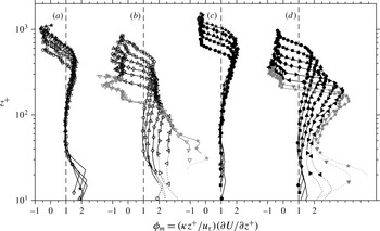
The increasing slope of the mean velocity profile can be highlighted by examining the non-dimensional velocity gradient,
 $$\begin{eqnarray}\unicode[STIX]{x1D719}_{m}=\frac{\unicode[STIX]{x1D705}z^{+}}{u_{\unicode[STIX]{x1D70F}}}\frac{\unicode[STIX]{x2202}U}{\unicode[STIX]{x2202}z^{+}},\end{eqnarray}$$
which is plotted in inner coordinates in figure 11. The neutral boundary layer cases are included for comparison. Under the effect of stratification, the smooth-wall velocity profiles are seen to increase in slope by as much as a factor of 5, while the rough-wall cases increase only by a factor of 2.5 (discounting data below
 $z_{10\,\%}$
, indicated with dotted lines).

More broadly speaking, the mean velocity gradient profiles invite a similarity analysis. To take into account the variations in fluid properties across the layer, we look to the van Driest transformation (van Driest Reference van Driest1951, Reference van Driest1956) for guidance. This transformation successfully scales compressible mean velocity profiles onto the conventional log law (see Smits & Dussage Reference Smits and Dussage2005). van Driest proposed that the correct friction velocity should be based on the local shear stress, which deviates from its wall value due to changes in fluid density. That is, we use a local velocity scale
 $u_{\ast }=\sqrt{\unicode[STIX]{x1D70F}_{w}/\unicode[STIX]{x1D70C}}$
. It will be subsequently demonstrated that the turbulence profiles of the current stably stratified dataset show an improved collapse when scaling with
 $u_{\ast }$
. In gradient form, the van Driest transformation suggests a similarity variable
 $$\begin{eqnarray}\unicode[STIX]{x1D719}_{m}^{\ast }=\sqrt{\frac{\unicode[STIX]{x1D70C}}{\unicode[STIX]{x1D70C}_{w}}}\frac{\unicode[STIX]{x1D705}z^{+}}{u_{\unicode[STIX]{x1D70F}}}\frac{\unicode[STIX]{x2202}U}{\unicode[STIX]{x2202}z^{+}}.\end{eqnarray}$$
However, the effect of stable stratification is always to increase the slope of the profile, regardless of the configuration (heating from above as in the current experiments, or cooling from below as in the study of Arya (Reference Arya1975)). Including the density ratio
 $\sqrt{\unicode[STIX]{x1D70C}/\unicode[STIX]{x1D70C}_{w}}$
in the gradient function
 $\unicode[STIX]{x1D719}_{m}$
will only show improved scaling for one of the two configurations, not both, and so the van Driest transformation is not appropriate for the mean velocity profiles in stably stratified boundary layers. Density-weighted transformations of the wall-normal coordinate have the same problem as the van Driest transformation in this regard.
5.4 Outer scaling of mean velocity profiles
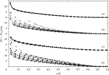
As with conventional inner scaling (using
 $u_{\unicode[STIX]{x1D70F}}$
and
 $\unicode[STIX]{x1D708}_{w}/u_{\unicode[STIX]{x1D70F}}$
), the mean velocity profiles do not scale using conventional outer variables (using
 $u_{\unicode[STIX]{x1D70F}}$
and
 $\unicode[STIX]{x1D6FF}$
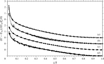
), as shown in figure 12, and the deviations increase with increasing stratification. Such trends are expected and follow those seen by Arya (Reference Arya1975). However, dividing the velocity deficit by
 $U_{\infty }\unicode[STIX]{x1D6FF}_{k}^{\ast }/\unicode[STIX]{x1D6FF}$
instead of
 $u_{\unicode[STIX]{x1D70F}}$
, as first suggested by Zagarola & Smits (Reference Zagarola and Smits1998a
) and Zagarola & Smits (Reference Zagarola and Smits1998b
), scales the data very well (see figure 13). Here
 $\unicode[STIX]{x1D6FF}_{k}^{\ast }$
is the kinematic displacement thickness, that is, calculated by ignoring changes in fluid density (3.2). Castillo & George (Reference Castillo and George2001) showed that this scaling also worked well for boundary layers with strong pressure gradients.
Stable boundary layer mean velocity profiles in conventional outer scaling. (a) Smooth-wall neutral; (b) smooth-wall stably stratified; (c) rough-wall neutral; (d) rough-wall stably stratified cases. Symbols for neutrally stratified cases as in table 1. Symbols for stably stratified cases as in table 2. Grey profiles signify greater uncertainty in
 $u_{\unicode[STIX]{x1D70F}}$
. Every fourth data-point shown for clarity.

Stable boundary layer mean velocity profiles in outer layer scaling of Zagarola & Smits (Reference Zagarola and Smits1998b
), using the kinematic form of the displacement thickness,
 $\unicode[STIX]{x1D6FF}_{k}^{\ast }$
. (a) Smooth-wall neutral; (b) smooth-wall stably stratified; (c) rough-wall neutral; (d) rough-wall stably stratified cases. Symbols for neutrally stratified cases as in table 1. Symbols for stably stratified cases as in table 2.

5.5 Turbulence profiles
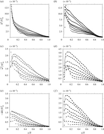
Turbulent stresses scaled by free stream velocity for (a,c,e) smooth and (b,d,f) rough walls. Near-wall data below
 $z_{10\,\%}$
shown with dotted lines. Conditions and symbols as in table 2.

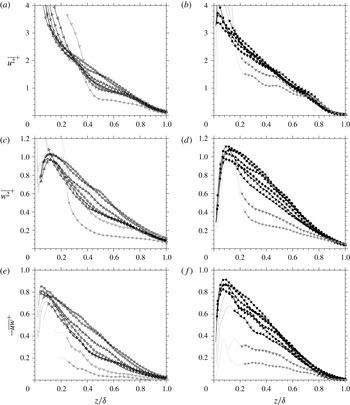
Previous experimental investigations of stably stratified boundary layers have always scaled the velocity variances using the free stream velocity, and for comparison purposes we begin in the same manner (see figure 14). As seen in the earlier studies, the turbulence intensities and shear stresses are progressively damped by increasing stability in an orderly way. The turbulent shear stress profiles retain much of their neutral shape, but the peak moves away from the wall slightly with increasing stratification, which is consistent with a thickening of the near-wall buffer region as found for the mean velocity profiles shown in figure 10. The near-wall results should be treated with some caution since the near-wall seeding level deteriorated at the higher levels of stratification. Nevertheless, the peak in the turbulent shear stress has been captured for all but the two strongest stratification cases, for both smooth and rough walls.
The increasing damping of turbulence by stability observed here follows the trends seen by Arya (Reference Arya1975) and Ogawa et al. (Reference Ogawa, Diosey, Uehara and Ueda1982), and the weaker stability cases of Ohya et al. (Reference Ohya, Neff and Meroney1997) and Ohya (Reference Ohya2001). At larger levels of stratification, however, Ohya et al. (Reference Ohya, Neff and Meroney1997) and Ohya (Reference Ohya2001) observed a preferential collapse of near-wall turbulence at a critical Richardson number, which they interpreted as signalling the start of a strongly stable regime, with this near-wall collapse as its defining characteristic. No preferential collapse of near-wall turbulence is observed in the current experiments. Rather, we see an orderly decrease in the turbulence across the boundary layer in this scaling, with a greater degree of damping in the outer layer than in the near-wall region.
Turbulent stresses in outer layer scaling for (a,c,e) smooth and (b,d,f) rough walls. Near-wall data below
 $z_{10\,\%}$
shown with dotted lines. Cases where
 $z_{10\,\%}$
lies significantly farther from the wall than the peak stress are shown in grey. Conditions and symbols as in table 2.

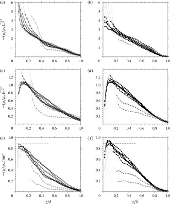
In an effort to discriminate between the (coupled) effects of Reynolds and Richardson number, we now present the turbulence profiles in conventional outer layer scaling (see figure 15), with the expectation that this will account for Reynolds number effects. As for the mean velocity profiles, the friction velocity was determined for all stratified cases using the near-wall maximum of the total shear stress (4.1) as the Clauser chart method could not be used for these cases. If we disregard the two cases with the highest wall temperatures for now, the turbulence profiles show improved agreement in this scaling compared to that using the free stream velocity (figure 14). We see that for both smooth and rough walls the peaks in the turbulent shear stress and the wall-normal turbulence decrease slowly with increasing stratification. The thickening of the viscous sublayer, seen in the mean velocity profiles, is also apparent in the profiles of streamwise variance for the smooth wall (figure 15
a), where the peak in near-wall turbulence moves away from the wall. For the rough-wall cases (figure 15
b), the growth in the peak in
 $\overline{u^{2}}$
is clear in this scaling, suggesting that the buffer layer is no longer completely subsumed by the roughness sublayer for the cases with the strongest stratification. It may be that under these conditions the flow can no longer be considered fully rough (Ligrani & Moffat Reference Ligrani and Moffat1986).
Only small changes in profile shape are noted for those cases where the peak shear stress scales with the wall stress. A slight kink is observed at
 $z/\unicode[STIX]{x1D6FF}=0.45$
for the strongest stratifications in the smooth-wall data that is not present in the rough-wall data. This kink is visible in the streamwise and wall-normal variances as well as in the turbulent shear stress. In contrast, the rough-wall profiles show no such localized change in slope. The location of the kink in the smooth-wall data suggests a connection with the mean velocity profile, which was primarily affected by stratification below
 $z/\unicode[STIX]{x1D6FF}=0.45$
for the smooth wall, whereas the effect of stratification was noticeable across the entire rough-wall boundary layer. Similarly, the local gradient Richardson number profiles show a slight increase at
 $z/\unicode[STIX]{x1D6FF}=0.45$
for the smooth-wall data, whereas the rough wall profiles increase more evenly. It appears that the local stratification profile has a small but marked effect on the shape of the turbulence profiles.
To explore the effects of fluid property variations, we can use a density-weighted scaling as is employed for compressible flows, Morkovin (Reference Morkovin and Favre1961) hypothesized that ‘the essential dynamics of compressible shear flows follow the incompressible pattern’ and is therefore expected to scale with variations in the local fluid density, provided the dynamic effects of density fluctuations can be neglected. Under these conditions, the turbulent stresses (
 $\unicode[STIX]{x1D70C}\overline{u^{2}}$
,
 $\unicode[STIX]{x1D70C}\overline{w^{2}}$
,
 $-\unicode[STIX]{x1D70C}\overline{uw}$
, etc.) should scale with the wall shear stress,
 $\unicode[STIX]{x1D70F}_{w}$
. In effect, this modifies the local friction velocity scale to become,
 $u_{\ast }=\sqrt{\unicode[STIX]{x1D70F}_{w}/\unicode[STIX]{x1D70C}}=\sqrt{\unicode[STIX]{x1D70C}_{w}/\unicode[STIX]{x1D70C}}\;u_{\unicode[STIX]{x1D70F}}$
. Figure 16 demonstrates that this Morkovin scaling improves the agreement of the profiles, especially near the wall. The scaling of the smooth-wall streamwise stresses in the middle of the layer is also seen to be improved.
Turbulent stresses in density-weighted (Morkovin) outer layer scaling for (a,c,e) smooth and (b,d,f) rough walls. Near-wall data below
 $z_{10\,\%}$
shown with dotted lines. Cases where
 $z_{10\,\%}$
lies significantly farther from the wall than the peak stress are shown in grey. Conditions and symbols as in table 2. Horizontal dashed line indicates the magnitude of the near-wall shear stress peak for the neutrally stratified case as predicted by Panton (Reference Panton1990).

The success of the Morkovin scaling for cases with weaker stratification suggests that similar conclusions can be drawn about the structure of weak to moderately stable boundary layers as are regularly drawn for compressible boundary layers since turbulence intensity is seen to reduce proportionally to the change in the wall shear stress and the effects of stratification are seen to be confined to small changes in the profile shape that appear correlated with the changes in mean stratification. The implications are twofold: dilatation effects do not appear to be important in the current experiments, despite large changes in density, and the turbulent structure of the boundary layer remains unchanged up until some critical stratification at which point the turbulence collapses and no longer scales with the wall shear.
Note that
 $u_{\ast }$
is defined in the same way as the velocity scale used in the ‘local scaling’ of Nieuwstadt (Reference Nieuwstadt1984; Reference Nieuwstadt and Hunt1985) since
 $u_{\ast }^{2}=(\unicode[STIX]{x1D70C}_{w}/\unicode[STIX]{x1D70C})u_{\unicode[STIX]{x1D70F}}^{2}=\unicode[STIX]{x1D70F}_{w}/\unicode[STIX]{x1D70C}=-\overline{uw}$
. The underlying arguments, however, are different because Morkovin scaling does not incorporate gravity or the turbulent heat flux, both a part of Nieuwstadt’s formulation. Instead, Morkovin scaling can be thought of as the appropriate scaling to account for variations in Reynolds number in a fluid of variable density where buoyancy has a negligible effect on turbulent structure.
5.6 Anisotropy
The ratio of root-mean-square velocity fluctuations in the streamwise and wall-normal directions, that is the anisotropy ratio
 $\unicode[STIX]{x1D70E}_{w}/\unicode[STIX]{x1D70E}_{u}$
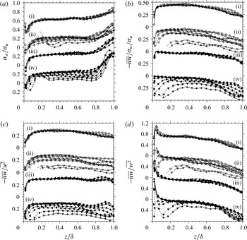
, is shown in figure 17. The results support the suggestion that the structure of turbulence is relatively insensitive to stratification for all but the two cases with the highest wall temperatures. The anisotropy ratio is insensitive to Reynolds number for both smooth- and rough-wall cases, with an almost constant value of approximately 0.6 over much of the layer, increasing toward the isotropic value of unity near the edge of the boundary layer, in line with the observations of Aubertine & Eaton (Reference Aubertine and Eaton2005). The anisotropy ratio only reduces significantly as the turbulence begins to collapse and no longer scales with wall shear, a behaviour that is consistent with the flattening of turbulent structures and dampening of the wall-normal momentum transport. These results agree with the atmospheric measurements by Kaimal et al. (Reference Kaimal, Wyngaard, Izumi and Coté1972), who observed changes in the ratio of the wall-normal to streamwise velocity spectra for
 $z/L\rightarrow 1$
, which in our case would occur in the outer layer and for the cases with the strongest stratification, where we also see changes in anisotropy.
The relative insensitivity of the anisotropy parameter to weak stability was also noted and discussed by Arya (Reference Arya1975). Stable stratification extracts energy directly from the
 $\overline{w^{2}}$
and
 $-\overline{uw}$
stresses but
 $\overline{u^{2}}$
is also reduced by the interaction of
 $-\overline{uw}$
and the mean velocity gradient. Previous direct numerical simulation studies have suggested that the reduction in the shear production of
 $\overline{u^{2}}$
is more important than the buoyant damping of
 $\overline{w^{2}}$
(Shah & Bou-Zeid Reference Shah and Bou-Zeid2014). Through the action of the pressure fluctuations, the energy is redistributed among all three components, explaining the relative insensitivity of this parameter to stratification. Similar conclusions can be drawn from the ratios of the streamwise and wall-normal stresses with the turbulent shear stress, also shown in figure 17. These results underline the marked decrease in turbulent transport efficiency as stability increases to levels that result in departures from wall shear stress scaling.
Evolution of the ratios of the turbulent stresses with thermal stratification. (i) Smooth-wall neutrally stratified, (ii) smooth-wall stably stratified, (iii) rough-wall neutrally stratified, (iv) rough-wall stably stratified cases. Symbols for neutrally stratified cases as in table 1. Symbols for stably stratified cases as in table 2.

5.7 Collapse
When we now consider the two strongest stratification cases, we see these cases exhibit a sudden and drastic reduction in turbulence levels in either conventional outer scaling or in Morkovin scaling. The shape of the profiles also depart significantly, indicating that this collapse is not simply due to increased uncertainty in the friction velocity. The absence of preferential damping of near-wall turbulence for the highest stability cases is again noted. This departure is seen to occur for bulk Richardson numbers exceeding 0.1 for the smooth wall, and about 0.15 for the rough wall. These values do not change significantly with free stream velocity, although the range of Reynolds numbers is small, and a weak Reynolds number dependence is not precluded. Ogawa et al. (Reference Ogawa, Diosey, Uehara and Ueda1985) observed the collapse of turbulence intensities for a smooth wall at similar bulk Richardson and Reynolds numbers as in the current study. Once the turbulence collapses, the remaining fluctuations are weak, patchy and not continuous. Nevertheless, the instantaneous PIV velocity fields (not shown here) indicate that weak individual hairpin structures persist even at the highest levels of stratification.
5.8 Quadrant analysis
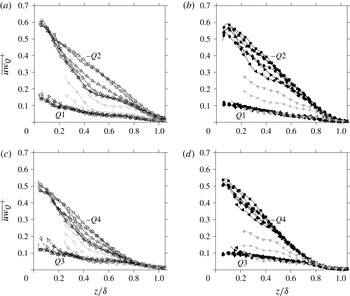
We have found that increasing stratification is associated with strong reductions in turbulent shear stress, leading to the collapse of turbulent production by mean shear. To explore this process more closely, we examine the quadrant contributions to the turbulent shear stress in the
 $u$
–
 $w$
plane, as formalized by Lu & Willmarth (Reference Lu and Willmarth1973). The results are presented in figure 18 in outer scaling. The motions that contribute to negative shear stress and positive turbulence production by mean shear, commonly termed ejections (
 $Q_{2}$
) and sweeps (
 $Q_{4}$
), are seen to be most affected by stratification, whereas the contributions to positive shear stress and negative production (
 $Q_{1}$
and
 $Q_{3}$
) are unaffected (relative to the local wall shear stress). At the same time, the effect on positive production motions is asymmetric, with ejections damped to a greater extent than sweeps. This is demonstrated more conclusively by examining the ratio of their contributions, as in figure 19, where we see that the greatest changes in their relative magnitude occurs in the outer layer. This ratio was found to be insensitive to changes in Reynolds number, at least for the neutral boundary layer (not shown here).
Quadrant contributions to the turbulent shear stress for (a,c) smooth- and (b,d) rough-wall cases. Conditions and symbols as in table 2. Grey profiles indicate those cases for which there is significantly greater uncertainty in the estimate of
 $u_{\unicode[STIX]{x1D70F}}$
.

Ratio of
 $Q2$
and
 $Q4$
contributions to the turbulent shear stress for (a) smooth and (b) rough surfaces. Conditions and symbols as in table 2.

The quadrant analysis thus suggests a weakening of turbulent motions that contribute to the production of turbulence, such as hairpin vortices. These vortices are inclined in the downstream direction, inducing ejections between the legs of the vortex and sweeps outside the legs. As hairpin vortices convect with a velocity close the local mean value (Adrian et al. Reference Adrian, Meinhart and Tomkins2000), quadrant analysis can be interpreted as revealing motions induced by a mean hairpin vortex at a given wall normal location. As ejections originate closer to the wall than a given hairpin head they must overcome a stronger temperature gradient than sweeps which originate further from the wall, potentially explaining our observed bias toward the damping of ejections.
5.9 Richardson number scaling and comparisons with the atmospheric surface layer
We now compare our results to those in the stable atmospheric surface layer, especially with respect to possible Reynolds number discrepancies. A number of different scaling systems have been proposed. The most renowned is MOST, which employs the fluxes of heat and momentum and the buoyancy parameter
 $\unicode[STIX]{x1D6FD}$
(
 $=g/T_{0}$
) as the primary governing variables (Monin & Obukhov Reference Monin and Obukhov1954). More recently, combinations of wall-normal velocity variance, temperature variance, wall-normal position (Sorbjan Reference Sorbjan2010) or the dissipation of TKE (Grachev et al.
Reference Grachev, Andreas, Fairall, Guest and Persson2015) have been combined with the Brunt–Väisälä frequency and
 $\unicode[STIX]{x1D6FD}$
to create new scaling systems. Of these, we choose to compare our results with those from the stable atmosphere in the gradient scaling of Sorbjan (Reference Sorbjan2010), where the velocity, temperature and length scales are defined in terms of the local temperature gradient, the buoyancy parameter, and the wall-normal distance. Newer formulations may be more advantageously constructed (see, for example, the discussion by Grachev et al. (Reference Grachev, Andreas, Fairall, Guest and Persson2015)), but the gradient-based formulation allows for a comparison with atmospheric results using variables that were measured in the current experiments (we do not have access to, for instance, accurate estimates for the dissipation rate or the turbulent heat flux).
In Sorbjan’s scaling the dependent variables, such as the turbulent shear stress and wall-normal variance, become functions of the gradient Richardson number. That is,
 $$\begin{eqnarray}\frac{-\overline{uw}}{U_{s}^{2}}=G_{t}(Ri),\quad \frac{\overline{w^{2}}}{U_{s}^{2}}=G_{w}(Ri),\end{eqnarray}$$
where the relevant velocity scale is
 $U_{s}=l_{0}N$
and
 $l_{0}$
is the mixing length. Sorbjan’s formulation employed two velocity components to account for rotation of the mean velocity direction due to Coriolis forces, but is similar to that shown here in any horizontal plane. Sorbjan’s scaling is consistent with MOST as the Richardson number is a function of
 $z/L$
in this theory. Sorbjan originally proposed that the mixing length increases linearly with wall-normal distance, that is,
 $l_{0}=\unicode[STIX]{x1D705}z$
. This scaling will fail further from the surface where the mixing length grows more slowly. Hence, Sorbjan (Reference Sorbjan2012) suggested employing the mixing length model of Blackadar (Reference Blackadar1962) such that
 $l_{0}=\unicode[STIX]{x1D705}z/(1+\unicode[STIX]{x1D705}z/\unicode[STIX]{x1D706})$
where
 $\unicode[STIX]{x1D706}$
is an external parameter usually modelled in terms of the Coriolis parameter and Rossby number.
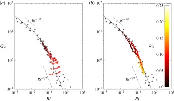
Root-mean-square of wall-normal velocity in the gradient-based scaling of Sorbjan (Reference Sorbjan2010). (a) Smooth- and (b) rough-wall symbols and conditions as in table 2. Data shown between
 $z^{+}>40$
and
 $z/\unicode[STIX]{x1D6FF}<0.7$
and
 $z>z_{10\,\%}$
. All data from the present wind tunnel measurements are coloured by bulk Richardson number
 $Ri_{\unicode[STIX]{x1D6FF}}$
. The solid line corresponds to the empirical correlation of atmospheric data (
 $+$
) presented by Sorbjan (Reference Sorbjan2010).

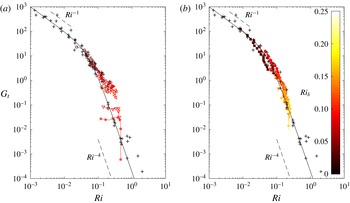
Examination of turbulent shear stress,
 $\overline{uw}$
, in the gradient based scaling of Sorbjan (Reference Sorbjan2010). (a) Smooth- and (b) rough-wall symbols and conditions as in table 2. Data shown between
 $z^{+}>40$
and
 $z/\unicode[STIX]{x1D6FF}<0.7$
and
 $z>z_{10\,\%}$
. All data from the present wind tunnel measurements are coloured by bulk Richardson number
 $Ri_{\unicode[STIX]{x1D6FF}}$
. The solid line corresponds to the empirical correlation of atmospheric data (
 $+$
) presented by Sorbjan (Reference Sorbjan2010).

Sorbjan (Reference Sorbjan2010) verified this gradient-based scaling using data from the Surface Heat Budget of the Arctic Ocean (SHEBA) experiment (Grachev et al.
Reference Grachev, Andrea, Fairall, Guest and Persson2008). The gradient Richardson number was chosen so that
 $0.5Ri_{e}<Ri<2Ri_{e}$
, where
 $Ri_{e}$
is the value of the gradient Richardson number predicted from the MOST similarity functions established by Grachev et al. (Reference Grachev, Andreas, Fairall, Guest and Persson2007, Reference Grachev, Andrea, Fairall, Guest and Persson2008), thus ensuring that the gradient-based results correspond closely to MOST. The wall-normal and shear stress data of Sorbjan (Reference Sorbjan2010) are shown in figures 20 and 21. Solid black lines indicate best-fit functions to the atmospheric data as given by Sorbjan (Reference Sorbjan2010). While the original study of Sorbjan (Reference Sorbjan2010) did not account for the wall-normal dependence of the mixing length, the data points represent the mean value for a small Richardson number bin, effectively averaging out any wall-normal dependence (within measurement error). The data of Sorbjan (Reference Sorbjan2010) were therefore found to provide the same empirical trends as the more complete scaling proposed by Sorbjan (Reference Sorbjan2012), which accounted for the wall-normal dependency directly. The comparison between atmospheric and experimental results using the data of Sorbjan (Reference Sorbjan2010) thus remains valid. The power laws observed at low
 $Ri$
are consistent with classical eddy viscosity/diffusivity models (sometimes known as
 $K$
-theory). The high
 $Ri$
power laws are empirical. As Sorbjan (Reference Sorbjan2010) pointed out, the error associated with these atmospheric data increase with
 $Ri$
.
The results for the stably stratified cases listed in table 2 are shown for the interval
 $z^{+}>40$
and
 $z/\unicode[STIX]{x1D6FF}<0.7$
(subject to
 $z>z_{10\,\%}$
), chosen to avoid regions with significant viscous effects and where small gradients cause large uncertainties in the gradient Richardson number. The mixing length model of Blackadar (Reference Blackadar1962) was used, as suggested by Sorbjan (Reference Sorbjan2012). The external parameter,
 $\unicode[STIX]{x1D706}$
, is conventionally modelled for the atmosphere in terms of the Coriolis parameter and Rossby number; an approach which is not valid for the current experiments. In the absence of better information, we choose
 $\unicode[STIX]{x1D706}$
to be the integral length scale of the streamwise velocity fluctuations,
 $L_{uu}$
for the data shown in figures 20 and 21 (see table 2). Despite the large field of view of the current experiments, it was necessary to fit exponential tails to the autocorrelation of velocity for large separations in order to obtain a more accurate estimate of the integral length. Williams (Reference Williams2014) gives further details.
We see that within the experimental uncertainty our results agree well with the atmospheric data prior to collapse (small to moderate Richardson numbers). This is especially true for the rough wall. The smooth-wall data diverge significantly only when the collapse of turbulent production is imminent, however the post-collapse rough-wall data continue to correspond closely to the trends of Sorbjan. The smooth-wall collapsed cases show a drop in scaled shear stress within the outer layer at high Richardson number but this is within the uncertainty of Sorbjan’s original study. This region is also the most sensitive to choice of mixing length model although using a linear model instead of that of Blackadar only caused deviations that are once again within the uncertainty of the atmospheric data. Other choices for
 $\unicode[STIX]{x1D706}$
were also investigated, such as the streamwise integral length scale of the wall-normal velocity fluctuations
 $L_{vv}$
, but they did not provide any particular improvement. Scatter of the higher stability smooth-wall data around the atmospheric correlation for the strongest stabilities may be the result of a small remaining dependence on wall-normal position not captured by Blackadar’s mixing length model.
The wide range of wall-normal positions over which agreement is observed suggests the broad validity of gradient-based and semi-local MOST scalings outside any region affected by viscosity. This promising correspondence also supports the proposal that wind-tunnel studies of stable boundary layers at low Reynolds number can yield results that can be directly applied to the understanding of the atmospheric surface layer.
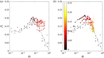
Estimate of the wall-normal proportion of the turbulent kinetic energy,
 $A_{w}^{\ast }=\unicode[STIX]{x1D70E}_{w}^{2}/(\unicode[STIX]{x1D70E}_{u}^{2}+\unicode[STIX]{x1D70E}_{v}^{2}+\unicode[STIX]{x1D70E}_{w}^{2})$
. (a) Smooth- and (b) rough-wall symbols and conditions as in table 2. Spanwise variance was estimated from
 $A_{v}$
correlation of atmospheric data by Sorbjan (Reference Sorbjan2010). Data shown between
 $z^{+}>40$
and
 $z/\unicode[STIX]{x1D6FF}<0.7$
and
 $z>z_{10\,\%}$
. All data from the present wind tunnel measurements are coloured by bulk Richardson number
 $Ri_{\unicode[STIX]{x1D6FF}}$
. The dashed line corresponds to the empirical correlation of atmospheric data
 $(+)$
presented by Sorbjan (Reference Sorbjan2010).

To this end, we examine the wall-normal fraction of TKE,
 $A_{w}=\unicode[STIX]{x1D70E}_{w}^{2}/(\unicode[STIX]{x1D70E}_{u}^{2}+\unicode[STIX]{x1D70E}_{v}^{2}+\unicode[STIX]{x1D70E}_{w}^{2})$
, which is often modelled as a function of stability parameters
 $z/L$
or
 $Ri$
(Schumann & Gerz Reference Schumann and Gerz1995; Zilitinkevich et al.
Reference Zilitinkevich, Elperin, Kleeorin, Rogachevskii and Esau2013). We have no measurements of the spanwise component of turbulence, but we can make an estimate from a fit to the spanwise proportion of the turbulent kinetic energy
 $A_{v}$
given by Sorbjan (Reference Sorbjan2010), resulting in an estimate, of the wall-normal fraction of TKE, which we denote as
 $A_{w}^{\ast }$
. The results are shown in figure 22, along with the atmospheric data of Sorbjan (Reference Sorbjan2010) (
 $A_{w}$
does not involve the mixing length and so a correction for wall-normal distance is not required). Our data correspond approximately with those of Sorbjan (Reference Sorbjan2010), who found a slight increase in
 $A_{w}$
above the neutral value for small to moderate Richardson numbers, before decreasing rapidly as wall-normal turbulence is suppressed at higher stability levels. The sharp increase in
 $A_{w}^{\ast }$
seen at the highest
 $Ri$
of each set is likely due to the increasing influence of measurement noise toward the edge of boundary layer as the stresses become small. The current experiments suggest a dependence on wall-normal distance, in addition to a dependence on Richardson number.
6 Critical stratification
It was noted in § 5.5 that for weak to moderate stability, turbulence intensities scale with the local shear stress and that the turbulent structure was insensitive to stability. For the cases with the strongest stratification, however, turbulent production was not sustained, as indicated by large changes in profile shape and departures from Morkovin scaling. These observations indicate the onset of a stability regimes where the local turbulence is no longer able adjust to changes in the local wall shear stress. We have used the term ‘collapsed’ to denote this regime to avoid confusion with previous definitions of a ‘strongly stable’ regime.
A number of measures have been proposed in the literature to delineate the collapse of turbulence and stability regimes. The most common measure (experimentally) is the critical bulk Richardson number, determined in this study to be approximately 0.1 and 0.15 for smooth and rough surfaces, respectively. No dependence on free stream velocity was seen in the current dataset, although the limited Reynolds number range does not preclude this possibility. The observed sensitivity to surface roughness (and possibly Reynolds number) means that the bulk Richardson number is not a suitable parameter for consistent delineation of these two regimes.
In this respect, Flores & Riley (Reference Flores and Riley2011) have suggested that Reynolds number based on the Monin–Obukhov length and the friction velocity provides a better measure of the collapse of turbulence. They observed collapse for
 $Re_{L}=Lu_{\unicode[STIX]{x1D70F}}/\unicode[STIX]{x1D708}_{w}\lesssim 100$
in simulations of turbulent open channel flow, suggesting that collapse occurs when the dynamic sublayer is not large enough to sustain a buffer region. Collapse was observed in the current experiments for
 $Re_{L}\lesssim 130\pm 60$
, based on estimates of the Monin–Obukhov length using the method described earlier. The Reynolds numbers based on wall temperatures on either side of collapse were averaged to obtain this estimate, and the error bound takes account of this averaging and variations between cases at different velocities. Given that Reynolds number drops precipitously prior to collapse and then decreases more slowly, this estimate may be biased to larger values. We conclude, therefore, that the current experiments are consistent with the bound in critical Monin–Obukhov Reynolds number suggested by Flores & Riley (Reference Flores and Riley2011). We did not observe any influence of wall roughness on this bound. For the current dataset, the parameter
 $L^{\ast }/k$
varied between 3 and 11 immediately after collapse, and it increased with tunnel flow velocity.
6.1 Stability theory of Schlichting
The linear stability analysis by Schlichting (Reference Schlichting1935) identified the gradient Richardson number evaluated at the wall,
 $Ri_{w}$
, as the parameter that separates regimes where small disturbances would grow or decay. The critical value of
 $Ri_{w}$
depends primarily on Reynolds number
 $(Re_{\unicode[STIX]{x1D6FF}_{k}^{\ast }}=U_{\infty }\unicode[STIX]{x1D6FF}_{k}^{\ast }/\unicode[STIX]{x1D708}_{w})$
and weakly on Froude number
 $(Fr^{2}=U_{\infty }^{2}/(g\unicode[STIX]{x1D6FF}_{k}^{\ast }))$
. Schlichting’s analysis includes mean profile curvature, which is an essential feature for properly characterizing the critical layer (Schlichting Reference Schlichting1979). By way of contrast, the analyses by Taylor (Reference Taylor1931) and Miles & Howard (Reference Miles and Howard1964) neglected profile curvature, but nevertheless led to the widely quoted critical Richardson number estimate of 1/4. Although Schlichting validated his analysis using a rather limited dataset obtained in a heated channel facility at Göttingen, his work seems to have been largely ignored. We will now compare our data with his predictions.
In figure 23 we show stability curves, as calculated by Schlichting, for three Froude numbers. We see that for Reynolds numbers less than about 1000, the critical Richardson number increases very quickly for small changes in Reynolds number, but it never exceeds a value of 1/24, which is the high Reynolds number asymptote for
 $Fr^{2}=0$
. With increasing Froude number, this value decreases, but it is only about 30 % smaller for
 $Fr^{2}=14.65$
.
We see from figure 23 that our weakly stable cases are in accord with Schlichting’s theory in that they lie within the dynamically unstable region where disturbances grow (within experimental error). Also, the majority of collapsed cases fall close to the critical Richardson number curves. The collapsed cases that lie within the unstable region are also the cases with the highest wall temperatures and bulk Richardson numbers and therefore have the greatest uncertainty in wall-gradient Richardson number and friction velocity. Overall, the correspondence between Schlichting’s theory and our experimental observations is encouraging for both smooth- and rough-wall cases.
Examination of flow conditions for weakly stable and collapsed cases and a comparison with the linear stability theory of Schlichting (Reference Schlichting1935). All ○ smooth- and ▵ rough-wall data are included. Closed symbols represent weakly stable cases; open symbols represent collapsed cases. Lines indicate Schlichting’s calculations of critical
 $Ri_{w}$
(gradient Richardson number evaluated at the wall) as a function of
 $Re_{\unicode[STIX]{x1D6FF}_{k}^{\ast }}$
for ——
 $Fr^{2}=0$
, – – –
 $Fr^{2}=5.86$
and – - – - –
 $Fr^{2}=14.65$
.

7 Conclusions
The effects of stable thermal stratification on the behaviour of turbulent boundary layer statistics were studied in an effort to better understand the underlying mechanisms, as well as give insight in the behaviour of the atmospheric surface layer.
For weak to moderate stability levels, reductions in streamwise and wall-normal turbulence were found to be proportional to reductions in the wall shear stress as the mean velocity profile (which obeys Zagarola–Smits outer layer scaling) progresses toward a less-full shape and the viscous layer thickens. Scaling the turbulent stresses using the wall shear stress helps to differentiate between Reynolds and Richardson number effects, and this delineation can be further improved by the use of a density-weighted friction velocity to account for changes in fluid density in the same manner as in compressible flows. Anisotropy ratios also suggest that the characteristic angle of turbulent structures is not altered significantly for weak to moderate stability. The anisotropy ratio is not sensitive to Reynolds number and does not change significantly with increasing stratification until turbulent production by mean shear is about to collapse.
With surface roughness, the mean velocity and temperature distributions were influenced by stratification across the entire boundary layer. The small differences observed in scaled turbulence profiles between the smooth and rough-wall results are likely to be due to changes in local stratification (that is, gradient Richardson number). Overall, the rough-wall results were found to follow the smooth-wall trends with the additional benefit of covering a wider range of Reynolds numbers. This observation also implies that the smooth-wall data were not affected by transitional effects.
For weak to moderate stability levels, the turbulence structure appears little affected by stratification, even as the mean velocity and temperature profiles undergo significant changes in shape due to decreased mixing. Within this regime, all changes in turbulence intensity appear consistent with the reductions in Reynolds number imposed by stability.
For strong stability levels, there is a marked change in the flow response. Vertical transport is reduced to the point where the turbulent production by mean shear collapses, and the turbulent stresses no longer scale with the wall stress. The collapse occurs at a bulk Richardson number of
 $Ri_{\unicode[STIX]{x1D6FF}}=0.1$
and
 $Ri_{\unicode[STIX]{x1D6FF}}=0.15$
for the smooth and rough wall, respectively. The shape factor of the mean velocity profile in this regime is similar to that seen in a laminar Blasius boundary layer. This stronger stability or collapsed regime is characterized by weak turbulence that no longer scales with the mean wall shear stress and where the large scale motions have a more horizontal structure. Quadrant analysis indicates that only the motions that contribute to positive turbulent production were influenced by stratification. Of these, the ejections, which move away from the wall, were found to be damped to a greater degree than sweeps, which move toward the wall.
This delineation of weak and strongly stable regimes based on the scaling of the turbulent stresses is in contrast to that proposed by Ohya et al. (Reference Ohya, Neff and Meroney1997) and Ohya (Reference Ohya2001), who characterized a strongly stable regime by the preferential near-wall damping of turbulence that appeared for bulk Richardson numbers above 0.25. Our results indicate instead that turbulence is preferentially damped in the outer flow, and continues to display a peak in intensity near the wall, even for the strongest stability cases where
 $Ri_{\unicode[STIX]{x1D6FF}}$
approaches 0.25.
The sensitivity to surface roughness of critical bulk Richardson number separating these two regimes could have implications for stable atmospheric flows over ice or salt flats compared to more typical rough earth surfaces. In addition, it seems likely that the bulk Richardson number is too crude a measure to delineate regimes over a wide range of conditions. The current results are instead consistent (within experimental error) with collapse occurring at a critical Monin–Obukhov length-based Reynolds number of close to 100, as suggested by Flores & Riley (Reference Flores and Riley2011) and the linear stability theory of Schlichting (Reference Schlichting1935), where the critical wall-gradient Richardson number is a function of Reynolds and Froude numbers. Schlichting’s critical wall-gradient Richardson number has a maximum of 1/24 for
 $Fr=0$
and reduces with Reynolds number and increasing Froude number. Both of these measures are preferred to the bulk Richardson number for the delineation of stability regimes as they involve fluxes and gradients taken at the wall.
Finally, good correspondence was observed between the current experiments and atmospheric data in the gradient Richardson number scaling of Sorbjan (Reference Sorbjan2010), at least for locations outside the near-wall viscous region. This result suggests that the effects of Reynolds number on turbulent velocity statistics can be largely accounted for through known scaling techniques and that many aspects of the atmospheric surface layer can be investigated using results from relatively low Reynolds number stably stratified laboratory experiments. Reynolds number effects however may continue to influence the collapse of turbulence at the highest stabililities, as we show in § 6.1, and for other properties such as the heat transfer coefficients of rough walls (Li et al. Reference Li, Bou-Zeid, Anderson, Grimmond and Hultmark2016).
Acknowledgements
This work was supported in part by the Cooperative Institute for Climate Science (CICS) at Princeton University. E.B.-Z. was also supported by the National Science Foundation’s Division of Physical and Dynamic Meteorology under AGS-1026636. The authors would like to thank Dr C. Ansorge for providing us with his German-to-English translation of the 1935 paper of Schlichting.