Age at Arrival: Historical Setting and Related Literature

The Age of Mass Migration (1850–1913) is often split into two sub-eras based on the geographical shift of flows from Northern and Western Europe (“Old” sources) to Southern and Eastern Europe (“New” sources) in the late 1880s. At around the same time there was also a shift in family composition from intact households (including many children) to unattached males, lowering the fraction of child arrivals (Baines Reference Baines1995; Hatton and Williamson Reference Hatton and Williamson1998). Illustrating this shift in the late nineteenth century, Michael J. Greenwood (Reference Greenwood2007) reports that the percentage of those under 14 in the inflow from major European sources dropped from a high of 25 percent in 1884 to a low of 11 percent in 1895. This shift away from family and child migration is associated with younger males taking advantage of the decreasing costs of travel due to the diffusion of steam technology and migration networks (Cohn Reference Cohn2009; Gould Reference Gould1980).

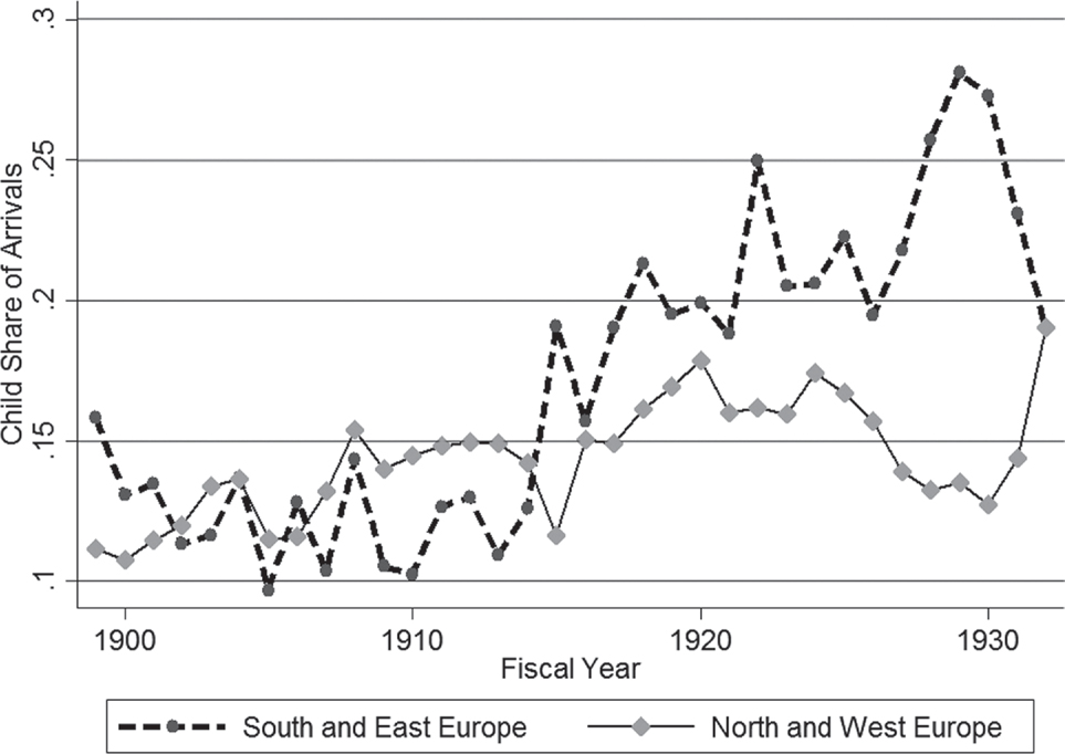
Our data cover migrants who entered through Ellis Island between 1892 and 1924, a period when child arrivals were slowly making up a larger share of arrivals (see Figure 1).Footnote ² Children were still a small, but increasingly important, part of the inflow: overall, the fraction of child arrivals increased from 10 to 14 percent before WWI to slightly above 15 percent in the following decade. Some of this increase is due to several shocks to the immigration system, such as the cut-off of flows during WWI, the Literacy Act of 1917, and the immigration quotas laws of 1921 and 1924. While U.S. policy significantly restricted the overall flow, child arrivals were favored under these policies since those under 16 were not subject to the literacy test, and children joining a naturalized family member were given preference under the quota system.Footnote ³ Consistent with policies favoring children more than single adults, the countries that were more restricted under the quotas and literacy test (in Southern and Eastern Europe) had a relative increase of children in their flow.

Figure 1

Child Share of Immigrant Inflows to the United States, 1899–1932

Notes: Fiscal years are between 1 July and 30 June. Child arrivals are those under the age of 14 between 1899 and 1916 and under the age of 16 between 1917 and 1932. See Footnote 2 for definition of arrival.Sources: Annual Reports of the Commissioner General of Immigration, 1899–1932.

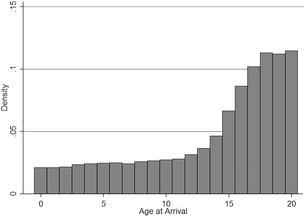
While child arrivals were less than 20 percent of arrivals in the early twentieth century, they were about 30 percent of the migrant stock, partially because they were more likely to remain rather than return home.Footnote ⁴ This can be directly seen in return flow records where children were underrepresented on out-going ships relative to the migrant stock; moreover, arrival records show that families with children were more likely to plan to stay in the United States permanently than single arrivals (Ward Reference Ward2017). Yet not all young migrants arrived with family members; this is indirectly seen in the distribution of age at arrival in the migrant stock in Figure 2.Footnote ⁵ While there were about the same proportion of arrivals at age one as for age 12, there were much more arrivals aged 13 and above, perhaps because teenagers were more likely to migrate by themselves. If older arrivals came individually while younger arrivals came as part of a family, then older teenagers could be selected from a different part of the source country human capital distribution; therefore, it will be important to estimate the effect of age at arrival with an empirical strategy that accounts for changing unobservables across the arrival age distribution.

Figure 2

Distribution of Immigrant Age at Arrival in the 1900–1930 U.S. Censuses

Notes: The sample is limited to those who arrived between 1899 and 1930 to match with Figure 1. The distribution is estimated after applying the person weight available from IPUMS.Sources: 1 percent samples of the 1900–1920 Censuses, 5 percent sample of the 1930 Census (Ruggles, Genadek, Goeken, et al. 2017).

Early twentieth century officials recognized the importance of age at arrival for successful assimilation; of special concern was whether older arrivals were falling behind in school. The 1910 Dillingham Commission Reports on The Children of Immigrants in Schools showed that 43 percent of children who arrived under age six were behind their grade level, compared with 92 percent of those who arrived at ten years or older. The authors argued that “the child who comes to this country before he reaches school age often has an opportunity to adjust himself to his new surroundings and in some cases learn the language through contact with other children before entering school” (Immigration Commission 1910, p. 51). In response to this trend of child arrivals being poorly educated, states passed compulsory schooling laws to educate immigrant children who arrived from countries without a compulsory educational system (Bandiera, Mohnen, Rasul, et al. Reference Bandiera, Mohnen and Rasul2016).

Despite early twentieth century officials’ interest in age at arrival, the Congressional Report is one of the only studies that separates historical migrant outcomes by arrival age.Footnote ⁶ Others that account for age at arrival often group all child arrivals into a single category. Both Chris Minns (Reference Minns2000) and Timothy Hatton (Reference Hatton1997) show that those who arrived under the age of 16 had higher income levels and better-paid occupations than adult arrivals, consistent with a negative effect of age at arrival and longer exposure to the European environment. On the other hand, Ran Abramitzky, Leah Boustan, and Katherine Eriksson (Reference Abramitzky, Boustan and Eriksson2014) show that assimilation rates were similar whether one keeps or drops those who arrived under the age of ten, but since they do not isolate the sample to only child arrivals, the difference in assimilation for child arrivals is unclear. We improve on this limited literature by estimating the effect of age at arrival across all ages, rather than grouping all child arrivals together. We also use an empirical strategy that controls for household-invariant unobservables that are correlated with age at arrival and with economic outcomes, which is important in today’s studies on age at arrival (Clarke Reference Clarke2016).

In contrast to the scarcity of historical studies, several modern-day studies estimate the effect of age at arrival on adult outcomes with high-quality data.Footnote ⁷ The most credible method to identify the age-at-arrival profile uses sibling fixed effects. This requires a large amount of data and therefore has been primarily studied using Swedish and Norwegian administrative records (Böhlmark Reference Böhlmark2008; van den Berg, Lundborg, Nystedt, et al. Reference Van den Berg, Lundborg and Nystedt2014). Outside of Northern Europe, there are few studies that identify the effect of age at arrival with siblings. Raj Chetty and Nathaniel Hendren (Reference Chetty and Hendren2017a, Reference Chetty and Hendren2017b) use U.S. tax records to show that variation in age at migration across counties has a large effect on adult outcomes, implying that childhood environment varies widely across counties in the United States. We follow this sibling fixed effects approach to estimate the importance of childhood environment for immigrants from the past.

Linking Ellis Island Records to the 1940 Census

The main dataset used for estimation comes from linking two large data sources: Ellis Island records from 1892 and 1924 and the preliminary full-count 1940 Census available at IPUMS (Ruggles, Genadek, Goeken, et al. Reference Ruggles, Genadek and Goeken2017). The Ellis Island records have been digitized and are searchable online; note that this source is the same one used by Oriana Bandiera, Imran Rasul, and Martina Viarengo (Reference Bandiera, Rasul and Viarengo2013) and Yannay Spitzer and Ariell Zimran (Reference Spitzer and Zimran2017).Footnote ⁸ While the clear advantage of the Ellis Island records is that they include millions of observations, there are a few disadvantages. One is that not every variable in the arrival records is digitized, such as occupation, relationship status, or height. Moreover, the Ellis Island records include both immigrants and non-immigrants; non-immigrants are other entrants such as business travelers, tourists, or those traveling through to another country. However, we are only interested in those who we can locate in the 1940 Census, and thus those who have stayed permanently (and survived) until 1940.

Our population of interest in the Ellis Island records is brothers who are single and arrived between the ages of zero and 20. For this population (who are primarily European), we collect first name, last name, age, date of arrival, place of last residence, and ethnicity. We identify brothers as immigrants who are listed next to each other with the same last name and are less than ten years apart in age, although we do not have their relationship listed in the data. The key variable of interest from these records is age, which we wish to attach to their adult observation in the 1940 Census. For a discussion of the assumptions we made in cleaning the data, please see Online Appendix B. After cleaning, we have 397,003 brothers who can be linked to the 1940 Census.

We link these brothers to the 1940 U.S. Census using a match on first name, last name, country of birth, and year of birth in a 3-year range.Footnote ⁹ We find potential matches based on having an exact NYSIIS match on first and last name; however, we choose the best match based on the smallest sum of the absolute difference in year of birth, Jaro–Winkler distance in first name and Jaro-Winkler distance in last name.Footnote ¹⁰ Catherine Massey (Reference Massey2017) shows that this method of ranking matches is reasonable for improved match rates and reduced false positives. For more detail on the linking process, see Online Appendix C.

It is possible that our linking methodology incorrectly links some people, which would induce measurement error and bias our sibling fixed effects estimates toward OLS estimates (Bailey, Cole, Henderson, et al. Reference Bailey, Cole and Henderson2017). However, as we will show in robustness checks, our results do not change when limiting our sample to higher-quality links in terms of closer matches in first and last name strings and year of birth. The results are also robust in an alternative sample where links are chosen based on a predicted match score calculated from a hand-linked sample of immigrants, a method that is related to the linking strategy described by James Feigenbaum (Reference Feigenbaum2016).Footnote ¹¹ Overall, we are confident that our results are not driven by link quality.

We take one extra step when linking the datasets because we start with arrival records unlike others who link from census to census. We are concerned that some immigrants may have changed their first name to be more “American” after arrival; for example, from Giuseppe to Joseph or Pietro to Peter. Costanza Biavaschi, Corrado Giulietti, and Zahra Siddique (Reference Biavaschi, Giulietti and Siddique2017) show that name changes occur for 32 percent of their sample of naturalization records in New York and that name changes were more common for Southern and Eastern Europeans. To account for this possibility, we Americanize the first names in our dataset of arrival records and the first names in the census records. This will allow us to match Giovanni at arrival to John in the census, but also to match Giovanni (Americanized to John) at arrival to Giovanni (Americanized to John) in the census in case Americanization did not occur. We do this with a list of more than 28,000 variants of first names based on information at behind thename.com.Footnote ¹² The Americanization process improves our linking rates by about 35 percent, but, as we will show in a later robustness check, our results do not substantially change if we do not Americanize first names.

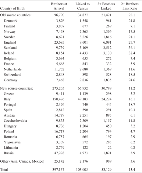
The starting sample of 397,137 brothers is successfully linked for 103,005 individuals in the 1940 Census using our main linking approach, or 25.9 percent of arrivals. Since the main empirical strategy exploits variation within brothers, we drop individuals where one brother was linked and another was not. This restriction gives us a final sample of 53,129, or 13.4 percent of our original set of brothers.

Table 1 shows the linking rates by country of birth and demonstrates a common pattern in the literature where we are less likely to link Southern and Eastern Europeans relative to Northern and Western Europeans (Abramitzky, Boustan, and Eriksson Reference Abramitzky, Boustan and Eriksson2014; Ward Reference Ward2018). Clearly, our linked sample is not a random sample of foreign-born brothers. We are not able to test for the representativeness of the sample on occupation or literacy compared to all Ellis Island arrivals since these variables are not digitized. Yet we would rather test for representativeness according to the 1940 Census since the Ellis Island records include many non-immigrants and thus any difference between our linked sample and those in the Ellis Island data would reflect both selection into permanent migration and selection into the linked sample. However, we also cannot test for representativeness according to the 1940 Census because it does not separate immigrants by cohort or age of arrival, once again making it unclear whether any differences are due to biases from the linking process or because the linked data has younger arrivals.Footnote ¹³

Table 1

Birthplace Composition in Ellis Island Data Linked to the 1940 Census

Notes: The empirical strategy uses sibling fixed effects, so we only keep sets of brothers where at least two are successfully linked (2+ Brother Linked column).

Sources: Linked sample of brothers from Ellis Island records to the 1940 Census.

Most linked samples that use a similar linking methodology are found to be slightly higher skilled than the underlying population and only show a strong bias in country of birth (Abramitzky, Boustan, and Eriksson Reference Abramitzky, Boustan and Eriksson2014). New source countries are less likely to be linked to the 1940 Census than Old sources because of common names, return migration, misspelled names, or names that are not captured in our list of Americanized names. To account for this bias, we reweight the sample to reflect the migrant stock by country of birth in 1940, although this reweighting does not drive our results.Footnote ¹⁴

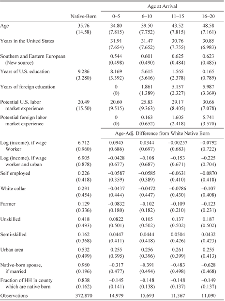
Table 2 shows the descriptive statistics of the linked sample of brothers and the 1 percent sample of white natives in the 1940 census, illustrating the gaps in economic and social outcomes between immigrants and natives. We compare our immigrants to white natives on several outcomes, including years of completed education, occupation, and wage income. Note that whenever we use wage income, in this table or in later regressions, we exclude self-employed workers since business and farm income are not included in the 1940 Census.

Table 2

Descriptive Statistics of Linked Sample of Brothers

Notes: Native born are white males restricted to the same birth cohorts are the immigrant sample. Total education and potential labor market experience is split under the assumption that individuals enter school at age six and continuously attend for their full years of schooling (see Footnote 26). The outcomes are age-adjusted residuals after predicting life-cycle variation with the native born (see equation (1) in text). There is missing information for some of these variables. Specifically, 17,152 do not have a positive log income, 1,538 have missing education, 5,226 have missing self-employment, and 3,225 have a blank occupation. HH stands for household heads.

Sources: Linked sample of brothers from Ellis Island records to the 1940 Census and 1 percent sample of 1940 Census.

The migrants in our sample have been in the United States for an average of about 31 years. Therefore, those who arrived between age zero and five are on average 34 years old in 1940, while those who arrived between ages 16 and 20 are on average 49 years old in 1940. Considering these differences in age, it will be important to adjust for age when examining differences between immigrants and natives, which we show in the bottom half of the table. After adjusting outcomes based on white natives’ life-cycle profile, Table 2 shows that there is a strong negative gradient to age at arrival for many variables.Footnote ¹⁵ For example, zero-year-old arrivals earned 9.5 percent more than natives, while 16–20 year old arrivals earned 7.9 percent less. Note that children arriving early enough have earnings that are higher than natives of the same age, perhaps implying that childhood environment may explain the entire native-immigrant wage gap for older arrivals. Yet part of the reason why younger arrivals earned more than white natives overall was because they located in urban areas. Table 2 shows that when limiting the sample to those only in urban areas, then zero-year-old arrivals earned 4.3 percent less than natives. Nevertheless, when limiting the sample to urban areas, the same pattern holds where older arrivals had a larger wage gap with natives compared with younger arrivals.

One explanation for the change in income gap across age at arrival is that older arrivals were exposed to source country conditions for a longer period. On the other hand, the change may be due to selection bias such that older arrivals had worse outcomes because they came from lower income or educated families. Instead of estimating the age-at-arrival profile using variation across families, we will estimate the profile using variation within family to control for unobserved family-invariant variables (such as parental education and income) as described in more detail in the next section.

Empirical Strategy and Identification

The first challenge when estimating the effect of age at arrival on immigrant outcomes is a standard one of collinearity: it is not possible to simultaneously estimate the effect of age at arrival, age, and years in the United States because they are linearly dependent.Footnote ¹⁶ We follow the standard practice of using natives to identify the life-cycle profile (or aging effect), and then estimate whether age at arrival influences deviations from this profile (Borjas Reference Borjas1985).Footnote ¹⁷ We take the two-step approach used by Joseph Schaasfma and Arthur Sweetman (Reference Schaafsma and Sweetman2001): first, we estimate an auxiliary regression to identify the age-earnings profile using only white native-born individuals (superscript nb) from the same birth cohorts as our immigrant sample:

(1) $\ln \left( {incom{e_i}} \right)\lambda _a^{nb} + {\varepsilon _i}.$

The income-age profile is modelled using a full-range of age fixed effects. We then estimate whether deviations from the native age-earnings profile are related to the immigrant’s age at arrival, while controlling for other factors such as years in the United States:

(2) $\ln \left( {incom{e_i}} \right) - \widehat \lambda _a^{nb} = g\left( {Age\,At\,Arriva{l_i}} \right) + h\left( {Years\,in\,U{S_i}} \right) + {\upsilon _i}.$

Therefore, this equation shows that the estimated effect of age at arrival on outcomes is the effect of age at arrival on the native-immigrant gap.Footnote ¹⁸ The method essentially estimates the effect of differences in age at arrival on the difference between natives’ and immigrants’ log income by age.

The second problem with estimating the effect of age at arrival is selection bias: immigrants who arrive at older ages may differ from those who arrive at younger ages in unobservable ways. For example, families with a strong preference for improving their child’s education may have immigrated to the United States with children at younger ages prior to school entry. In this case, an estimated age-at-arrival effect may capture family preferences for investment into children and lead to a negative age-at-arrival profile if families with younger children are positively selected relative to families with older children. Indeed, in present-day data, those immigrating with younger children also tend to have higher education levels than those migrating with older children (Clarke Reference Clarke2016).

To address issues of selection bias when comparing immigrants across families, we compare immigrants within the family (i.e., we compare brothers). The regression therefore changes to

(3) $\ln \left( {incom{e_{ih}}} \right) - \widehat \lambda _a^{nb} = g\left( {Age\,At\,Arriva{l_{ih}}} \right) + {\phi _h} + {\upsilon _{ih}},$

where the key addition is the sibling fixed effect φ_h. Therefore, we relate the variation of native-immigrant income gap within siblings to the variation in age at arrival within siblings. Including household fixed effects controls for many household-invariant factors such as parental preferences for education or childhood investment, parental wealth, father and mother’s education, culture, family structure, and country of origin. Note that this strategy compares individuals from the same arrival cohort with the same number of years in the United States, so these other variables of interest in the assimilation literature are dropped from the equation.

We use a non-parametric approach and code age at arrival into two-year bins (arrived between zero and one, between two and three, etc.) up until arrival at age 18.Footnote ¹⁹ This specification allows us to capture a variety of slopes in the profile such as the age-at-arrival profile being flat until ages eight to ten and decreasing afterwards, reflecting language acquisition or other effects of this critical period (Bleakley and Chin Reference Bleakley and Chin2004; van den Berg, Lundborg, Nystedt et al. Reference Van den Berg, Lundborg and Nystedt2014). Alternatively, the slope could be steepest for arrival ages under five, reflecting the importance of human capital development at very young ages (Almond, Currie, and Duque Reference Almond, Currie and Duque2017). Note that we do not control for any post-arrival outcome, such as geography or marital status, because location could be an outcome of age at arrival (Bleakley and Chin Reference Bleakley and Chin2010).

For the regression to estimate a causal relationship, the identifying assumption is that age at arrival is not correlated with unobservables that vary within the family and also affect income. Unfortunately, we are unable to include other control variables that may bias our estimates due to the limited information in arrival records. The primary concern is birth order: birth order may affect adult outcomes through general birth order effects, and birth order is also correlated with age at immigration. It is also possible that parents may time immigration to be optimal for the younger child (e.g., immigrate just prior to school entry) such that younger arrivals would have better outcomes due to unobservable parental investment into younger children. Unfortunately, we only observe birth order according to the arrival records, which ignores older siblings who may have stayed in the source country (Abramitzky, Boustan, and Eriksson Reference Abramitzky and Boustan2013). Since birth order is not exactly observed, we do not control for it in our main specification; nevertheless, we show in a robustness check that the results are robust to controlling for birth order.

There are a few threats to the external validity of our estimates, where they may not apply to all child immigrants during the Age of Mass Migration. First, we only identify the age-at-arrival profile with brothers rather than single arrivals; these estimates may differ if there is an extra disruptive effect for older brothers who have to take care of their younger brothers, though the sizes of our effects are likely too large for this to be driving our result. Another possible bias is that we mismeasure the effect of age at arrival for the entire population due to selective return migration (Abramitzky, Boustan, and Eriksson Reference Abramitzky, Boustan and Eriksson2014; Ward Reference Ward2017). Our sample only consists of brothers who remained in the United States; however, if one brother stayed and another returned home, then they would not be included in our sample. If older arrivals were more likely to return home and older arrivals also earned less income, then we would understate the negative effect of age at arrival. A similar story and bias would apply in the case of selective mortality. Finally, our estimates do not apply to all arrivals since we only link those who arrived through Ellis Island, which primarily misses entrants from Asia, Canada, or Mexico.Footnote ²⁰ Therefore, the reader should keep in mind that our results come from brothers who arrived at Ellis Island between 1892 and 1924 and survived until the 1940 Census.

The Effect of Age at Arrival on Economic Outcomes

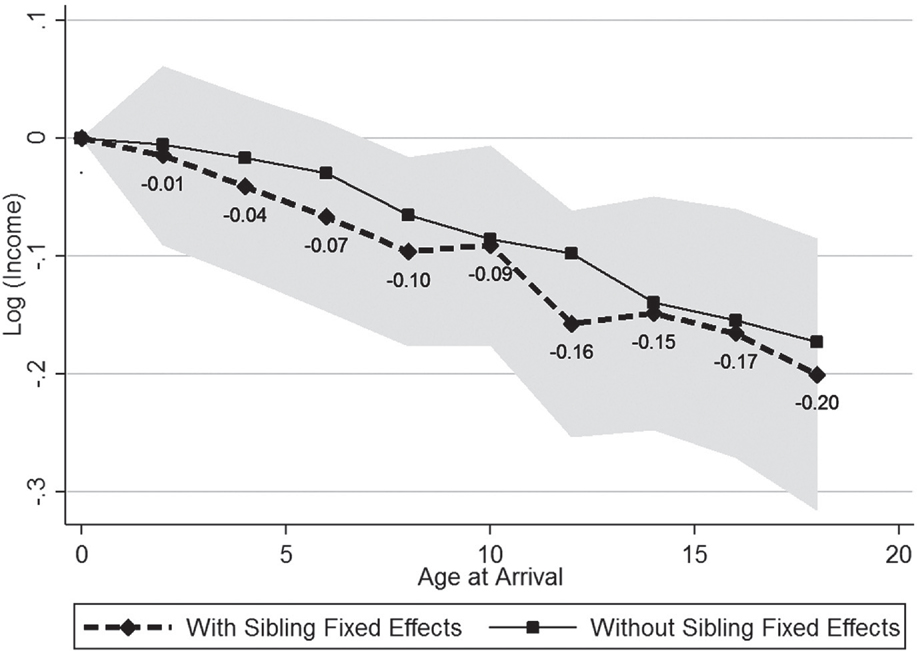
We estimate the effect of age at arrival with the brothers fixed effects specification and plot the coefficients in Figure 3. The plotted coefficients estimate the difference in native-immigrant wage gap relative to the native-immigrant wage gap for zero- to one-year-old arrivals. The results show a strong negative slope for age at arrival such that the native-immigrant wage gap was 17 log points (or 15.6 percent) more negative for a 16-year-old arrival compared with the wage gap for an infant arrival. If one assumes that the return to education was 6.5 to 7.9 percent in 1940 (Clay, Lingwall, and Stephens Reference Clay, Lingwall and Stephens2016), then having a full childhood in the United States was equivalent to receiving more than two additional years of schooling.

Figure 3

The Negative Effect of Age at Arrival on the Native-Immigrant Gap in Wage Income In 1940

Notes: The dependent variable is the age-adjusted gap in log wage income between immigrants and natives. Self-employed workers are dropped. The figure shows the estimated fixed effects for age at arrival with age at arrival of zero and one being the excluded group. The shaded area is the 95 percent confidence interval when using sibling fixed effects. Standard errors are clustered at the household level.Sources: Sample of brothers linked from Ellis Island records to the 1940 Census.

This result is consistent with the U.S. childhood environment yielding a higher return than the childhood environment in the source country. The pattern could be due to a higher-quality education or health environment in the United States; yet at the same time, the quality of the health environment may not have been higher in the United States. For example, Katherine Eriksson and Gregory Niemesh (Reference Eriksson and Niemesh2016) show that children of black migrants during the Great Migration had higher infant mortality rates relative to children of non-migrants due to poor health conditions in northern cities. However, for states for which we have data at the turn of the twentieth century, infant mortality rates for foreign-born mothers were less than those for African Americans and similar to the rates in many European sources (Preston and Haines Reference Preston and Haines1991, Tables 2.3 and 3.1). Ultimately, it is unclear whether migrating from Europe led to a lower quality health environment in the United States. Another possibility is that the U.S. environment was not better objectively, but rather that its education system trained individuals specifically for the U.S. labor market.

Despite the creation of the new linked sample of brothers, the age-at-arrival profile estimated without sibling fixed effects is within the standard errors of the profile estimated with sibling fixed effects.Footnote ²¹ This result suggests that family-invariant unobservables such as parental preferences and education do not strongly bias the age-at-arrival profile estimated with OLS. However, it is also possible that we do not detect a difference in profiles between the methodologies due to errors in the linking process, which would bias the sibling fixed effects result towards the OLS result. This is likely not the case since we find the same result when limiting the sample to higher-quality links. In Online Appendix Table A2, we keep the top 50 percent of links in terms of quality of match based on closeness of name and year of birth and show that even with higher quality links, the sibling fixed effects method estimates a profile that is within the 95 percent confidence interval of the profile estimated with our main sample. We also show that if one links immigrants in a method related to Feigenbaum (Reference Feigenbaum2016), then the estimated profile is also within the confidence interval of the profile estimated with our main sample (see Online Appendix E for more detail).

The negatively-sloped age-at-arrival profile appears to be linear; however, standard errors are wide so the profile may not truly be linear. Nevertheless, if one models the age-at-arrival effect to be constant across ages, then the effect of arriving one year later leads to a 1.1 percent more negative wage gap with white natives. A linear age-at-arrival profile would go against expectations in two ways: first, others have found a steepening of the profile around the ages of 8 to 11 due to critical periods of language acquisition or health development (Bleakley and Chin Reference Bleakley and Chin2004; van den Berg, Lundborg, Nystedt, et al. Reference Van den Berg, Lundborg and Nystedt2014). Our estimate does show a dip in income between age 8 and 14, consistent with a critical period effect, but we cannot statistically detect a break in the slope. We also do not detect a steeper slope for ages under five, which may be surprising given the large returns to improved childhood environment during very young ages (Almond, Currie, and Duque Reference Almond, Currie and Duque2017); yet this may reflect the countervailing effects of a lower quality health environment in the United States relative to Europe.

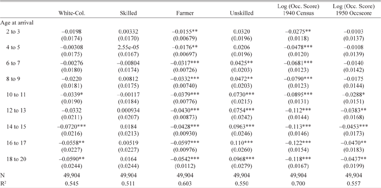
Not only did arriving at an older age cause the native-immigrant gap to be more negative, but it also caused immigrants to enter lower skilled occupations relative to natives.Footnote ²² Table 3 shows that arriving at an older age increased the likelihood of entering an unskilled job and lowered the likelihood of holding a white-collar job. To provide a summary measure of the effect of age at arrival on occupation, the last two columns estimate the effect on occupational score and show that the native-immigrant gap for 16-year-old arrivals was five to 12 log points more negative than for infant arrivals.Footnote ²³ Since the magnitude of the effect on occupation score is less than the magnitude of the effect on income (17 log points), this suggests that age at arrival affected both occupation and income within occupation. Given these effects of age at arrival on income and occupation, it may be that age at arrival also affected other dimensions such as labor supply, but as shown in the Online Appendix, we find no effect of age at arrival on labor force participation or weeks worked (Table A3).Footnote ²⁴

Table 3

Effect of Age at Arrival on Occupations

Notes:

^*** p<0.01

^** p<0.05

^* p<0.10

The occupational score in the second to last column is the logged occupation based on mean wages in the 1940 Census (see Online Appendix D). The last column is the log occupational score based on the variable occscore in IPUMS. The excluded group is arrivals aged zero and one. Brothers fixed effects are included in each column. Standard errors are clustered by household.

Sources: Linked sample of brothers from Ellis Island records to the 1940 Census.

We check the robustness of the age-at-arrival profile when controlling for observed birth order. Recall that observed birth order may not reflect the true birth order since we do not observe family members left behind in the source country. In each specification, the age-at-arrival profile is unchanged, and the birth order effects are statistically insignificant. Another concern is that including immigrants who arrived aged older than 16 may bias results since older arrivals may have decided on their own to immigrate while younger arrivals had less choice. To account for this, we re-estimate the age-at-arrival effect when dropping those who arrived older than age 15, and find no difference in the estimated income profile. Finally, we test for the robustness of our linking process to the Americanization process by relinking our data without Americanizing names. The estimated effects without the Americanization process have less precision (see Table A7) but reaffirm the negative effect of age at arrival on adult labor market outcomes. These robustness checks are shown in Online Appendix Tables A5–A7.

Potential Mechanisms for the Age-At-Arrival Effect

Arriving at an older age negatively affected labor market outcomes later in life, but through which channels? The potential mechanisms are numerous, but to name a few: the system of education changed across countries; parental resources may have improved after the move and thus investment into the child also improved; and younger arrivals may have socially adapted at a quicker rate. In this section, we estimate how age at arrival was related to these potential mechanisms.

Total Years of Education

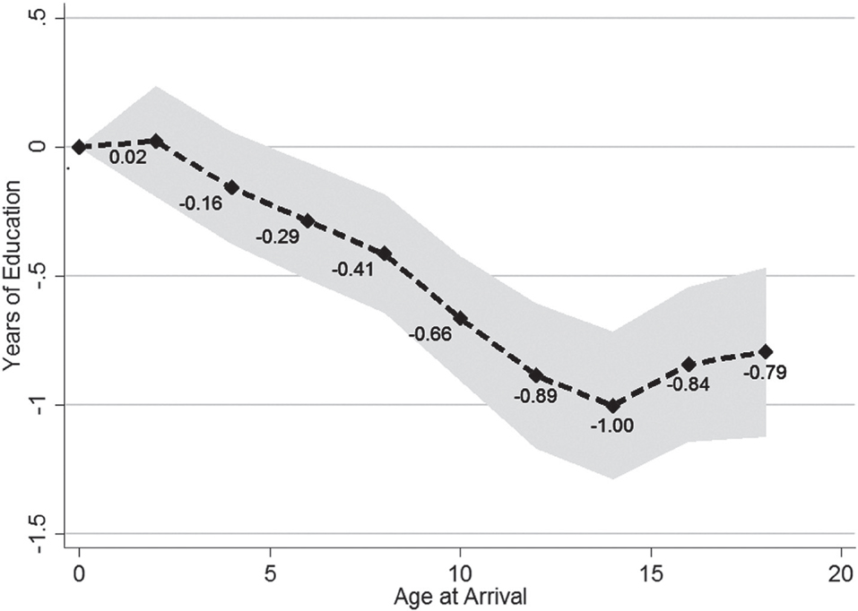
First, we test whether age at arrival affected the total years of educational attainment. When we run the same age-at-arrival regression with native-immigrant gap in education as the dependent variable, we find that the gap for older arrivals was larger than the gap for younger arrivals by one year (see Figure 4). The education profile looks similar to the income profile in that they are both negatively sloped, suggesting that education could be a primary channel for the age-at-arrival effect on income. However, in contrast with the income profile, the education profile becomes flat after age 15. The flattening of the education profile reflects that most immigrants left school prior to age 16 whether in the United States or in the source country.

Figure 4

The Negative Effect of Age at Arrival on the Native-Immigrant Gap in Years of Education in 1940

Notes: The dependent variable is the age-adjusted gap in years of education between immigrants and natives. The figure shows the estimated fixed effects for age at arrival with age at arrival of zero and one being the excluded group. The shaded area is the 95 percent confidence interval. Standard errors are clustered at the household level.Sources: Linked sample of brothers from Ellis Island records to the 1940 Census.

The effect of age at arrival on educational attainment may not have been the same across all source countries. Many Europeans arrived from countries with relatively robust education systems; for example, Germany had compulsory schooling laws dating back to 1717 and one of the best educational systems in Europe (Lindert Reference Lindert2004). On the other hand, many Southern and European sources had less robust education systems; for instance, Italy and Greece had lower enrollment rates for five to 14 year olds compared with the enrollment rates in Norway, Ireland, and the Netherlands (Bandiera, Mohnen, Rasul, et al. Reference Bandiera, Mohnen and Rasul2016, Figure 1). A reasonable hypothesis is that the effect of age at arrival on education is smaller for higher income countries in Northern and Western Europe compared with lower income countries in Southern and Eastern Europe.Footnote ²⁵

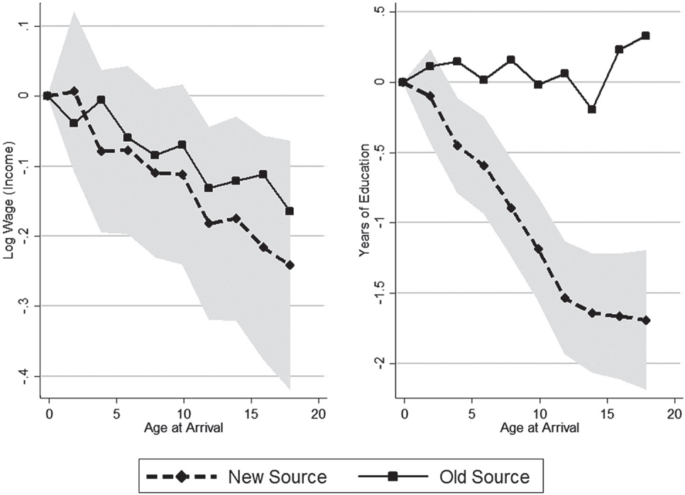
The profiles for income and education separated by New and Old sources are shown in Figure 5. On the one hand, the income profiles are similar across sources, where the negative effect of age at arrival is statistically indistinguishable across the two regions. At the same time, the education profiles were quite distinct: New sources had a steep profile where older arrivals received 1.7 fewer years of education. On the other hand, the education profile is completely flat for Old sources, showing no penalty for arriving at an older age. The flat education profile is consistent with the relatively high quality educational institutions in Northern and Western Europe.

Figure 5

The Age-At-Arrival Profiles Were Differently Sloped Across New and Old Sources

Notes: The figure shows the estimated fixed effects for age at arrival with age at arrival of zero and one being the excluded group. The shaded area is the 95 percent confidence interval for the New Source group. Standard errors are clustered at the household level. New source countries are in Southern and Western Europe and Old Source countries are in Northern and Western Europe.Sources: Linked sample of brothers from Ellis Island records to the 1940 Census.

The difference in education and income profiles across sources reveal a puzzle: why did older arrivals from Northern and Western Europe earn less despite receiving the same total years of education? One reason may be that foreign education did not yield a high return in the U.S. labor market, and thus extra schooling acquired in the source country at older ages did not boost wages. Besides education, older arrivals also had more potential labor market experience in the foreign source country, and foreign experience may not have had a high value in the United States. On the other hand, it may be that the age-at-arrival effect operated through channels other than education or experience, such as social assimilation. We now turn to other possible explanations for the effect of age at arrival.

Return to Education and Experience Separated into Domestic and Foreign Component

Since we observe age of arrival and completed years of education in our dataset, we can test—after making a few assumptions—whether foreign education and experience yielded a small return in the United States. Following Rachel Friedberg (Reference Friedberg2000), we assume that individuals entered school at age six, and then allocate the total amount of schooling to the United States or source country based on the age of arrival.Footnote ²⁶ Given this assumption, it is straightforward to further separate potential experience into foreign or U.S. components. See the descriptive statistics in Table 2 for how foreign education and experience increase at higher ages of arrival, while years of U.S. education decreases.

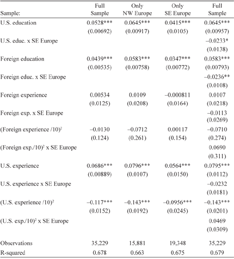
To measure the wage return to education and experience, we use an augmented Mincer equation and regress log income on years of U.S. education, years of foreign education, potential years of U.S. experience, and potential years of foreign experience:

(4) ${y_{ih}} = {\beta _0} + {\beta _1}{\rm{ }}ForEdu{c_{ih}} + {\beta _2}{\rm{ }}USEdu{c_{ih}} + f\left( {ForEx{p_{ih}}} \right) + g\left( {USEx{p_{ih}}} \right) + {\phi _h} + {\upsilon _{ih}}.$

We are interested in whether the return to foreign education was less than the return to U.S. education, that is if β ₁ < β ₂. We are also interested in whether the return to experience gained abroad yielded a different return from experience gained in the United States; we model experience as a quadratic. Note that we always include household fixed effects, eliminating household-invariant unobservables that are correlated with years of education, experience, and income.

The results are presented in Table 4. When pooling New and Old source countries together, the return to being educated in the United States is estimated at 5.3 percent, which is less than the return for native-born workers (6.5–7.9 percent). A different return to U.S. education for foreign-born workers relative to native workers has been found elsewhere in the literature (e.g., Chiswick Reference Chiswick1978; Baker and Benjamin Reference Baker and Benjamin1994), and may reflect discrimination against foreign-born workers or the quality of “years” of education. The return to education earned in the foreign country was even lower at 4.4 percent, although the 0.9 percentage point difference from the return to U.S. education is not statistically significant.

Table 4

The Return to Education and Experience Separated by United States and Foreign Component

Notes:

^*** p<0.01

^** p<0.05

^* p<0.10

The dependent variable is log wage income. We assume that individuals enter school at age six and stay in school continuously in order to separate totals years of education and potential experience into foreign and U.S. components. Brothers fixed effects are included in each column.

Sources: Linked sample of brothers from Ellis Island records to the 1940 Census.

While there is not strong evidence that the location of schooling mattered, there is evidence that where one gained labor market experience mattered. Table 4 shows that the return to potential foreign experience was not statistically distinguishable from zero, although this is not very precisely estimated, whereas U.S. experience was positively rewarded. A small return for foreign experience may reflect that immigrants entered different industries and occupations after the move to the United States. Immigrants often came from more agrarian countries in Southern and Eastern Europe, and their European experience appears to have had little value in the United States (Hatton and Williamson Reference Hatton and Williamson1998, Chapter 2). However, this is part speculation, unfortunately we cannot observe the job history of migrants to determine the value of the type of foreign experience. Data that does observe young arrivals’ occupations show that most teenagers reported holding either no job or an unskilled job.Footnote ²⁷ If skills learned in these jobs in the source country did not transfer to the U.S. labor market, then older arrivals would be penalized for staying longer in the source country.

The return to human capital may have differed between sources closer in development to the United States and sources further behind. We test for this in Columns 2 and 3 after splitting the sample into New and Old sources. The results show that the return to foreign education was indeed higher for Old sources at 6.5 percent than for New sources at 4.1 percent—a statistically significant difference, as shown in the fully interacted model in the last column. This result implies that education acquired in Northern and Western Europe more easily transferred to the United States, perhaps because it was of higher quality or the economies were closer in industrial structure. Yet at the same time, immigrants from Northern and Western Europe did not earn much return to foreign experience, and the return to foreign experience was similar across regions in Europe.

The results from these wage regressions point to foreign experience and its lack of return as a potential mechanism for a downward sloping age-at-arrival and income profile. For example, 16–20 year old arrivals had on average 5.7 years of potential foreign experience (see Table 2), but this human capital yielded little return in the U.S. labor market. This result may partially explain the result in Figure 5 that Old source immigrants had a negative age-at-arrival effect on income despite a lack of effect on education; however, other channels, such as the extent of social assimilation, may have also been important.

Social Assimilation: Intermarriage and Geography

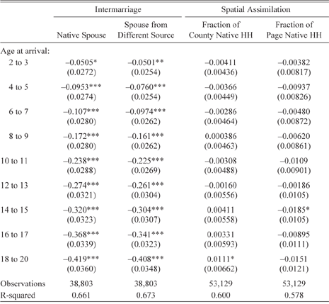
Besides the traditional measures of human capital such as education and experience, age at arrival may have affected adult earnings through a different channel: social assimilation. This could be due to higher levels of English fluency for younger arrivals or because younger arrivals appeared more “American” and thus experienced less discrimination. We measure the effect of age at arrival on social assimilation by changing the dependent variable to outcomes related to residential segregation and marriage; specifically, the likelihood of living near native-born households and the likelihood of marrying a native-born spouse.Footnote ²⁸ English fluency is not observed in the 1940 Census, but we discuss the potential effect of English fluency in the next section.

Age at arrival had a strong effect on intermarriage, as shown in Table 5. A 16-year-old arrival was 37.2 percentage points less likely to marry a native-born spouse than a one-year-old arrival, a very large effect given that 69 percent of infant arrivals married a native-born spouse. Although we do not estimate the return to intermarriage, others have shown with late-twentieth century data that intermarriage is associated with higher earnings (e.g., Meng and Gregory Reference Meng and Gregory2005); therefore, it may be a mechanism for the downward sloping age-at-arrival income profile.

Table 5

Effect of Age at Arrival on Social Outcomes

Notes:

^*** p<0.01

^** p<0.05

^* p<0.10

For the first two columns, we only include people who are married. The first column regresses whether the spouse is native-born on age at arrival, and the second column regresses whether the spouse is from a different source country on age at arrival. The fraction of page that are native household heads is the census page, which reflects immediate neighbors. Brothers fixed effects are included in each column.

Sources: Linked sample of brothers from Ellis Island records to the 1940 Census.

While there is a large effect of age at arrival on intermarriage, there is little evidence that younger arrivals were more spatially integrated with native-born household heads. Table 5 also shows the effect of age at arrival on the fraction of native-born household heads in the county of residence. Note that we use fraction of native-born household heads rather than fraction of all individuals in the county to ensure that native-born second-generation children in the home do not influence the estimate (i.e., “childrearing” bias). We find that age at arrival had no effect on living in a county with more native-born household heads. However, this county-level measure may mask segregation within a county. Given that we have the entire 1940 Census, we can further narrow the geography from county to the immediate neighborhood, as proxied by the fraction of native-born household heads on the same census page (Logan and Parman Reference Logan and Parman2017). However, even using this measure suggests that age at arrival had little impact on spatial assimilation for our dataset of brothers.

Conclusion

Using a new dataset of brothers linked from Ellis Island records to the 1940 Census, we show that there was a large wage and educational return to arriving at a younger age in the United States. Spending one’s childhood in the United States rather than in Europe significantly improved immigrants’ long-run economic outcomes. The variation in immigrant outcomes based on their age at arrival complements prior research that finds that occupational-based earning differentials between migrants and natives were fixed throughout the life cycle. The difference in results suggests that while human capital acquired during childhood led to a large occupational return, the human capital acquired during adulthood after arrival did not (Abramitzky, Boustan, and Erkisson Reference Abramitzky, Boustan and Eriksson2014; Ward Reference Ward2018).

While the results suggest that the U.S. childhood environment was advantageous relative to that of Europe, the results are limited by the lack of data on childhood location in the United States. In particular, one question that is left unanswered is the effect of childhood environment when living in or outside an ethnic enclave. Given the intergenerational literature’s result that the source country’s position in the occupational distribution persists across generations of immigrants despite our result of childhood environment having a large effect, persistence of skill levels across generations must be due to other factors such as immigrants sorting into different quality childhood environments in the United States (Abramitzky, Boustan, and Erkisson Reference Abramitzky, Boustan and Eriksson2014, Borjas Reference Borjas1994).

Finally, the results show that immigrants’ position in the skill distribution was not fixed by inherited or genetic factors, as many nativists at the time claimed. For example, Francis Walker, one-time president of the American Economic Association, charged that New source immigrants had “none of the inherited instincts and tendencies which made it comparatively easy to deal with the immigration of the olden time. They are beaten men from beaten races; representing the worst failures in the struggle for existences. Centuries are against them” (Walker Reference Walker1896). This pessimistic view of immigrants has been reprised throughout time, right up to today’s wave of nativism against Muslims and Hispanics (Higham Reference Higham1955; Huntington Reference Huntington2004). Our research shows that these “beaten men from beaten races” in the past did remarkably well with a change to their location at young ages, reaffirming the paramount importance of childhood environment for long-run outcomes.