1 Introduction
Collision of particle agglomerates with each other and with container walls or other obstacles in turbulent flow fields is important during both the agglomerate formation and breakup processes. The significance of agglomerate collisions has been studied for important industrial processes such as drug particle dispersion in dry powder inhalers (Tong et al. Reference Tong, Zheng, Yang, Yu and Chan2013, Reference Tong, Zhong, Yu, Chan and Yang2016; Yang, Wu & Adams Reference Yang, Wu and Adams2014), cyclone operation (Tong et al. Reference Tong, Yang, Chu, Yu, Adi and Chan2010) and particle filtration (Iimura et al. Reference Iimura, Suzuki, Hirota and Higashitani2009a ,Reference Iimura, Yanagiuchi, Suzuki, Hirota and Higashitani b ). Similar agglomerate–agglomerate collision processes occur in astrophysics during formation of protoplanetary disks (Ormel, Spaans & Tielens Reference Ormel, Spaans and Tielens2007; Ormel et al. Reference Ormel, Paszun, Dominik and Tielens2009) and in the dynamics of planetary rings (Schäfer, Speith & Kley Reference Schäfer, Speith and Kley2007).
The development of particle agglomerates in turbulent flows occurs through a series of processes in which individual particles collide and adhere to form small agglomerates, and these small agglomerates then collide and adhere to each other to form larger agglomerates, and so forth (Dizaji & Marshall Reference Dizaji and Marshall2016, Reference Dizaji and Marshall2017). As they increase in size, the agglomerates begin to lose particles by processes such as erosion of small groups of particles from an agglomerate surface or rupture of the agglomerate into smaller pieces in response to the fluctuating turbulent shear flow (Serra, Colomer & Casamitjana Reference Serra, Colomer and Casamitjana1997; Higashitani, Iimura & Sanda Reference Higashitani, Iimura and Sanda2001), eventually balancing the agglomerate formation processes to achieve a quasi-equilibrium state (provided that the turbulence itself is in an equilibrium state). As discussed by Sayvet & Navard (Reference Sayvet and Navard2000), a dominant agglomerate breakup process for turbulent flows at lower shear stress values is fragmentation of agglomerates during collisions with other agglomerates. The question of whether two colliding agglomerates will merge together, bounce off each other, or split apart into a larger number of fragments is thus one of central importance for a wide range of processes. All three of these outcomes were observed under different conditions in a microgravity experiment of particle agglomerates in a vibrating box by Brisset et al. (Reference Brisset, Heißelmann, Kothe, Weidling and Blum2016) for different values of the collision velocity, and in a normal gravity experiment by Ihalainen et al. (Reference Ihalainen, Lind, Torvela, Lehtinen and Jokiniemi2012) in which agglomerates were impacted onto a flat surface.
An important simplification that is often made in modelling turbulent agglomeration is replacement of a particle agglomerate by a single ‘effective particle’, often selected as a sphere with the same mass as the agglomerate. This assumption is integral to the traditional population balance model for agglomerate formation (Smoluchowski Reference Smoluchowski1917; Lu & Wang Reference Lu and Wang2006; Reinhold & Briesen Reference Reinhold and Briesen2012), and it plays an important part in many analytical statistical models for the early stages of agglomerate formation in turbulence (Brunk, Koch & Lion Reference Brunk, Koch and Lion1998; Wang, Wexler & Zhou Reference Wang, Wexler and Zhou1998; Koch & Pope Reference Koch and Pope2002; Chun & Koch Reference Chun and Koch2005). The equivalent sphere assumption is also used in the ‘extended hard-sphere’ discrete-element method (DEM), which seeks to use the hard-sphere approach for binary collisions to study the formation of particle agglomerates (Kosinski & Hoffmann Reference Kosinski and Hoffmann2010; Balakin, Hoffmann & Kosinski Reference Balakin, Hoffmann and Kosinski2011). All such applications of this equivalent sphere approximation must impose some external criterion for whether or not an agglomerate will stick or bounce upon collision. Although the equivalent sphere approximation is commonly made for simulation of turbulent flows of adhesive particles, the accuracy of this approximation has not been addressed in detail. Can mechanical properties be assigned to the effective particle such that its collision with another effective particle accurately approximates the collision of two agglomerates? Are agglomerate collisions more complex than can be represented by a simple stick or bounce decision? Addressing these questions is one of the primary objectives of the current paper.
There is a fairly large literature on use of the DEM for examining collision of tightly packed agglomerates with a wall (Ning et al. Reference Ning, Boerefijn, Ghadiri and Thornton1997; Lian, Thornton & Adams Reference Lian, Thornton and Adams1998; Thornton, Ciomocos & Adams Reference Thornton, Ciomocos and Adams1999; Kafui & Thornton Reference Kafui and Thornton2000; Moreno, Ghadiri & Antony Reference Moreno, Ghadiri and Antony2003; Thornton & Liu Reference Thornton and Liu2004; Moreno-Atanasio & Ghadiri Reference Moreno-Atanasio and Ghadiri2006), with each other (Kun & Herrmann Reference Kun and Herrmann1999; Schäfer et al. Reference Schäfer, Speith and Kley2007; Tong et al. Reference Tong, Yang, Yu, Adi and Chan2009; Seizinger & Kley Reference Seizinger and Kley2013), or with some other obstacle, such as a cylinder or sphere in the flow field (Iimura et al. Reference Iimura, Suzuki, Hirota and Higashitani2009a ,Reference Iimura, Yanagiuchi, Suzuki, Hirota and Higashitani b ; Yang et al. Reference Yang, Wu and Adams2014). Experimental studies of collisions of compressed particle aggregates with each other (Beitz et al. Reference Beitz, Güttler, Blum, Meisner, Teiser and Wurm2011) and with a wall (Samimi, Moreno & Ghadiri Reference Samimi, Moreno and Ghadiri2004) have also been reported. Much of this work is motivated by the problem of deagglomeration of particles in dry powder inhalers (Tong et al. Reference Tong, Zheng, Yang, Yu and Chan2013, Reference Tong, Zhong, Yu, Chan and Yang2016; Yang et al. Reference Yang, Wu and Adams2014), used to break up agglomerates and deliver small drug particles to the lungs, where they are absorbed. In this application, the particles are initially compressed into tightly packed aggregates at the time of manufacture, which then need to be broken up to release the small drug particles at time of use. Alternatively, ice particles can form tightly packed aggregates in planetary rings (Schäfer et al. Reference Schäfer, Speith and Kley2007), and the dynamics of their collision plays a central role in understanding the ring dynamics.
A useful definition of agglomerate strength was given by Moreno-Atanasio & Ghadiri (Reference Moreno-Atanasio and Ghadiri2006), based on the work of Rumpf (Reference Rumpf and Knepper1962), as ‘the force that is required to break all contacts simultaneously on a prescribed failure plane’. This force depends on both the strength of the individual contacts and the number of contacts in the failure plane. The number of contacts in any given cross-sectional plane increases with the agglomerate fractal dimension, with higher values for tightly packed agglomerates with fractal dimension close to
 $d_{f}\cong 3$
and lower values for the loosely structured agglomerates more typically formed in turbulent flocculation processes, with fractal dimension closer to
 $d_{f}\sim 2$
. For instance, in experiments with turbulent agglomeration of latex particles in stirred tanks, Selomulya et al. (Reference Selomulya, Amal, Bushell and Waite2001) reported
 $d_{f}$
between 1.7 and 2.1, and Waldner et al. (Reference Waldner, Sefcik, Soos and Morbidelli2005) reported
 $d_{f}$
in the range 1.8–2.6. The above definition of agglomerate strength is based on the idea of pulling an agglomerate apart in tension, whereas the agglomerate response to collision is also dependent on its behaviour under compression. In compressive deformation, agglomerates with lower values of particle concentration are more susceptible to buckling of force chains due to having fewer surrounding particles (Marangoni & Narine Reference Marangoni, Narine, Widlak, Hartel and Narine2001). The sensitivity of agglomerate collisions to particle concentration
 $c$
(or void fraction
 $\unicode[STIX]{x1D700}=1-c$
) was noted in DEM simulations by Gunkelmann, Ringl & Urbassek (Reference Gunkelmann, Ringl and Urbassek2016), who in a study of head-on collision of two agglomerates in a vacuum found that agglomerates with higher porosities are more fragile during collision and have higher tendency to fragment. These conclusions are also supported by the simulations of Nguyen et al. (Reference Nguyen, Rasmuson, Thalberg and Björn2014) of the collision of a loosely structured agglomerate of fine particles with a larger spherical particle, who found a higher tendency of the loosely structured agglomerate to fragment compared to simulations with highly packed agglomerates.
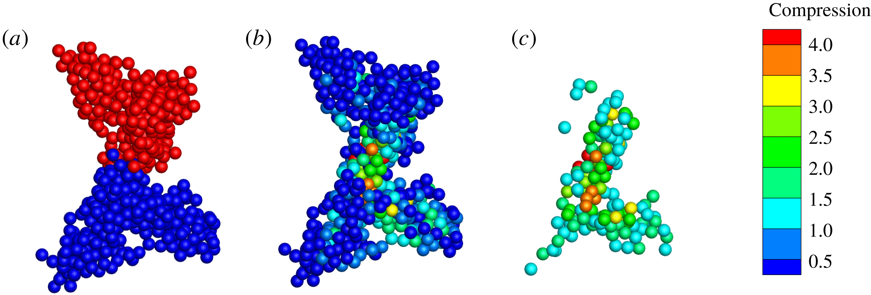
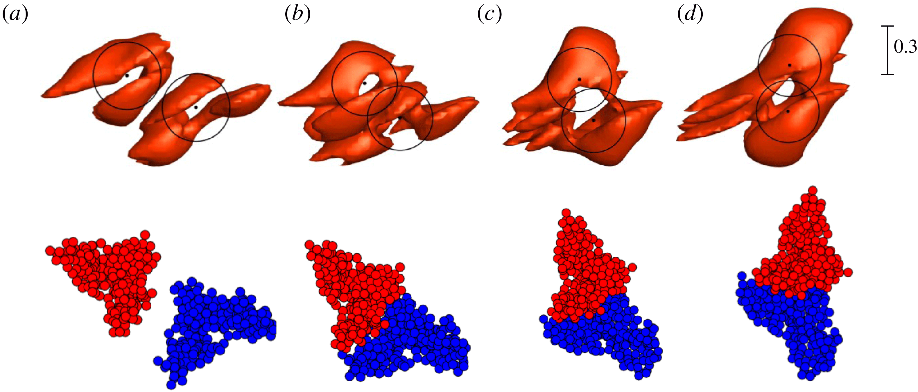
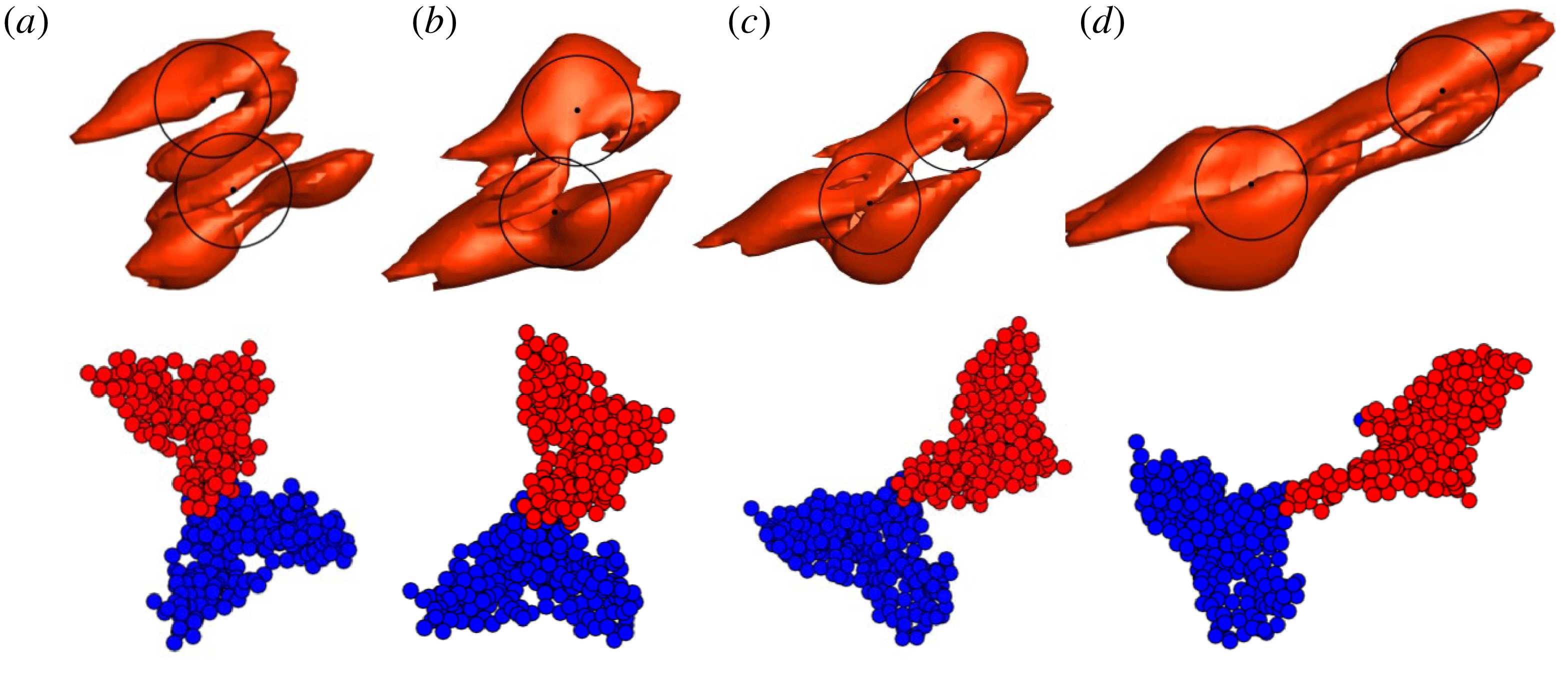
The current paper examines the collision of two particle agglomerates in a shear flow under conditions typical of agglomerate collision in turbulent flows. The primary objective of the paper is to address two issues: (1) to understand the flow field induced by a particle agglomerate in a shear flow, and (2) to evaluate the accuracy of the equivalent sphere approximation by examining the physics of actual agglomerate–agglomerate collisions with loosely structured agglomerates. The agglomerate collision is computed using a computational fluid dynamics–discrete-element method (CFD-DEM) approach based on the soft-sphere method with four-way coupling. The CFD-DEM approach does not resolve flow around individual particles, but instead it introduces a distributed body force that accounts for the influence of particles on the bulk fluid flow. The bulk flow within the agglomerates can be resolved by the fluid flow computation since the agglomerates selected consist of several hundred particles, and so are much larger than the individual particle size. Loosely structured agglomerates are first generated from a direct numerical simulation of turbulent agglomeration (Dizaji & Marshall Reference Dizaji and Marshall2016), and from which agglomerates are extracted and placed in a shear flow. We first examine agglomerate evolution and breakup in shear with no collision, and then examine the effect of two-agglomerate collision on agglomerate merger, bouncing and fragmentation. The paper differs from previous work in its focus on agglomerate collision in shear flows, in its use of loosely structured agglomerates typical of turbulent flocculation processes, and in its focus on fluid flow effects on the agglomerate collision.
2 Computational method
The agglomerate breakup and collision are computed using the four-way coupled CFD-DEM approach, using an adhesive soft-sphere DEM for the particles and a high-order finite-difference method for the fluid. The DEM approach is based on evolving the motion of each individual particle by solution of the particle momentum and angular momentum equations, while accounting for the many different forces and torques acting between the particles due to collision and van der Waals adhesion effects as well as between the particles and the surrounding fluid via a set of model equations. The flow around each individual particle is not resolved, but rather the computational method introduces the force imposed by the particles on the fluid as a smooth body force field, which is generated by the combined forces acting on many particles in a local region. A conservative particle blob method (Marshall & Sala Reference Marshall and Sala2013) is used in the current paper to translate between forces on individual particles and the body force acting on the fluid grid in a manner that is well suited for cases where the ratio of particle diameter to the grid cell spacing is of order unity.
The soft-sphere DEM formulation can be used both to simulate isolated particles and to simulate particles contained in agglomerates. An agglomerate is defined in the current paper as an assemblage of particles in which each particle in the agglomerate is in contact with at least one other particle in the agglomerate, in such a manner that one can continuously travel between any two particles in the agglomerate by following a chain of contacts. With use of the soft-sphere DEM approach, the motion and deformation of the agglomerate is simulated by evolving the motion and rotation of its constituent parts.
As is standard in DEM, the drag on each particle is given by the Stokes drag expression multiplied by a particle crowding factor that accounts for the effect of surrounding particles on the drag force and an inertia factor that accounts for finite particle inertia. The particle crowding factor was determined empirically as a function of the local particle concentration and the particle Reynolds number based on experiments with a fluidized particle bed (Di Felice Reference Di Felice1994). While this approach is commonly employed, we note that it does not account for the effects of strongly heterogeneous concentration along the sides of the agglomerate. The pairwise-interaction extended point-particle (PIEPP) method recently proposed by Akiki, Moore & Balachandar (Reference Akiki, Moore and Balachandar2017a ) and Akiki, Jackson & Balachandar (Reference Akiki, Jackson and Balachandar2017b ) might be one approach that could be used to account for the effect of heterogeneity in future studies of agglomerate flows. However, even without such corrections, previous studies with the CFD-DEM method, such as that of Bosse et al. (Reference Bosse, Kleiser, Härtel and Meiburg2005) for a particle suspension droplet falling under gravity, have produced predictions for agglomerate formation and dynamics in excellent agreement with experimental observations. A review of the CFD-DEM approach by Zhu et al. (Reference Zhu, Zhou, Yang and Yu2007) provides a detailed discussion of the modelling approximations used in this method.
The computations proceed in two parts. The first part is concerned with the initial formation of agglomerates in a turbulent flow, and the approach used for these computations has been described in detail in a previous paper (Dizaji & Marshall Reference Dizaji and Marshall2017). The second part conducts a detailed examination of the collision process that occurs when either one or two of the agglomerates are extracted and placed in a plane shear flow, which is intended to represent a very small section of the overall turbulent flow. A summary of the DEM and CFD methods used to simulate the particles and the fluid flow, and of the turbulent flow computations used to initialize the agglomerate structure, is given below.
2.1 Discrete element method
The computations of particle agglomerate breakup and collision are performed using a soft-sphere adhesive DEM (Marshall Reference Marshall2009; Marshall & Li Reference Marshall and Li2014). Because particle collision and adhesion processes involve a wide range of time scales, a multiple-time-step algorithm is used in the current paper in which the fluid time step
 $\unicode[STIX]{x0394}t=O(\ell /u_{0})$
, the particle time step
 $\unicode[STIX]{x0394}t_{p}=O(d/u_{0})$
and the collision time step
 $\unicode[STIX]{x0394}t_{c}=O(d(\unicode[STIX]{x1D70C}_{p}^{2}/E_{p}^{2}u_{0})^{1/5})$
satisfy
 $\unicode[STIX]{x0394}t>\unicode[STIX]{x0394}t_{p}>\unicode[STIX]{x0394}t_{c}$
. Here
 $d$
is the particle diameter,
 $\unicode[STIX]{x1D70C}_{p}$
is the particle density and
 $E_{p}$
is the particle elastic modulus. The method follows the motion of individual particles in the three-dimensional fluid flow by solution of the particle momentum and angular momentum equations
 $$\begin{eqnarray}m\frac{\text{d}\boldsymbol{v}}{\text{d}t}=\boldsymbol{F}_{F}+\boldsymbol{F}_{A},\quad I\frac{\text{d}\unicode[STIX]{x1D734}}{\text{d}t}=\boldsymbol{M}_{F}+\boldsymbol{M}_{A},\end{eqnarray}$$
subject to forces and torques induced by the fluid flow (
 $\boldsymbol{F}_{F}$
,
 $\boldsymbol{M}_{F}$
) and by particle collision and van der Waals adhesion (
 $\boldsymbol{F}_{A}$
,
 $\boldsymbol{M}_{A}$
). In this equation,
 $m$
is the particle mass,
 $I$
is the moment of inertia, and
 $\boldsymbol{v}$
and
 $\unicode[STIX]{x1D734}$
are the particle velocity and rotation rate, respectively. The dominant fluid force is the drag force, given by the Stokes drag law modified to account for the effects of particle inertia and local particle crowding as
 $$\begin{eqnarray}\boldsymbol{F}_{d}=3\unicode[STIX]{x03C0}\unicode[STIX]{x1D707}d(\boldsymbol{u}-\boldsymbol{v})f,\end{eqnarray}$$
where
 $\boldsymbol{u}$
is the fluid velocity evaluated at the particle centroid. The friction factor
 $f=C_{I}C_{C}$
is written as the product of an inertial correction term
 $C_{I}$
and a particle crowding correction term
 $C_{C}$
. An expression for the inertial correction was given by Schiller & Naumann (Reference Schiller and Naumann1933) as
 $$\begin{eqnarray}C_{I}=1+0.15Re_{p}^{0.687},\end{eqnarray}$$
where
 $Re_{p}=\unicode[STIX]{x1D70C}_{f}\,\text{d}v_{s}/\unicode[STIX]{x1D707}$
is the particle Reynolds number and
 $v_{s}=|\boldsymbol{v}-\boldsymbol{u}|$
is the magnitude of the particle slip velocity relative to the fluid. This expression is valid to within 5 % of comparison experimental data for particle Reynolds number up to approximately 800. An expression for the crowding correction factor was determined empirically by Di Felice (Reference Di Felice1994) for particle Reynolds numbers in the range 0.01–
 $10^{4}$
as a function of the void fraction
 $\unicode[STIX]{x1D700}$
as
 $$\begin{eqnarray}C_{C}=\unicode[STIX]{x1D700}^{1-\unicode[STIX]{x1D701}},\quad \unicode[STIX]{x1D701}=3.7-0.65\exp \left(-{\textstyle \frac{1}{2}}[1.5-\ln (Re_{p})]^{2}\right).\end{eqnarray}$$
This expression approaches the Wen & Yu (Reference Wen and Yu1966) expression for low particle Reynolds number. A viscous fluid torque arises from a difference in rotation rate of the particle and the local fluid element (Crowe et al. Reference Crowe, Schwarzkopf, Sommerfeld and Tsuji2012), and is given by
 $$\begin{eqnarray}\boldsymbol{M}_{F}=-\unicode[STIX]{x03C0}\unicode[STIX]{x1D707}d^{3}\left(\unicode[STIX]{x1D734}-{\textstyle \frac{1}{2}}\unicode[STIX]{x1D74E}\right),\end{eqnarray}$$
where
 $\unicode[STIX]{x1D74E}$
is the fluid vorticity vector. While the drag is the primary fluid force acting on the particles, we also include in the computations several secondary forces such as the added-mass force and the Saffman and Magnus lift forces (Rubinow & Keller Reference Rubinow and Keller1961; Saffman Reference Saffman1965).
Particle collision and van der Waals adhesion forces are simulated using the classical Johnson–Kendall–Roberts (JKR) theory (Johnson, Kendall & Roberts Reference Johnson, Kendall and Roberts1971). This theory assumes that particle diameter is much larger than the effective length scale over which the van der Waals adhesion force acts (approximately 10 nm), so that the adhesion force can be assumed to act only within the flattened contact region between two colliding particles. No adhesion force acts between the particles prior to or following collision, when the particles are not in contact. Since the size of the contact region depends on both the elastic and adhesive forces, these forces are nonlinearly combined to yield the total contact/adhesion force on any pair of particles in contact with each other.
The collision and adhesion force and torque fields acting on particle
 $i$
, with radius
 $r_{i}$
, are given by
 $$\begin{eqnarray}\boldsymbol{F}_{A}=F_{n}\boldsymbol{n}+F_{s}\boldsymbol{t}_{S},\quad \boldsymbol{M}_{A}=rF_{s}(\boldsymbol{n}\times \boldsymbol{t}_{S})+M_{r}(\boldsymbol{t}_{R}\times \boldsymbol{n}),\end{eqnarray}$$
where
 $\boldsymbol{n}=(\boldsymbol{x}_{j}-\boldsymbol{x}_{i})/|\boldsymbol{x}_{j}-\boldsymbol{x}_{i}|$
is the unit normal vector oriented along the line connecting the centres of the two colliding particles,
 $i$
and
 $j$
. The normal component of the collision and adhesion force
 $F_{n}$
is further divided into an elastic adhesion part
 $F_{ne}$
and a dissipative part
 $F_{nd}$
. The sliding resistance is composed of a force with magnitude
 $F_{s}$
acting in a direction
 $\boldsymbol{t}_{S}$
, corresponding to the direction of relative motion of the particle surfaces at the contact point projected onto the contact plane (the plane orthogonal to
 $\boldsymbol{n}$
), as well as a related torque in the
 $\boldsymbol{n}\times \boldsymbol{t}_{S}$
direction. The rolling resistance, which arises due to the effects of particle adhesion, exerts a torque of magnitude
 $M_{r}$
on the particle in the
 $\boldsymbol{t}_{R}\times \boldsymbol{n}$
direction, where
 $\boldsymbol{t}_{R}$
is the direction of the ‘rolling’ velocity. While all of these various collision and adhesion forces and torques are included in the current computations, the dynamics of small adhesive particles are dominated by the normal elastic adhesive force and the rolling resistance torque.
The effective elastic modulus
 $E$
and the effective radius
 $R$
are defined by
 $$\begin{eqnarray}\frac{1}{E}\equiv \frac{1-\unicode[STIX]{x1D70E}_{i}^{2}}{E_{i}}+\frac{1-\unicode[STIX]{x1D70E}_{j}^{2}}{E_{j}},\quad \frac{1}{R}\equiv \frac{1}{r_{i}}+\frac{1}{r_{j}},\end{eqnarray}$$
where
 $E_{i}$
,
 $\unicode[STIX]{x1D70E}_{i}$
and
 $r_{i}$
are the elastic modulus, Poisson ratio and radius of particle
 $i$
, respectively. The adhesive force between the two particles depends on the surface energy potential
 $\unicode[STIX]{x1D6FE}$
, where the work required to separate two spheres colliding over a contact region of radius
 $a(t)$
is given by
 $2\unicode[STIX]{x03C0}\unicode[STIX]{x1D6FE}a^{2}$
in the absence of further elastic deformation. Particle normal elastic rebound force and van der Waals adhesion force are simulated using the JKR theory, which can be written in terms of the contact region radius
 $a(t)$
and the normal particle overlap
 $\unicode[STIX]{x1D6FF}_{N}=r_{i}+r_{j}-|\boldsymbol{x}_{i}-\boldsymbol{x}_{j}|$
as (Chokshi, Tielens & Hollenbach Reference Chokshi, Tielens and Hollenbach1993)
 $$\begin{eqnarray}\frac{\unicode[STIX]{x1D6FF}_{N}}{\unicode[STIX]{x1D6FF}_{c}}=6^{1/3}\left[2\left(\frac{a}{a_{o}}\right)^{2}-\frac{4}{3}\left(\frac{a}{a_{o}}\right)^{1/2}\right],\quad \frac{F_{ne}}{F_{c}}=4\left(\frac{a}{a_{o}}\right)^{3}-4\left(\frac{a}{a_{o}}\right)^{3/2}.\end{eqnarray}$$
The critical overlap
 $\unicode[STIX]{x1D6FF}_{c}$
, the critical normal force
 $F_{c}$
and the equilibrium contact region radius
 $a_{o}$
are given by (Johnson et al.
Reference Johnson, Kendall and Roberts1971)
 $$\begin{eqnarray}F_{c}=3\unicode[STIX]{x03C0}\unicode[STIX]{x1D6FE}R,\quad \unicode[STIX]{x1D6FF}_{c}=\frac{a_{o}^{2}}{2(6)^{1/3}R},\quad a_{o}=\left(\frac{9\unicode[STIX]{x03C0}\unicode[STIX]{x1D6FE}R^{2}}{E}\right)^{1/3}.\end{eqnarray}$$
As two particles move away from each other following collision, they remain in contact until the point where
 $F_{n}=-F_{c}$
and
 $\unicode[STIX]{x1D6FF}_{N}=-\unicode[STIX]{x1D6FF}_{c}$
due to the necking of the material in the contact region. Beyond this state, any further separation leads the two particles to break apart.
The effect of lubrication forces within the fluid squeeze film within the contact region is to limit the minimum approach distance between the particles (i.e. the contact region gap size) and to reduce the particle restitution coefficient. Experimental studies of particle collisions at different Stokes numbers (e.g. Joseph et al.
Reference Joseph, Zenit, Hunt and Rosenwinkel2001) indicate that the coefficient of restitution is essentially zero when the Stokes number is less than approximately 10 due to dissipation in the squeeze film. We use the model of Tsuji, Tanaka & Ishida (Reference Tsuji, Tanaka and Ishida1992) for the dissipative part of the normal collision force
 $F_{nd}$
and set the damping parameter such that the restitution coefficient vanishes.
The second major effect of particle adhesion is to introduce a torque that resists particle rolling. For uniform-size spherical particles, the ‘rolling velocity’
 $\boldsymbol{v}_{L}$
of particle
 $i$
is given by (Bagi & Kuhn Reference Bagi and Kuhn2004)
 $$\begin{eqnarray}\boldsymbol{v}_{L}=-R(\unicode[STIX]{x1D734}_{i}-\unicode[STIX]{x1D734}_{j})\times \boldsymbol{n}.\end{eqnarray}$$
A linear expression for the rolling resistance torque
 $M_{r}$
is postulated as
 $$\begin{eqnarray}M_{r}=-k_{R}\unicode[STIX]{x1D709},\end{eqnarray}$$
where
 $\unicode[STIX]{x1D709}=(\int _{t_{0}}^{t}\boldsymbol{v}_{L}(\unicode[STIX]{x1D70F})\,\text{d}\unicode[STIX]{x1D70F})\boldsymbol{\cdot }\boldsymbol{t}_{R}$
is the rolling displacement in the direction
 $\boldsymbol{t}_{R}=\boldsymbol{v}_{L}/|\boldsymbol{v}_{L}|$
. Rolling involves an upward motion of the particle surfaces within one part of the contact region and a downward motion in the other part of the contact region. The presence of an adhesion force between the two contacting surfaces introduces a torque resisting rolling of the particles. An expression for the rolling resistance due to van der Waals adhesion was derived by Dominik & Tielens (Reference Dominik and Tielens1995), which yields the coefficient
 $k_{R}$
as
 $$\begin{eqnarray}k_{R}=4F_{c}(a/a_{0})^{3/2}.\end{eqnarray}$$
Dominik & Tielens (Reference Dominik and Tielens1995) further argue that the critical resistance occurs when the rolling displacement
 $\unicode[STIX]{x1D709}$
achieves a critical value, corresponding to a critical rolling angle
 $\unicode[STIX]{x1D703}_{crit}=\unicode[STIX]{x1D709}_{crit}/R$
. For
 $\unicode[STIX]{x1D703}>\unicode[STIX]{x1D703}_{crit}$
, the rolling displacement
 $\unicode[STIX]{x1D709}$
in (2.11) is replaced by
 $\unicode[STIX]{x1D709}_{crit}$
. Data for critical rolling angle for particles having diameter of approximately
 $10~\unicode[STIX]{x03BC}\text{m}$
were reported by Ding, Zhang & Cetinkaya (Reference Ding, Zhang and Cetinkaya2008), who found critical rolling angles
 $\unicode[STIX]{x1D703}_{crit}$
of between 0.02 and 0.06 rad.
A simplified expression for the effect of van der Waals adhesion on tangential sliding resistance was proposed by Thornton (Reference Thornton1991). In this model, the sliding resistance force
 $F_{s}$
is given by a spring-like expression of the form (Cleary, Metcalfe & Liffman Reference Cleary, Metcalfe and Liffman1998)
 $$\begin{eqnarray}F_{s}=-k_{T}\left(\int _{t_{0}}^{t}\boldsymbol{v}_{S}(\unicode[STIX]{x1D709})\,\text{d}\unicode[STIX]{x1D709}\right)\boldsymbol{\cdot }\boldsymbol{t}_{S}\end{eqnarray}$$
when
 $F_{s}$
is less than a critical value
 $F_{crit}$
. In (2.13), the sliding velocity
 $\boldsymbol{v}_{S}(t)$
is the relative tangential surface velocity of the particles at the contact point projection. The tangential stiffness coefficient
 $k_{T}$
was derived by Mindlin (Reference Mindlin1949) and can be written in terms of the contact region radius
 $a(t)$
as
 $$\begin{eqnarray}k_{T}=8Ga(t),\end{eqnarray}$$
where
 $G=[(2-\unicode[STIX]{x1D70E}_{i})/G_{i}+(2-\unicode[STIX]{x1D70E}_{j})/G_{j}]^{-1}$
is the effective shear modulus and
 $G_{i}\equiv E_{i}/2(1+\unicode[STIX]{x1D70E}_{j})$
. The critical sliding force is approximated using the expression
 $$\begin{eqnarray}F_{crit}=\unicode[STIX]{x1D707}_{f}|F_{ne}+2F_{c}|,\end{eqnarray}$$
where
 $F_{c}$
is the critical force for pull-off given in (2.9) and
 $\unicode[STIX]{x1D707}_{f}$
is the friction coefficient. The expression (2.15) was shown by Thornton (Reference Thornton1991) to provide results in reasonable agreement to experiments. For
 $|F_{s}|\geqslant F_{crit}$
, the sliding resistance is given by the Amonton expression
 $F_{s}=-F_{crit}$
.
2.2 Agglomerate formation
The agglomerates are formed using a turbulent agglomeration process similar to that described by Dizaji & Marshall (Reference Dizaji and Marshall2017). The computations employed a pseudo-spectral method for forced turbulence in a triply periodic domain with side length
 $2\unicode[STIX]{x03C0}$
and with 128 grid points in each direction. The turbulence is initiated with random perturbations and allowed to develop with no particles until it approached a quasi-steady state corresponding to microscale Reynolds number
 $Re_{\unicode[STIX]{x1D706}}=u_{0}\unicode[STIX]{x1D706}/\unicode[STIX]{x1D708}=99$
. Particles are then added to the computation, with 46 656 particles spread randomly over the flow field with diameter
 $d=0.04$
and particle/fluid density ratio
 $\unicode[STIX]{x1D70C}_{p}/\unicode[STIX]{x1D70C}_{f}=10$
. Over time, as the particles are advected by the flow, small agglomerates form and then collide with each other to form progressively larger agglomerates.
The computation was stopped once the agglomerates achieved a broad range of sizes. One common way to measure the size of an agglomerate is the radius of gyration
 $R_{g}$
, which for an agglomerate with
 $N$
particles is defined by
 $$\begin{eqnarray}R_{g}=\left[\mathop{\sum }_{i=1}^{N}|\boldsymbol{x}_{i}-\bar{\boldsymbol{x}}|^{2}\right]^{1/2}.\end{eqnarray}$$
In this equation,
 $\bar{\boldsymbol{x}}$
denotes the position vector of the agglomerate centroid and
 $\boldsymbol{x}_{i}$
is the centroid of the
 $i$
th particle within the agglomerate. Particle agglomerates admit a power law relating
 $N$
and
 $R_{g}$
given by (Adachi & Ooi Reference Adachi and Ooi1990)
 $$\begin{eqnarray}N=K(R_{g}/r_{p})^{d_{f}},\end{eqnarray}$$
where
 $K$
is a coefficient (called the fractal prefactor),
 $r_{p}$
is the individual particle radius, and the exponent
 $d_{f}$
is the fractal dimension of the agglomerate. The value of
 $d_{f}$
for particle agglomerates varies over the interval
 $1\leqslant d_{f}\leqslant 3$
depending on the agglomeration formation mechanism (Brasil et al.
Reference Brasil, Farias, Carvalho and Koylu2001); however, typical values for turbulent particle agglomeration processes are between approximately 1.7 and 2.8 (Selomulya et al.
Reference Selomulya, Amal, Bushell and Waite2001; Waldner et al.
Reference Waldner, Sefcik, Soos and Morbidelli2005). A log–log plot of
 $N$
versus
 $R_{g}/r_{p}$
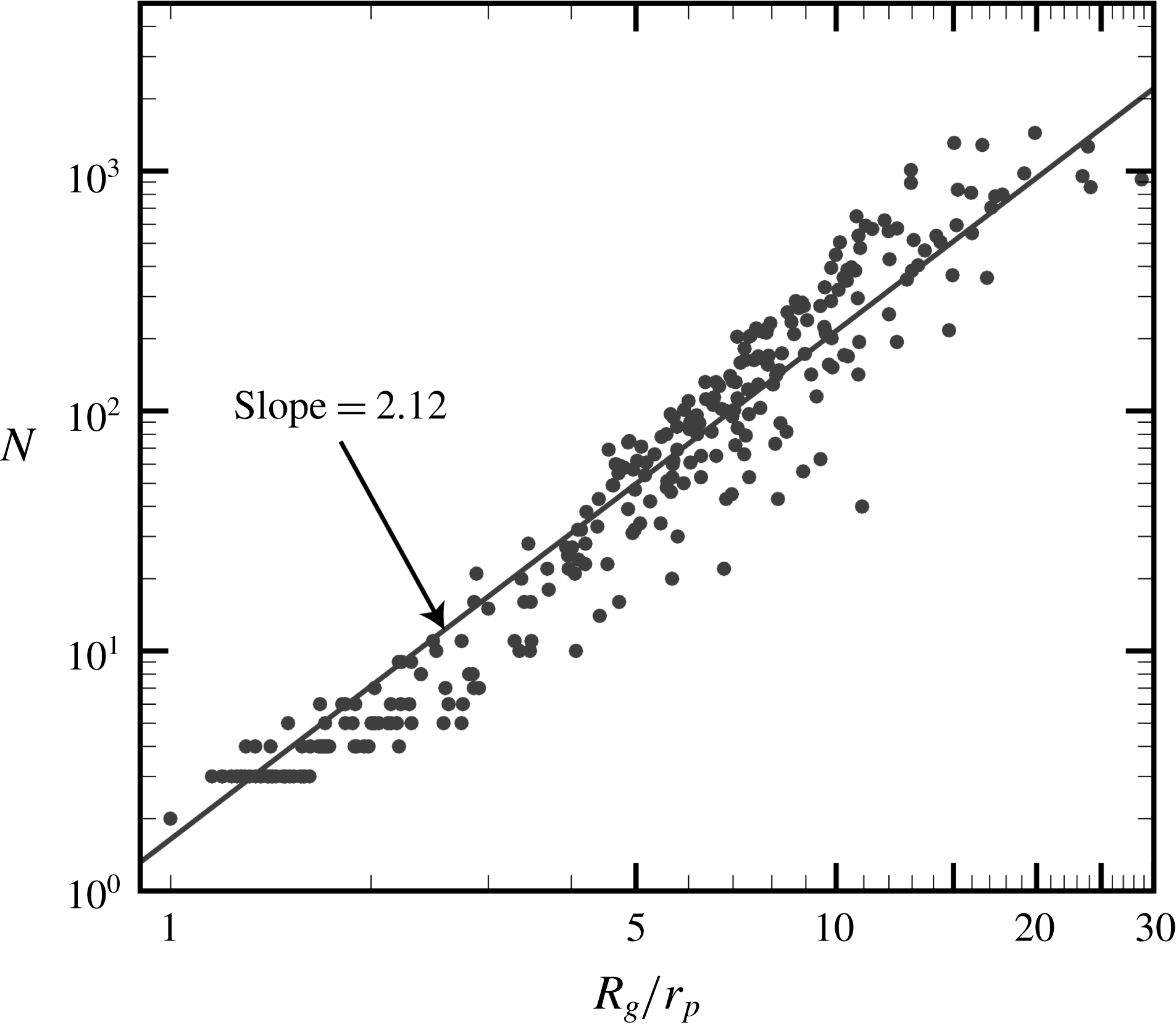
for the current turbulent flow simulation is given in figure 1. The best-fit line to the computational predictions has slope
 $d_{f}=2.12$
, which is consistent with the range of fractal dimension observed in the experimental turbulent particle agglomeration studies listed above.
Plot of the number of particles in an agglomerate
 $N$
versus the ratio of the radius of gyration of the agglomerate
 $R_{g}$
and the individual particle radius
 $r_{p}$
. The slope of the plot indicates the fractal dimension
 $d_{f}=2.12$
of the power law in (2.17).

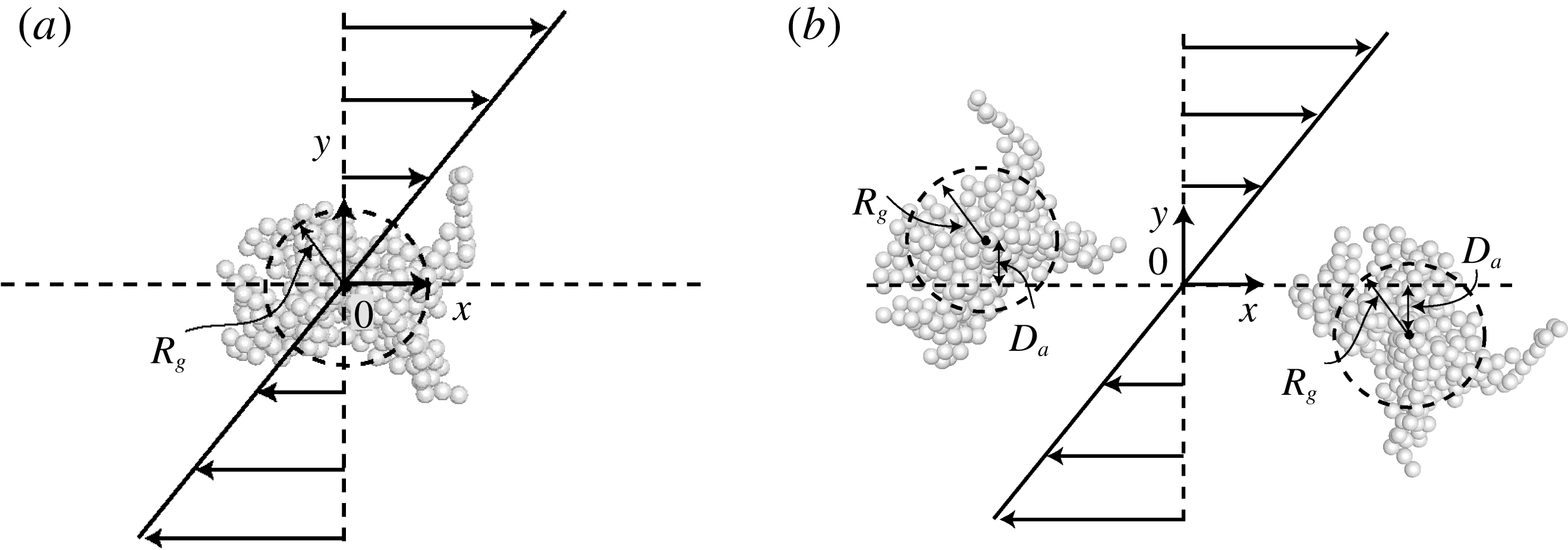
Schematic diagram of the initial conditions for the problems of (a) a single agglomerate in a shear flow and (b) two-agglomerate collision in a shear flow. Dashed circles indicate the radius of gyration
 $R_{g}$
, and the offset distance
 $D_{a}$
is indicated in (b) in both positive and negative directions.

2.3 Shear flow simulation
The agglomerates extracted from the turbulent agglomeration calculation described in § 2.2 are immersed in a linear shear flow, where the initial configuration appears as shown in figure 2(a) for cases with a single agglomerate in the shear flow and as shown in figure 2(b) for cases with agglomerate collision. Over time, the shear flow is modified by the presence of the particles, as described below. The fluid flow is assumed to be incompressible and is governed by the continuity and momentum equations of the form
 $$\begin{eqnarray}\displaystyle & \displaystyle \unicode[STIX]{x1D735}\boldsymbol{\cdot }\boldsymbol{u}=0, & \displaystyle\end{eqnarray}$$
 $$\begin{eqnarray}\displaystyle & \displaystyle \frac{\unicode[STIX]{x2202}\boldsymbol{u}}{\unicode[STIX]{x2202}t}+(\boldsymbol{u}\boldsymbol{\cdot }\unicode[STIX]{x1D735})\boldsymbol{u}=-\frac{1}{\unicode[STIX]{x1D70C}_{f}}\unicode[STIX]{x1D735}p+\unicode[STIX]{x1D708}\unicode[STIX]{x1D6FB}^{2}\boldsymbol{u}+\boldsymbol{F}_{p}. & \displaystyle\end{eqnarray}$$
 $\boldsymbol{u}$
,
 $p$
and
 $\boldsymbol{F}_{p}$
are the fluid velocity, the pressure and the particle-induced body force per unit mass, respectively. The void fraction
 $\unicode[STIX]{x1D700}=1-c$
was not included in (2.18) since our computations indicate that local void fraction remains above 90 % even within the agglomerates for the current computations due to the loose structuring of agglomerates typical of turbulent flow.
Since the grid cell size is of the same order as the particle size in these computations, we have not used the standard point-force approach in which the force imposed on the fluid by a particle is assigned to the grid cell containing the particle centre. Instead, in computing both the particle-induced body force and the particle concentration field, we have smoothed the particle field with use of the conservative particle blob method proposed by Marshall & Sala (Reference Marshall and Sala2013). In this method, the particle body force field
 $\boldsymbol{F}_{p}(\boldsymbol{x},t)$
is written as the sum of some number
 $N$
particle ‘blobs’, centred at positions
 $\boldsymbol{x}_{n}$
, as
 $$\begin{eqnarray}\boldsymbol{F}_{p}(\boldsymbol{x},t)=\mathop{\sum }_{n=1}^{N}\boldsymbol{A}_{n}f_{w}(\boldsymbol{x}-\boldsymbol{x}_{n},R_{n}).\end{eqnarray}$$
The Gaussian weight
 $f_{w}$
is a function of position and of the characteristic blob ‘radius’
 $R_{n}$
, and can be written as
 $$\begin{eqnarray}f_{w}(\boldsymbol{x}-\boldsymbol{x}_{n},R_{n})=\frac{2}{3\unicode[STIX]{x03C0}R_{n}^{3}}\exp [-|\boldsymbol{x}-\boldsymbol{x}_{n}|^{2}/R_{n}^{2}].\end{eqnarray}$$
The blob amplitude,
 $\boldsymbol{A}_{n}$
, is given by
 $$\begin{eqnarray}\boldsymbol{A}_{n}=\frac{(-\boldsymbol{F}_{f,n})}{G_{cell}\displaystyle \mathop{\sum }_{j=1}^{Q}f_{w}(\boldsymbol{g}_{j}-\boldsymbol{x}_{n},R_{n})},\end{eqnarray}$$
where
 $\boldsymbol{g}_{j}$
is the location of the centroid of grid cell
 $j$
,
 $\boldsymbol{x}_{n}$
is the centroid of particle
 $n$
,
 $G_{cell}$
is the grid cell volume, and
 $\boldsymbol{F}_{f,n}$
is the fluid-induced force acting on particle
 $n$
(which imposes an equal and opposite force
 $-\boldsymbol{F}_{f,n}$
back on the fluid). The force
 $\boldsymbol{F}_{f,n}$
is given by the sum of the drag force in (2.2) plus minor forces such as lift, added-mass force and pressure gradient force. Each particle distributes part of its force to a set
 $Q$
of surrounding grid cells, and the sum in the denominator of (2.21) is evaluated over all grid cells in this set
 $Q$
. With the choice (2.21) for blob amplitude, the discrete-to-continuum homogenization operation is discretely conservative. This method can be applied to the particle concentration simply by replacing the particle force with the particle volume.
The fluid flow computations were performed using a fractional-step method (Rai & Moin Reference Rai and Moin1991; Verzicco & Orlandi Reference Verzicco and Orlandi1996; Uhlmann Reference Uhlmann2005), with time advancement performed using the third-order Runge–Kutta method for convective terms and the second-order Crank–Nicolson method for viscous terms. Algorithms for all spatial derivatives, except the convective terms, are approximated using second-order centred finite differences (three-point stencil) on a non-staggered grid. The discretized equations for the
 $k$
th Runge–Kutta step are given by
 $$\begin{eqnarray}\displaystyle \tilde{\boldsymbol{u}} & = & \displaystyle \boldsymbol{u}^{k-1}+\unicode[STIX]{x0394}t(2\unicode[STIX]{x1D6FC}_{k}\unicode[STIX]{x1D708}\unicode[STIX]{x1D6FB}^{2}\boldsymbol{u}^{k-1}-2\unicode[STIX]{x1D6FC}_{k}\unicode[STIX]{x1D735}p^{k-1})\nonumber\\ \displaystyle & & \displaystyle -\,\unicode[STIX]{x0394}t\{\unicode[STIX]{x1D6FE}_{k}[(\boldsymbol{u}\boldsymbol{\cdot }\unicode[STIX]{x1D735})\boldsymbol{u}-\boldsymbol{F}_{p}]^{k-1}+\unicode[STIX]{x1D701}_{k}[(\boldsymbol{u}\boldsymbol{\cdot }\unicode[STIX]{x1D735})\boldsymbol{u}-\boldsymbol{F}_{p}]^{k-2}\},\qquad\end{eqnarray}$$
 $$\begin{eqnarray}\displaystyle \unicode[STIX]{x1D6FB}^{2}\boldsymbol{u}^{\ast }-\frac{\boldsymbol{u}^{\ast }}{\unicode[STIX]{x1D6FC}_{k}\unicode[STIX]{x1D708}\unicode[STIX]{x0394}t} & = & \displaystyle -\frac{\tilde{\boldsymbol{u}}}{\unicode[STIX]{x1D6FC}_{k}\unicode[STIX]{x1D708}\unicode[STIX]{x0394}t}+\unicode[STIX]{x1D6FB}^{2}\boldsymbol{u}^{k-1},\end{eqnarray}$$
 $$\begin{eqnarray}\displaystyle \unicode[STIX]{x1D735}\boldsymbol{\cdot }(\unicode[STIX]{x1D735}\unicode[STIX]{x1D719}^{k}) & = & \displaystyle \frac{\unicode[STIX]{x1D735}\boldsymbol{\cdot }\boldsymbol{u}^{\ast }}{2\unicode[STIX]{x1D6FC}_{k}\unicode[STIX]{x0394}t},\end{eqnarray}$$
 $$\begin{eqnarray}\displaystyle \boldsymbol{u}^{k} & = & \displaystyle \boldsymbol{u}^{\ast }-2\unicode[STIX]{x1D6FC}_{k}\unicode[STIX]{x0394}t\unicode[STIX]{x1D735}\unicode[STIX]{x1D719}^{k},\end{eqnarray}$$
 $$\begin{eqnarray}\displaystyle p^{k} & = & \displaystyle p^{k-1}+\unicode[STIX]{x1D719}^{k}-\unicode[STIX]{x1D6FC}_{k}\unicode[STIX]{x1D708}\unicode[STIX]{x0394}t\unicode[STIX]{x1D6FB}^{2}\unicode[STIX]{x1D719}^{k},\end{eqnarray}$$
 $\unicode[STIX]{x1D6FC}_{k}$
,
 $\unicode[STIX]{x1D6FE}_{k}$
and
 $\unicode[STIX]{x1D701}_{k}$
are coefficients given by Rai & Moin (Reference Rai and Moin1991). Continuity is enforced by a projection method leading to (2.22c
) for the pseudo-pressure, denoted by
 $\unicode[STIX]{x1D719}$
. In the multigrid solution of this equation, the five-point stencil produced by successive application of the gradient operation followed by the divergence operation was employed, rather than the finite-difference approximation to the Laplacian. The Crank–Nicolson method was used to solve the Helmholtz problem, given in (2.22b
). A tenth-order approximation was used for the convective terms, requiring an 11-point stencil. To control nonlinear instabilities, at the end of each time step the velocity components were filtered using a tenth-order filter (again using an 11-point stencil) (Lele Reference Lele1992; Steijl Reference Steijl2001). After filtering to obtain
 $\boldsymbol{u}^{filtered}$
, the velocity
 $\boldsymbol{u}$
was replaced by
 $(1-q)\boldsymbol{u}+q\boldsymbol{u}^{filtered}$
, with
 $q=0.05$
.
The flow was initialized in the
 $x$
-direction with linear variation in the
 $y$
-direction. The upper wall at
 $y=2$
was maintained at a velocity
 $u=1$
and the lower wall at
 $y=-2$
was maintained at a velocity of
 $u=-1$
, giving a dimensionless shear rate of
 $S=0.5$
. The no-slip boundary condition was applied at both the top and bottom walls in the
 $y$
-direction, and the flow was assumed to be periodic in the
 $x$
- and
 $z$
-directions. A layer of five ghost points in each direction surrounded the computational domain, so that no adjustment of the differentiation schemes was needed near the domain boundaries. The velocity on the ghost points was set at the upper and lower edges of the grid by linearly extrapolating the velocity from the point on the wall and the first point off the wall. The velocity on the ghost points in the
 $x$
- and
 $z$
-directions were set so as to enforce periodicity. The fluid flow calculations were carried out on a Cartesian grid with equal spacing in each direction. The computations were performed on a
 $128^{3}$
grid covering the interval
 $(-2,2)$
in each coordinate direction. The time step was held fixed at
 $\unicode[STIX]{x0394}t=0.005$
. The dimensionless fluid kinematic viscosity was set to
 $\unicode[STIX]{x1D708}=0.0003$
for all computations.
3 Agglomerate motion and breakup in shear flow
In this section we examine the dynamics of a single particle agglomerate exposed to shear flow, with particular focus on examination of the particle-induced flow field associated with rotation of the agglomerate in the shear flow and on the conditions for agglomerate breakup. This section helps to set the stage for the study of agglomerate collision in shear flow in the next section. The problem of agglomerate dynamics in a shear flow has been previously examined by a number of authors. A series of experiments on this problem were reported by Sonntag & Russel (Reference Sonntag and Russel1986), who found that the average radius of gyration of the agglomerates could be expressed as a power-law function of the shear rate as
 $R_{g}^{3}\propto S^{-1.06}$
. Since the average number of particles in the agglomerate,
 $N$
, was related to radius of gyration by a power-law expression of the form (2.17), with
 $d_{f}\cong 2.48$
, in their experiments, their expression for agglomerate size in the shear flow could alternatively be expressed as
 $N\propto S^{-0.878}$
.
A number of DEM simulations of agglomerate dynamics in a shear flow have been reported (Potanin Reference Potanin1993; Higashitani et al.
Reference Higashitani, Iimura and Sanda2001; Fanelli, Feke & Manas-Zloczower Reference Fanelli, Feke and Manas-Zloczower2006; Becker et al.
Reference Becker, Schlauch, Behr and Briesen2009) based on the so-called free-draining approximation, which assumes that the particles do not influence the fluid flow (one-way coupling). Potanin (Reference Potanin1993) and Becker et al. (Reference Becker, Schlauch, Behr and Briesen2009) further assumed that particles did not influence fluid forces on each other (even under close packing in the agglomerate), whereas Higashitani et al. (Reference Higashitani, Iimura and Sanda2001) and Fanelli et al. (Reference Fanelli, Feke and Manas-Zloczower2006) assumed that fluid drag forces act only on particle surfaces on the outside of the agglomerate (i.e. that fluid does not penetrate into the agglomerate). Higashitani et al. (Reference Higashitani, Iimura and Sanda2001) observed that the average number of particles in broken agglomerate fragments,
 $N$
, varies with the adhesion parameter as
 $N\propto Ad^{0.872}$
, where
 $Ad$
represents a ratio of adhesive to hydrodynamic force. Since
 $Ad$
is inversely proportional to shear rate, this observation is consistent with the scaling found experimentally by Sonntag & Russel (Reference Sonntag and Russel1986). Becker et al. (Reference Becker, Schlauch, Behr and Briesen2009) compared the DEM simulations using the free-draining approximation to a full finite-element simulation of the flow field and found that the free-draining approximation breaks down as the agglomerate size increases. This observation is consistent with that made in a recent CFD-DEM study of turbulent agglomeration by Dizaji & Marshall (Reference Dizaji and Marshall2017), who compared results with one-way and two-way coupling and found significant deviation between the two as the agglomerate size increased. Becker et al. (Reference Becker, Schlauch, Behr and Briesen2009) observed that small agglomerates rotate in an almost rigid-body fashion in the shear flow, large agglomerates break up into pieces, and agglomerates of an intermediate size undergo a restructuring process, in which they deform and change form as they rotate but do not break up.
A full CFD-DEM study of agglomerate dynamics in a shear flow was reported by Zeidan et al. (Reference Zeidan, Xu, Jia and Williams2007), but the computations were restricted to two dimensions and the models used for particle collision and adhesion forces were highly simplified. For instance, no tangential forces on the particles were included to resist rolling and sliding motions, which as noted by Becker et al. (Reference Becker, Schlauch, Behr and Briesen2009) are important in modelling agglomerate deformation under the shear flow.
In the current section, we report on a three-dimensional CFD-DEM study of agglomerate dynamics in a shear flow using a complete and well-validated DEM approach, with a focus on resolving and understanding the flow field induced by the particles. In order to work with agglomerate structures typical of those found in turbulent agglomeration processes, the computations were initiated by extracting an agglomerate from the turbulent flow computation described in § 2.2 and inserting it into an initially linear shear flow. The flow evolution is then computed using the CFD method described in § 2.3 and the DEM model described in § 2.1.
The shear flow acts to rotate and stretch the agglomerate, whereas the adhesion force acts to hold the agglomerate together as a rigid body. The competition between these two effects determines the agglomerate behaviour in the shear flow. We let
 $R_{g0}$
denote the initial radius of gyration of the agglomerate and
 $S$
denote the ambient shear rate. The characteristic length, time and velocity scales of the flow were selected as
 $R_{g0}$
,
 $1/S$
and
 $SR_{g0}$
, respectively. The primary dimensionless parameter governing the agglomerate behaviour in the shear flow is the adhesion parameter, which for current purposes is defined as the ratio of the adhesion force between individual particles (
 $O(\unicode[STIX]{x1D6FE}d)$
) to the viscous force (
 $O(\unicode[STIX]{x1D707}dU)$
) imposed on a particle by the fluid flow. Using
 $U\sim SR_{g0}$
as the typical velocity scale, the adhesion parameter for this problem takes the form
 $$\begin{eqnarray}Ad=\frac{\unicode[STIX]{x1D6FE}}{\unicode[STIX]{x1D707}SR_{g0}}.\end{eqnarray}$$
This measure is essentially the same as the inverse of the fragmentation number proposed by Hansen, Khakhars & Ottino (Reference Hansen, Khakhars and Ottino1998). A secondary parameter characterizing the particle motion is the particle Stokes number
 $St$
, which is interpreted as the ratio of particle characteristic time scale
 $\unicode[STIX]{x1D70F}_{p}=m/3\unicode[STIX]{x03C0}\unicode[STIX]{x1D707}d$
to the fluid time scale
 $\unicode[STIX]{x1D70F}_{f}=1/S$
, giving
 $$\begin{eqnarray}St=\frac{\unicode[STIX]{x1D70C}_{p}d^{2}S}{18\unicode[STIX]{x1D707}}.\end{eqnarray}$$
The values of the adhesion parameter
 $Ad$
, the initial number of particles
 $N_{0}$
, and the ratio
 $R_{g0}/d$
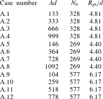
of initial agglomerate gyration radius to particle diameter are given for all single-agglomerate runs in table 1. All computations reported in the paper have Stokes number of
 $St=1.4$
and density ratio of
 $\unicode[STIX]{x1D70C}_{p}/\unicode[STIX]{x1D70C}_{f}=10$
. The shear Reynolds number can be defined in terms of shear rate and radius of gyration as
 $Re_{S}=SR_{g0}^{2}/\unicode[STIX]{x1D708}$
, which is found to have a value ranging from 52 to 102 in the current computations, depending on which of the three extracted agglomerates are under consideration. In a turbulent flow, the parameters used in these computations would therefore be larger than the Kolmogorov scale and smaller than the integral scale, perhaps typical of the Taylor microscale of the turbulent motion.
Listing of parameter values for cases examined with a single agglomerate in a shear flow, including adhesion parameter, initial number of particles, and ratio of initial gyration radius to particle diameter. For all cases examined,
 $St=1.4$
and
 $\unicode[STIX]{x1D70C}_{p}/\unicode[STIX]{x1D70C}_{f}=10$
.

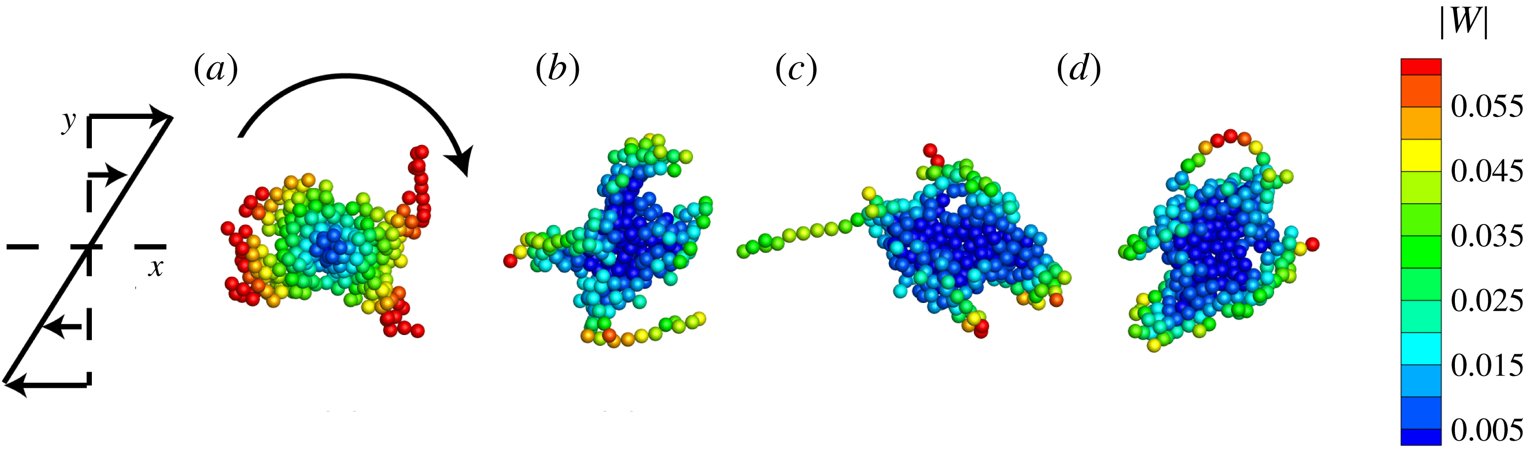
Computations in this section were performed using three different agglomerates selected from the turbulent agglomeration simulation, and for four different adhesion parameter values for each agglomerate. A time series of the particle positions during a typical run (case A.4) for a case where the agglomerate rotates without breakup, but exhibits some restructuring during the rotation, is shown in figure 3. The particles are immersed in a fluid flow, for which a velocity can be defined both outside and inside the particle agglomerate. The particles in figure 3 are coloured by the magnitude of the particle velocity relative to the fluid, which is called the relative particle velocity and defined by
 $\boldsymbol{w}\equiv \boldsymbol{v}-\boldsymbol{u}$
, where
 $\boldsymbol{v}$
and
 $\boldsymbol{u}$
denote the particle velocity and fluid velocity at the particle centroid, respectively. We will also later refer to the relative fluid velocity
 $\boldsymbol{u}_{rel}=\boldsymbol{u}-Sy\boldsymbol{e}_{x}$
, which is set equal to the computed fluid velocity
 $\boldsymbol{u}$
minus the velocity of the ambient shear flow (
 $Sy\boldsymbol{e}_{x}$
).
Particle positions at times (a)
 $t=0$
, (b) 10, (c) 20 and (d) 30 for case A.4. The particles are coloured by the magnitude of the relative velocity vector. The agglomerate is rotating clockwise in the shear flow and completes approximately one rotation in the time interval shown.

Plot showing the time variation of the gyration radius
 $R_{g}$
(solid line, left-hand axis) and the particle concentration within the agglomerate
 $c_{agg}$
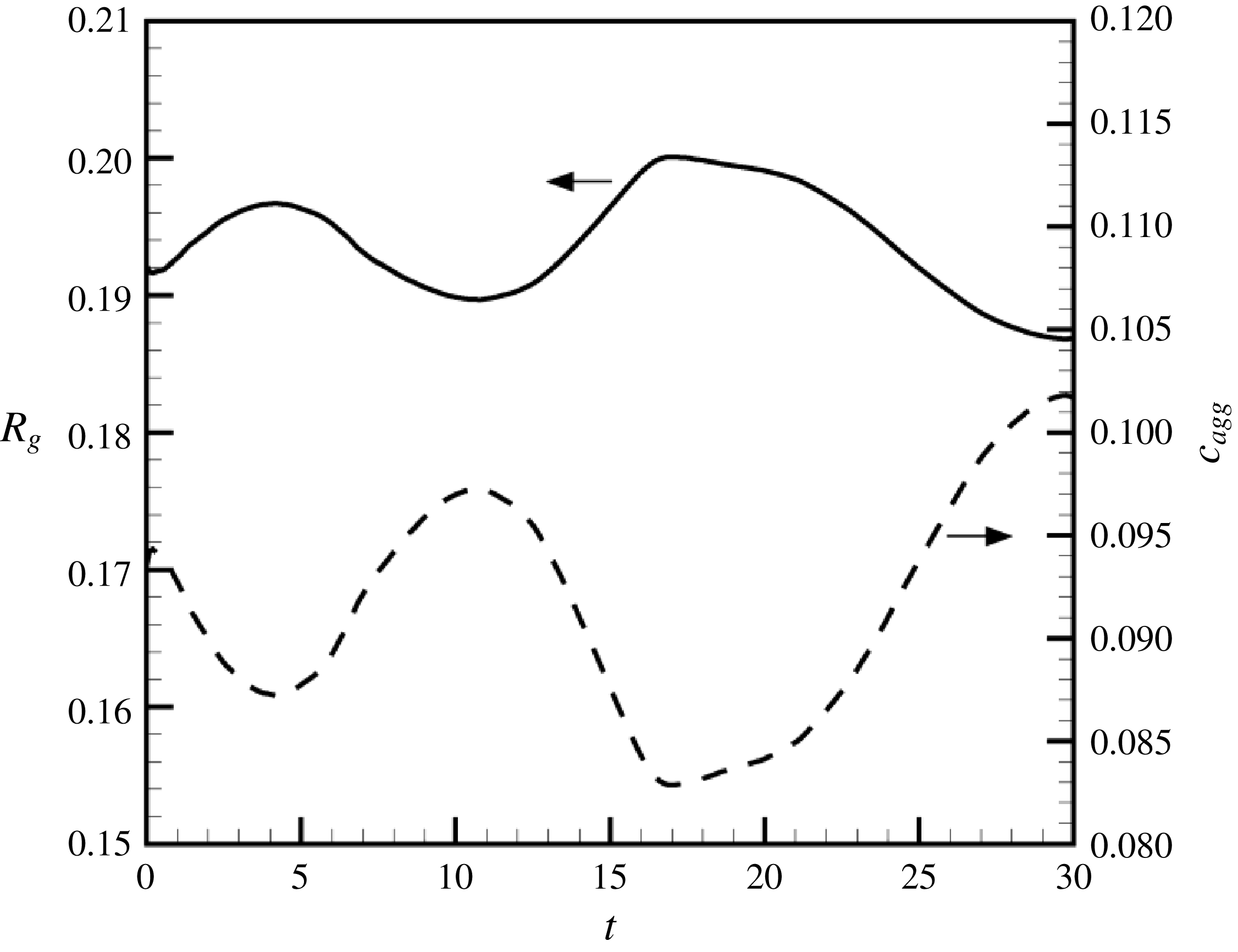
(dashed line, right-hand axis) for case A.4.

In the reported computations, the initial velocity of the fluid was set equal to the shear flow velocity
 $Sy\boldsymbol{e}_{x}$
. The initial velocity of the agglomerate particles is set equal to a rigid-body rotation at the rotation rate
 $S/2$
of the shear flow, for which there exists a vertical
 $y$
-component of velocity in addition to the
 $x$
-component of velocity characteristic of the ambient shear. This initial rotation rate of the agglomerate gives rise to a linear variation of the relative particle velocity extending outwards from the agglomerate centre, as shown in figure 3(a). At later times, the size of the region of low relative particle velocity near the agglomerate centre appears to grow and the particles with higher values of relative particle velocity are restricted to the outer parts of the agglomerate.
In the following, we shall examine in detail the results for case A.4, which is typical of a case where the agglomerate does not break up in the shear flow. The particle coordination number for this computation remains nearly constant with time at a value of 3.9. The radius of gyration
 $R_{g}$
and the particle concentration
 $c_{agg}$
within the agglomerate oscillate in time, as shown in figure 4(b). The value of
 $c_{agg}$
is computed by dividing the volume of all particles associated with the agglomerate,
 $V_{p}=(\unicode[STIX]{x03C0}/6)Nd^{3}$
, by the effective volume
 $V_{eff}$
occupied by the agglomerate. The agglomerate effective volume is estimated by
 $V_{eff}=(4\unicode[STIX]{x03C0}/3)R_{eff,i}^{3}$
, where the effective radius of the agglomerate
 $R_{eff}$
is related to the radius of gyration by
 $R_{eff}=\sqrt{5/2}R_{g}$
. This expression is based on the expression for the radius of gyration of a solid sphere of uniform density. The particle volume fraction of the agglomerate can be related to the fractal dimension by (Jiang & Logan Reference Jiang and Logan1991; Kusters, Wijers & Thoenes Reference Kusters, Wijers and Thoenes1997)
 $$\begin{eqnarray}c_{agg,i}=c_{0}(R_{g,i}/d)^{d_{f}-3},\end{eqnarray}$$
where
 $c_{0}$
is a constant. If the fractal dimension
 $d_{f}<3$
, an increase in agglomerate size results in a decrease in average particle volume fraction (Olfert, Symonds & Collings Reference Olfert, Symonds and Collings2007). Both the radius of gyration and the particle concentration
 $c_{agg}$
within the agglomerate oscillate during the computation as agglomerate restructuring occurs, with oscillation amplitude of approximately 3 % of the mean radius of gyration and 9 % of the mean particle concentration.
The time variation of the magnitude of the particle velocity
 $\boldsymbol{v}$
and the relative particle velocity
 $\boldsymbol{w}$
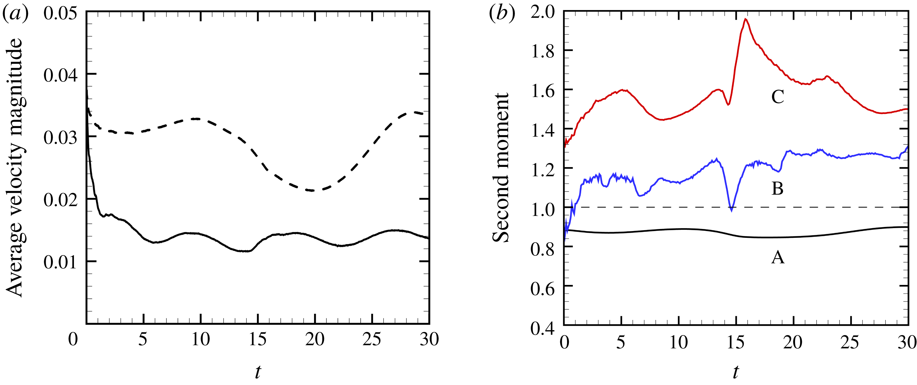
are plotted in figure 5(a). The particle velocity magnitude oscillates during the computation and the relative particle velocity exhibits a rapid initial decrease and then oscillates during the remainder of the computation. The latter result indicates that the fluid flow within the agglomerate responds quickly to changes in the particle velocity. While the relative velocity changes quickly in the time interval
 $0<t<1$
, we do not observe significant deformation or breakup of the agglomerate during this interval. The fact that the relative particle velocity magnitude is lower than the particle velocity magnitude for most of the computation is a result of the particle-induced flow, which acts to decrease the relative velocity.
Plot showing the time variation of (a) the average value of the magnitude of the particle velocity
 $\boldsymbol{v}$
(dashed line) and the relative particle velocity vector
 $\boldsymbol{w}\equiv \boldsymbol{v}-\boldsymbol{u}$
(solid line) and (b) the second-moment measure for particle coordination number (A, black line), relative rotation rate about the agglomerate centroid (B, blue line), and relative velocity magnitude (C, red line) for case A.4.

The distribution of different quantities within the agglomerate is examined by computing the second-moment measure
 $\unicode[STIX]{x1D707}_{i}(F)$
of a given field
 $F(\boldsymbol{x})$
for each agglomerate
 $i$
as
 $$\begin{eqnarray}\unicode[STIX]{x1D707}_{i}(F)=\frac{N_{i}\left(\displaystyle \mathop{\sum }_{j=1}^{N_{j}}|\boldsymbol{x}_{j}-\bar{\boldsymbol{x}}_{i}|^{2}F_{j}\right)}{\left(\displaystyle \mathop{\sum }_{j=1}^{N_{i}}|\boldsymbol{x}_{j}-\bar{\boldsymbol{x}}_{i}|^{2}\right)\left(\displaystyle \mathop{\sum }_{j=1}^{N_{i}}F_{j}\right)},\end{eqnarray}$$
where
 $\bar{\boldsymbol{x}}_{i}$
is the centroid of agglomerate
 $i$
and
 $F_{j}$
is the value of the function
 $F(\boldsymbol{x})$
evaluated at the centroid
 $\boldsymbol{x}_{j}$
of the
 $j$
th particle within the agglomerate (Dizaji & Marshall Reference Dizaji and Marshall2017). The second-moment measure is shown in figure 5(b) for three different fields – the particle coordination number
 $n_{c}$
, the magnitude of the relative particle velocity magnitude
 $\boldsymbol{w}$
, and the magnitude of the relative particle rotation rate about the agglomerate centre,
 $$\begin{eqnarray}\unicode[STIX]{x1D734}_{agg,rel}=(\boldsymbol{x}-\boldsymbol{x}_{c,agg})\times \boldsymbol{w}/|\boldsymbol{x}-\boldsymbol{x}_{c,agg}|^{2}.\end{eqnarray}$$
A value of the second moment
 $\unicode[STIX]{x1D707}(F)$
equal to unity indicates that the function
 $F(\boldsymbol{x})$
is uniform (or statistically randomly varying) across the agglomerate, whereas a value of
 $\unicode[STIX]{x1D707}_{i}(F)$
that is less (greater) than unity implies that particles with higher (lower) values of
 $F(\boldsymbol{x})$
are found near the centre of the agglomerate compared to particles on the outer parts of the agglomerate. Figure 5(b) shows that the second-moment measure for the coordination number is consistently less than unity (close to 0.9), indicating that the agglomerate is more compact near its centre than in its outer parts, as would be expected of a fractal agglomerate structure. The second moment of the relative velocity magnitude oscillates as the agglomerate restructures during rotation in the shear flow, but its value remains well above unity, varying from approximately 1.35 to 1.95. This observation supports the statement made earlier that small values of relative particle velocity are found near the centre of the agglomerate and larger values are found only on the outermost particles. While this difference is related, in part, simply to the rotation of the agglomerate about its centroid, it is evident by comparison of figures 3(a) and 3(d) that this effect becomes more pronounced with time, indicating that the particle-induced flow also plays a role. The relative particle rotation rate about the agglomerate centroid also oscillates in time, increasing from near unity at the start of the computation to an average value of approximately 1.2 in the second half of the computation. This quantity can be viewed as a measure of the effect of the particle-induced fluid flow – if there were no particle-induced flow, the value of this quantity would remain at unity. The fact that this measure increases above unity is an indication that the particle-induced flow shields the inner parts of the agglomerate, resulting in a lower ratio of the relative velocity to radial distance in this region than in the outer part of the agglomerate. A somewhat similar observation of shielding of the centre parts of agglomerates falling in a fluid was noted by Kusters et al. (Reference Kusters, Wijers and Thoenes1997).
The rotation frequency of a fluid element in the shear flow is equal to
 $f_{fluid}=(S/2)/2\unicode[STIX]{x03C0}\cong 0.0398$
. The rotation period of the agglomerate was estimated by labelling each particle and observing the time required for one rotation. This measurement is necessarily somewhat imprecise since there is some restructuring of the agglomerate during the rotation, but we took care also to estimate the uncertainty in the estimate. Taking the inverse of the rotation period, our estimate of agglomerate rotation frequency for this computation is
 $f_{agg}\cong 1/37.3=0.027\pm 0.002$
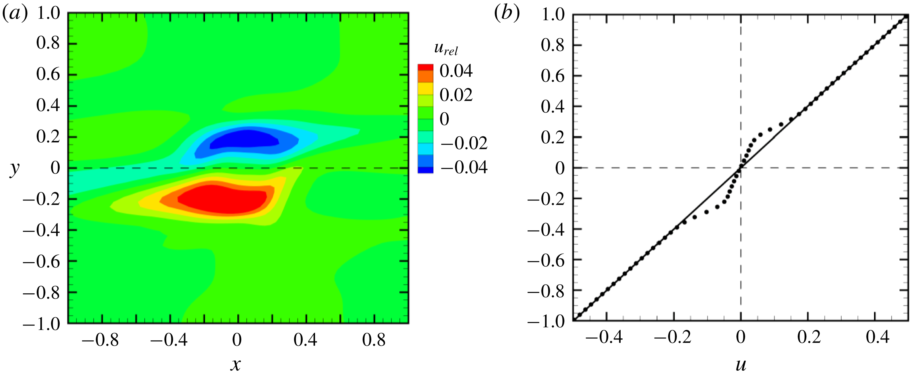
. Consequently, we observe that the particle agglomerate is rotating approximately 30 % more slowly than would a fluid element in the shear flow. This observation is consistent with the findings of Li, Ye & Liu (Reference Li, Ye and Liu2016), who found that a porous circular particle in a two-dimensional shear flow rotates in the flow more slowly than a fluid element. In figure 6(a), we plot contours of the relative fluid velocity in the streamwise (
 $x$
) direction,
 $u_{rel}$
, at time
 $t=20$
, which is typical of the results observed throughout the computation. The relative fluid velocity is found to be oriented in a direction opposite to the ambient shear velocity, with negative value for
 $y>0$
and positive value for
 $y<0$
. A profile of the relative fluid velocity along the
 $y$
-axis (
 $x=z=0$
) is shown in figure 6(b) as dots, with the ambient shear flow drawn as a solid line. We again see that the computed velocity in the region near the agglomerate (
 $|y|<0.4$
) lags behind the ambient shear velocity, which is due to the fact that the particle agglomerate is rotating more slowly than the fluid element so that the forces induced by the particles retard the fluid flow.
(a) Contour plot of the
 $x$
-component
 $u_{rel}$
of the relative velocity in the
 $x$
–
 $y$
plane, for case A.4 at
 $t=26$
. (b) Profile of the
 $x$
-component of velocity
 $u$
along the
 $y$
-axis. The solid line denotes the ambient shear flow and the dots denote the computed velocity profile.

A series of plots in the three cross-sectional planes (
 $x$
–
 $y$
,
 $x$
–
 $z$
and
 $y$
–
 $z$
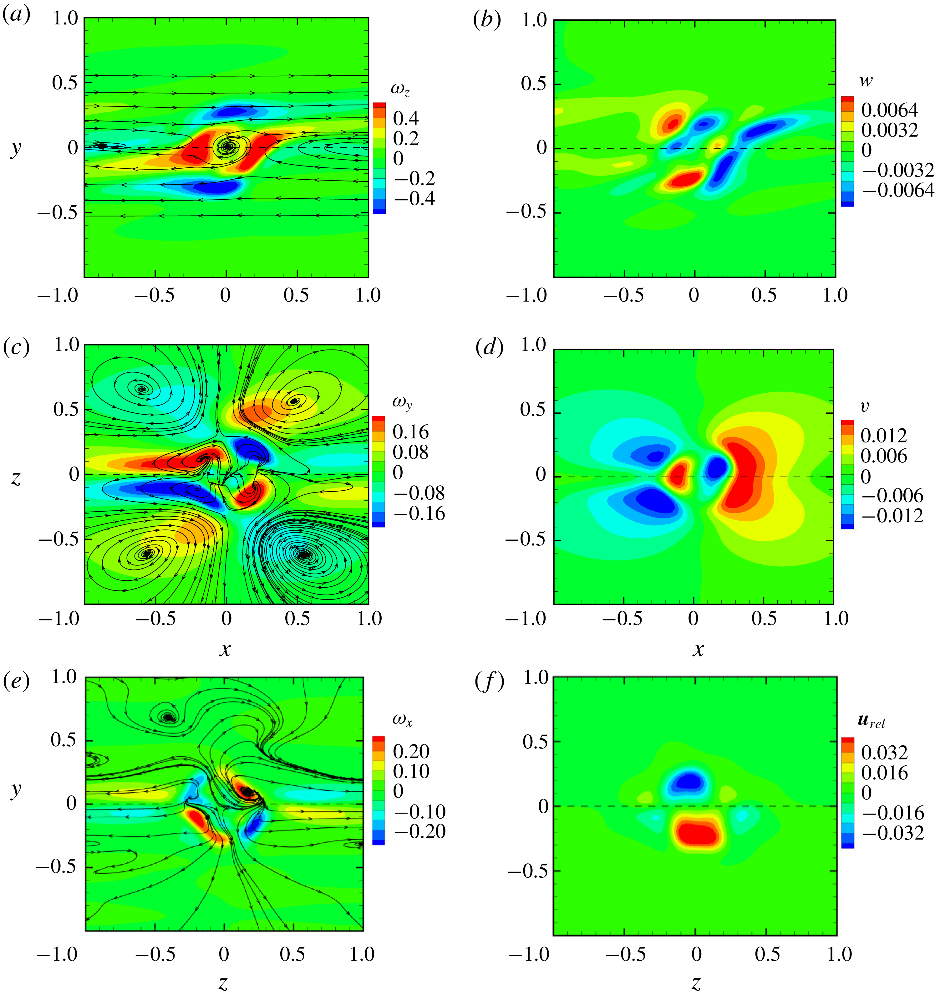
) are shown in figure 7, where for each plane we plot the in-plane streamlines (obtained by setting the normal velocity component to zero) and the contours of both the normal vorticity and velocity components. The plots do not include the entire computational domain, but instead focus on the central part of the domain near the agglomerate. In figure 7(a), the streamlines in the
 $x$
–
 $y$
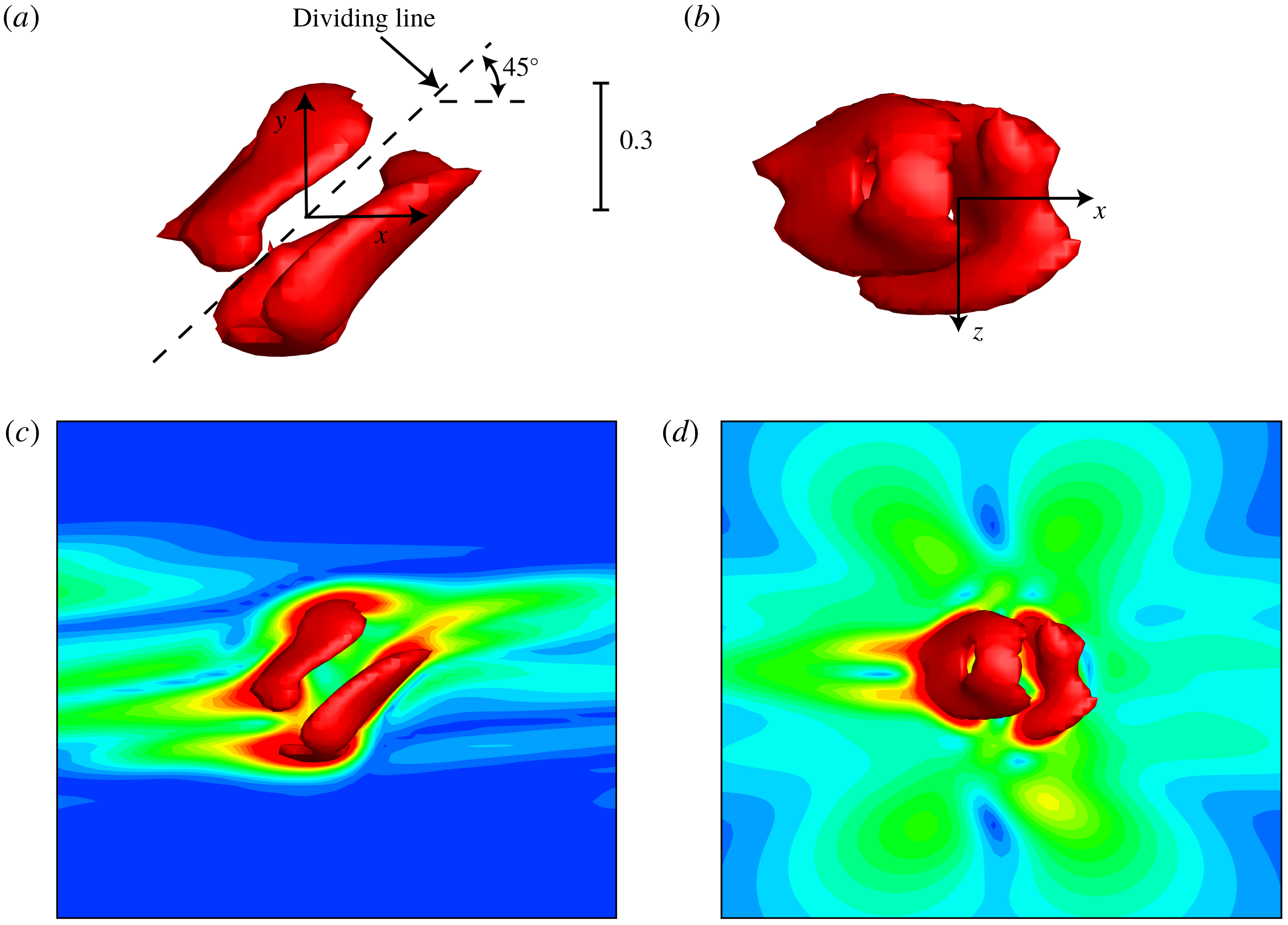
plane are seen to exhibit a vortex at the origin (i.e. at the centre of the agglomerate); however, we note that the fluid velocity near the vortex centre is very weak, and hence the normal vorticity magnitude at the vortex centre is small. In all three cross-sectional planes, the normal vorticity component has a quadrupole structure, with four vorticity patches of alternating sign. From these cross-sectional plots, the velocity and vorticity fields associated with the rotating particle agglomerate appear to have the form of two tilted vortex rings with opposite circulation immersed in the shear flow.
(a,c,e) Contours of normal vorticity and streamlines of the in-plane velocity field and (b,d,f) contours of normal component of the relative velocity
 $\boldsymbol{u}_{rel}$
in three orthogonal planes passing through the agglomerate, for case A.4 at
 $t=26$
.

To better illustrate this flow field, we compute the relative fluid vorticity
 $\unicode[STIX]{x1D74E}_{rel}=\unicode[STIX]{x1D74E}+S\boldsymbol{e}_{z}$
, where we recall that the vorticity of the ambient shear flow is
 $-S\boldsymbol{e}_{z}$
. The isosurface
 $\unicode[STIX]{x1D714}_{rel}=0.46$
of the magnitude of
 $\unicode[STIX]{x1D74E}_{rel}$
is plotted in figure 8 in both the
 $x$
–
 $y$
plane (looking from the side) and the
 $x$
–
 $z$
plane (looking from the top). The same two views of this isosurface are also shown in figure 8 showing contours of
 $\unicode[STIX]{x1D714}_{rel}$
on a slice of the flow field in the normal plane. The
 $\unicode[STIX]{x1D714}_{rel}$
isosurfaces clearly show that the particle-induced flow field for a single rotating agglomerate in a shear flow has the form of a pair of tilted vortex rings of opposite sign, with tilt angle of approximately
 $45^{\circ }$
relative to the ambient shear flow (
 $x$
-direction). As seen in the slices of the flow field in figure 8(c,d), each vortex ring is surrounded by stretched and reoriented vorticity from the ambient shear flow that trails behind the vortex rings in each direction. The dynamics of a single vortex ring in a linear shear flow was studied by Cheng, Lou & Lim (Reference Cheng, Lou and Lim2009), who found that the vortex ring becomes tilted relative to the shear and maintains a ring-like form while it drifts upwards in the shear field (in the
 $y$
-direction). This upward drift is negated in the current situation by the mutually induced flow field when two rings of opposite sign coexist, leading to a quasi-stationary flow with a quadrupole far-field structure (as is evident in the streamlines in figure 7
c). For computations where the shear flow does not trigger breakup of the agglomerate, such as for case A.4, this flow structure is observed to remain nearly constant with time as the agglomerate rotates in the shear flow.
Isosurface of the relative vorticity magnitude
 $\unicode[STIX]{x1D714}_{rel}=0.46$
obtained from the velocity field for case A.4 at
 $t=26$
, showing two tilted vortex rings generated by the particle-induced velocity field near the rotating agglomerate. (a,b) Isosurfaces in the (a)
 $x$
–
 $y$
plane and (b)
 $x$
–
 $z$
plane. (c,d) The same isosurface views together with a slice showing
 $\unicode[STIX]{x1D714}_{rel}$
contours in the normal plane.

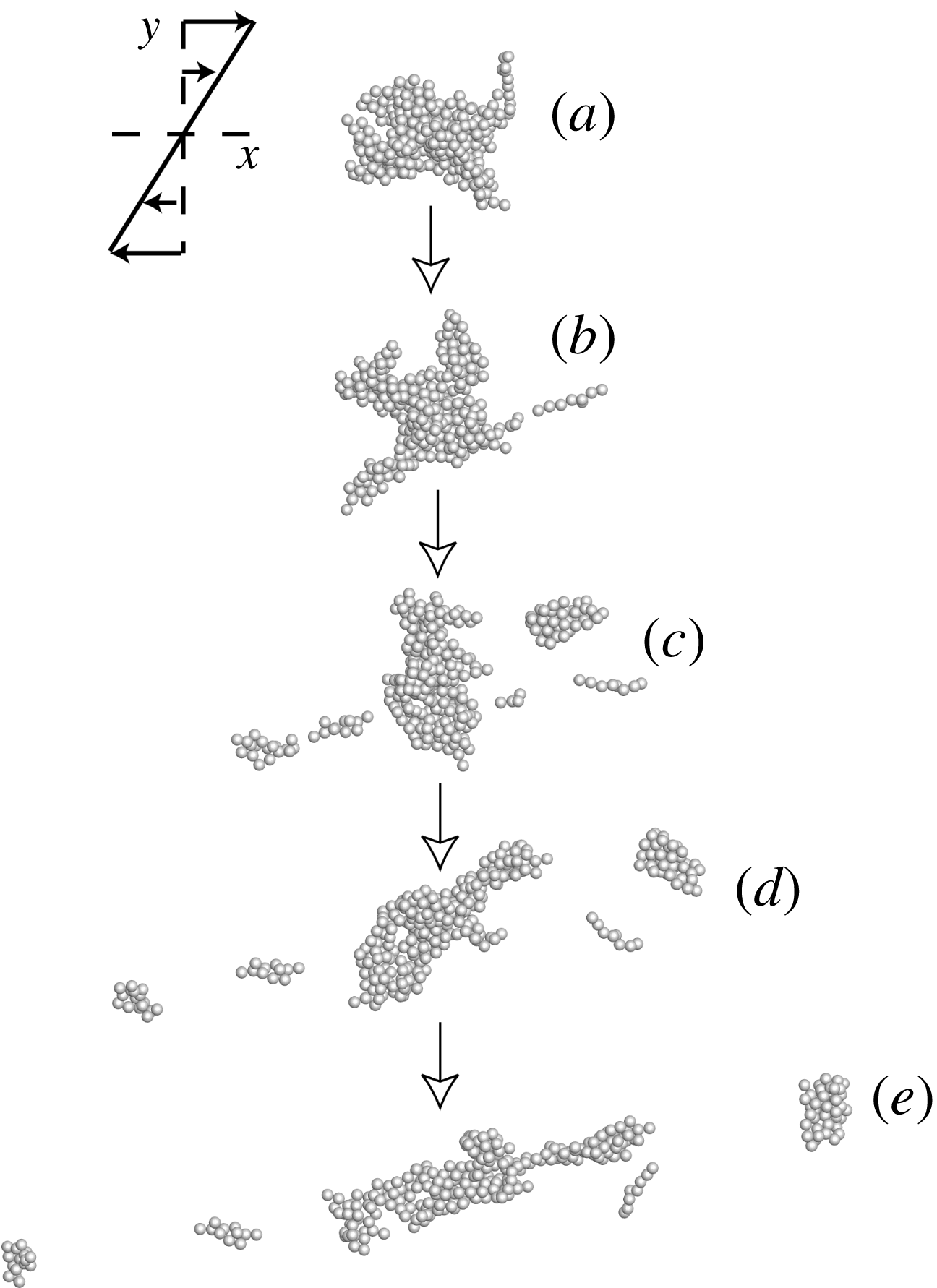
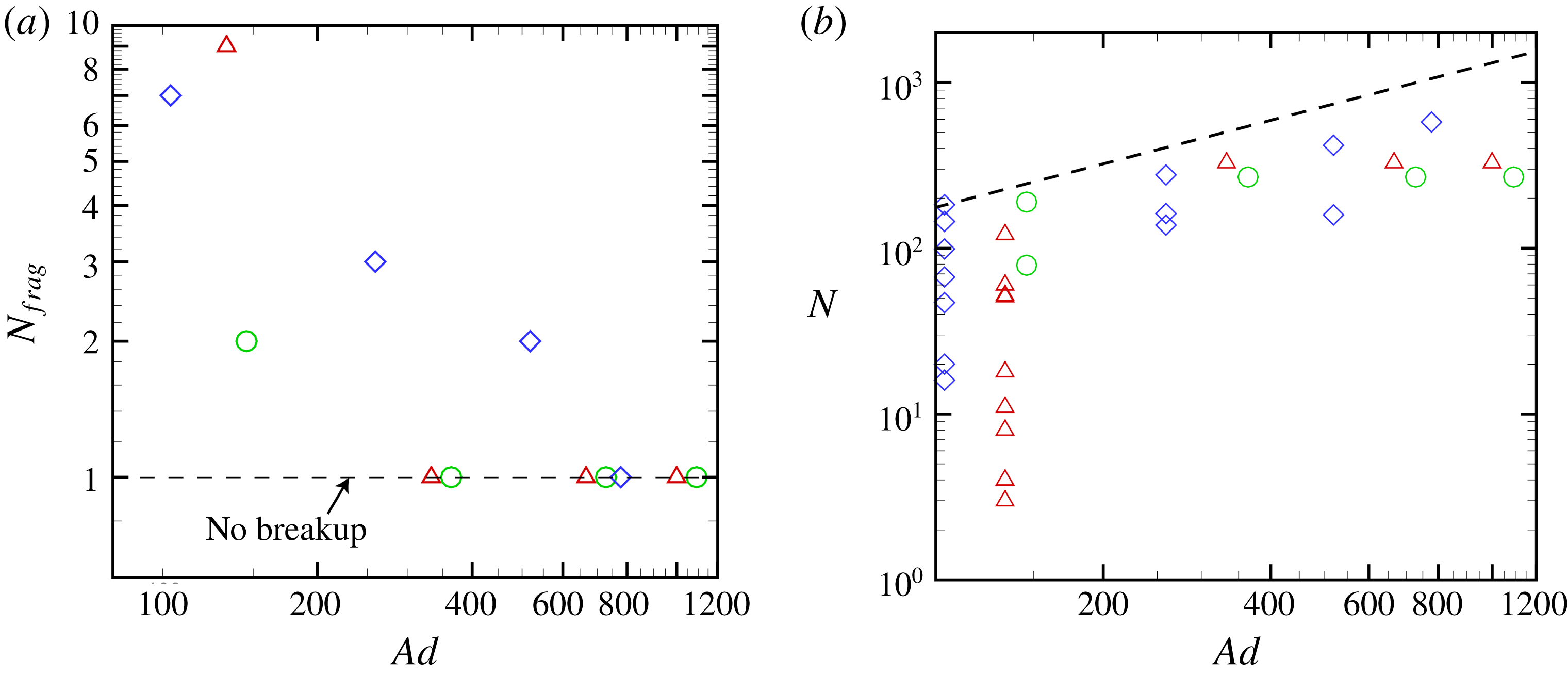
As the adhesion parameter is varied in different computations, different behaviour of the particle agglomerates in the shear flow is observed. For sufficiently low adhesion parameter values, some agglomerates are observed to break up into multiple fragments in the presence of the shear flow. A time series illustrating agglomerate breakup in the shear flow is shown in figure 9 for case A.1. We note from this example that, while the fragments that shed from the agglomerate are limited by the maximum size that the agglomerate can attain without breakup in the shear flow, there are also many agglomerates that are formed of a much smaller size. The set of fragments thus has a wide size distribution. A set of plots summarizing the computed agglomerate evolution for all of the single-agglomerate computations (cases A.1–A.12) is given in figure 10. In figure 10(a), we plot the number of fragments
 $N_{frag}$
into which the agglomerate breaks up as a function of the adhesion parameter
 $Ad$
, defined in (2.22). The data are from three agglomerates extracted from the turbulent agglomeration computation, and different symbols are used in figure 10 to denote the data from each agglomerate. For sufficiently high values of adhesion parameter, the agglomerate does not break up and the value of
 $N_{frag}=1$
in figure 10(a). The number of particles
 $N$
in each fragment at the end of the computation (
 $t=30$
) is plotted versus adhesion parameter in figure 10(b) on a log–log plot. The power-law expression
 $N\propto S^{-0.878}$
of Sonntag & Russel (Reference Sonntag and Russel1986) can be written in terms of the adhesion parameter as
 $N\propto Ad^{0.878}$
. This expression is plotted as a dashed line in figure 10(b), where the coefficient of proportionality is fitted to the data. The expression is found to be a reasonable fit for the maximum values of
 $N$
, thus setting the largest size agglomerates that can survive without breakup in the shear flow.
Time series showing breakup of single agglomerate in a shear flow, for case A.1 at times (a)
 $t=0$
, (b) 5, (c) 10, (d) 15 and (e) 20.

Plots showing measures characterizing breakup of a single agglomerate in a shear flow. (a) Number of fragments into which an agglomerate breaks up versus adhesion parameter. When the agglomerate does not break up,
 $N_{frag}=1$
. (b) Number of particles
 $N$
in agglomerates following breakup versus adhesion parameter. The dashed line is the experimental power-law fit
 $N\propto Ad^{0.879}$
from Sonntag & Russel (Reference Sonntag and Russel1986) for maximum number of particles, where the proportionality coefficient is fitted to the data. The data are plotted for cases A.1–A.4 (red deltas), A.5–A.8 (green circles) and A.9–A.12 (blue diamonds) from table 1.

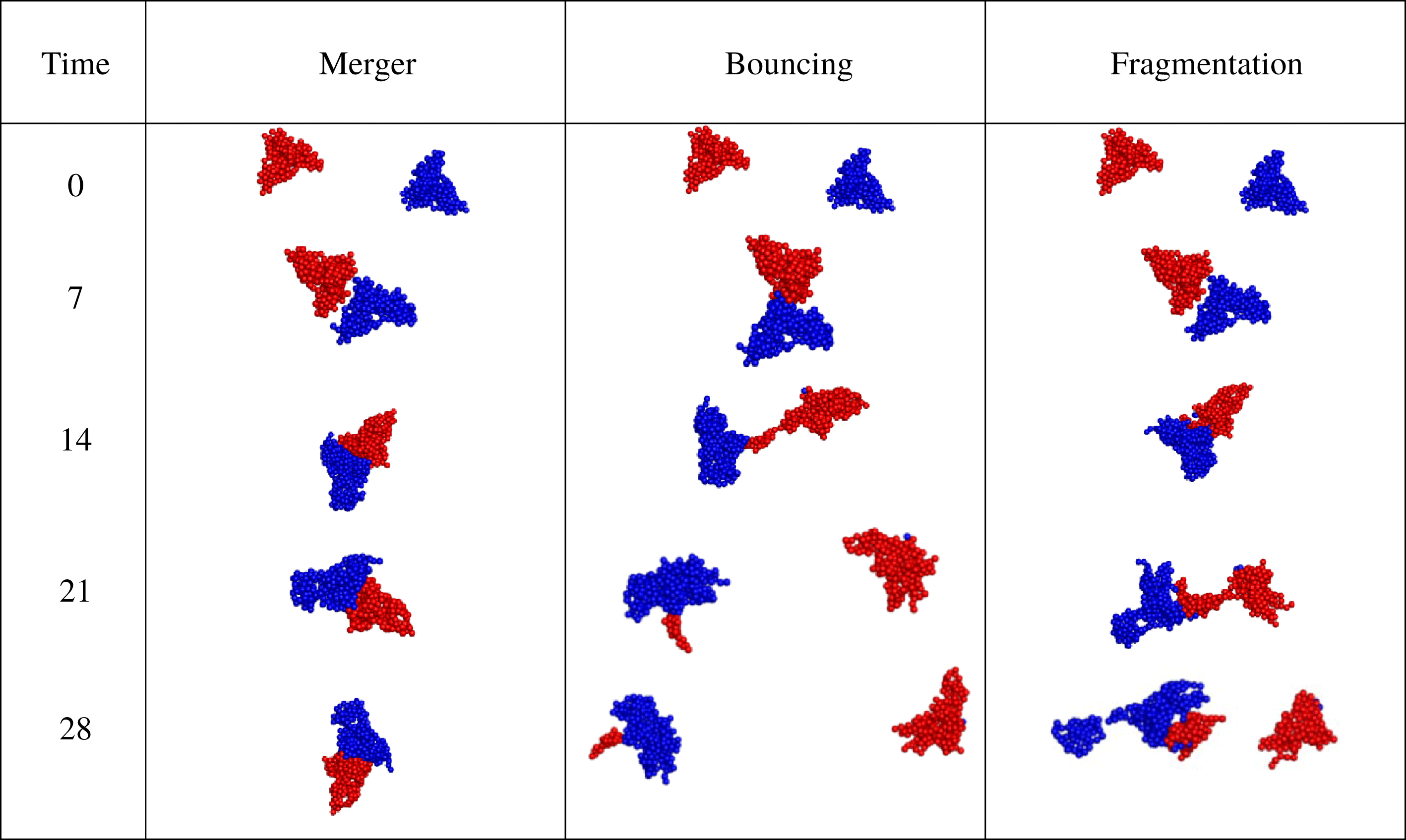
Scatter plots illustrating three types of agglomerate interactions: merger (case B.15), bouncing (case B.19) and fragmentation (case B.13).

4 Agglomerate pair collision in shear flow
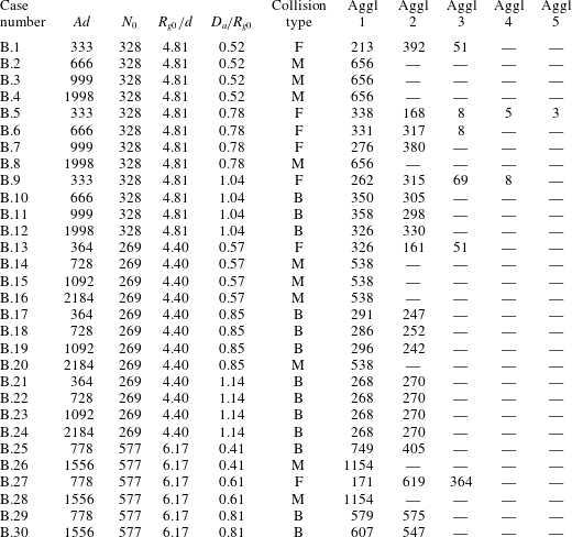
In this section, we examine the collision of two agglomerates in a shear flow. As stated in § 2, each particle in an agglomerate is in contact with at least one other particle in the agglomerate. Two agglomerates collide when at least one particle in each agglomerate come into contact with each other. For the computations of agglomerate collision reported in this section, three different agglomerates were extracted from the turbulent agglomeration computation described in § 2.2, which were used to conduct 30 computations of agglomerate collision, the parameters for which are listed in table 2. For each computation, the agglomerates are initialized as shown in figure 2(b), with orientations of
 $\pm 45^{\circ }$
and displacement of the agglomerate centroid by an amount
 $\pm D_{a}$
in the
 $y$
-direction. Each computation examines collision of an agglomerate with an exact copy, and we did not consider collisions of different size agglomerates. Consideration of the computational results indicates three different types of behaviours, which are illustrated in scatter plots in figure 11. In these plots, each particle is coloured either red or blue to indicate the agglomerate from which the particle originated. The first type of collision outcome is merger of the agglomerates into a single agglomerate, which then rotates in the shear flow. The second type of behaviour, referred to as a bouncing collision, results in two separate agglomerates following the collision. As seen in figure 11, it is common for some particles to be exchanged between the two colliding agglomerates during bouncing collisions. The third type of behaviour is referred to as fragmentation, which describes collisions that result in three or more agglomerates. In the case shown in figure 11, the collision results in three agglomerates – one composed entirely of red particles, one composed entirely of blue particles, and one composed of a combination of red and blue particles. In other cases, more than three agglomerates will form in a fragmentation collision, often yielding a wide variation in agglomerate sizes. Sometimes it is not clear whether a collision should be classified as a bouncing case or a fragmentation case; for instance, cases where two colliding agglomerates break away from each other but leave behind a very small third ‘satellite’ agglomerate composed of just a few particles can be regarded as somewhat in between these two classifications. For purposes of this paper, collisions are classified as bouncing cases if only a single ‘satellite’ particle is separated from the two main agglomerates, and they are classified as fragmentation cases if the satellite agglomerate consists of two or more particles. More typical fragmentation cases are similar to that shown in figure 11, however, producing at least three large agglomerates and sometimes also several smaller agglomerates.
Listing of parameter values for cases examined for collision of two agglomerates, including adhesion parameter (
 $Ad$
), initial numbers of particles in each agglomerate (
 $N_{0}$
), ratio of initial gyration radius (
 $R_{g0}$
) of each agglomerate to particle diameter (
 $d$
), and ratio of initial offset distance (
 $D_{a}$
) to
 $R_{g0}$
. For each case examined,
 $St=1.4$
and
 $\unicode[STIX]{x1D70C}_{p}/\unicode[STIX]{x1D70C}_{f}=10$
. Also listed are the observed type of collision – merger (M), bouncing (B) or fragmentation (F) – and the number of particles in each remaining agglomerate (Aggl 1–5) after the collision.

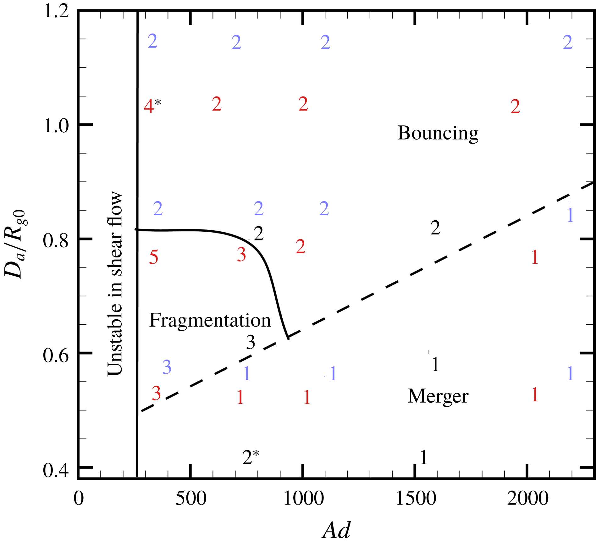
Summary of results for all agglomerate collision runs, showing the number of agglomerates (
 $N_{agg}$
) remaining after collision as a function of adhesion parameter and the ratio
 $D_{a}/R_{g,ave}$
of offset distance to initial radius of gyration. Colours indicate results from different agglomerates. Numbers indicate cases with agglomerate merger (
 $N_{agg}=1$
), bounce (
 $N_{agg}=2$
) and fragmentation (
 $N_{agg}>2$
).

The question of whether a given collision will be of the merger, bouncing or fragmentation type depends primarily on the values of the adhesion parameter
 $Ad$
and the ratio of the
 $y$
-direction offset distance
 $D_{a}$
to the initial radius of gyration
 $R_{g0}$
of the two agglomerates. A plot identifying the type of collision for all computations conducted is shown in a mapping of
 $Ad$
versus
 $D_{a}/R_{g0}$
in figure 12, and details of the number of particles in each agglomerate following collision are listed in table 2. Regions of the map in figure 12 are marked to provide a rough identification of values of
 $Ad$
and
 $D_{a}/R_{g0}$
for which the agglomerates individually break up in the shear flow (to the far left of the plot) and values resulting in merger, bouncing and fragmentation type collisions. The dashed line separating the merger and bouncing regimes is given by the line
 $D_{a}/R_{g0}=0.45+0.0002Ad$
. The numbers indicate the number of agglomerates present at the conclusion of the computation, where an agglomerate is defined as a group of two or more touching particles. In general, collisions resulting in mergers occurred for smaller values of dimensionless offset distance
 $D_{a}/R_{g0}$
and values of
 $Ad$
well above the critical value for breakup of the individual agglomerate in shear flow. Bouncing collisions occur for larger values of
 $D_{a}/R_{g0}$
, resulting in glancing collisions of the agglomerates. Fragmentation occurs for moderate values of
 $D_{a}/R_{g0}$
with adhesion parameter values just slightly larger than the critical value for breakup of a single agglomerate in the shear flow. Two cases in figure 12 requiring special discussion are indicated with asterisks. One of these cases, indicated by
 $2^{\ast }$
, was identified as a bouncing collision because it resulted in two agglomerates, but a much larger number of particles were exchanged between the two agglomerates than was the case for other bouncing collision cases. Indeed, 172 particles originating in the red agglomerate, out of an initial 577 particles, were torn off and captured by the blue agglomerate during the collision. The case indicated by
 $4^{\ast }$
in figure 12 was, on the other hand, a fairly typical fragmentation case, resulting in three fairly large agglomerates with 263, 315 and 69 particles and one smaller ‘satellite’ agglomerate with eight particles. The presence of this fragmentation case in a region where we otherwise see a lot of bouncing cases is a reminder that each agglomerate has its own unique structure and each collision involves different parts of these unique agglomerates, so one must expect substantial variation from case to case. The plot in figure 12 should therefore be regarded as providing only a rough indication of the conditions under which different types of collisions occur and not as a strict regime map.
For the problem of collision of two particles, the criterion for sticking or bouncing of the particles can usually be expressed as a critical value of the particle Stokes number
 $St$
, which is a function of the adhesion parameter
 $Ad$
. Applying this same idea for the problem of agglomerate collision, we can define an agglomerate Stokes number
 $St_{A}$
as the ratio of an agglomerate time scale
 $\unicode[STIX]{x1D70F}_{A}=m_{A}/3\unicode[STIX]{x03C0}\unicode[STIX]{x1D707}R_{g0}$
and the fluid time scale
 $\unicode[STIX]{x1D70F}_{f}=L/U=R_{g0}/SD_{a}$
, giving
 $$\begin{eqnarray}St_{A}=\frac{m_{A}S}{3\unicode[STIX]{x03C0}\unicode[STIX]{x1D707}R_{g0}}\frac{D_{a}}{R_{g0}}.\end{eqnarray}$$
In this expression,
 $m_{A}$
is the agglomerate mass,
 $U=SD_{a}$
is the characteristic velocity difference between the agglomerates, and
 $R_{g0}$
is an agglomerate length scale. The agglomerate Stokes number is therefore found to vary linearly with the ratio
 $D_{a}/R_{g0}$
used in figure 12.
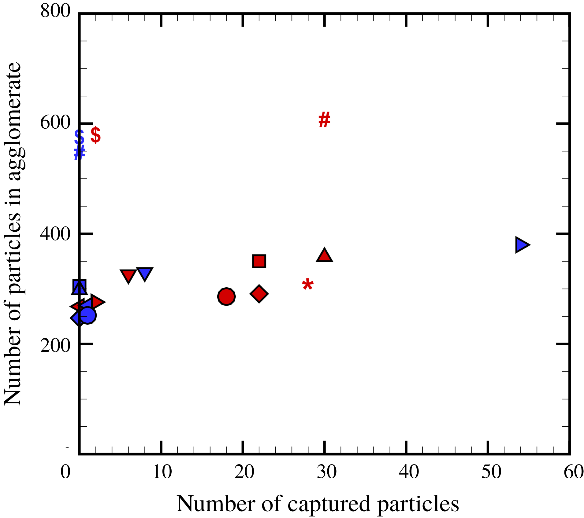
While we have used the term ‘bouncing collision’ to be in conformity with terminology used in previous literature (e.g. Brisset et al. Reference Brisset, Heißelmann, Kothe, Weidling and Blum2016), it is clear that the bouncing agglomerate collisions for the loosely structured agglomerates examined in the current study differ substantially from the traditional bouncing collision of two elastic particles. In a traditional bouncing process, two colliding elastic bodies deform locally near the collision point, resulting in an elastic (or sometimes plastic) repulsion force pushing the two bodies away from each other. In a bouncing case, this repulsion force is sufficiently strong to overcome the adhesive force between the bodies, so that the two bodies will detach and continue to move away from each other. The bouncing collisions of two loosely structured agglomerates observed in the current paper are characterized more by tearing away and eventual capture of particles from the opposing agglomerate by the particle adhesion force. It is not that the elastic force between the agglomerates overcomes the adhesive force between the bodies, but rather that the adhesion force imposed on the captured particles by one agglomerate overcomes the adhesion force from the agglomerate to which the captured particles were originally attached. A plot showing number of captured particles from both agglomerates during the different bouncing collisions computed is given in figure 13. As we see from this plot, all bouncing collisions included captured particles. In some cases only one agglomerate captures particles, and in other cases both colliding agglomerates capture particles from the other agglomerate.
Plot indicating the number of captured particles in bouncing collisions versus the total number of particles in an agglomerate. The number of red particles captured by blue agglomerates is plotted in red, and the number of blue particles captured by red agglomerates is plotted in blue. Different symbols are used to indicate different computations, with one red and one blue symbol for each computation.

While exchange of particles was a characteristic feature of all bouncing collisions, this is not to say that there was no rebound force between the agglomerates. An examination of the rebound force is reported below for the bouncing collision in case B.19, in which 28 particles originating in the red agglomerate are captured by the blue agglomerate and one blue particle is captured by the red agglomerate. The number of touching red–blue particles (i.e. touching particles originating from opposite agglomerates) is plotted as a function of time in figure 14(a). This number is zero until
 $t=5$
, at which time the collision occurs, and then suddenly spikes up to a peak value of 18 at a time of approximately
 $t=6.5$
. After this point the number of touching red–blue particles decreases to 14 and remains there, with the exception of a small blip at
 $t=10$
due to restructuring. The fact that the number of red–blue touching particles does not reduce to zero following the collision is due to the presence of captured particles. The total compressive force between the two agglomerates (which is characteristic of the elastic rebound force) is plotted as a function of time in figure 14(b). We again observe a sudden increase at collision onset at
 $t=5$
and a peak value at
 $t=6.5$
, followed by a gradual decrease of the compression force as the two agglomerates tear away from each other.
Time variation of (a) number of touching particles originating in different agglomerates and (b) total dimensionless compressive force between the agglomerates for a typical bouncing case (case B.19). Collision onset occurs at approximately
 $t=5$
and the agglomerates detach at
 $t=14$
.

The position of particles carrying the compressive load between the two colliding agglomerates is illustrated in figure 15 at a time of
 $t=7$
, close to the peak time of the collision. In figure 15(a), we colour the particle scatter plot with red or blue to identify the originating agglomerate for each particle. In figure 15(b), each particle is coloured by the magnitude of the total compressive force acting on the particle. The highest compressive loads are borne by a core of particles on the inside of the agglomerate, shown in figure 15(c) with the lower-compression particles removed, within a tube of force chains radiating outwards from the collision point. The highest compressive load occurs on the particles just at the collision point, indicated by red or orange in figure 15(c). We have thus confirmed that a rebound force does occur in bouncing collisions, and it may be reasonable to characterize this aspect of the collision phenomenon by some type of effective elastic modulus assigned to an effective spherical body representing the agglomerate. However, this effective sphere representation does not include the important phenomenon of particle capture during bouncing collisions, which in most of the cases that we have examined is very important to the agglomerate behaviour during collision.
Scatter plots during a bouncing agglomerate collision (case B.19) at
 $t=7$
, with colours indicating (a) agglomerate from which each particle originated, (b) total compressive force acting on each particle, and (c) same plot as in (b) with the low-compression particles (with compressive force
 ${<}$
1.5) blanked out. High-compression force chains occur in a particle core region spreading outwards from the collision point.

In § 3, we discussed the observation that the particle-induced flow field from a single agglomerate in a shear flow has the form of two tilted vortex rings of opposite sign. In the event of a collision of two agglomerates, one naturally wonders what happens to the particle-induced flow during the collision. To examine this question, an isosurface of the relative vorticity magnitude
 $\unicode[STIX]{x1D714}_{rel}$
is plotted at four different times during a collision resulting in merger (figure 16 for case B.15) and during a collision resulting in bouncing (figure 17 for case B.19). The relative vorticity isosurface for fragmentation cases depends on the number of fragments produced, and so is highly variable. The agglomerate centroids and initial radius of gyration are indicated in these figures by a black dot and a circle, respectively, for each agglomerate. In the lower part of each panel is given a scatter plot showing the particle positions at that time, with colour used to identify the agglomerate of origin for each particle.
Isosurface of relative vorticity magnitude
 $\unicode[STIX]{x1D714}_{rel}=0.3$
(top) and particle scatter plot coloured by initial agglomerate identity (bottom) for a case where the particle agglomerates merge (case B.15), at times (a)
 $t=6$
, (b) 8, (c) 10 and (d) 12 during which collision and merger of the agglomerates occurs. The agglomerate centroids and initial radius of gyration are indicated in the upper part of each panel by a black dot and a circle, respectively, for each agglomerate.

Isosurface of relative vorticity magnitude
 $\unicode[STIX]{x1D714}_{rel}=0.3$
(top) and particle scatter plot coloured by initial agglomerate identity (bottom) for a case where the particle agglomerates bounce (case B.19), at times (a)
 $t=6$
, (b) 8, (c) 10 and (d) 12 during which collision of the agglomerates occurs. The agglomerate centroids and initial radius of gyration are indicated in the upper part of each panel by a black dot and a circle, respectively, for each agglomerate.

In figure 16, the particle-induced flow field at time
 $t=6$
(just before the collision) has the form of two opposite-sign tilted vortex rings for each agglomerate, hence four tilted vortex rings in all. At time
 $t=8$
the agglomerates are in the midst of colliding and the innermost vortex rings of each agglomerate collide with one another. At
 $t=10$
, the inner vortex rings have significantly decayed while the outer vortex rings have grown in strength. The inner rings continue to break up and be swept downstream by
 $t=12$
, leaving the two strong outer vortex rings, which have opposite sign from each other. With the exception of the small-scale remnants of the inner rings, the particle-induced flow for the merged agglomerates at
 $t=12$
thus appears similar to that for a single agglomerate in a shear flow, as discussed in the previous section, but the vortex rings are larger and stronger for the merged agglomerate.
In figure 17, a time series of relative vorticity magnitude isosurfaces are plotted for a case with bouncing agglomerate collision. The first two images in figure 17 appear similar to those in figure 16 for a merging collision. The two inner rings collide at time
 $t=6$
and nearly extinguish each other by time
 $t=8$
as the agglomerate collision occurs. However, as the agglomerates bounce and move away from each other, the inner rings re-form, such that by
 $t=12$
we see a pair of vortex rings for each agglomerate moving away from each other. A trail of vorticity connects these two vortex ring pairs, which is either left over from the collision or generated by stretching of the background shear vorticity.
5 Conclusions
A computational study was reported examining rotation and breakup of a single particle agglomerate and collision of two particle agglomerates in a shear flow. The agglomerates are extracted from a direct numerical simulation of turbulent agglomeration, and therefore have the characteristic loose fractal structure typical of turbulent agglomeration processes. Computations are performed with four-way coupling between the particles and the fluid and with sufficient resolution of the agglomerates to capture the details of the particle-induced flow field. Simulations of a single agglomerate rotating in the shear flow with high values of the adhesion parameter indicate that the agglomerate rotates more slowly than would an ambient fluid element in the shear flow. The flow field induced by the particles of a rotating agglomerate in a shear flow are found to exhibit a very distinctive form, characterized by a pair of tilted vortex rings with opposite-sign circulation, surrounded by a sea of stretched vorticity from the ambient shear flow. To our knowledge, this is the first time that the particle-induced flow of an agglomerate in shear flow has been examined in detail and the first time that the interesting vortex ring pair structure of this flow has been described. This vortex ring pair structure remains with constant orientation and strength as the particle agglomerate rotates. For sufficiently low values of the adhesion parameter, the agglomerate is observed to break up in the shear flow, where the exact value of the adhesion parameter at breakup varies slightly with the specific choice of the agglomerate under examination.
The problem of collision of two agglomerates was found to result in either merger, bouncing or fragmentation, depending on the value of the adhesion parameter and the ratio of offset distance to agglomerate radius of gyration. In merger collisions, the inner vortex rings of the particle-induced flow from each agglomerate interact with each other and eventually break up into small-scale structures, and the outer vortex rings grow stronger, leading to development of the vortex ring pair structure typical of that observed for a single agglomerate. It was observed that bouncing collisions result in both repulsive force between the agglomerates due to elastic deformation as well as exchange of particles between agglomerates. The innermost vortex ring structures of the particle-induced flow for bouncing collisions similarly exhibit interaction of the two inner vortex rings, but these inner rings are found to quickly re-form as the agglomerates bounce and move away from each other. Fragmentation collisions may result in three or more agglomerates with widely different sizes, many of which are formed of a combination of particles originating in different agglomerate structures.
Many theoretical and computation models of turbulent agglomeration processes make use of the common approximation that an agglomerate can be replaced by an ‘effective particle’, in which some effective elastic modulus of the agglomerate is assigned. The current study demonstrates that this effective particle approximation omits certain important physical phenomena associated with agglomerate collision, including fragmentation collisions (resulting in three or more agglomerates) and exchange of particles between agglomerates in bouncing collisions. The particle-induced flow field is also quite different for a loosely structured agglomerate than it is for an equivalent sphere due to the fact that the fluid flow can penetrate into the outer parts of the agglomerate. This penetration affects the rotation rate of an agglomerate in a shear flow and gives rise to the tilted vortex ring structure of the particle-induced flow.
The current study suggests the need for future work in a number of areas. The current study has focused on collision of particle agglomerates with exact copies of themselves, using a relatively small number of agglomerates in order to focus on the effect of the adhesion number and the spacing ratio
 $D_{a}/R_{g0}$
. There is a need to conduct runs with a larger number of agglomerates, including cases involving collisions of agglomerates of different sizes. The current study considered agglomerates suspended in a simple shear flow, whereas in practice agglomerates will also experience a mean drift relative to the surrounding flow, either from inertia or from a body force such as gravity. An agglomerate falling under gravity in a fluid is known to induce a single vortex ring within the agglomerate (Nitsche & Batchelor Reference Nitsche and Batchelor1997), in contrast to the pair of tilted vortex rings that we have observed to be induced by an agglomerate in a shear flow. The particle-induced flow for an agglomerate experiencing a combination of shear and mean drift would therefore be of interest for future study. Finally, resolution of the flow within the agglomerate using the CFD-DEM approach employed in the current paper requires that the agglomerate size is significantly larger than the particle size. It would be of interest to examine fluid flow effects and collision of smaller agglomerates, for which a computational method capable of resolving flow around individual particles would be necessary.
Acknowledgement
This research was supported by the US National Science Foundation under grants CBET-1332472 and DGE-1144388.