NOMENCLATURE
- (–)
- U
-
conservative vector
- F
-
convective fluxes
- G
-
viscous fluxes
- L
-
objective functions
- D
-
design variables
-
 $\mathbf{X}_{SG}$
-
surface mesh positions
-
$\mathbf{X}_{TG}$
-
interior mesh positions
-
$\Lambda$
-
stiffness matrix of mesh motion equations
-
$C_{j}$
-
force coefficients
-
$a_{j}$
-
weight coefficient
- X
-
local coordinate vector
- B
-
Bernstein polynomial
-
$\mathbf{G}_{s}$
-
surface mesh position on FFD box
-
$C_{l}$
-
lift coefficient
-
$C_{d}$
-
drag coefficient
-
$C_{d}^{P}$
-
pressure drag coefficient
-
$C_{d}^{f}$
-
friction drag coefficient
-
$C_{m}^{y}$
-
pitching moment coefficient
- K
-
lift-to-drag ratio


Greek symbols
- (deg)
-
$\alpha $
-
angle-of-attack

0.1 Acronyms
- UAV
-
unmanned aerial vehicle
- AoA
-
angel-of-attack
1.0 INTRODUCTION
Rapid deployment of one or more surveillance unmanned aerial vehicle (UAV) has gained lots of attention from both military and civilian perspectives. The portability is the most important feature of this type of aircraft. The limited payload requires a careful design for the aerodynamic configuration, structures, control system and so on, all of these lead to a very wide spectrum of considerations. The main duties of UAVs are reconnaissance and discovery for a specific field, for instance to give a reliable answer to soldier of what’s over the next hill. From this point, the size should not be as large as the common UAV, such as RQ from the United States or CH from China. The small UAV — or the even smaller alternatives such as micro air vehicles (MAVs) — is appropriate for the close-range and low-attitude detecting and sensing missions, which makes this airplane a man-portable device. Gabriel et al.(Reference Gabriel and Mueller1) proposed that the technical indicators for a MAV are as follows: maximum dimension of 15cm, operating range of 10km, average endurance of 30min, payload capability up to 18g, and autonomous or semi-autonomous control. The payload, obviously, is the important parameter needed to be enhanced for a better performance.
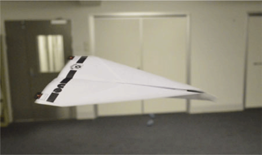
The low-cost feature is always a basic requirement of a man-portable weapon or device; however, the typical driven equipment inside a MAV is very complicated. Some researchers, such as Schluter(Reference Schlüter2), presented a detailed experimental study of a paper plane, which, evidently, has a very performance for the cost control. Pounds et al.(Reference Pounds and Singh3) performed a feasible solution based on disposable paper UAV (Fig. 1) including inertial sensors and elevons, which endow the UAV’s more complicated functions and makes it programmable. The commonly used aerodynamic configuration for a paper plane is delta-wing type, which always has a small aspect ratio, that is, the lift mechanisms can be summarised in terms of two aspects: a linear part induced by the existence of circulation around the foil, and a nonlinear part induced by the strong wingtip vortices. The linear part can be modeled with theory and relate to the profile. Correspondingly, the nonlinear part which providing vortex lift is affected by the wing platform, aspect ratio and rake Angle of the leading edge. For example, Gabriel(Reference Gabriel and Mueller1) found that the low-aspect ratio to have high values of maximum lift coefficient. Kaplan et al.(Reference Kaplan, Altman and Ol4) studied the wake for delta-wing configuration at three Reynolds numbers and found that a constant aspect ratio with different wing platform and Reynolds number barely changed the slope of the lift curve. The leading-edge vortices, which are responsible for the nonlinear lift, have great relation with the type of leading edge and swept angles. In addition, the Reynolds number, demonstrated by Luckring(Reference Luckring5), has dramatic influence on the separation-induced leading-edge vortex flows, but this factor can be neglected by the paper plane for its operating condition.
Disposable paper UAV.(Reference Pounds and Singh3)

As far as the aerodynamic optimisation problems are concerned, Boschetti et al.(Reference Boschetti, Cárdenas and Amerio6) provide a classical workflow to enhance the lift-to-drag ratio with both experimental and numerical approaches. Secanell et al.(Reference Secanell, Suleman and Gamboa7, Reference Secanell, Suleman and Gamboa8) presented a two-dimensional optimisation of airfoil of the UAV with gradient-based methods, and an obvious enhancement on performance of UAV is obtained. Many works based on global search schemes(Reference Rajagopal and Ganguli9–Reference Kontogiannis and Ekaterinaris13) have proved to be efficient; however, it is hard to extend the design interest to a three-dimensional design process because that large amount of design variables is not acceptable. Correspondingly, many gradient-based methods focus on the use of adjoint variable formulas to obtain sensitivity information(Reference Jameson, Martinelli and Pierce14). The capability of handling with the large number of design variables with few constraints attracted lots of concerns. Examples of both continuous and discrete approaches to this method can be found in Refs. Reference Nadarajah and Jameson15–Reference Bueno-Orovio, Castro, Palacios and Zuazua22.
The work presented in this paper is later used as a basis for developing the aerodynamic configuration of a similar paper plane UAV presented by Pounds et al.(Reference Pounds and Singh3). The aerodynamic optimisation of this paper plane will focus on the airfoil, planform and winglet of the airplane. We also apply the discrete adjoint method included in an unstructured-mesh-based flow solver in the present work.
2.0 NUMERICAL METHODOLOGY
2.1 Governing equations
The compressible Navier-Stokes equations are considered here. The equations are written in conservative form, viz.
 \begin{equation}\begin{array}{*{20}{c}}{\frac{{\partial {\rm{U}}}}{{\partial t}} + \nabla \cdot \left( {{\bf{F}}\left( {\bf{U}} \right) + {\bf{G}}\left( {\bf{U}} \right)} \right)=0}\end{array}\end{equation}
where U indicates the vector of conservative variables which contains mass, momentum, and energy. F(U) and G(U) denote the convective fluxes and viscous fluxes, respectively.
An in-house solver Xenium, which works on unstructured mesh, is used in present paper. The governing equations shown above are discretised via a finite volume method, and the conservative flow variables are expressed with cell-centered evaluation. F(U) is discretised using a flux difference formula developed by Roe(Reference Roe23) and using the MUSCL approach(Reference Colella31) with Venkatakrishnan limiter(Reference Venkatakrishnan24), however, no limiter is used in the present paper. A centered formula is used for the diffusive flux G(U). The gradients of velocity and temperature are evaluated at the center of each cell interface. For turbulent flow, the Boussinesq assumption is used for a Reynolds stress tensor. The eddy viscosity is calculated with the Spalart-Allmaras model(Reference Spalart and Allmaras25), which is solved loosely coupled to the mean-flow equations. A backward Euler time-differencing scheme is used to update the solution, and the linear system of equations is approximately solved with a multicolour point-implicit procedure or an implicit-line relaxation scheme at each time step(Reference Darmofal26, Reference Saad and Schultz27).
2.2 Adjoint equations
The objective function is defined as:
 \begin{equation}\begin{array}{*{20}{c}}{L\left( {\bf{D}} \right) = L\left( {{F_1}\left( {\bf{D}} \right)\!,{F_2}\left( {{F_1}} \right)\!,{F_3}\left( {{F_2}} \right)} \right)\;}\end{array}\end{equation}
where D is design variables. The functions F 1, F 2 and F 3 have the following forms:
 \begin{equation}\begin{array}{*{20}{c}}{{{\bf{X}}_{SG}} = {F_1}\left( {\bf{D}} \right)\!;\;\;\;\;\;{{\bf{X}}_{TG}} = {F_2}\left( {{F_1}} \right)\!;\;\;\;\;\;Q = {F_3}\left( {{F_2}} \right)\!;\;\;\;\;\;L = L\left( {{\bf{Q}},{{\bf{X}}_{TG}}} \right)}\end{array}\end{equation}
The variation of surface mesh after changing the design variables is denoted as X SG. Moreover, the new mesh from X SGcould be generated with function F 2. The predicted variables of flow field based on the new mesh is represented by Q. The sensitivity derivatives can be obtained after a straightforward differentiation of Equation (2):
 \begin{equation}\begin{array}{*{20}{c}}{\frac{{dL}}{{d{\bf{D}}}} = \frac{{\partial L}}{{\partial {\bf{Q}}}} \cdot \frac{{\partial {\bf{Q}}}}{{\partial {{\bf{X}}_{TG}}}} \cdot \frac{{\partial {{\bf{X}}_{TG}}}}{{\partial {{\bf{X}}_{SG}}}} \cdot \frac{{\partial {{\bf{X}}_{SG}}}}{{\partial {\bf{D}}}} + \frac{{\partial {\rm{L}}}}{{\partial {{\bf{X}}_{{\rm{TG}}}}}} \cdot \frac{{\partial {{\bf{X}}_{TG}}}}{{\partial {{\bf{X}}_{SG}}}} \cdot \frac{{\partial {{\bf{X}}_{{\rm{SG}}}}}}{{\partial {\bf{D}}}}}\end{array}\end{equation}
Two sensitivities in Equation (4) are ready to be obtained; that is, the gradient of surface mesh to the design variables,
 $\;\partial {{\bf{X}}_{SG}}/\partial {\bf{D}}$
, and the gradient of interior mesh to the surface mesh,
 $\;\partial {{\bf{X}}_{TG}}/\partial {{\bf{X}}_{SG}}$
, means that a tiny surface movement could lead to a corresponding motion of interior mesh, and this process is written as:
 \begin{equation}\begin{array}{*{20}{c}}{\left[ {\rm{\Lambda }} \right]\delta {{\bf{X}}_{TG}} = \delta {{\bf{X}}_{SG}}\mathop \Rightarrow \limits^{\rm{\;}} {{\left[ {\rm{\Lambda }} \right]}^{ - 1}} = \frac{{\partial {{\bf{X}}_{TG}}}}{{\partial {{\bf{X}}_{SG}}}}}\end{array}\end{equation}
where
 $\left[ {\rm{\Lambda }} \right]$
stands for the stiffness matrix of the mesh motion equation.
A converged state for Navier-Stokes equations has a zero residual, i.e.,
 ${\bf{R}}\left( {{\bf{Q}},{{\bf{X}}_{TG}}} \right)=0$
, could be used to obtain the term ∂
 ${\bf{Q}}$
/∂X
TGwithin a linearised relation:
 \begin{equation}\begin{array}{c}{\left[ {\frac{{\partial {\bf{R}}}}{{\partial {\bf{Q}}}}} \right]\frac{{\partial {\bf{Q}}}}{{\partial {{\bf{X}}_{TG}}}} = - \frac{{\partial {\bf{R}}}}{{\partial {{\bf{X}}_{TG}}}}\mathop \Rightarrow \frac{{\partial {\bf{Q}}}}{{\partial {{\bf{X}}_{TG}}}} = - {{\left[ {\frac{{\partial {\bf{R}}}}{{\partial {\bf{Q}}}}} \right]}^{ - 1}}\frac{{\partial {\bf{R}}}}{{\partial {{\bf{X}}_{TG}}}}}\end{array}\end{equation}
Hence, Equation (4) could be written as follows with considering the above expressions:
 \begin{equation}\begin{array}{*{20}{c}}{\frac{{dL}}{{d{\bf{D}}}} = - \frac{{\partial L}}{{\partial {\bf{Q}}}} \cdot {{\left[ {\frac{{\partial {\bf{R}}}}{{\partial {\bf{Q}}}}} \right]}^{ - 1}}\frac{{\partial {\bf{R}}}}{{\partial {{\bf{X}}_{TG}}}}{{\left[ {\rm{\Lambda }} \right]}^{ - 1}}\frac{{\partial {{\bf{X}}_{SG}}}}{{\partial {\bf{D}}}} + \frac{{\partial L}}{{\partial {{\bf{X}}_{TG}}}}{{\left[ {\rm{\Lambda }} \right]}^{ - 1}}\frac{{\partial {{\bf{X}}_{SG}}}}{{\partial {\bf{D}}}}}\end{array}\end{equation}
After transposing the above equation, the adjoint model can be obtained as:
 \begin{equation}\begin{array}{*{20}{c}}{\frac{{d{L^T}}}{{d{\bf{D}}}} = \frac{{\partial {{\bf{X}}_{SG}}^T}}{{\partial {\bf{D}}}}{{\left[ {\rm{\Lambda }} \right]}^{ - T}}\left[ {\frac{{\partial {L^T}}}{{\partial {{\bf{X}}_{TG}}}} - \frac{{\partial {{\bf{R}}^T}}}{{\partial {{\bf{X}}_{TG}}}}{{\left[ {\frac{{\partial {\bf{R}}}}{{\partial {\bf{Q}}}}} \right]}^{ - T}}\frac{{\partial {L^T}}}{{\partial {\bf{Q}}}}} \right]}\end{array}\end{equation}
A sequential process is needed to solve the adjoint functions shown above. Details could be found in Ref. (Reference Darmofal26, Reference Jameson and Kim28).
2.3 Cost functions
The current work only includes steady-state optimisation, but there still exists multi-objective problems. An explicit relation between cost function and constraints is built as:
 \begin{equation}\begin{array}{*{20}{c}}{{L_i} = \mathop \sum \limits_{j=1}^{{J_i}} {a_j}{{\left( {{C_j} - C_j^{\ast}} \right)}^{{P_j}}}}\end{array}\end{equation}
Here, L iis the cost function, C jis an aerodynamic coefficient, e.g., lift or drag coefficients, the superscript * indicates the user-defined target for the specific coefficient C j, and p jis a manual exponent to control the curvature of L i. The index i implies different cost functions or constraints, which are very useful for multi-objective design or desired sensitivities. For unsteady simulation, the above equation only needs to be multiplied by a time scale. The optimised model used in present study is:
 \begin{equation*}Maximise\;\;K\left( {\bf{D}} \right)\end{equation*}
 \begin{equation}\begin{array}{*{20}{c}}{Subject\;\;to\;:\left\{ {\begin{array}{c}{\frac{{\left| {C_m^y - C_m^{{y^{\ast}}}} \right|}}{{\left| {C_m^{{y^{\ast}}}} \right|}} \le 0.3}\\ \qquad\quad\ {{C_d} \le C_d^{\ast}}\end{array}} \right.}\end{array}\end{equation}
Hence, the objective function is given as:
 \begin{equation}\begin{array}{*{20}{c}}{L=10\left( {{C_d} - C_d^{\ast}} \right)}\end{array}\end{equation}
2.4 Shape and mesh deformation
The free-form deformation (FFD) developed by Samareh(Reference Samareh29) was used herein, and the geometry is parameterised by the coordinates of the lattice box points, which allow a broad range of deformations with a low number of parameters and a smooth deformation. Namely, the surface mesh of an airfoil or wing (or other geometry) is parameterized as a Bézier solid.
The lattice box can be expressed by the following formulation:
 \begin{equation}\begin{array}{*{20}{c}}{X\left( {s,t,u} \right) = {X_0} + \mathop \sum \limits_{i,j,k=1}^{l,m,n} {P_{i,j,k}}B_i^l\left( s \right)B_j^m\left( t \right)B_k^n\left( u \right)}\end{array}\end{equation}
where s, t, u
 $\in$
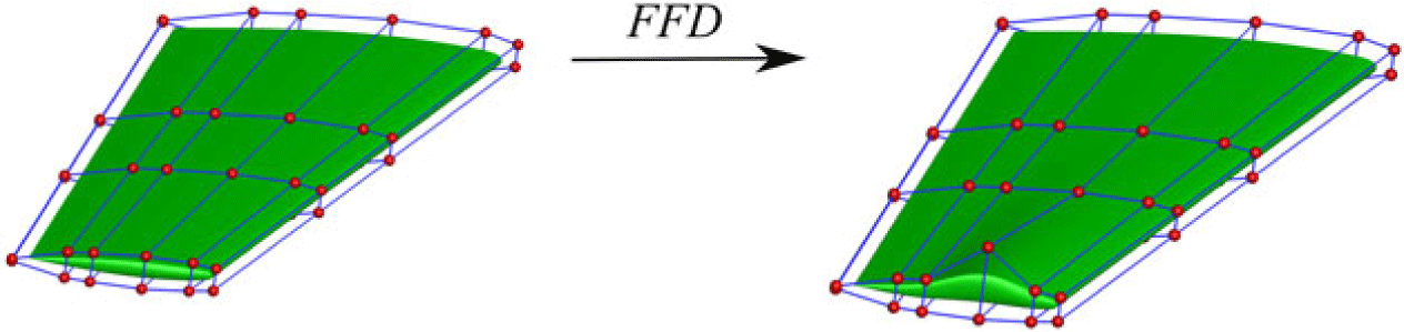
[0, 1] are the three components of the local coordinate, respectively. The X 0 stands for the original point of the local coordinate. B iis the Bernstein polynomial of order i. Then the relation between Cartesian coordinates on the surface mesh and the FFD box was built. The shape of the surface mesh can be changed through varying the control points (design variables) of the box. An example of FFD control point deformation to a wing geometry is demonstrated in Fig. 2.
An example of the FFD technique applied to the 3D wing deformation.

3.0 RESULTS AND DISCUSSIONS
3.1 The performance of the baseline model
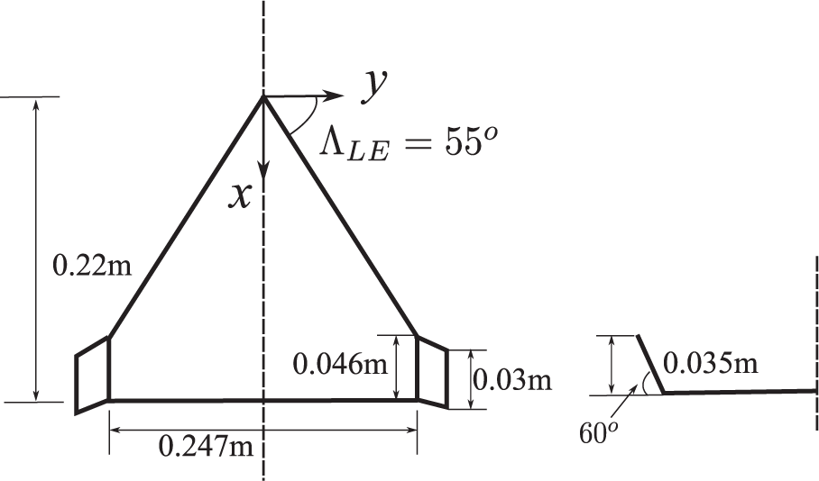
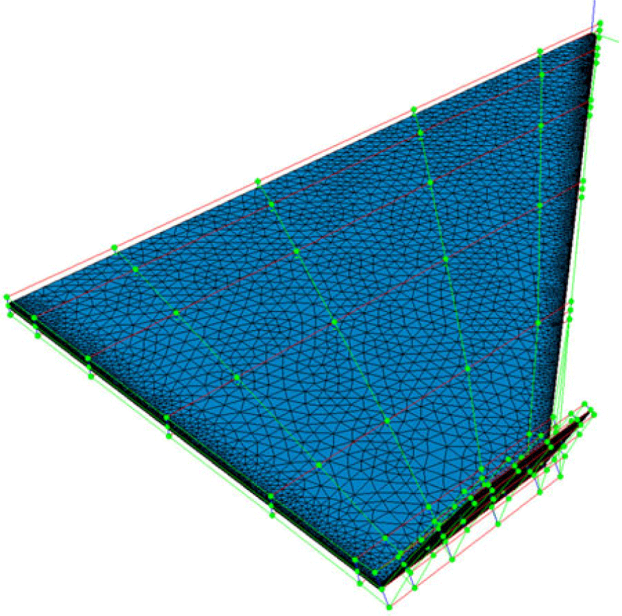
The geometric information of UAV studied by present work is demonstrated in Fig. 3. The freestream velocity U ∞ = 10m/s was adopted to achieve a Reynolds number Re = 80,000 based on a chord length c = 0.154m. The spanwise length and area of the airplane are 0.287m and 0.017m2, respectively. Up to 128 points are used to control the box around the UAV, plotted in Fig. 4, which will give enough space for the geometrical variation.
The detailed geometric size of model used in present work.

The control box and point around the surface mesh.

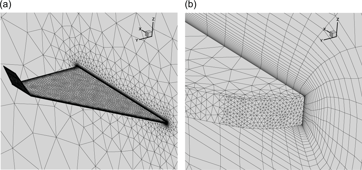
The mesh includes 0.25 million tetrahedral cells and 2 million prism cells (Fig. 5(a)). The near-wall region is refined to provide reasonable velocity gradient of shear layer and boundary layer with a Δy+ of less than 1(Fig. 5(b)). The evolution of the induced vortices is important for the delta-wing-like configuration, hence the volumetric refinements were used at the lee side of the airplane.
Details of the grid for the paper plane. (a) Surface mesh. (b) The refinements for the near-wall region.

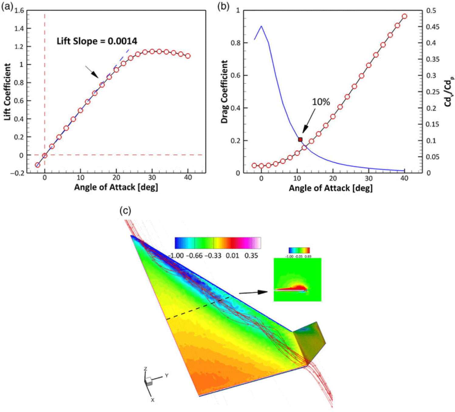
The performance of baseline configuration of the paper plane is demonstrated in Fig. 3.1. The lift slope is roughly 0.0014 with a stall angle of 30deg. As shown in Fig. 6(a), the lift coefficient C l=0 implies the profile of the paper plane does not provide any lift due to its symmetrical geometry. The lift coefficient does not descend very quickly, which can be regarded as a common feature of delta wing(Reference Gursul30), due to the vortex-induced lift. The drag curve is plotted in Fig. 6(b), an obvious increase is after
 $\alpha $
> 13deg. The reason is that the ratio of pressure drag
 $C_d^p$
to viscous drag
 $C_d^v$
becomes larger than the value of 10% as shown by the blue line in Fig. 6(b), which means the pressure drag is the main target to optimise.
Aerodynamic performance of the baseline paper plane. (a) Lift curve. (b) Drag curve. (c) Flow stream traces.

Fig. 6(c) shows the flow chart that the stream traces and surface pressure distribution at the near-wall region. The leading vortices induced a low-pressure region at the first half of the streamwise length of the paper plane.
3.2 Effect of profile inside the delta wing
The optimisation of the present study was based a multi-objective task. Because of the uncertainty of the near-ground atmosphere, which may lead a rapid and large variation of angle-of-attack, a small angle-of-attack
 $\alpha =4$
deg and a high one
 $\alpha=14 $
deg were selected to be the two flow conditions. In this process, the dual optimisations are combined with the basis of better performance has been obtained at two different flow conditions. The objective of present work will be given as:
 \begin{equation}\begin{array}{*{20}{c}}{{L_i} = \mathop \sum \limits_{j=1}^2 \left[ { - {K_j} + \left( {{C_d} - C_d^{\ast}} \right)} \right]}\end{array}\end{equation}
where K is the lift-to-drag ratio. The objective function consist a penalty factor is that the drag coefficient could not increase. Accordingly, if the drag increases compared to the original one, the objective value, that is, the lift-to-drag ratio, would be penalised to a lower value.
The streamwise profiles of the paper plane is the first case to be optimised. The initial profile is a rectangle, which is the slice of a flat plate. The decrement of the force coefficients is evaluated with the function:
 \begin{equation}\begin{array}{*{20}{c}}{\Delta {C_i} = \frac{{\left( {C_i^{opt} - C_i^{base}} \right)}}{{C_i^{base}}} \times 100}\end{array}\end{equation}
where the superscripts opt and base stands for the optimised and baseline configuration. Moreover, the index i denotes lift or drag coefficient.
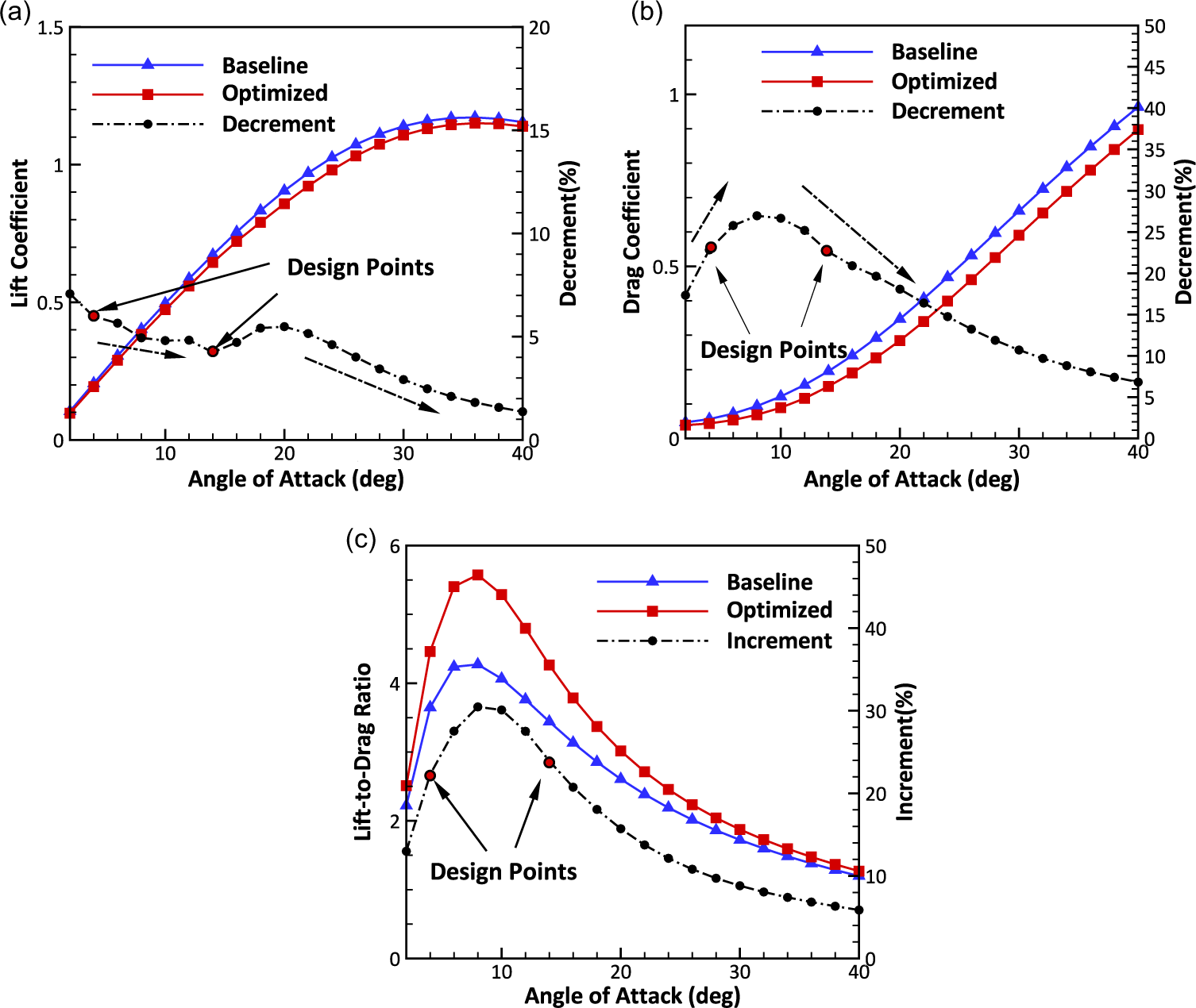
As shown in Fig. 7(a), the lift coefficient of optimised configuration has a less than 7% decrease, and the first design point (α = 4deg) and second design point (α = 14deg) have 6% and 4% lift loss, respectively. However, the difference is shrinking as the increasing α after α = 20deg. The drag coefficient, which is plotted in Fig. 7(b), shows a maximum 27% drag reduction at α = 10deg. As the increasing denominator in Equation (14) and the equivalent distance in Fig. 7(b), a constant drop of
 $\Delta$
C d is readily understood. The decrement of drag of optimised geometry is an order of magnitude larger than that of baseline. The lift-to-drag ratio, K, which is demonstrated in Fig. 7(c), can be easily obtained. The maximum value has a 30% enhancement at α = 8deg, which locates between the dual design points. Although the improvement damped as the increasing angle-of-attack, more than 5% kept even in the large angle.
Optimisation for the profiles. (a) Lift curve (b) Drag curve (c) Lift-to-drag ratio.

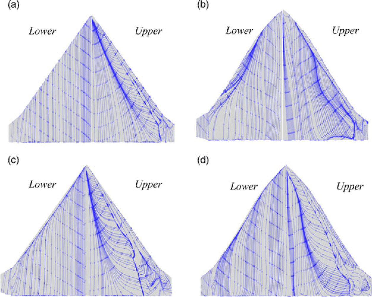
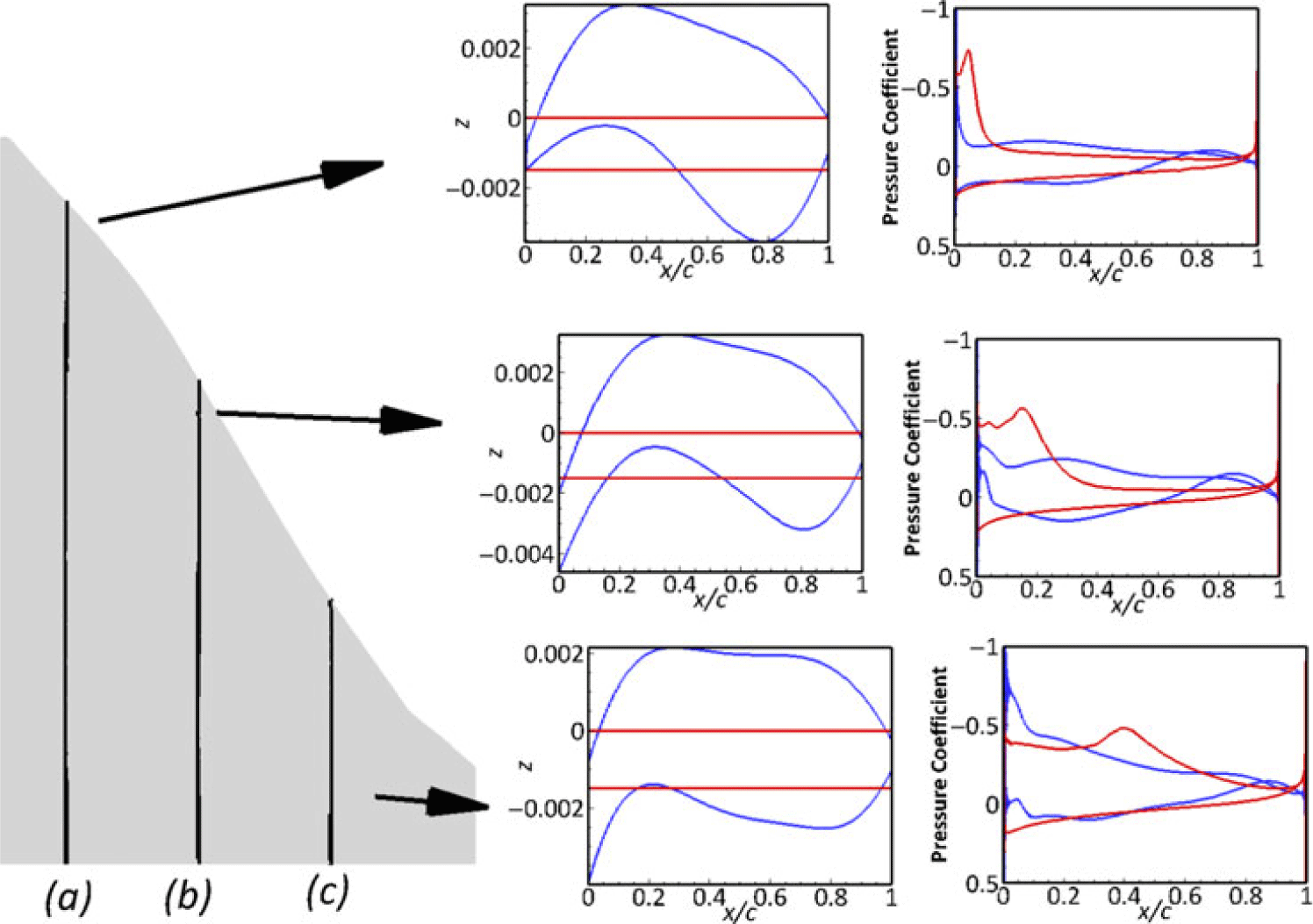
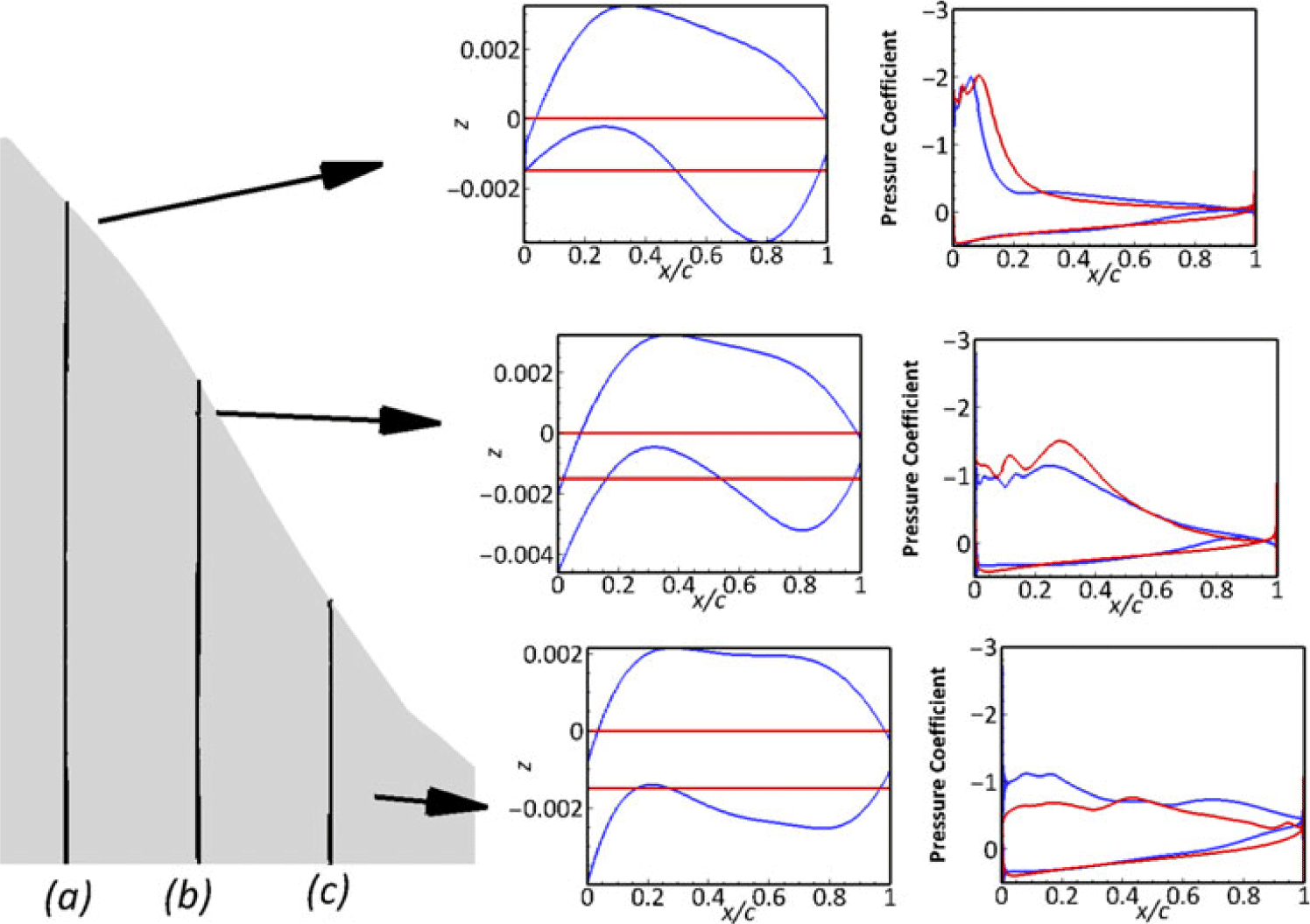
The stream traces on the both upper and lower surfaces of two configuration at α = 4deg and 14deg are shown in Figs. 8(a)–(d). There is no separation at both sides for the initial geometry due to the small angle-of-attack, however, a small back-flow region can be observed in the lower surface of optimised geometry due to the chamber of the leading edge. Considering the profile changes demonstrated in Figs. 9 and 10 — the separation induced by adverse-pressure-gradient on the upper of winglet has been eliminated — this improvement can be regarded as the main reason for drag reduction, which will reduce the strength of wing-tip vortices. The leading-edge separation at the large angle, which is shown in Fig. 8(c), has been removed with the changing of profiles of the main wing. Meanwhile, the development of stall that can be concluded from the separation change is from tip to root in the optimised configuration. However, the baseline geometry leads to a unified separation along the leading edge to trailing edge; this is pernicious for the manoeuvering stability if the airplane has a large angle-of-attack because the separation reduce the controllability of the control surface.
Optimisation for the profiles. (a) Baseline. (b) Optimization.(c) Baseline (d) Optimization.

Comparison of profiles and surface pressure coefficient at the locations of y = 0.02m, 0.06m and 0.1m(
 $\alpha $
= 4deg).

Comparison of profiles and surface pressure coefficient at the locations of y = 0.02m, 0.06m and 0.1m(
 $\alpha $
= 14deg).

3.3 Effects of winglet and leading-edge line type
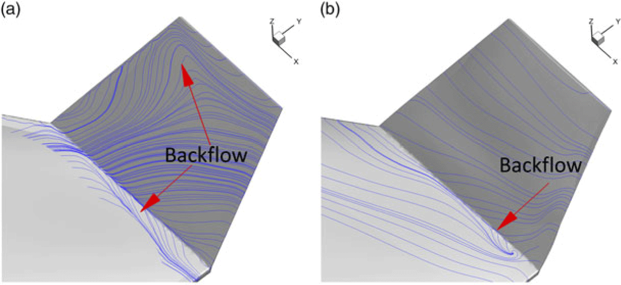
The winglet may be regarded as an efficient device to reduce the drag induced by wing-tip vortices. Figures 11(a) and (b) presents the details of flow field on the winglet. A backflow region occupies the first half of the winglet; the manoeuverable capability could be decreased.
The stream traces on winglet of different model at 4deg. (a) Baseline (b) Optimization.

The optimised solver increases the chamber of the winglet to obtain a large delay stall AoA. The backflow region is eliminated from the baseline, and moreover, the separation at the junction of wing and winglet is shrunk by the variation of the profile of the winglet.
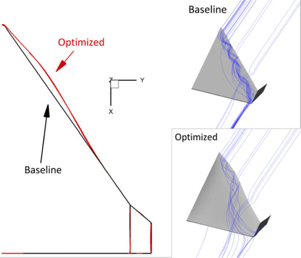
The line type of the leading edge is enlarged on the optimised model, and this change makes the new model a dual-delta-wing configuration. The path lines shown in Fig. 12 show that a detached vortex tube develops from the tail to the out section of the wing on the baseline, and correspondingly, the direction of the vortex tube slightly deflects to the center plane of the wing, which will enhance the ability of boundary layer in the main wing to resist the adverse pressure gradient.
Comparison of line type of leading edge and near-wall path lines at
 $\alpha $
= 14deg.

Comparison between the baseline and optimised model

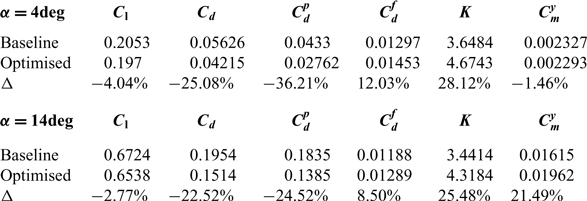
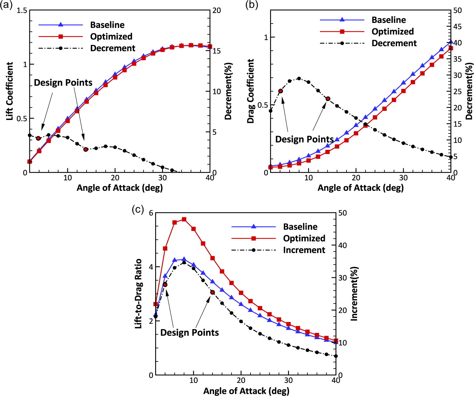
Based on the configuration optimised by the former section, the forces from the optimised winglet and leading-edge line type is presented in a set of plots in Figs. 13(a)–(c), corresponding to lift, drag and lift-to-drag ratio. Fig. 13(a) shows a slight lift dropping for the whole AoA range. Nevertheless, no more than 5% lift loss in Fig. 13(a) can be neglected, if compared with a 25% and 22.5% drag reduction at both design points plotted in Figs. 13(b) and (c), which shows the change of the lift-to-drag ratio with the AoA. Between two design points, the maximum lift-to-drag ratio increases by 32% at 10deg. The detail aerodynamic force of baseline and optimised models is given in the Table 1.
Optimisation for the winglet and leading-edge line type. (a) Lift curve. (b) Drag curve (c) Lift-to-drag ratio

4.0 CONCLUSION
Optimisation performed using an objective function based on a weighted integral is an effective technique for design over multiple operating conditions. The aerodynamic performance was optimised with an adjoint-based method. The rectangle profile was optimised to be a low-speed airfoil, and the separation at winglet was removed by varying the winglet profile. The detached vortex, which was regarded as a positive flow field to enlarge the stall angle, was deflected reasonably to induce the high-momentum flow to the near-wall region of main wing. The lift-to-drag ratio of the configuration is significantly improved by increasing lift and decreasing drag, and correspondingly the aerodynamic performance is improved. Meanwhile, the applicability of this method to aerodynamic shape optimisation under low Reynolds number is also verified.
ACKNOWLEDGEMENTS
The authors acknowledge the support from China Postdoctoral Science Foundation (Grant No. 2017M623184). The computation support comes from Beijing Super Cloud Computing Center and is also acknowledged.