








1. Introduction
1.1. Considered problem, context, and motivation
This paper is concerned with the following constrained nonlinear Schrödinger–Newton system with a point interaction:
 \begin{equation}
\begin{cases}
- \Delta_\alpha u + \omega u
=
w u
+
\beta u \lvert u\rvert^{p - 2}
&\text{on} ~ \mathbb{R}^2;
\\
- \Delta w = 2 \pi \lvert u\rvert^2
&\text{on} ~ \mathbb{R}^2;
\\
\lVert u\rVert_{L^2}^2 = c,
\end{cases}
\end{equation}
where  $p \gt 2$;
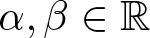
 $\alpha, \beta \in \mathbb{R}$;
 $c \gt 0$;
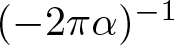
 $- \Delta_\alpha$ denotes the Laplacian of point interaction with s-wave scattering length
 $(- 2 \pi \alpha)^{- 1}$; the unknowns being
 $u \colon \mathbb{R}^2 \to \mathbb{C}$,
 $w \colon \mathbb{R}^2 \to \lbrack0, \infty\lbrack$ and the Lagrange multiplier
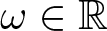
 $\omega \in \mathbb{R}$.
Let us briefly recall what we mean by s-wave scattering length. It is classical that we can decompose the space of square-integrable functions on  $\mathbb{R}^2$ as the tensor product of the space of radial square-integrable functions and the space of square-integrable functions on the circle,
 \begin{equation*}
L^2 (\mathbb{R}^2)
\simeq
L^2 (\rbrack0, \infty\lbrack, r \mathrm{d} r)
\otimes
L^2 (\mathbb{S}^1).
\end{equation*}
The space  $L^2 (\mathbb{S}^1)$ can be further decomposed in terms of circular harmonics:
 \begin{equation*}
L^2 (\mathbb{S}^1)
=
\bigoplus_{m \in \mathbb{Z}} \mathrm{span} \{Y_m\},
\quad \text{where} \quad
Y_m (z)
:=
\frac{1}{\sqrt{2 \pi}} e^{\mathrm{i} m z}.
\end{equation*}
With respect to this decomposition, the Laplacian of point interaction will only differ from the usual Laplacian on the space generated by the s-wave  $Y_0$. In this context, the s-wave scattering length
 $
\ell_\alpha
=
(- 2 \pi \alpha)^{- 1}
=
\frac{\tan \delta_\alpha (k)}{k}
$ provides a measure of how the action of the Laplacian of point interaction affects s-waves, where
 $\delta_\alpha (k)$ denotes the phase shift of an s-wave with angular wavenumber
 $k$.
We proceed to a comment on what we mean by a point interaction. We let  $\{-\overset{\circ}{\Delta}_\alpha\}_{\alpha \in \rbrack-\infty,\infty\rbrack}$, denote the family of
 $L^2$-self-adjoint extensions of the closure of the operator
 $
- \Delta|_{C_0^\infty (\mathbb{R}^2 \setminus \{0\})}
$. This definition provides a family of
 $L^2$-self-adjoint operators that model the behaviour of a potential concentrated at the origin. Different from the one-dimensional delta-interaction, this procedure on
 $\mathbb{R}^2$ relies on suitable renormalization that connects the parameter
 $\alpha$ to the scattering length
 $(- 2 \pi \alpha)^{- 1}$, while the similar parameter on
 $\mathbb{R}$ actually plays the role of a coupling constant. In this paper, we deviate from the usual notation for technical reasons and we understand the Laplacian of point interaction to be the operator
 $- \Delta_\alpha$ obtained as a natural extension of
 $- \overset{\circ}{\Delta}_\alpha$ to a certain linear subspace of
 $L^2_{\mathrm{loc}}$. For more details, see Section 1.3.
In order to motivate our analysis, we first consider the following system:
 \begin{equation}
\begin{cases}
- \Delta u + \omega u
=
w u
+
\beta u \lvert u\rvert^{p - 2}
&\text{in} ~ \mathbb{R}^N;
\\
- \Delta w = C_N \lvert u\rvert^2
&\text{in} ~ \mathbb{R}^N,
\end{cases}
\end{equation}
where
 \begin{equation*}
C_N
:=
\begin{cases}
2 \pi,
&\text{if} ~ N = 2;
\\
N (N - 2) L_N,
&\text{if} ~ N \geq 3;
\end{cases}
\end{equation*}
 $L_N$ denotes the Lebesgue measure of the unit ball in
 $\mathbb{R}^N$ and we want to solve for
 $u \colon \mathbb{R}^N \to \mathbb{C}$,
 $w \colon \mathbb{R}^N \to \lbrack0, \infty\lbrack$ and
 $\omega \in \mathbb{R}$. The usual approach to study (1.2) involves considering the fundamental solution of
 $-\Delta$, that is, the function
 $
\Phi_N
\colon
\mathbb{R}^N \setminus \{0\} \to \mathbb{R}
$ defined as
 \begin{equation*}
\Phi_N (x)
=
\begin{cases}
-\frac{1}{2 \pi}
\log \lvert x\rvert,
&\text{if} ~ N = 2;
\\
\frac{1}{C_N \lvert x\rvert^{N - 2}},
&\text{if} ~ N \geq 3.
\end{cases}
\end{equation*}
The identity  $- \Delta \Phi_N = \delta_0$ holds in the sense of distributions, so the function
 \begin{equation*}
w_u
:=
C_N
\Phi_N \ast \lvert u\rvert^2
=
C_N
\int
\Phi_N (\cdot - y)
\lvert u (y)\rvert^2
\mathrm{d} y
\end{equation*}
formally satisfies  $- \Delta w_u = C_N \lvert u\rvert^2$. As such, we turn our attention to the integrodifferential equation that follows, which corresponds to a Schrödinger equation with mixed nonlocal (convolution-type) and local (pure-power) nonlinearities:
 \begin{equation}
- \Delta u + \omega u
=
w_u u + \beta u \lvert u\rvert^{p - 2}
\quad \text{in} \quad \mathbb{R}^N.
\end{equation}
At least formally, (1.3) is associated with the energy functional
 \begin{equation}
\mathcal{E} (u)
:=
\int_{\mathbb{R}^N}
\frac{1}{2}
\lvert\nabla u (x)\rvert^2
-
\frac{1}{4}
w_u (x)
\lvert u (x)\rvert^2
-
\frac{\beta}{p}
\lvert u (x)\rvert^p
\mathrm{d} x.
\end{equation}
When  $N = 3$ and
 $\beta = 0$, (1.3) models the spatial profile of standing waves of quantum matter with energy
 $\omega$ under the sole effect of a nonlocal self-attractive interaction, appearing in numerous physical contexts (see [Reference Lieb19, Reference Pekar28, Reference Penrose29]).
On one hand, (1.3) has already been widely studied when  $N \geq 3$ and
 $2 \leq p \leq 2 N / (N - 2)$, in which case it follows from the Hardy–Littlewood–Sobolev inequality and the Sobolev embeddings that
 $\mathcal{E}$ is well defined in the usual Sobolev space
 $W^{1, 2} (\mathbb{R}^N)$. We refer the reader to Moroz & Van Schaftingen [Reference Moroz and Van Schaftingen26, Reference Moroz and Van Schaftingen27] for an overview of the current knowledge about this problem when
 $N \geq 3$.
On the other hand, the literature concerned with (1.3) is scarcer in the more mathematically challenging case  $N = 2$. For instance, the nonlinear functional obtained by the formal mapping
 \begin{equation*}
u
\mapsto
\int
\lvert\nabla u (x)\rvert^2
+
\log (\lvert x - y\rvert)
\lvert u (x)\rvert^2
\lvert u (y)\rvert^2
\mathrm{d} x
\end{equation*}
is not nonnegative in this case because the logarithm is sign-changing (unlike the case in higher dimensions with  $\log$ replaced by
 $\Phi_N$). Furthermore, this formal mapping is not well defined in the natural Sobolev space
 $W^{1, 2}$ due to the singularity and unboundedness of the logarithm. In view of these peculiarities and the associated challenge to deal with them, there is an increasing interest and a rapidly expanding literature concerned with this problem. To cite a few papers, we highlight Stubbe [Reference Stubbe30], which introduced a convenient variational framework to treat this problem (see Section 1.4); Masaki [Reference Masaki22], which established the well-posedness of the associated Cauchy problem in the energy space; [Reference Cingolani and Weth12, Reference Miao and Weth23] obtained several existence and multiplicity results; Cingolani & Jeanjean [Reference Cingolani and Jeanjean11] established existence and non-existence results for the normalized problem
 \begin{equation*}
\begin{cases}
- \Delta u = w_u u + \beta u \lvert u\rvert^{p - 2}
&\text{on} ~ \mathbb{R}^2;
\\
\lVert u\rVert_{L^2}^2 = c,
\end{cases}
\end{equation*}
and [Reference Alves, Böer and Miyagaki6, Reference Chen, Radulescu and Tang31] obtained existence and multiplicity results for the normalized problem with an exponential nonlinearity (which corresponds to the Sobolev-critical growth on  $\mathbb{R}^2$ as evidenced by the Trudinger–Moser inequality) in place of the pure power nonlinearity.
We return the focus to (1.1), which is obtained from (1.2) in the case  $N = 2$ by replacing the Laplacian
 $- \Delta$ with the Laplacian of point interaction
 $- \Delta_\alpha$. The model for point interactions considered in this paper was introduced by Berezin & Faddeev in the 1960s (see [Reference Berezin and Faddeev9]) and the standard reference for this subject is Albeverio, Gesztesy, Høegh-Krohn, & Holden’s comprehensive treatise [Reference Albeverio, Gesztesy, Hoegh-Krohn and Holden5], but we also refer the reader to [Reference Albeverio and Figari4, Reference Gallone and Michelangeli17, Reference Michelangeli, Ottolini and Scandone25] for more modern and general treatments. Nonetheless, the study of semilinear nonlocal problems involving a point interaction in dimensions 2 and 3 is much more recent. We proceed to a quick review of the relevant literature. Consider the Hartree equation with a point interaction,
 \begin{equation*}
\mathrm{i} \psi' (t)
=
- \overset{\circ}{\Delta}_\alpha \psi (t)
-
(w \ast \lvert\psi (t)\rvert^2)
\psi (t)
\quad \text{in} \quad
\mathbb{R}^N.
\end{equation*}
In [Reference Michelangeli, Olgiati and Scandone24], Michelangeli, Olgiati, & Scandone obtained results about the well-posedness of the associated Cauchy problem in dimension  $N = 3$ when
 $\alpha \geq 0$ under hypotheses on the integrability of
 $w$. In [Reference Georgiev, Michelangeli and Scandone18], Georgiev, Michelangeli, & Scandone obtained action ground states, their qualitative properties and established the well-posedness for the associated Cauchy problem in dimension
 $N = 2$ when
 $w$ is non-negative, radial, non-increasing and sufficiently integrable. The analogous system to (1.1) obtained when considering self-repulsion instead of self-attraction is the nonlinear Schrödinger–Maxwell system (often called the nonlinear Schrödinger–Poisson system) with a point interaction:
 \begin{equation*}
\begin{cases}
- \overset{\circ}{\Delta}_\alpha u + \omega u + w u
=
\beta u \lvert u\rvert^{p - 2}
&\text{in} ~ \Omega;
\\
- \Delta w = \omega_N \lvert u\rvert^2
&\text{in} ~ \Omega
\end{cases}
\end{equation*}
(for the case  $\alpha = \infty$, the reader may, respectively, find a physical deduction of this system and an investigation of the time-dependent system in [Reference Antonelli, Marcati and Scandone8, Reference d’Avenia15]). The Dirichlet problem where
 $\beta = 0$ and
 $\Omega$ denotes a smooth bounded subset of
 $\mathbb{R}^3$ was considered by Coclite & Holden in [Reference Coclite and Holden13, Reference Coclite and Holden14], where the existence of nontrivial weak solutions and ground states was established. Furthermore, the normalized problem in
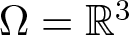 $\Omega = \mathbb{R}^3$ was recently considered in [Reference de Paula Ramos16], where the existence of ground states with sufficiently small mass was established.
In this context, this paper is motivated by the fact that, to the best of our knowledge, there are no studies about the planar nonlinear Schrödinger–Newton system with a point interaction. More precisely, our main goal is to prove the existence of ground states of
 \begin{equation*}
\begin{cases}
- \Delta_\alpha u = w_u u + \beta u \lvert u\rvert^{p - 2}
&\text{on} ~ \mathbb{R}^2;
\\
\lVert u\rVert_{L^2}^2 = c,
\end{cases}
\end{equation*}
(see Theorem 1.5).
We finish with a comment on the organization of the rest of the introduction.
• In Section 1.2, we fix the notation used throughout the paper.
• In Section 1.3, we recall the precise definition of
 $- \Delta_\alpha$.
• In Section 1.4, we introduce the relevant variational framework.
• In Section 1.5, we state our main results.

1.2. Notation
• We integrate over the entire plane
$\mathbb{R}^2$ when the domain of integration is omitted.• The open ball on
$\mathbb{R}^2$ centred at
$x$ with radius
$r \gt 0$ is denoted by
$B_r (x)$.• Unless denoted otherwise, we consider complex functional spaces of functions defined a.e. on
$\mathbb{R}^2$. Nonlinear functionals on these spaces are denoted by uppercase calligraphic Latin letters
$\mathcal{A}, \mathcal{B}, \mathcal{C} \ldots$• Sesquilinear forms are linear in the second entry and we enclose their argument with square brackets. In the case of inner products, we most often employ the conventional notation
$\langle\cdot, \cdot\rangle$.• The Sobolev space
$W^{k, p}$ (resp., homogeneous Sobolev space
$\dot{W}^{k, p}$) contains a.e.-defined functions whose weak derivatives of order
$0, \ldots, k$ (resp., of order
$k$) are in
$L^p$.• If
$X$ is a Hilbert space, then we denote its topological-linear dual by
$X^*$ and the following notation is employed for the real part of the duality pairing:
\begin{equation*}
\langle T, x\rangle_{X^*, X}
:=
\Re (T x)
\end{equation*}for every
$T \in X^*$ and
$x \in X$.


1.3. The Laplacian of point interaction
1.3.1. Definition
We need to introduce a family of Green’s functions to rigorously define the Laplacian of point interaction. Let  $
G_\lambda
\colon
\mathbb{R}^2 \setminus \{0\}
\to
\rbrack0, \infty\lbrack
$ be given by
 \begin{equation*}
G_\lambda (x)
=
\frac{1}{2 \pi}
K_0 (\sqrt{\lambda} \lvert x\rvert),
\end{equation*}
so that  $
- \Delta G_\lambda + \lambda G_\lambda
=
\delta_0
$ in the sense of distributions, where
 $K_0$ denotes a modified Bessel function of the second kind (see [Reference Abramowitz and Stegun1, Section 9.6]). Green’s function
 $G_\lambda$ has exponential decay at infinity and
 \begin{equation*}
\frac{G_\lambda (x)}
{
- \frac{\log (\sqrt{\lambda} \lvert x\rvert)}{2 \pi}
}
\xrightarrow[x \to 0]{}
1,
\end{equation*}
so
 \begin{equation}
G_\lambda \in L^r
\quad \text{for every} \quad
r \in \lbrack2, \infty\lbrack.
\end{equation}
Following [Reference Albeverio, Gesztesy, Hoegh-Krohn and Holden5, Chapter I.5], the self-adjoint operator  $- \overset{\circ}{\Delta}_\alpha \colon \operatorname{Dom} (- \overset{\circ}{\Delta}_\alpha) \to L^2$ is defined as
 \begin{equation*}
- \overset{\circ}{\Delta}_\alpha u = - \Delta \phi - q \lambda G_\lambda
\end{equation*}
for every  $
u
=
\phi + q G_\lambda \in \operatorname{Dom} (- \overset{\circ}{\Delta}_\alpha)
$, where
 \begin{equation}
\operatorname{Dom} (- \overset{\circ}{\Delta}_\alpha)
:=
\{
\phi + q G_\lambda:
\phi \in W^{2, 2}, ~
q \in \mathbb{C}, ~
\lambda \gt 0
\quad \text{and} \quad
(\alpha + \theta_\lambda) q
=
\phi (0)
\},
\end{equation}
 \begin{equation*}
\theta_\lambda
:=
\frac{\gamma}{2 \pi}
+
\frac{1}{2 \pi}
\log (\frac{\sqrt{\lambda}}{2})
\end{equation*}
and
 \begin{equation*}
\gamma
:=
\lim_{n \to \infty} (
-
\log n
+
\sum_{1 \leq k \leq n} \frac{1}{k}
)
\in \rbrack0.57, 0.58\lbrack
\end{equation*}
is the Euler–Mascheroni constant.
1.3.2. Nonuniqueness of decomposition
An important aspect of  $\operatorname{Dom} (- \overset{\circ}{\Delta}_\alpha)$ is the nonuniqueness of decomposition of its elements. More precisely, consider the set
 \begin{equation*}
D
:=
\{
\phi + q G_\lambda :
\phi \in W^{1, 2}_\mathrm{loc}, \quad
q \in \mathbb{C}
\quad \text{and} \quad
\lambda \gt 0
\},
\end{equation*}
which clearly contains  $\operatorname{Dom} (- \overset{\circ}{\Delta}_\alpha)$. The fact that we consider functions on the more general local Sobolev space
 $W^{1, 2}_\mathrm{loc}$ instead of the standard Sobolev space
 $W^{1, 2}$ will be important later on, and is related to the behaviour of
 $w_u$ at infinity (see Lemma 2.2).
By nonuniqueness of decomposition, we mean the result stated below.
(1) Given
$u \in D$, there exists a unique complex number
$\mathcal{Q} (u)$ (called the charge of
$u$) for which if
$\phi \in W^{1, 2}_\mathrm{loc}$,
$q \in \mathbb{C}$ and
$\lambda \gt 0$ are such that
$u = \phi + q G_\lambda$, then
$q = \mathcal{Q} (u)$.(2) Given
$u \in D$ and
$\lambda \gt 0$, there exists a unique
$\phi_\lambda \in W^{1, 2}_\mathrm{loc}$ such that
$u = \phi_\lambda + \mathcal{Q} (u) G_\lambda$.


The aforementioned nonuniqueness of decomposition stems from the second conclusion in the proposition, which is not a mere statement of uniqueness. In fact, it shows that given  $u \in D$, there exists a continuum of decompositions of
 $u$ indexed by the parameter
 $\lambda \gt 0$, i.e., there exists a unique association
 \begin{equation*}
\rbrack0, \infty\lbrack \ni \lambda \mapsto \phi_\lambda \in W^{1, 2}_\mathrm{loc}
\end{equation*}
such that the equality  $u = \phi_\lambda + \mathcal{Q} (u) G_\lambda$ holds for every
 $\lambda \gt 0$. In brief, this result follows from the fact that if
 $\lambda_1 \neq \lambda_2$, then
 $G_{\lambda_1}-G_{\lambda_2} \in W^{2, 2}$ (see [Reference de Paula Ramos16, Lemma 2.1] for the result in
 $\mathbb{R}^3$, while the proof on
 $\mathbb{R}^2$ is analogous).
1.3.3. The associated energy space
As described in [Reference Albeverio, Gesztesy, Hoegh-Krohn and Holden5, Theorem 5.4], the spectrum of  $- \overset{\circ}{\Delta}_\alpha$ has the form
 \begin{equation*}
\sigma (- \overset{\circ}{\Delta}_\alpha)
=
\sigma_{\text{p}} (- \overset{\circ}{\Delta}_\alpha)
\cup
\sigma_{\text{cont}} (- \overset{\circ}{\Delta}_\alpha),
\end{equation*}
where  $\sigma_{\text{p}} (- \overset{\circ}{\Delta}_\alpha) = \{- \omega_\alpha\}$,
 $\sigma_{\text{cont}} (- \overset{\circ}{\Delta}_\alpha) = \lbrack0, \infty\lbrack$ and
 $
\omega_\alpha
:=
4 e^{- 4 \pi \alpha - 2 \gamma} \gt 0
$. Moreover,
 $- \omega_\alpha$ is the unique eigenvalue of
 $- \overset{\circ}{\Delta}_\alpha$ (moreover, it is a simple eigenvalue). In particular, we obtain the following inner product on
 $\operatorname{Dom} (- \overset{\circ}{\Delta}_\alpha)$:
 \begin{equation}
(u, v)
\mapsto
\langle- \overset{\circ}{\Delta}_\alpha u, v\rangle_{L^2}
+
(1 + \omega_\alpha)
\langle u, v\rangle_{L^2}.
\end{equation}
We define  $W^{1, 2}_\alpha$ as the Hilbert space obtained as completion of
 $\operatorname{Dom} (- \overset{\circ}{\Delta}_\alpha)$ with respect to (1.7) and we call
 $W^{1, 2}_\alpha$ the energy space associated with
 $- \overset{\circ}{\Delta}_\alpha$.
The underlying vector space of  $W^{1, 2}_\alpha$ is often called the form domain of
 $- \overset{\circ}{\Delta}_\alpha$ and is explicitly given by
 \begin{equation}
\operatorname{Dom} \lbrack- \overset{\circ}{\Delta}_\alpha\rbrack
:=
\{
\phi + q G_\lambda :
\phi \in W^{1, 2}, \quad
q \in \mathbb{C}
\quad \text{and} \quad
\lambda \gt 0
\}.
\end{equation}
Notice that while there is an expression relating the value of the charge  $q$ and the value
 $\phi (0)$ in the operator domain (1.6), such an expression is absent from the definition of the form domain (1.8). The inner product of
 $W^{1, 2}_\alpha$ is given by
 \begin{equation}
\langle u, v\rangle_{W^{1, 2}_\alpha}
:=
H_\alpha \lbrack u, v\rbrack
+
(1 + \omega_\alpha)
\langle u, v\rangle_{L^2},
\end{equation}
where
 \begin{equation*}
H_\alpha \lbrack u, v\rbrack
:=
\langle\phi_u, \phi_v\rangle_{\dot{W}^{1, 2}}
+
\lambda (
\langle\phi_u, \phi_v\rangle_{L^2}
-
\langle u, v\rangle_{L^2}
)
+
(\alpha + \theta_\lambda)
\overline{q_u} q_v
\end{equation*}
for every  $u = \phi_u + q_u G_\lambda$ and
 $v = \phi_v + q_v G_\lambda$ in
 $\operatorname{Dom} \lbrack- \overset{\circ}{\Delta}_\alpha\rbrack$. More precisely, the Hermitian form
 $H_\alpha$ denotes the unique continuous extension to
 $\operatorname{Dom} \lbrack- \overset{\circ}{\Delta}_\alpha\rbrack$ of
 \begin{equation}
\operatorname{Dom} (- \overset{\circ}{\Delta}_\alpha) \times \operatorname{Dom} (- \overset{\circ}{\Delta}_\alpha)
\ni
(u, v)
\mapsto
\langle- \overset{\circ}{\Delta}_\alpha u, v\rangle_{L^2}.
\end{equation}
(1) For a proof that
$H_\alpha$ is well defined, see [Reference de Paula Ramos16, Lemma 2.4]).(2) The identity
\begin{equation*}
\langle
- \Delta \phi + \lambda \phi,
G_\lambda
\rangle_{L^2}
=
\phi (0)
\end{equation*}for every
$\lambda \gt 0$ and
$\phi \in W^{2, 2}$ (see Lemma 2.1) is essential to prove that
$H_\alpha$ extends the Hermitian form (1.10). For an analogous identity in
$\mathbb{R}^3$, see [Reference de Paula Ramos16, Lemma 2.3].


For notational reasons, it will be useful to define the nonlinear functional (Instead of the term nonlinear functional, many texts concerned with similar problems use the term quadratic form (see [Reference Gallone and Michelangeli17], for instance). We opted to avoid this terminology because there are nonequivalent definitions of ‘quadratic forms’ in the literature. Nonetheless, the more generic term ‘nonlinear functional’ always seems to apply.)  $\mathcal{H}_\alpha \colon W^{1, 2}_\alpha \to \mathbb{R}$ as
 \begin{equation}
\mathcal{H}_\alpha (u)
=
H_\alpha \lbrack u, u\rbrack
=
\lVert\phi\rVert_{\dot{W}^{1, 2}}^2
+
\lambda (
\lVert\phi\rVert_{L^2}^2
-
\lVert u\rVert_{L^2}^2
)
+
(\alpha + \theta_\lambda)
\lvert q\rvert^2
\end{equation}
for every  $u = \phi + q G_\lambda \in \operatorname{Dom} \lbrack- \overset{\circ}{\Delta}_\alpha\rbrack$. To finish, we highlight that
 $W^{1, 2}_\alpha \hookrightarrow L^r$ for every
 $r \in \lbrack2, \infty\lbrack$. Indeed, it is well known that the Sobolev space
 $W^{1, 2}$ is continuously embedded in
 $L^r$ for every
 $r \in \lbrack2, \infty\lbrack$. In view of the integrability properties of
 $G_\lambda$ in (1.5), the expression of the form space
 $\operatorname{Dom} \lbrack- \overset{\circ}{\Delta}_\alpha\rbrack$ in (1.8) and the inner product of
 $W^{1, 2}_\alpha$ in (1.9), we deduce that the analogous embeddings hold for
 $W^{1, 2}_\alpha$.
1.3.4. An extension of the Laplacian of point interaction
Consider the natural extension of  $- \overset{\circ}{\Delta}_\alpha$ obtained as follows: let the linear operator
 $- \Delta_\alpha \colon \operatorname{Dom} (- \Delta_\alpha) \to L^2_{\mathrm{loc}}$ be defined by mapping
 $u = \phi + q G_\lambda \in \operatorname{Dom} (- \Delta_\alpha)$ to
 \begin{equation*}- \Delta_\alpha u = - \Delta \phi - q \lambda G_\lambda,\end{equation*}
where
 \begin{equation*}
\operatorname{Dom} (- \Delta_\alpha)
:=
\{
\phi + q G_\lambda:
\phi \in W^{2, 2}_{\mathrm{loc}}, ~
\lambda \gt 0
\quad \text{and} \quad
(\alpha + \theta_\lambda) q
=
\phi (0)
\}.
\end{equation*}
In Section 1.5, we comment on the motivation for considering this extension.
1.4. Variational framework
The strategy adopted in Stubbe [Reference Stubbe30] to obtain a functional space where (1.4) is well defined consisted of introducing the Hilbert space  $
X := (
\mathrm{VS} (X), \langle\cdot, \cdot\rangle_X
)
$, where
 \begin{equation*}
\mathrm{VS} (X)
:=
\left\{
\phi \in W^{1, 2}:
\int
\log (1 + \lvert x\rvert)
\lvert\phi (x)\rvert^2
\mathrm{d} x \lt \infty
\right\}
\end{equation*}
and
 \begin{equation*}
\langle\phi, \psi\rangle_X
:=
\langle\phi, \psi\rangle_{W^{1, 2}}
+
\int
\log (1 + \lvert x\rvert)
\overline{\phi (x)}
\psi (x)
\mathrm{d} x.
\end{equation*}
Let us briefly explain why  $\mathcal{E}$ is well defined on
 $X$. Elementary computations show that
 \begin{equation*}
\log t
=
\log (1 + t)
-
\log \left(1 + \frac{1}{t}\right)
\end{equation*}
for every  $t \gt 0$. In particular,
 \begin{multline*}
\int \int
\log (\lvert x - y\rvert)
\lvert\phi (x)\rvert^2
\lvert\phi (y)\rvert^2
\mathrm{d} x \mathrm{d} y
=
\\
\begin{aligned}
&=
\int \int
\log (1 + \lvert x - y\rvert)
\lvert\phi (x)\rvert^2
\lvert\phi (y)\rvert^2
\mathrm{d} x \mathrm{d} y
\\
&-
\int \int
\log \left(1 + \frac{1}{\lvert x - y\rvert}\right)
\lvert\phi (x)\rvert^2
\lvert\phi (y)\rvert^2
\mathrm{d} x \mathrm{d} y.
\end{aligned}
\end{multline*}
On one hand, the first integral on the RHS is well defined due to the definition of  $X$. On the other hand, the second integral on the RHS is also well defined due to the elementary inequality
 \begin{equation*}
\log \left(1 + \frac{1}{t}\right)
\leq
\frac{1}{t}
\end{equation*}
for every  $t \gt 0$ and the Hardy–Littlewood–Sobolev inequality (see Proposition 3.6).
Inspired by this construction, we introduce the Hilbert space  $
X_\alpha
:=
(
\mathrm{VS} (X_\alpha),
\langle\cdot, \cdot\rangle_{X_\alpha}
)
$, where
 \begin{equation*}
\mathrm{VS} (X_\alpha)
:=
\left\{
u \in W^{1, 2}_\alpha:
\int
\log (1 + \lvert x\rvert)
\lvert u (x)\rvert^2
\mathrm{d} x \lt \infty
\right\}
\end{equation*}
and
 \begin{equation*}
\langle u, v\rangle_{X_\alpha}
:=
\langle u, v\rangle_{W^{1, 2}_\alpha}
+
\int
\log (1 + \lvert x\rvert)
\overline{u (x)}
v (x)
\mathrm{d} x.
\end{equation*}
Remark 1.3. Equivalently,
 \begin{equation*}
\mathrm{VS} (X_\alpha)
=
\{
\phi + q G_\lambda:
\phi \in X, \quad
q \in \mathbb{C}
\quad and \quad
\lambda \gt 0
\}
\end{equation*}
because Green’s function  $G_\lambda$ is square-integrable and has exponential decay at infinity, so
 $
\int
\log (1 + \lvert x\rvert)
G_\lambda (x)^2
\mathrm{d} x \lt \infty
$.
As such, we naturally associate the integrodifferential equation
 \begin{equation*}- \Delta_\alpha u = w_u u + \beta u \lvert u\rvert^{p - 2}\end{equation*}
with the energy functional  $\mathcal{E}_\alpha \colon X_\alpha \to \mathbb{R}$ defined as
 \begin{equation}
\mathcal{E}_\alpha (u)
=
\frac{1}{2}
\mathcal{H}_\alpha (u)
+
\frac{1}{4}
\mathcal{V}_0 (u)
-
\frac{\beta}{p}
\mathcal{C} (u),
\end{equation}
where
 \begin{equation*}
\mathcal{V}_0 (u)
:=
\int \int
\log (\lvert x - y\rvert)
\lvert u (x)\rvert^2
\lvert u (y)\rvert^2
\mathrm{d} x \mathrm{d} y
\end{equation*}
and  $\mathcal{C} (u) := \lVert u\rVert_{L^p}^p$. Inspired by [Reference Cingolani and Jeanjean11, Reference Cingolani and Weth12], we also define the nonlinear functionals
 $\mathcal{V}_1 \colon X_\alpha \to \lbrack0, \infty\lbrack$,
 $\mathcal{V}_2 \colon L^{\frac{8}{3}} \to \lbrack0, \infty\lbrack$ as given by
 \begin{equation}
\mathcal{V}_1 (u)
=
\int \int
\log (1 + \lvert x - y\rvert)
\lvert u (x)\rvert^2
\lvert u (y)\rvert^2
\mathrm{d} x \mathrm{d} y
\end{equation}
and
 \begin{equation}
\mathcal{V}_2 (u)
=
\int \int
\log \left(1 + \frac{1}{\lvert x - y\rvert}\right)
\lvert u (x)\rvert^2
\lvert u (y)\rvert^2
\mathrm{d} x \mathrm{d} y,
\end{equation}
so that  $\mathcal{V}_0 = \mathcal{V}_1 - \mathcal{V}_2$ in
 $X_\alpha$. To finish, we highlight a few results that follow from the arguments in the proof of [Reference Cingolani and Weth12, Lemma 2.2].
(1) The Hilbert space
$X_\alpha$ is compactly embedded in
$L^r$ for every
$r \in \lbrack2, \infty\lbrack$.(2) If
$\{u_n\}_{n \in \mathbb{N} \cup \{\infty\}} \subset X_\alpha$ is such that
$u_n \rightharpoonup u_\infty$ in
$W^{1, 2}_\alpha$ as
$n \to \infty$, then
$
\mathcal{V}_1 (u_\infty)
\leq
\liminf_{n \to \infty} \mathcal{V}_1 (u_n)
$.(3) The energy functional
$\mathcal{E}_\alpha$ is of class
$C^1$. Moreover, its derivative is computed as
\begin{align*}
\bigg\langle\mathcal{E}_\alpha' (u), v\bigg\rangle_{X_\alpha^*, X_\alpha}
&=
H_\alpha \lbrack u, v\rbrack
\\
&+
\Re \left(
\int \int
\log (\lvert x - y\rvert)
\lvert u (x)\rvert^2
\overline{u (x)} v (x)
\mathrm{d} x \mathrm{d} y
\right)
\\
&-
\beta
\Re \left(
\int
\lvert u (x)\rvert^{p - 2}
\overline{u (x)} v (x)
\mathrm{d} x
\right)
\end{align*}for every
$u, v \in X_\alpha$.


1.5. Main results
Our first result establishes sufficient conditions for the existence of ground states of (1.1), i.e., solutions to the following minimization problem:
 \begin{equation}
\begin{cases}
\mathcal{E}_\alpha (u)
=
m_\alpha (c)
:=
\inf_{v \in \mathscr{S}_\alpha (c)} \mathcal{E}_\alpha (v);
\\
u \in \mathscr{S}_\alpha (c),
\end{cases}
\end{equation}
where  $
\mathscr{S}_\alpha (c)
:=
\{u \in X_\alpha: \lVert u\rVert_{L^2}^2 = c\}
$.
Theorem 1.5. Suppose that  $\alpha \in \mathbb{R}$,
 $c \gt 0$ and one of the following conditions is satisfied:
(1)
$\beta \leq 0$ and
$p \gt 2$;(2)
$\beta \gt 0$ and
$2 \lt p \lt 4$;(3)
$\beta \gt 0$,
$p = 4$ and
$
c \lt 2 / (
\beta \widetilde{K}_{\mathrm{GN}} (p)
)
$,


where  $\widetilde{K}_{\mathrm{GN}} (p)$ denotes the positive constant for which the Gagliardo–Nirenberg inequality in Proposition 3.7 holds. The following implications are satisfied.


The general argument used to prove the theorem follows the ideas in Cingolani & Jeanjean [Reference Cingolani and Jeanjean11]. In view of the presence of the point interaction, this paper considers a problem that is not invariant by translation. As such, we do not obtain a convergent sequence of the form  $(u_n (\cdot - x_n))_{n \in \mathbb{N}}$ as in [Reference Cingolani and Jeanjean11, Theorem 1.1]. Notice that this is coherent with the fact that the Hilbert space
 $X_\alpha$ does not contain translates of functions in
 $X_\alpha \setminus X$.
Let us sketch the main difference with the arguments used to prove [Reference Cingolani and Jeanjean11, Theorem 1.1]. Suppose that  $(u_n)_{n \in \mathbb{N}}$ is a minimizing sequence of
 $\mathcal{E}_\alpha|_{\mathscr{S}_\alpha (c)}$. As in Adami, Boni, Carlone, & Tentarelli [Reference Adami, Boni, Carlone and Tentarelli2, Reference Adami, Boni, Carlone and Tentarelli3], the first key point is that (1.15) is energetically convenient with respect to the corresponding problem in the absence of a point interaction, that is,
 \begin{equation}
\begin{cases}
\mathcal{E} (\phi)
=
m (c)
:=
\inf_{\psi \in \mathscr{S} (c)}
\mathcal{E} (\psi);
\\
\phi \in \mathscr{S} (c),
\end{cases}
\end{equation}
where  $
\mathscr{S} (c)
:=
\{\phi \in X: \lVert\phi\rVert_{L^2}^2 = c\}
$ (see Lemma 3.1). In particular, it follows that
 \begin{equation}
\liminf_{n \to \infty}
\lvert\mathcal{Q} (u_n)\rvert \gt 0.
\end{equation}
With an argument reminiscent of the proof of Lions’ concentration-compactness lemma [Reference Lions21, Lemma I.1], we obtain a set  $\{x_n\}_{n \in \mathbb{N}} \subset \mathbb{R}^2$ such that
 $(u_n (\cdot - x_n))_{n \in \mathbb{N}}$ is relatively compact in
 $L^2$. On the other hand, the sequence
 $(u_n (\cdot - x_n))_{n \in \mathbb{N}}$ only stays in
 $X_\alpha$ when either
 $\{u_n\}_{n \in \mathbb{N}} \subset X$ or
 $
\{x_n\}_{n \in \mathbb{N}} = \{0\} \subset \mathbb{R}^2
$. Due to (1.17), we cannot expect the inclusion
 $\{u_n\}_{n \in \mathbb{N}} \subset X$ to hold. Bounded sequences in
 $\mathbb{R}^2$ are relatively compact, so either
 $\{x_n\}_{n \in \mathbb{N}}$ has a divergent subsequence or
 $(u_n)_{n \in \mathbb{N}}$ is relatively compact in
 $L^2$. In the proof of Lemma 3.3, we show that the divergence
 $\lvert x_n\rvert \to \infty$ as
 $n \to \infty$ contradicts (1.17), hence the relative compactness of
 $(u_n)_{n \in \mathbb{N}}$ in
 $L^2$. The rest of the proof follows Cingolani & Jeanjean’s method.
Before proceeding to the next main result, let us comment on the motivation for considering the extension of  $- \overset{\circ}{\Delta}_\alpha$ introduced in Section 1.3.4. Earlier investigations of nonlinear elliptic equations involving a point interaction used the fact that if
 $u = \phi + q G_\lambda$ is a critical point of an energy functional
 $W^{1, 2}_\alpha \to \mathbb{R}$, then
 $u \in \operatorname{Dom} (- \overset{\circ}{\Delta}_\alpha)$ (see [Reference Adami, Boni, Carlone and Tentarelli2, Reference Adami, Boni, Carlone and Tentarelli3, Reference de Paula Ramos16, Reference Georgiev, Michelangeli and Scandone18], for instance). The usual argument to ensure this gain of regularity involves using the fact that if
 $u = \phi + \mathcal{Q} (u) G_\lambda \in W^{1, 2}_\alpha$ is a weak solution to
 $- \Delta_\alpha u = f$ with
 $f \in L^2$, then
 $\phi \in W^{2, 2}$. It is hard to evaluate the applicability of this argument for weak solutions to (1.1) because
 $w_u$ diverges at infinity (see Lemma 2.2), so it is not clear whether
 $w_u u \in L^2$. In this context, we consider an extension of
 $- \overset{\circ}{\Delta}_\alpha$ to a subspace of
 $L^2_{\mathrm{loc}}$ in order to deal with the challenge of the possible divergence
 $\int \lvert\Delta \phi (x)\rvert^2 \mathrm{d} x = \infty$. The next result shows that this approach is successful at a certain degree because we can at least prove that the critical points of
 $\mathcal{E}_\alpha|_{\mathscr{S}_\alpha (c)}$ are automatically in
 $\operatorname{Dom} (- \Delta_\alpha)$, i.e., their regular component is in
 $W^{2, 2}_\mathrm{loc}$.
In fact, our last result is that the critical points of  $\mathcal{E}_\alpha|_{\mathscr{S}_\alpha (c)}$ are naturally associated with standing waves of the evolution equation
 \begin{equation}
\mathrm{i} \psi' (t)
=
- \Delta_\alpha \psi (t)
-
w_{\psi (t)} \psi (t)
-
\beta
\psi (t)
\lvert\psi (t)\rvert^{p - 2}.
\end{equation}
Proposition 1.6. Suppose that  $\alpha \in \mathbb{R}$,
 $p \gt 2$,
 $c \gt 0$,
 $u$ is a critical point of
 $\mathcal{E}_\alpha|_{\mathscr{S}_\alpha (c)}$ and
 $\omega \in \mathbb{R}$ denotes its associated Lagrange multiplier, i.e.,
 \begin{equation}
\bigg\langle
\mathcal{E}_\alpha' (u),
v
\bigg\rangle_{X_\alpha^*, X_\alpha}
+
\omega
\Re \langle u, v\rangle_{L^2}
=
0
\quad \text{for every} \quad
v \in X_\alpha.
\end{equation}
Then  $u \in \operatorname{Dom} (- \Delta_\alpha)$ and the function
 \begin{equation*}
\mathbb{R} \ni t
\mapsto
e^{\mathrm{i} \omega t} u \in \operatorname{Dom} (- \Delta_\alpha)
\end{equation*}
is a standing wave of (1.18) in the sense that
 \begin{equation}
- \Delta_\alpha u + \omega u
=
w_u u
+
\beta u \lvert u\rvert^{p - 2}
\quad \text{a.e. on} \quad
\mathbb{R}^2.
\end{equation}
2. Preliminaries
2.1. Properties of Green’s function
$G_\lambda$

By using the properties of the Fourier transform, an explicit computation shows that
 \begin{equation}
\lVert G_\lambda\rVert_{L^2}^2
=
\frac{1}{4 \pi \lambda}.
\end{equation}
The result that follows is an adaptation of [Reference de Paula Ramos16, Lemma 2.3] to dimension 2.
Lemma 2.1. The following identity is satisfied:
 \begin{equation*}
\int
(- \Delta \phi (x) + \lambda \phi (x))
G_\lambda (x)
\mathrm{d} x
=
\phi (0)
\end{equation*}
for every  $\lambda \gt 0$ and
 $\phi \in W^{2, 2}_{\mathrm{loc}}$.
Proof. It follows from the Chain Rule that
 \begin{equation}
- G_\lambda \Delta \phi
=
- \phi \Delta G_\lambda
+
\mathrm{div} (\phi \nabla G_\lambda - G_\lambda \nabla \phi).
\end{equation}
Consider an  $\varepsilon \gt 0$. Due to (2.2) and the Divergence Theorem [Reference Willem32, Theorem 6.3.5],
 \begin{multline*}
-
\int_{\mathbb{R}^2 \setminus B_\varepsilon (0)}
G_\lambda (x) \Delta \phi (x)
\mathrm{d} x
=
-
\int_{\mathbb{R}^2 \setminus B_\varepsilon (0)}
\phi (x) \Delta G_\lambda (x)
\mathrm{d} x
+
\\
-
\frac{\sqrt{\lambda}}{2 \pi}
K_0' (\sqrt{\lambda} \varepsilon)
\int_{\varepsilon \mathbb{S}^1}
\phi (x)
\mathrm{d} \sigma_\varepsilon (x)
+
\frac{K_0 (\sqrt{\lambda} \varepsilon)}
{2 \pi}
\int_{\varepsilon \mathbb{S}^1}
\frac{\nabla \phi (x) \cdot x}{\lvert x\rvert}
\mathrm{d} \sigma_\varepsilon (x)
\end{multline*}
where  $\sigma_\varepsilon$ denotes the surface measure of
 $\varepsilon \mathbb{S}^1$. A change of variable shows that
 \begin{multline*}
-
\int_{\mathbb{R}^2 \setminus B_\varepsilon (0)}
G_\lambda (x) \Delta \phi (x)
\mathrm{d} x
=
-
\int_{\mathbb{R}^2 \setminus B_\varepsilon (0)}
\phi (x) \Delta G_\lambda (x)
\mathrm{d} x
+
\\
-
\frac{\varepsilon \sqrt{\lambda}}{2 \pi}
K_0' (\sqrt{\lambda} \varepsilon)
\int_{\mathbb{S}^1}
\phi (\varepsilon x)
\mathrm{d} \sigma_1 (x)
+
\frac{\varepsilon}{2 \pi}
K_0 (\sqrt{\lambda} \varepsilon)
\int_{\mathbb{S}^1}
\nabla \phi (\varepsilon x) \cdot x
\mathrm{d} \sigma_1 (x).
\end{multline*}
By summing  $
\lambda
\int_{\mathbb{R}^2 \setminus B_\varepsilon (0)}
G_\lambda (x) \phi (x)
\mathrm{d} x
$ to both sides, we obtain
 \begin{align}
& \int_{\mathbb{R}^2 \setminus B_\varepsilon (0)}
( - \Delta \phi (x)+ \lambda \phi (x) ) G_\lambda (x)\mathrm{d} x +\nonumber \\
& \quad -\frac{\varepsilon \sqrt{\lambda}}{2 \pi} K_0' (\sqrt{\lambda} \varepsilon)
\int_{\mathbb{S}^1} \phi (\varepsilon x)
\mathrm{d} \sigma_1 (x) + \frac{\varepsilon}{2 \pi} K_0 (\sqrt{\lambda} \varepsilon)
\int_{\mathbb{S}^1} \nabla \phi (\varepsilon x) \cdot x
\mathrm{d} \sigma_1 (x)
\end{align}
because  $- \Delta G_\lambda + \lambda G_\lambda = 0$ on
 $\mathbb{R}^2 \setminus \{0\}$. As
 $\phi \in W^{2, 2}_\mathrm{loc}$, it follows from the Trace Inequality [Reference Willem32, Theorem 6.3.3] that
 \begin{equation*}
\left\{
\int_{\mathbb{S}^1}
\nabla \phi (\varepsilon x) \cdot x
\mathrm{d} \sigma_1 (x)
\right\}_{0 \lt \varepsilon \leq 1}
\end{equation*}
is bounded, so
 \begin{equation}
\frac{\varepsilon}{2 \pi}
K_0 (\sqrt{\lambda} \varepsilon)
\int_{\mathbb{S}^1}
\nabla \phi (\varepsilon x) \cdot x
\mathrm{d} \sigma_1 (x)
\xrightarrow[\varepsilon \to 0^+]{}
0.
\end{equation}
On the other hand,
 \begin{equation}
-
\frac{\varepsilon \sqrt{\lambda}}{2 \pi}
K_0' (\sqrt{\lambda} \varepsilon)
\int_{\mathbb{S}^1}
\phi (\varepsilon x)
\mathrm{d} \sigma_1 (x)
\xrightarrow[\varepsilon \to 0^+]{}
\phi (0).
\end{equation}
2.2. A convenient decomposition of functions in
$W^{1, 2}_\alpha \setminus W^{1, 2}$

We will often employ the following convenient decomposition of functions in  $W^{1, 2}_\alpha \setminus W^{1, 2}$ inspired by the arguments in [Reference Adami, Boni, Carlone and Tentarelli2, Reference Adami, Boni, Carlone and Tentarelli3]: suppose that
 $u \in W^{1, 2}_\alpha \setminus W^{1, 2}$. The quotient
 $\lvert q\rvert^2 / \lVert u\rVert_{L^2}^2$ is well defined because
 $u \not \equiv 0$, where
 $q := \mathcal{Q} (u)$. More precisely,
 $\lvert q\rvert^2 / \lVert u\rVert_{L^2}^2 \gt 0$ because
 $u \in W^{1, 2}_\alpha \setminus W^{1, 2}$ implies
 $q \neq 0$. As such, we can let
 \begin{equation*}
\phi
=
u - q G_{\frac{\lvert q\rvert^2}{\lVert u\rVert_{L^2}^2}}
\in
W^{1, 2}.
\end{equation*}
The ensuing decomposition  $
u
=
\phi + q G_{\lvert q\rvert^2 / \lVert u\rVert_{L^2}^2}
$ has the following useful property: due to (2.1) and the triangle inequality,
 \begin{equation}
\left(1 - \frac{1}{\sqrt{4 \pi}}\right)
\lVert u\rVert_{L^2}
\leq
\lVert\phi\rVert_{L^2}
\leq
\left(1 + \frac{1}{\sqrt{4 \pi}}\right)
\lVert u\rVert_{L^2}.
\end{equation}
2.3. Asymptotic behaviour of
$w_u$

The goal of this section is to highlight the asymptotic behaviour of  $w_u$ described in the following result.
Lemma 2.2. Given  $u \in X_\alpha$, it holds that
 $w_u \in L^\infty_\mathrm{loc}$ and
 \begin{equation}
w_u (x) + \lVert u\rVert_{L^2}^2 \log \lvert x\rvert
\xrightarrow[\lvert x\rvert \to \infty]{}
0.
\end{equation}
Proof. Let us argue as in the proof of [Reference Cingolani and Weth12, Proposition 2.3].
Proof that  $w_u \in L^\infty_\mathrm{loc}$. It suffices to prove that
 $
\text{ess}\,\text{sup}_{x \in B_1 (z)} \lvert w_u (x)\rvert \lt \infty
$ for every
 $z \in \mathbb{R}^2$. Consider a fixed
 $z \in \mathbb{R}^2$. Clearly,
 \begin{equation*}
\lvert w_u (x)\rvert
\leq
(2.8)
+
(2.9),
\end{equation*}
where
 \begin{equation}
\int_{\mathbb{R}^2 \setminus B_2 (z)}
\log (\lvert x - y\rvert)
\lvert u (y)\rvert^2
\mathrm{d} y
\end{equation}
and
 \begin{equation}
\int_{B_2 (z)}
\lvert\log (\lvert x - y\rvert)\rvert
\lvert u (y)\rvert^2
\mathrm{d} y.
\end{equation}
First, we estimate (2.8). As  $\lvert x - z\rvert \lt 1$, we deduce that
 \begin{align*}
0
\leq
\log (\lvert x - y\rvert)
&\leq
\log (\lvert x - z\rvert + \lvert z\rvert + \lvert y\rvert)
\\
&\leq
\log (1 + \lvert z\rvert + \lvert y\rvert)
\\
&\leq
\log (1 + \lvert z\rvert)
+
\log (1 + \lvert y\rvert)
\end{align*}
for every  $y \in \mathbb{R}^2 \setminus B_2 (z)$. Therefore,
 \begin{align*}
(2.8)
&\leq
\int_{\mathbb{R}^2 \setminus B_2 (z)}
(
\log (1 + \lvert z\rvert)
+
\log (1 + \lvert y\rvert)
)
\lvert u (y)\rvert^2
\mathrm{d} y
\\
&\leq
\log (1 + \lvert z\rvert)
\lVert u\rVert_{L^2}^2
+
\int
\log (1 + \lvert y\rvert)
\lvert u (y)\rvert^2
\mathrm{d} y.
\end{align*}
We proceed to an estimate of (2.9). It follows from Young’s inequality and the Sobolev embeddings that
 \begin{equation*}
\int_{B_2 (z)}
\lvert\log (\lvert x - y\rvert)\rvert
\lvert u (y)\rvert^2
\mathrm{d} y
\leq
\underbrace{
\left(
\int_{B_2 (z)}
\lvert\log \lvert y\rvert\rvert^2
\mathrm{d} y
\right)^{\frac{1}{2}}
}_{ \lt \infty}
\lVert u\rVert^2_{L^4 (B_2 (z))},
\end{equation*}
hence the result.
Proof of (2.7). Given  $y \in \mathbb{R}^2$ and
 $x \in \mathbb{R}^2 \setminus \{0\}$, let
 $h (x, y) = \log \frac{\lvert x - y\rvert}{\lvert x\rvert}$. It is clear that
 \begin{equation*}
w_u (x)
-
\lVert u\rVert_{L^2}^2 \log \lvert x\rvert
=
\int
h (x, y) \lvert u (y)\rvert^2
\mathrm{d} y.
\end{equation*}
Let us determine the limit behaviours of (2.10) and (2.11) as  $\lvert x\rvert \to \infty$, where
 \begin{equation}
\int_{\mathbb{R}^2 \setminus B_{\frac{1}{2}} (x)}
h (x, y)
\lvert u (y)\rvert^2
\mathrm{d} y
\end{equation}
and
 \begin{equation}
\left\lvert
\int_{B_{\frac{1}{2}} (x)}
h (x, y)
\lvert u (y)\rvert^2
\mathrm{d} y
\right\rvert.
\end{equation}
First, consider (2.10). It is clear that given  $y \in \mathbb{R}^2$, it holds that
 $h (x, y) \to 0$ as
 $\lvert x\rvert \to \infty$. If
 $\lvert x\rvert \geq 1$, then
 \begin{equation*}
\log \frac{1}{2}
\leq
h (x, y)
\leq
\log (1 + \lvert y\rvert)
\end{equation*}
for every  $y \in \mathbb{R}^2 \setminus B_{\frac{1}{2}} (x)$. As such, we obtain (2.10)
 $\to 0$ as
 $\lvert x\rvert \to \infty$ by dominated convergence.
Now, consider (2.11). If  $\lvert x\rvert \geq 1$, then
 $
\frac{\lvert x - y\rvert}{\lvert x\rvert}
\leq
\frac{1}{2}
$ for every
 $y \in B_{\frac{1}{2}} (x)$. Therefore,
 \begin{equation*}
(2.11)
\leq
(\log 2)
\int_{B_{\frac{1}{2}} (x)}
\lvert u (y)\rvert^2
\mathrm{d} y
\xrightarrow[\lvert x\rvert \to \infty]{}
0.
\end{equation*}
3. Existence of ground states
In this section, we suppose that the hypotheses in Theorem 1.5 are satisfied. Our first goal is to show that (1.15) is energetically convenient with respect to (1.16) in the sense that  $m_\alpha (c) \lt m (c)$.
Lemma 3.1. The inequality  $m_\alpha (c) \lt m (c)$ is satisfied. It follows that if
 $(u_n)_{n \in \mathbb{N}}$ is a minimizing sequence of
 $\mathcal{E}_\alpha|_{\mathscr{S}_\alpha (c)}$, then
 $
\liminf_{n \to \infty}
\lvert\mathcal{Q} (u_n)\rvert \gt 0
$.
Proof. It is clear that  $m_\alpha (c) \leq m (c)$ because
 $\mathcal{E}_\alpha|_X = \mathcal{E}$. The strategy of the proof is to suppose that
 \begin{equation}
m_\alpha (c) = m (c)
\end{equation}
in order to obtain a contradiction. It follows from [Reference Cingolani and Jeanjean11] that the minimization problem without a point interaction (1.16) has a solution  $\psi \in W^{2, 2}_\mathrm{loc} \cap X$ (see [Reference Cingolani and Jeanjean11, Theorem 1.1 and Lemma 2.7]). It is clear that
 $
\mathcal{E}_\alpha (\psi)
=
\mathcal{E}_\alpha (\psi e^{\mathrm{i} \theta})
$ for
 $\theta \in \mathbb{R}$ and
 $\mathcal{E}_\alpha|_X$ is invariant by translation, so we can suppose that
 \begin{equation}
\Re (\psi (0)) \neq 0
\end{equation}
because  $\psi \not \equiv 0$. Due to (3.1),
 $\psi$ also solves the minimization problem with a point interaction (1.15). In view of the facts that the energy functional
 $\mathcal{E}_\alpha$ is of class
 $C^1$ and
 $\psi$ solves (1.15), we deduce that
 $\psi$ is a critical point of the constrained functional
 $\mathcal{E}_\alpha|_{\mathscr{S} (c)}$. By the Lagrange multiplier theorem, there exists a Lagrange multiplier
 $\omega \in \mathbb{R}$ such that
 \begin{align}
& \Re \left(\int
\overline{(
-
\Delta
\psi (x)
+
\omega
\psi (x)
-
w_\psi (x) \psi (x)
-
\beta
\psi (x)
\lvert\psi (x)\rvert^{p - 2}
)}
u (x)
\mathrm{d} x
\right)\nonumber\\
& \qquad = 0\ \text{for every} \quad u \in X_\alpha
\end{align}
(see [Reference Ambrosetti and Malchiodi7, Section 6.3]), which implies
 \begin{equation}
-
\Delta
\psi (x)
+
\omega
\psi (x)
-
w_\psi (x) \psi (x)
-
\beta
\psi (x)
\lvert\psi (x)\rvert^{p - 2}
=
0
\quad \text{a.e. on} \quad
\mathbb{R}^2.
\end{equation}
Consider any fixed  $\lambda \gt 0$. It follows from the fact that
 $-\Delta_\alpha$ is self-adjoint that
 \begin{equation}
\int
\Re
(
- \Delta \psi (x)
)
G_\lambda (x)
\mathrm{d} x
=
- \lambda
\int
\Re
(
\psi (x)
)
G_\lambda (x)
\mathrm{d} x.
\end{equation}
In view of (3.3) and (3.5), we obtain
 \begin{equation}
\Re \left(
\int
\overline{(
(\omega - \lambda)
\psi (x)
-
w_\psi (x) \psi (x)
-
\beta
\psi (x)
\lvert\psi (x)\rvert^{p - 2}
)}
G_\lambda (x)
\mathrm{d} x
\right)
=
0.
\end{equation}
On one hand, it follows from (3.4) and (3.6) that
 \begin{equation}
\Re \left(
\int
\overline{(
-
\Delta \psi (x)
+
\lambda \psi (x)
)}
G_\lambda (x)
\mathrm{d} x
\right)
=
0.
\end{equation}
On the other hand, an application of Lemma 2.1 shows that
 \begin{equation}
\int
\Re (
-
\Delta \psi (x)
+
\lambda \psi (x)
)
G_\lambda (x)
\mathrm{d} x
=
\Re (\psi (0)).
\end{equation}
Due to (3.7) and (3.8), we obtain  $\Re (\psi (0)) = 0$. This equality contradicts (3.2), so the lemma is proved.
The next two lemmata study the link between boundedness of  $\mathcal{V}_1$ and relative compactness in
 $L^2$. We begin with an adaptation of [Reference Cingolani and Jeanjean11, Lemma 2.5] that is proved analogously.
Lemma 3.2. Suppose that  $
\{u_n\}_{n \in \mathbb{N}}
\subset
\mathscr{S}_\alpha (c)
$. If there exists
 $\varepsilon \in \rbrack0, c\lbrack$ such that the inequality
 \begin{equation*}
\liminf_{n \to \infty}
\text{sup}_{x \in \mathbb{R}^2}
\int_{B_R (x)}
\lvert u_n (y)\rvert^2
\mathrm{d} y
\leq
c - \varepsilon
\end{equation*}
is satisfied for every  $R \gt 0$, then
 $
\limsup_{n \to \infty} \mathcal{V}_1 (u_n)
=
\infty
$.
Next, we develop a result in the spirit of [Reference Cingolani and Jeanjean11, Lemma 2.6].
Lemma 3.3. Let  $
\{u_n\}_{n \in \mathbb{N}}
\subset
\mathscr{S}_\alpha (c)
$ be such that
 $\{q_n := \mathcal{Q} (u_n)\}_{n \in \mathbb{N}}$ is bounded and bounded away from zero. Given
 $n \in \mathbb{N}$, let
 \begin{equation*}
\phi_n
=
u_n - q_n G_{\frac{\lvert q_n\rvert^2}{c}}
\in
X.
\end{equation*}
If  $\{\mathcal{V}_1 (u_n)\}_{n \in \mathbb{N}}$ is bounded and
 $\{\phi_n\}_{n \in \mathbb{N}}$ is bounded in
 $W^{1, 2}$, then
 $\{u_n\}_{n \in \mathbb{N}}$ is relatively compact in
 $L^2$.
Proof. Let us argue as in the proof of [Reference Cingolani and Jeanjean11, Lemma 2.6] to show that there exists  $\{x_n\}_{n \in \mathbb{N}} \subset \mathbb{R}^2$ such that
 \begin{equation}
(u_n (\cdot - x_n))_{n \in \mathbb{N}}
~ \text{is relatively compact in} ~
L^2.
\end{equation}
The set  $\{\mathcal{V}_1 (u_n)\}_{n \in \mathbb{N}}$ is bounded, so it follows from Lemma 3.2 that there exist
 $\{n_k\}_{k \in \mathbb{N}} \subset \mathbb{N}$,
 $\{R_k\}_{k \in \mathbb{N}} \subset \rbrack0, \infty\lbrack$ and
 $\{x_k\}_{k \in \mathbb{N}} \subset \mathbb{R}^2$ such that
 \begin{equation*}
\int_{B_{R_k} (x_k)}
\lvert u_{n_k} (y)\rvert^2
\mathrm{d} y \gt c - \frac{c}{k}
\end{equation*}
for every  $k \in \mathbb{N}$ and
 $n_k \to \infty$ as
 $k \to \infty$. To simplify the notation, let
 $v_k = u_{n_k} (\cdot - x_k)$. As
 $\lVert v_k\rVert_{L^2}^2 = \lVert u_{n_k}\rVert_{L^2}^2 = c$, we deduce that
 $\{v_k\}_{n \in \mathbb{N}}$ is bounded in
 $L^2$. In particular, there exists
 $v_\infty$ such that, up to subsequence,
 $v_k \rightharpoonup v_\infty$ in
 $L^2$ as
 $k \to \infty$. We are precisely in the compactness case in Lions’ concentration-compactness lemma [Reference Lions21, Lemma I.1], so
 $v_k \to v_\infty$ in
 $L^2$ as
 $k \to \infty$ up to subsequence. In particular, we deduce that (3.9) is satisfied.
In view of (3.9), we only have to show that  $\{x_n\}_{n \in \mathbb{N}}$ is bounded to conclude that
 $(u_n)_{n \in \mathbb{N}}$ is relatively compact in
 $L^2$. By contradiction, suppose that, up to subsequence,
 $\lvert x_n\rvert \to \infty$ as
 $n \to \infty$.
Let us show that
 \begin{equation} q_n G_{\frac{\lvert q_n\rvert^2}{c}} (\cdot - x_n) {\underset{n \to \infty}{\overset{L^2}{\rightharpoonup}} 0}. \end{equation}
Indeed,  $
\{
q_n G_{\lvert q_n\rvert^2 / c} (\cdot - x_n)
\}_{n \in \mathbb{N}}
$ is bounded in
 $L^2$ due to (2.1) and it is easy to check that
 \begin{equation*}
\bigg\langle
q_n
G_{\frac{\lvert q_n\rvert^2}{c}}
(\cdot - x_n)
,
\psi
\bigg\rangle_{L^2}
\xrightarrow[n \to \infty]{}
0
\end{equation*}
for every  $\psi \in C_c^\infty$. As such, the result follows from [Reference Willem32, Proposition 5.1.2].
By hypothesis of the lemma, the set  $\{\phi_n\}_{n \in \mathbb{N}}$ is bounded in
 $W^{1, 2}$. It is clear that
 $\lVert\cdot\rVert_{W^{1, 2}}$ is invariant by translation in the sense that
 $
\lVert\psi\rVert_{W^{1, 2}} = \lVert\psi (\cdot - y)\rVert_{W^{1, 2}}
$ for every
 $\psi \in W^{1, 2}$ and
 $y \in \mathbb{R}^2$. As such, we deduce that
 $\{\phi_n (\cdot - x_n)\}_{n \in \mathbb{N}}$ is bounded in
 $W^{1, 2}$. It follows that there exists
 $\phi_\infty \in W^{1, 2}$ such that, up to subsequence,
 \begin{equation} \phi_n (\cdot - x_n) \underset{n \to \infty}{\overset{W^{1,2}}{\rightharpoonup}} \phi_\infty. \end{equation}
It follows from (3.10) and (3.11) that
 \begin{equation*} u_n (\cdot - x_n) \underset{n \to \infty}{\overset{L^2}{\rightharpoonup}} \phi_\infty. \end{equation*}
The set  $\{u_n (\cdot - x_n)\}_{n \in \mathbb{N}}$ is relatively compact in
 $L^2$, so the convergence
 \begin{equation*}
u_n (\cdot - x_n)
=
\phi_n (\cdot - x_n)
+
q_n
G_{\frac{\lvert q_n\rvert^2}{c}} (\cdot - x_n)
\xrightarrow[n \to \infty]{L^2}
\phi_\infty
\end{equation*}
holds up to subsequence. Equivalently,
 \begin{equation*}
\phi_n - \phi_\infty (\cdot + x_n)
+
q_n
G_{\frac{\lvert q_n\rvert^2}{c}}
\xrightarrow[n \to \infty]{L^2}
0.
\end{equation*}
The set  $\{q_n\}_{n \in \mathbb{N}}$ is bounded and bounded away from zero, so there exists
 $q_\infty \in \mathbb{C} \setminus \{0\}$ such that, up to subsequence,
 $q_n \to q_\infty$ as
 $n \to \infty$. Therefore,
 \begin{equation}
\phi_n - \phi_\infty (\cdot + x_n)
\xrightarrow[n \to \infty]{L^2}
- q_\infty G_{\frac{\lvert q_\infty\rvert^2}{c}}.
\end{equation}
By comparing (3.11) and (3.12), we deduce that  $q_\infty = 0$. We just obtained a contradiction, hence the result.
The following result is a minor variation of [Reference Cingolani and Jeanjean11, Lemma 3.1], but we provide its proof for the sake of completeness.
Lemma 3.4. Suppose that  $\{u_n\}_{n \in \mathbb{N}} \subset \mathscr{S}_\alpha (c)$,
 $\{u_n\}_{n \in \mathbb{N}}$ is bounded in
 $W^{1, 2}_\alpha$ and
 $\{\mathcal{E}_\alpha (u_n)\}_{n \in \mathbb{N}}$ is bounded from above. Then, up to subsequence,
 $(u_n)_{n \in \mathbb{N}}$ is weakly convergent on
 $X_\alpha$.
Proof. It suffices to prove that  $\{u_n\}_{n \in \mathbb{N}}$ is bounded in
 $X_\alpha$. We suppose that
 $\{u_n\}_{n \in \mathbb{N}}$ is bounded in
 $W^{1, 2}_\alpha$, so we only have to prove that
 \begin{equation*}
\left\{
\int
\log (1 + \lvert x\rvert) \lvert u_n (x)\rvert^2
\mathrm{d} x
\right\}_{n \in \mathbb{N}}
\end{equation*}
is bounded. A minor variation of [Reference Cingolani and Weth12, Lemma 2.1] shows that it suffices to prove that  $\{\mathcal{V}_1 (u_n)\}_{n \in \mathbb{N}}$ is bounded. This is the case because
 $\{\mathcal{E}_\alpha (u_n)\}_{n \in \mathbb{N}}$ is bounded from above.
Similarly, the next lemma is a minor variation of [Reference Cingolani and Jeanjean11, Lemma 3.2].
Lemma 3.5. Suppose that  $
\{u_n\}_{n \in \mathbb{N}}
\subset
\mathscr{S}_\alpha (c)
$ is such that
 \begin{equation} u_n \underset{n \to \infty}{\overset{X_\alpha}{\rightharpoonup}} u. \end{equation}
Then
 \begin{equation}
\mathcal{E}_\alpha (u)
\leq
\liminf_{n \to \infty}
\mathcal{E}_\alpha (u_n).
\end{equation}
If we suppose further that  $\mathcal{E}_\alpha (u_n) \to \mathcal{E}_\alpha (u)$ as
 $n \to \infty$, then
 \begin{equation}
u_n \xrightarrow[n \to \infty]{X_\alpha} u.
\end{equation}
Proof. Proof of (3.14). Consider a fixed  $\lambda \gt 0$ and given
 $n \in \mathbb{N}$, let
 $\phi_n = u_n - \mathcal{Q} (u_n) G_\lambda \in W^{1, 2}$. Moreover, let
 $\phi = u - \mathcal{Q} (u) G_\lambda$. It follows from (3.13) that
 \begin{equation}
\mathcal{Q} (u_n) \xrightarrow[n \to \infty]{} \mathcal{Q} (u)
\end{equation}
and  $\phi_n \rightharpoonup \phi$ in
 $W^{1, 2}$ as
 $n \to \infty$. The norms
 $\lVert\cdot\rVert_{\dot{W}^{1, 2}}$,
 $\lVert\cdot\rVert_{L^2}$ are weakly lower semicontinuous, so
 \begin{equation}
\lVert\phi\rVert_{\dot{W}^{1, 2}}
\leq
\liminf_{n \to \infty}
\lVert\phi_n\rVert_{\dot{W}^{1, 2}}
\end{equation}
and
 \begin{equation}
\lVert\phi\rVert_{L^2}
\leq
\liminf_{n \to \infty}
\lVert\phi_n\rVert_{L^2}.
\end{equation}
It follows from Lemma 1.4 that  $X_\alpha$ is compactly embedded in
 $L^r$ for every
 $r \in \lbrack2, \infty\lbrack$, so (3.13) also implies
 \begin{equation}
u \in \mathscr{S}_\alpha (c)
\end{equation}
and
 \begin{equation}
\mathcal{C} (u_n) \xrightarrow[n \to \infty]{} \mathcal{C} (u).
\end{equation}
In view of the convergence  $u_n \to u$ in
 $L^{\frac{8}{3}}$ as
 $n \to \infty$, the Hardy–Littlewood–Sobolev inequality ensures that
 \begin{equation}
\mathcal{V}_2 (u_n) \xrightarrow[n \to \infty]{} \mathcal{V}_2 (u).
\end{equation}
It follows from Lemma 1.4 that
 \begin{equation}
\mathcal{V}_1 (u)
\leq
\liminf_{n \to \infty} \mathcal{V}_1 (u_n).
\end{equation}
Finally, (3.14) is a direct consequence of (3.16)–(3.22).
Proof of (3.15). In view of (3.16)–(3.22),
 \begin{align*}
o_n (1)
&=
\mathcal{E}_\alpha (u) - \mathcal{E}_\alpha (u_n)
\\
&=
\frac{1}{2}
(
\lVert\phi\rVert_{\dot{W}^{1, 2}}^2
+
\lambda \lVert\phi\rVert_{L^2}^2
-
\lVert\phi_n\rVert_{\dot{W}^{1, 2}}^2
-
\lambda \lVert\phi_n\rVert_{L^2}^2
)
+
\frac{1}{4}
(\mathcal{V}_1 (u) - \mathcal{V}_1 (u_n)).
\end{align*}
In particular, it follows that
 \begin{align}
&\frac{1}{2}
\liminf_{n \to \infty}
\lVert\phi_n\rVert_{\dot{W}^{1, 2}}^2
+ \frac{\lambda}{2}
\liminf_{n \to \infty}
\lVert\phi_n\rVert_{L^2}^2
+ \frac{1}{4}
\liminf_{n \to \infty}
\mathcal{V}_1 (u_n)\cr
&\quad \leq
\frac{1}{2}
\lVert\phi\rVert_{\dot{W}^{1, 2}}^2
+ \frac{\lambda}{2}
\lVert\phi\rVert_{L^2}^2
+ \frac{1}{4}
\mathcal{V}_1 (u)
\end{align}
and
 \begin{equation}
\limsup_{n \to \infty} \left(\frac{1}{2} \lVert\phi_n\rVert_{\dot{W}^{1, 2}}^2 + \frac{\lambda}{2} \lVert\phi_n\rVert_{L^2}^2 + \frac{1}{4} \mathcal{V}_1 (u_n)\right) = \frac{1}{2}\lVert\phi\rVert_{\dot{W}^{1, 2}}^2 + \frac{\lambda}{2} \lVert\phi\rVert_{L^2}^2 + \frac{1}{4} \mathcal{V}_1 (u).
\end{equation}
In view of (3.17), (3.18), (3.22) and (3.23), we obtain
 \begin{equation}
\liminf_{n \to \infty}
\lVert\phi_n\rVert_{\dot{W}^{1, 2}}
=
\lVert\phi\rVert_{\dot{W}^{1, 2}},
~
\liminf_{n \to \infty}
\lVert\phi_n\rVert_{L^2}
=
\lVert\phi\rVert_{L^2}
~ \text{and} ~
\liminf_{n \to \infty}
\mathcal{V}_1 (u_n)
=
\mathcal{V}_1 (u).
\end{equation}
The convergences
 \begin{equation}
\lim_{n \to \infty}
\lVert\phi_n\rVert_{\dot{W}^{1, 2}}
=
\lVert\phi\rVert_{\dot{W}^{1, 2}},
~
\lim_{n \to \infty}
\lVert\phi_n\rVert_{L^2}
=
\lVert\phi\rVert_{L^2}
~ \text{and} ~
\lim_{n \to \infty}
\mathcal{V}_1 (u_n)
=
\mathcal{V}_1 (u).
\end{equation}
then follow from (3.24) and (3.25). Finally, (3.15) is a direct consequence of (3.16), (3.19)–(3.21) and (3.26).
At this point, we need to recall two useful inequalities. The following lemma consists of a particular case of the Hardy–Littlewood–Sobolev inequality [Reference Lieb and Loss20, 4.3 Theorem].
Proposition 3.6. Suppose that  $r, s \gt 1$ are such that
 $r^{- 1} + s^{- 1} = 3 / 2$. Then there exists a positive constant
 $K_{\mathrm{HLS}} (r)$ such that
 \begin{equation*}
\left\lvert
\int \int
\frac{f (x) g (y)}{\lvert x - y\rvert}
\mathrm{d} x \mathrm{d} y
\right\rvert
\leq
K_{\mathrm{HLS}} (r)
\lVert f\rVert_{L^r}
\lVert g\rVert_{L^s}
\end{equation*}
for every  $f \in L^r$ and
 $g \in L^s$.
The next result contains a recent generalization of the classical Gagliardo–Nirenberg inequality.
Proposition 3.7. ([Reference Adami, Boni, Carlone and Tentarelli3, Proposition 2.2])
Suppose that  $p \in \rbrack2, \infty\lbrack$.
(1) There exists a positive constant
$K_{\mathrm{GN}} (p)$ such that
\begin{equation*}
\lVert u\rVert_{L^p}^p
\leq
K_{\mathrm{GN}} (p)
\left(
\lVert\phi\rVert_{\dot{W}^{1, 2}}^{p - 2}
\lVert\phi\rVert_{L^2}^2
+
\frac{\lvert q\rvert^p}{\lambda}
\right)
\end{equation*}for every
$u = \phi + q G_\lambda \in W^{1, 2}_\alpha$.(2) There exists a positive constant
$
\widetilde{K}_{\mathrm{GN}} (p)
$ such that
\begin{equation*}
\lVert u\rVert_{L^p}^p
\leq
\widetilde{K}_{\mathrm{GN}} (p)
(
\lVert\phi\rVert_{\dot{W}^{1, 2}}^{p - 2}
+
\lvert q\rvert^{p - 2}
)
\lVert u\rVert_{L^2}^2
\end{equation*}for every
$
u
=
\phi + q G_{\lvert q\rvert^2 / \lVert u\rVert_{L^2}^2}
\in
W^{1, 2}_\alpha \setminus W^{1, 2}
$.


Now, we collect lower bounds for  $\mathcal{E}_\alpha$ obtained by means of Propositions 3.6 and 3.7.
(1) If
$\beta \leq 0$, then
(3.27)\begin{equation}
\mathcal{E}_\alpha (\phi)
\geq
\frac{1}{2}
\lVert\phi\rVert_{\dot{W}^{1, 2}}^2
-
\frac{1}{4}
K_{\mathrm{HLS}} \left(\frac{4}{3}\right)
K_{\mathrm{GN}} \left(\frac{8}{3}\right)
\lVert\phi\rVert_{L^2}^3
\lVert\phi\rVert_{\dot{W}^{1, 2}}
\end{equation}for every
$\phi \in X$ and
(3.28)\begin{equation}
\begin{aligned}
\mathcal{E}_\alpha (u)
&\geq
\frac{1}{2}
\lVert\phi\rVert_{\dot{W}^{1, 2}}^2
+
\frac{
\lVert\phi\rVert_{L^2}^2
\lvert q\rvert^2
}{2 \lVert u\rVert_{L^2}^2}
+
\\
&+
\frac{1}{2}
\left(
\alpha
+
\frac{\gamma}{2 \pi}
+
\frac{1}{2 \pi}
\log \left(
\frac{\lvert q\rvert}{2 \lVert u\rVert_{L^2}}
\right)
-
1
\right)
\lvert q\rvert^2
+
\\
&-
\frac{1}{2 \sqrt{2}}
K_{\mathrm{HLS}} \left(\frac{4}{3}\right)
\widetilde{K}_{\mathrm{GN}} \left(\frac{8}{3}\right)
\lVert u\rVert_{L^2}^3
\left(
\lVert\phi\rVert_{\dot{W}^{1, 2}}
+
\lvert q\rvert
\right)
\end{aligned}
\end{equation}for every
$
u
=
\phi + q G_{\lvert q\rvert^2 / \lVert u\rVert_{L^2}^2}
\in
X_\alpha \setminus X
$.(2) If
$\beta \gt 0$, then
(3.29)\begin{equation}
\begin{aligned}
\mathcal{E}_\alpha (\phi)
&\geq
\frac{1}{2}
\lVert\phi\rVert_{\dot{W}^{1, 2}}^2
-
\frac{1}{4}
K_{\mathrm{HLS}}\left(\frac{4}{3}\right)
K_{\mathrm{GN}} \left(\frac{8}{3}\right)
\lVert\phi\rVert_{L^2}^3
\lVert\phi\rVert_{\dot{W}^{1, 2}}
+
\\
&-
\frac{\beta}{p}
K_{\mathrm{GN}} (p)
\lVert\phi\rVert_{L^2}^2
\lVert\phi\rVert_{\dot{W}^{1, 2}}^{p - 2}
\end{aligned}
\end{equation}for every
$\phi \in X$ and
(3.30)\begin{equation}
\begin{aligned}
\mathcal{E}_\alpha (u)
&\geq
\frac{1}{2}
\lVert\phi\rVert_{\dot{W}^{1, 2}}^2
+
\frac{
\lVert\phi\rVert_{L^2}^2
\lvert q\rvert^2
}{2 \lVert u\rVert_{L^2}^2}
+
\\
&+
\frac{1}{2}
\left(
\alpha
+
\frac{\gamma}{2 \pi}
+
\frac{1}{2 \pi}
\log \left(
\frac{\lvert q\rvert}{2 \lVert u\rVert_{L^2}}
\right)
-
1
\right)
\lvert q\rvert^2
+
\\
&-
\frac{1}{2 \sqrt{2}}
K_{\mathrm{HLS}} \left(\frac{4}{3}\right)
\widetilde{K}_{\mathrm{GN}} \left(\frac{8}{3}\right)
\lVert u\rVert_{L^2}^3
\left(
\lVert\phi\rVert_{\dot{W}^{1, 2}}
+
\lvert q\rvert
\right)
+
\\
&-
\frac{\beta}{p}
\widetilde{K}_{\mathrm{GN}} (p)
\lVert u\rVert_{L^2}^2
(
\lVert\phi\rVert_{\dot{W}^{1, 2}}^{p - 2}
+
\lvert q\rvert^{p - 2}
)
\end{aligned}
\end{equation}for every
$
u
=
\phi + q G_{\lvert q\rvert^2 / \lVert u\rVert_{L^2}^2}
\in
X_\alpha \setminus X
$.


Proof. Proof of (3.29), (3.30). The nonlinear functionals  $\mathcal{V}_1, \mathcal{V}_2$ defined in (1.13), (1.14) take nonnegative values and
 $\mathcal{V}_0 = \mathcal{V}_1 - \mathcal{V}_2$, so
 \begin{equation*}
\mathcal{E}_\alpha (u)
\geq
\frac{1}{2}
\mathcal{H}_\alpha (u)
-
\frac{1}{4}
\mathcal{V}_2 (u)
-
\frac{\beta}{p}
\mathcal{C} (u)
\end{equation*}
Due to the elementary inequality  $\log (1 + t^{- 1}) \leq t^{- 1}$ for every
 $t \gt 0$, we deduce that
 \begin{equation*}
\mathcal{E}_\alpha (u)
\geq
\frac{1}{2}
\mathcal{H}_\alpha (u)
-
\frac{1}{4}
\int \int
\frac{\lvert u (x)\rvert^2 \lvert u (y)\rvert^2}
{\lvert x - y\rvert}
\mathrm{d} x \mathrm{d} y
-
\frac{\beta}{p}
\mathcal{C} (u).
\end{equation*}
In view of Proposition 3.6, we obtain
 \begin{equation}
\mathcal{E}_\alpha (u)
\geq
\frac{1}{2}
\mathcal{H}_\alpha (u)
-
\frac{1}{4}
K_{\mathrm{HLS}} \left(\frac{4}{3}\right)
\lVert u\rVert_{L^{\frac{8}{3}}}^4
-
\frac{\beta}{p}
\mathcal{C} (u)
\end{equation}
because  $X_\alpha \hookrightarrow L^{\frac{8}{3}}$. On one hand, (3.29) follows from (3.31) by an application of the first inequality in Proposition 3.7. On the other hand, (3.30) follows from (3.31) by the elementary inequality
 \begin{equation*}
(
\lVert\phi\rVert_{\dot{W}^{1, 2}}^{\frac{2}{3}}
+
\lvert q\rvert^{\frac{2}{3}}
)^{\frac{3}{2}}
\leq
\lVert\phi\rVert_{\dot{W}^{1, 2}}
+
\lvert q\rvert
\end{equation*}
and an application of the second inequality in Proposition 3.7.
Proof of (3.27), (3.28). Inequality (3.29) (resp, (3.30)) also holds in this context because its proof does not depend on the sign of  $\beta$. As such, (3.27) (resp., (3.28)) is a direct consequence of the fact that
 $\beta \leq 0$.
We proceed to the proof of the theorem.
Proof of Theorem 1.5
Let  $(u_n)_{n \in \mathbb{N}}$ denote a minimizing sequence of
 $\mathcal{E}_\alpha|_{\mathscr{S}_\alpha (c)}$. In particular,
 \begin{equation}
\{\mathcal{E}_\alpha (u_n)\}_{n \in \mathbb{N}}
~
\text{is bounded from above}
\end{equation}
and it follows from Lemma 3.1 that
 \begin{equation}
\liminf_{n \to \infty}
\lvert q_n\rvert \gt 0,
\end{equation}
where  $q_n := \mathcal{Q} (u_n)$. In particular, we can suppose that
 $q_n \neq 0$ for every
 $n \in \mathbb{N}$ (which holds up to discarding a finite number of indices). Let
 \begin{equation*}
\phi_n
=
u_n
-
q_n G_{\frac{\lvert q_n\rvert^2}{c}}
\in
X.
\end{equation*}
We want to prove that
 \begin{equation}
\{\phi_n\}_{n \in \mathbb{N}}
~ \text{is bounded in} ~
\dot{W}^{1, 2}
\end{equation}
and
 \begin{equation}
\{q_n\}_{n \in \mathbb{N}}
~
\text{is bounded}.
\end{equation}
We only provide all the details for the case ‘ $\beta \leq 0$ and
 $p \gt 2$’ because the proof is similar in the other cases of the theorem. It follows from Lemma 3.8 and (2.6) that
 \begin{align*}
\mathcal{E}_\alpha (u_n)
&\geq
f (\lVert\phi_n\rVert_{\dot{W}^{1, 2}}, \lvert q_n\rvert),
\end{align*}
where we define  $f \colon \lbrack0, \infty\lbrack^2 \to \mathbb{R}$ as
 \begin{align*}
f (s, t)
&=
\frac{s^2}{2}
+
\frac{(\sqrt{4 \pi} - 1)^2}{8 \pi}
t^2
+
\frac{1}{2}
\left(
\alpha
+
\frac{\gamma}{2 \pi}
+
\frac{1}{2 \pi}
\log \left(\frac{t}{2 \sqrt{c}}\right)
-
1
\right)
t^2
+
\\
&-
\frac{1}{2 \sqrt{2}}
K_{\mathrm{HLS}} \left(\frac{4}{3}\right)
\widetilde{K}_{\mathrm{GN}} \left(\frac{8}{3}\right)
c^{\frac{3}{2}}
(s + t).
\end{align*}
It is clear that  $f (s, t) \to \infty$ as
 $\lvert s\rvert + \lvert t\rvert \to \infty$, so it follows from (3.32) that
 $
\{f (\lVert\phi_n\rVert_{\dot{W}^{1, 2}}, \lvert q_n\rvert)\}
_{n \in \mathbb{N}}
$ is bounded from above. In particular, we deduce that (3.34) and (3.35) hold.
Let us show that
 \begin{equation}
\{\phi_n\}_{n \in \mathbb{N}}
~ \text{is bounded in} ~
W^{1, 2}.
\end{equation}
Indeed, it follows from (2.6) that
 \begin{equation}
\lVert\phi_n\rVert_{L^2}
\leq
(1 + \frac{1}{\sqrt{4 \pi}}) \sqrt{c}
\quad \text{for every} \quad
n \in \mathbb{N}.
\end{equation}
As such, (3.36) follows trivially from (3.34) and (3.37).
Due to (3.35) and (3.36), we obtain
 \begin{equation}
\{u_n\}_{n \in \mathbb{N}}
~ \text{is bounded in} ~
W^{1, 2}_\alpha.
\end{equation}
In view of (3.32), (3.33), (3.35) and (3.38), it follows from Lemma 3.4 that there exists  $u_\infty \in X_\alpha$ such that, up to subsequence,
 \begin{equation} u_n \underset{n \to \infty}{\overset{X_\alpha}{\rightharpoonup}}u_\infty. \end{equation}
The natural embedding  $X_\alpha \hookrightarrow L^2$ is compact (see Lemma 1.4), so
 \begin{equation}
u_\infty \in \mathscr{S}_\alpha (c).
\end{equation}
Due to (3.39), Lemma 3.5 shows that
 \begin{equation*}
\mathcal{E}_\alpha (u_\infty)
\leq
\liminf_{n \to \infty} \mathcal{E}_\alpha (u_n)
=
m_\alpha (c).
\end{equation*}
In view of (3.40) and the definition of  $m_\alpha (c)$, we deduce that
 \begin{equation}
\mathcal{E}_\alpha (u_\infty) = m_\alpha (c),
\end{equation}
that is,  $u_\infty$ is a solution to (1.15). To finish, the convergence
 $u_n \to u_\infty$ in
 $X_\alpha$ as
 $n \to \infty$ also follows from Lemma 3.5 and the inequality
 $\mathcal{Q} (u_\infty) \neq 0$ is a corollary of Lemma 3.1.
4. Proof of Proposition 1.6
Proof that  $u \in \operatorname{Dom} (- \Delta_\alpha)$. Fix
 $\lambda \gt 0$ and let
 $\phi = u - q G_\lambda$, where
 $q := \mathcal{Q} (u)$. We want to prove that
 $\phi \in W^{2, 2}_{\mathrm{loc}}$ and
 $
\phi (0)
=
(\alpha + \theta_\lambda) q
$.
Proof that  $\phi \in W^{2, 2}_{\mathrm{loc}}$. Notice that (1.19) is equivalent to
 \begin{equation}
- \Delta \phi
=
w_u u
+
\beta u \lvert u\rvert^{p - 2}
-
\omega u
+
q \lambda G_\lambda
\quad \text{in} \quad
W^{- 1, 2}.
\end{equation}
Indeed, it follows from the expression of  $\mathcal{E}_\alpha'$ that (1.19) holds if, and only if,
 \begin{equation*}
\Re (H_\alpha \lbrack u, v\rbrack)
+
\Re (
\int
\overline{(
\omega
u (x)
-
w_u (x) u (x)
-
\beta
u (x)
\lvert u (x)\rvert^{p - 2}
)}
v (x)
\mathrm{d} x
)
=
0
\end{equation*}
for every  $v \in X_\alpha$, which is precisely what (4.1) means.
In view of Lemma 2.2 and the continuous embeddings  $
X_\alpha \hookrightarrow
L^2, L^{2 (p - 1)}
$, we obtain
 \begin{equation*}
\beta u \lvert u\rvert^{p - 2}
-
\omega u
-
w_u u
+
q \lambda G_\lambda
\in
L^2_{\mathrm{loc}}.
\end{equation*}
In this context, we can use interior regularity result [Reference Chen and Lan-Cheng10, Theorem 5.1 in Chapter 1] together with (4.1) to deduce that  $\phi \in W^{2, 2}_\mathrm{loc}$.
Proof that  $
\phi (0)
=
(\alpha + \theta_\lambda) q
$.
It follows from (1.19) that
 \begin{align*}
0
&=
\bigg\langle
\mathcal{E}_\alpha' (u),
G_\lambda
\bigg\rangle_{X_\alpha^*, X_\alpha}
+
\omega
\Re
\int
u (x)
G_\lambda (x)
\mathrm{d} x;
\\
&=
\int
\bigg(\big(
\omega
-
w_u (x)
-
\beta \lvert u (x)\rvert^{p - 2}
)
\Re (u (x)\big)
-
\lambda
\Re (q)
G_\lambda (x)
\bigg)
G_\lambda (x)
\mathrm{d} x
+
\\
&-
\lambda
\int
\Re (\phi (x))
G_\lambda (x)
\mathrm{d} x
+
(\alpha + \theta_\lambda)
\Re (\overline{q}).
\end{align*}
That is,
 \begin{multline*}
\Re
\int
(
-
\omega
u (x)
+
w_u (x)
u (x)
+
\beta
\lvert u (x)\rvert^{p - 2}
u (x)
+
\lambda
\Re (q)
G_\lambda (x)
)
G_\lambda (x)
\mathrm{d} x
+
\\
+
\Re
\int
\lambda
\phi (x)
G_\lambda (x)
\mathrm{d} x
=
(\alpha + \theta_\lambda)
\Re (\overline{q}).
\end{multline*}
As  $\phi \in W^{2, 2}_{\mathrm{loc}}$, we obtain
 \begin{equation}
-
\Delta \phi
=
-
\omega u
+
w_u u
+
\beta u \lvert u\rvert^{p - 2}
+
q \lambda G_\lambda
\quad \text{a.e. on} \quad
\mathbb{R}^2.
\end{equation}
Therefore,
 \begin{equation*}
\int
\Re (
-
\Delta \phi (x)
+
\lambda \phi (x)
)
G_\lambda (x)
\mathrm{d} x
=
(\alpha + \theta_\lambda)
\Re (q).
\end{equation*}
It suffices to repeat the argument with  $\mathrm{i} G_\lambda$ in place of
 $G_\lambda$ to deduce that
 \begin{equation*}
\int
(
-
\Delta \phi (x)
+
\lambda \phi (x)
)
G_\lambda (x)
\mathrm{d} x
=
(\alpha + \theta_\lambda) q.
\end{equation*}
Finally, the result follows from Lemma 2.1.
Acknowledgements
This study was financed, in part, by the São Paulo Research Foundation (FAPESP), Brazil, Process Number #2024/20593-0.



