1 Introduction
Ion cyclotron resonance heating (ICRH) – also often referred to as radio frequency (RF) heating in view of the fact that for typical magnetic field strengths of current-day fusion machines the ion cyclotron frequency lies in the MHz range of frequencies – has proven to be a very reliable method to heat plasmas in tokamaks to fusion-relevant temperatures (Noterdaeme et al.
Reference Noterdaeme2008; Bobkov et al.
Reference Bobkov2013; Lerche et al.
Reference Lerche2014a
). By properly choosing the system parameters (adopting the relevant driver frequency and designing the antenna to have a desired antenna spectrum), ICRH allows heating of the core of large, dense plasmas in large machines. Most commonly, one relies on the fast magneto-sonic wave to carry the wave power; in the centre of the high density plasma the waves are absorbed by collisionless ion cyclotron damping thereby causing a net heating of the ions. As the static magnetic field in a tokamak is dominantly pointing in the toroidal direction, the fast wave is excited by poloidally oriented antenna straps. Unavoidably, however, the slow wave – the other wave type admitted in the cold plasma edge – is parasitically excited, especially if the density varies significantly between the last closed flux surface and the launcher. Rather than dominantly moving radially inward as the fast wave does, the latter tends to travel along the magnetic field. Launching multi-mega-Watt waves from launchers comes at a price: for a suitable toroidal wave spectrum guaranteeing good core damping, the distance between the antenna and the outer fast wave cutoff is significant and hence the fast wave electric field amplitude needs to be large close to the launcher to ensure the wave can tunnel through the evanescence region. Whereas typical electric field strengths are of the order of a few
 $\text{kV}~\text{m}^{-1}$
in the bulk plasma, they are at least an order of magnitude higher in the edge region. Moreover, the power carried by the slow wave sloshes around in the edge. As a consequence, subpopulations of particles can resonantly or non-resonantly be accelerated by ICRH waves close to launching structures, causing hot spots and sputtering (Klepper et al.
Reference Klepper2013; Jacquet et al.
Reference Jacquet2014; Lerche et al.
Reference Lerche2014a
; Ochoukov et al.
Reference Ochoukov2014). Also, static electric fields set-up through the net effect of the rapidly varying field and giving rise to wave-induced density modifications are thought to be co-responsible for experimentally observed wave-induced hot spots. In particular, the very presence of rapidly varying electromagnetic waves in a – metallic – vessel gives rise to the formation of enhanced RF sheaths that accelerate ions towards the wall (Klepper et al.
Reference Klepper2013; Jacquet et al.
Reference Jacquet2014; Ochoukov et al.
Reference Ochoukov2014). Recent theoretical work (Zhang et al.
Reference Zhang2015) demonstrates that the effect of such fields can be felt metres away from the antenna, at places magnetically connected to the antenna.
Optimisation of the wave–plasma coupling is an obvious key to reducing the problem of deleterious edge effects: the machine vessel being a Faraday cage, the global electric field magnitude is adjusted to guarantee that all incoming power is absorbed. Weakly absorbing core heating schemes or wide evanescence regions close to the antenna force the electric field to be larger than is the case for more benign conditions. The performance of currently existing antenna systems is improved by puffing gas in front of the antenna to allow a reduction of the distance over which the evanescence extends, thereby directly impacting on the amplitude of the electric fields for a prescribed RF power launched (Lerche et al. Reference Lerche2014b ). In addition, new antennas aiming at reducing undesired effects are being designed and tested. As it is confined to the edge, the slow wave and, in particular, its parallel component is currently believed to be the main cause of hot spot formation. Hence, antenna designs seek to minimise the parallel electric field component (Noterdaeme Reference Noterdaeme2015). As the routinely adopted antennas primarily excite fast waves and since the latter equally has a finite electric field component, some of the effects are believed to arise even if the slow wave could be removed.
All in all, the behaviour of RF waves close to launchers – and in particular the interplay between the launched electromagnetic fields and the charged particles present behind the last closed flux surface – is still poorly understood and ill diagnosed. In an attempt to help resolve this problem, various dedicated small-size experiments are currently being set-up and used to gain a better understanding of aspects of the underlying physical phenomena (D’Inca et al. Reference D’Inca2015; Faudot et al. Reference Faudot2015). The advantage of such small-size devices is that they can be operated with much larger flexibility than actual tokamaks, and at reduced cost. Further, heating not being the key goal, diagnostics can be installed more freely as wave powers can be kept lower. More often than not, such devices however cannot operate in the parameter domain directly relevant for the scrape-off layer of tokamaks, and hence a first necessary exercise consists in identifying which wave operating parameters are required to mimic the actual tokamak near-field behaviour. The present paper addresses such a problem: in the IShTAR device (Crombé et al. Reference Crombé2015; D’Inca et al. Reference D’Inca2015), the magnetic field strength is significantly lower than that of current-day tokamaks and – at least up to now – the densities that can be reached are modest. As will become clear when first studying the tokamak edge wave dynamics, the basic philosophy is to find a regime where (i) the fast wave is evanescent, (ii) the slow wave is propagative or evanescent depending on the local density, (iii) fast-to-slow wave conversion can be realised, and finally (iv) densities are chosen such that the lower hybrid resonance can be present in the plasma.
Describing wave dynamics in the plasma edge and the vicinity of antenna launchers in the RF domain is routinely done using the Stix formulation for cold plasmas (Stix Reference Stix1992), i.e. not taking any finite larger radius effects into account because of the low temperature (in the eV range). Whereas a full wave solution for a suitably realistic model of the antenna and antenna surroundings is needed to properly predict the electric field pattern and confront it with experimental data, a dispersion study is all that is needed to identify which plasma and machine parameters are suitable. The present paper adopts a dispersion equation study approach based on the assumption that the cold plasma dielectric tensor allows us to describe the dielectric response in low density, low temperature regions and sidesteps the fact that more sophisticated models might be needed to capture the physics of the various wave types admitted the antenna-near-field region; 1-D and 2-D cold plasma full wave modelling are ongoing (Van Eester, Crombé & Kyrytsya Reference Van Eester, Crombé and Kyrytsya2013a ,Reference Van Eester, Crombé and Kyrytsya b ) but inclusion of kinetic effects and/or zero-order drifts might be necessary at a later stage. Starting from ‘standard’ parameters and highlighting the typical aspects of wave dynamics close to the antenna for tokamak edge conditions, typical IShTAR parameters will subsequently be adopted and different parameter domains will be explored to identify the required ingredients. The present study brought to light a wave aspect that – at least to the knowledge of the authors – is often overlooked. Although trivially following from the standard expressions, it highlights that designing an antenna omitting the presence of the plasma close to the launcher altogether (which is the standard approach when relying on commercial Maxwell equation solvers), or restricting the description to the dominant wave intended to be excited by fast wave antennas, comes at a price. Depending on the density at the antenna level and on the density variation between the launcher and the main plasma, the presence of the parasitically excited short wavelength mode (either excited directly at the launcher due to the incapacity of the fast wave to satisfy the boundary conditions for the actual current running on the straps, and/or excited at the confluence with the fast wave) potentially impacts significantly on the local wave–particle interaction and may severely change the wave pattern set-up inside or close to the antenna box.
2 The IShTAR device
The IShTAR device (Ion cyclotron Sheath Test ARrangement) is a test facility dedicated to the studies of antenna near-fields and RF sheath effects in the presence of a plasma in a magnetic field. The device is located at the Max-Planck-Institut für Plasmaphysik in Garching (Germany) and was constructed by and is now operated as a European collaboration in the framework of the EUROfusion consortium. The studies will help theoretical predictions and numerical modelling of RF sheaths. A detailed description of the capabilities of the facility are given in Crombé et al. (Reference Crombé2015) and D’Inca et al. (Reference D’Inca2015). The main cylindrical vacuum vessel has a length of 1.1 m and a 1 m diameter, different ports are available for installing diagnostics. The vacuum system consists of a pre-vacuum pump to reach a pressure of
 $10^{-2}$
mbar, and a turbomolecular pump to obtain high vacuum levels (
 $10^{-6}$
mbar). The magnetic field (
 $B_{0}$
) is created by two large coils that surround the main vessel. In standard operation, the device is operated at
 $B_{0}=0.10$
T, for which a current of 2.4 kA is flowing in the large coils. However, the maximal current that can be reached in these coils is 8 kA (for 10 s), which corresponds to a magnetic field of 0.24 T. A helical antenna initiates the plasma in a separate cylindrical vacuum chamber made out of glass, with a length of 1 m and a diameter of 0.6 m. Four small magnetic coils surround the glass tube. At present the maximal current in the small coils is limited by the available power source to 1 kA, giving a magnetic field of 0.10 T, which sets the current standard
 $B_{0}$
operating value in the experiments. The small coils can obtain a maximal nominal current of 1.5 kA in continuous operation and 4.0 kA in pulsed mode. The glass tube is connected to the main vessel by a port with a diameter of 0.4 m. The dimensions of the port opening and the magnetic field strength define the plasma volume in the main chamber. A typical discharge lasts 5–10 s and the shots have a high repetition rate (on average approximately 10 pulses
 $\text{h}^{-1}$
). A first ICRF antenna will be installed. A curved single strap antenna design was chosen; the strap follows the curvature of the plasma in order to reduce the modelling complexities, in that way the antenna strap faces a constant
 $B_{0}$
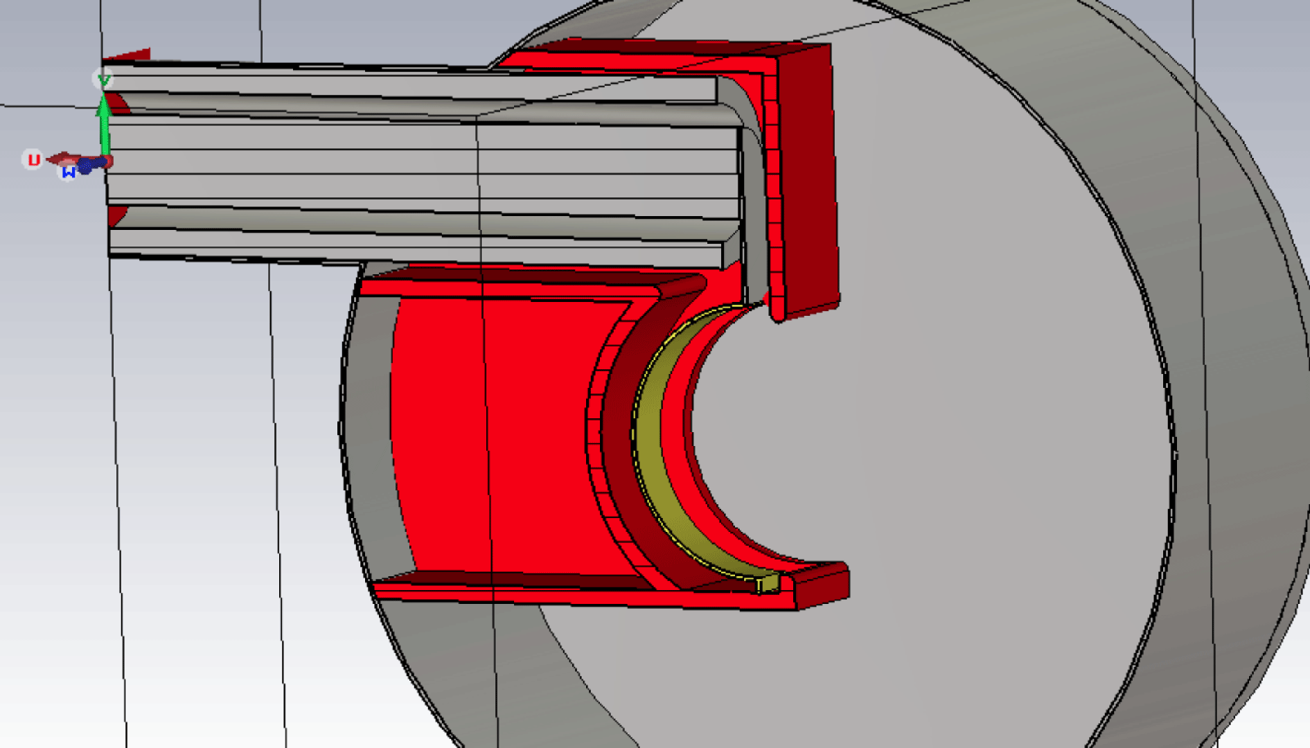
-field and plasma density. The antenna can be fed by transmission lines that are connected to the ASDEX generators, with an ample amount of power available. For the first operations, however, a low power (up to 1 kW) generator will be used, with a frequency range (0.1–100 MHz). The most optimal operating frequency for the ICRF antenna had to be found in view of the RF sheath studies, thus by preference covering a sufficiently wide density range, with distinct regions for slow and fast wave propagation and the crossing of the lower hybrid resonance (LHR) layer. Figure 1 shows a schematic design of the antenna, more technical details about IShTAR can be found in Crombé et al. (Reference Crombé2015), D’Inca et al. (Reference D’Inca2015), Louche et al. (Reference Louche2015) and fall outside the scope of this paper.
Schematic picture of the design of the antenna in IShTAR.

3 Solutions of the cold plasma dispersion relation in the edge region of a tokamak
3.1 Coupled and decoupled solutions
In a homogeneous, magnetised plasma, the wave equation reads (Stix Reference Stix1992; Brambilla Reference Brambilla1998)
 $$\begin{eqnarray}\boldsymbol{k}\times (\boldsymbol{k}\times \boldsymbol{E})+k_{0}^{2}\unicode[STIX]{x1D646}\boldsymbol{\cdot }\boldsymbol{E}=0,\end{eqnarray}$$
where
 $\boldsymbol{k}$
is the wave vector,
 $\boldsymbol{E}$
the electric field associated with the wave,
 ${\it\omega}$
the angular frequency of the wave in vacuum,
 $k_{0}={\it\omega}/c$
the vacuum wavelength with
 $c$
the speed of light and
 $\unicode[STIX]{x1D646}$
the plasma dielectric tensor.
In the cold approximation and for a magnetic field
 $B_{0}$
in the
 $z$
-direction, the plasma dielectric tensor can be written as:
 $$\begin{eqnarray}\unicode[STIX]{x1D646}=\left(\begin{array}{@{}ccc@{}}S & -\text{i}D & 0\\ \text{i}D & S & 0\\ 0 & 0 & P\end{array}\right),\end{eqnarray}$$
using the Stix formulation; the elements
 $S$
,
 $D$
and
 $P$
are given in Stix (Reference Stix1992). The wave equation (3.1) can be rewritten as:
 $$\begin{eqnarray}\left(\begin{array}{@{}ccc@{}}k_{0}^{2}S-k_{\Vert }^{2} & -\text{i}k_{0}^{2}D & k_{\bot }k_{\Vert }\\ \text{i}k_{0}^{2}D & k_{0}^{2}S-k_{\Vert }^{2}-k_{\bot }^{2} & 0\\ k_{\bot }k_{\Vert } & 0 & k_{0}^{2}P-k_{\bot }^{2}\end{array}\right)\left(\begin{array}{@{}c@{}}E_{x}\\ E_{y}\\ E_{z}\end{array}\right)=0,\end{eqnarray}$$
where
 $k_{\Vert }$
and
 $k_{\bot }$
are respectively the parallel and perpendicular components of the wave vector with respect to
 $B_{0}$
. Equation (3.3) has non-trivial solutions if the determinant of the
 $3\times 3$
matrix is equal to zero, which leads to a fourth-order equation in
 $k_{\bot }$
:
 $$\begin{eqnarray}Ak_{\bot }^{4}+Bk_{\bot }^{2}+C=0.\end{eqnarray}$$
Here
 $A$
,
 $B$
and
 $C$
are respectively given by:
 $$\begin{eqnarray}\displaystyle & A=S, & \displaystyle\end{eqnarray}$$
 $$\begin{eqnarray}\displaystyle & B=k_{\Vert }^{2}[P+S]-k_{0}^{2}[S^{2}-D^{2}+PS] & \displaystyle\end{eqnarray}$$
and
 $$\begin{eqnarray}C=P[k_{0}^{2}[S^{2}-D^{2}]+k_{\Vert }^{4}-2k_{0}^{2}k_{\Vert }^{2}S].\end{eqnarray}$$
The full (or coupled) solutions for
 $k_{\bot }^{2}$
are:
 $$\begin{eqnarray}\displaystyle & \displaystyle k_{\bot ,1}^{2}=\frac{-B+\sqrt{(B^{2}-4AC)}}{2A} & \displaystyle\end{eqnarray}$$
 $$\begin{eqnarray}\displaystyle & \displaystyle k_{\bot ,2}^{2}=\frac{-B-\sqrt{(B^{2}-4AC)}}{2A}. & \displaystyle\end{eqnarray}$$
Due to the difference between the ion and electron mass,
 $P$
is commonly much bigger than
 $S$
and
 $D$
. Exploiting this fact for the case where
 $B^{2}\gg 4AC$
yields the commonly known roots of the decoupled roots, a fast wave (FW) and a slow wave (SW):
 $$\begin{eqnarray}\displaystyle & \displaystyle k_{\bot ,FW}^{2}=\frac{[k_{0}^{2}S-k_{\Vert }^{2}]^{2}-[k_{0}^{2}D]^{2}}{k_{0}^{2}S-k_{\Vert }^{2}}=\frac{[k_{0}^{2}R-k_{\Vert }^{2}][k_{0}^{2}L-k_{\Vert }^{2}]}{k_{0}^{2}S-k_{\Vert }^{2}} & \displaystyle\end{eqnarray}$$
 $$\begin{eqnarray}\displaystyle & \displaystyle k_{\bot ,SW}^{2}=\frac{P}{S}[k_{0}^{2}S-k_{\Vert }^{2}]. & \displaystyle\end{eqnarray}$$
Equation (3.10) is the dispersion equation root for the decoupled fast wave;
 $R$
and
 $L$
can be found in Stix (Reference Stix1992). The fast wave has a cutoff at
 $k_{0}^{2}L=k_{\Vert }^{2}$
and at
 $k_{0}^{2}R=k_{\Vert }^{2}$
, the former being typical for the high density region and the latter for the low density region. Equation (3.11) characterises the slow wave. In view of the difference in size of
 $P$
w.r.t.
 $S$
and
 $D$
it can readily be seen that the wavelength of the slow wave is significantly shorter than that of the fast wave. Furthermore, the slow wave has a cutoff at
 $P=0$
and a resonance at
 $S=0$
, the latter being known as the lower hybrid resonance (LHR). Note that the decoupled slow wave cutoff location at
 $k_{0}^{2}S=k_{\Vert }^{2}$
coincides with a resonance for the decoupled fast wave. Plotting the roots of the full dispersion equation demonstrates that this point is actually a confluence. Although extremely useful in many cases, the decoupled roots do not uniformly reflect the actual physics.
3.2 Wave behaviour for typical tokamak parameters
The cold plasma description is adequate when doing wave studies in the edge of a tokamak, where temperatures are sufficiently low (normally a few tens of eV). Hence, they are used as standard when addressing topics of wave dynamics between the last closed flux surface of the tokamak and the launchers, be it that antenna design is routinely done assuming the density is low enough to neglect the presence of the plasma altogether at the location of the antenna straps inside the antenna box. Densities vary from nearly zero at the level of the antenna launcher to
 $10^{17}{-}10^{18}~\text{m}^{-3}$
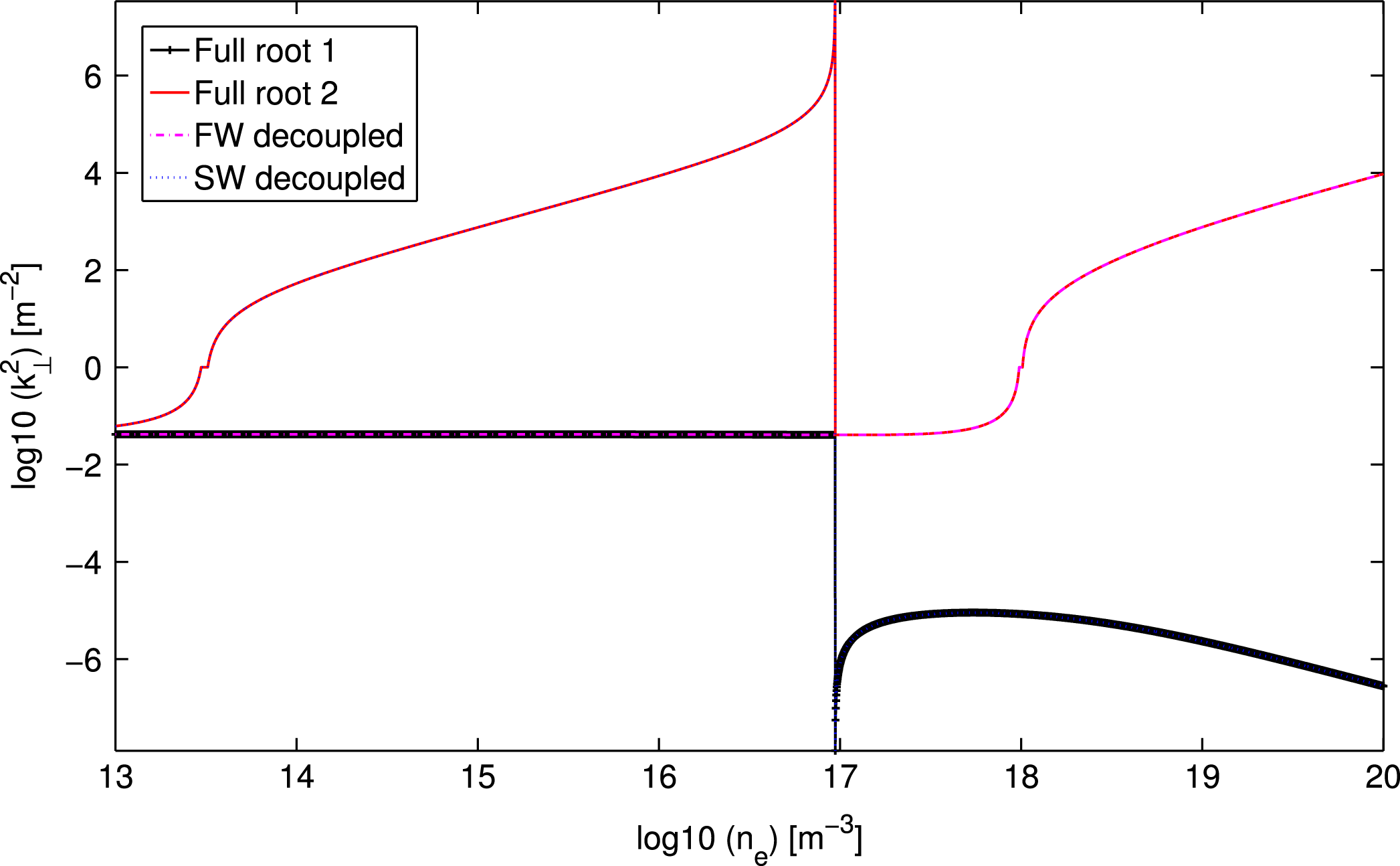
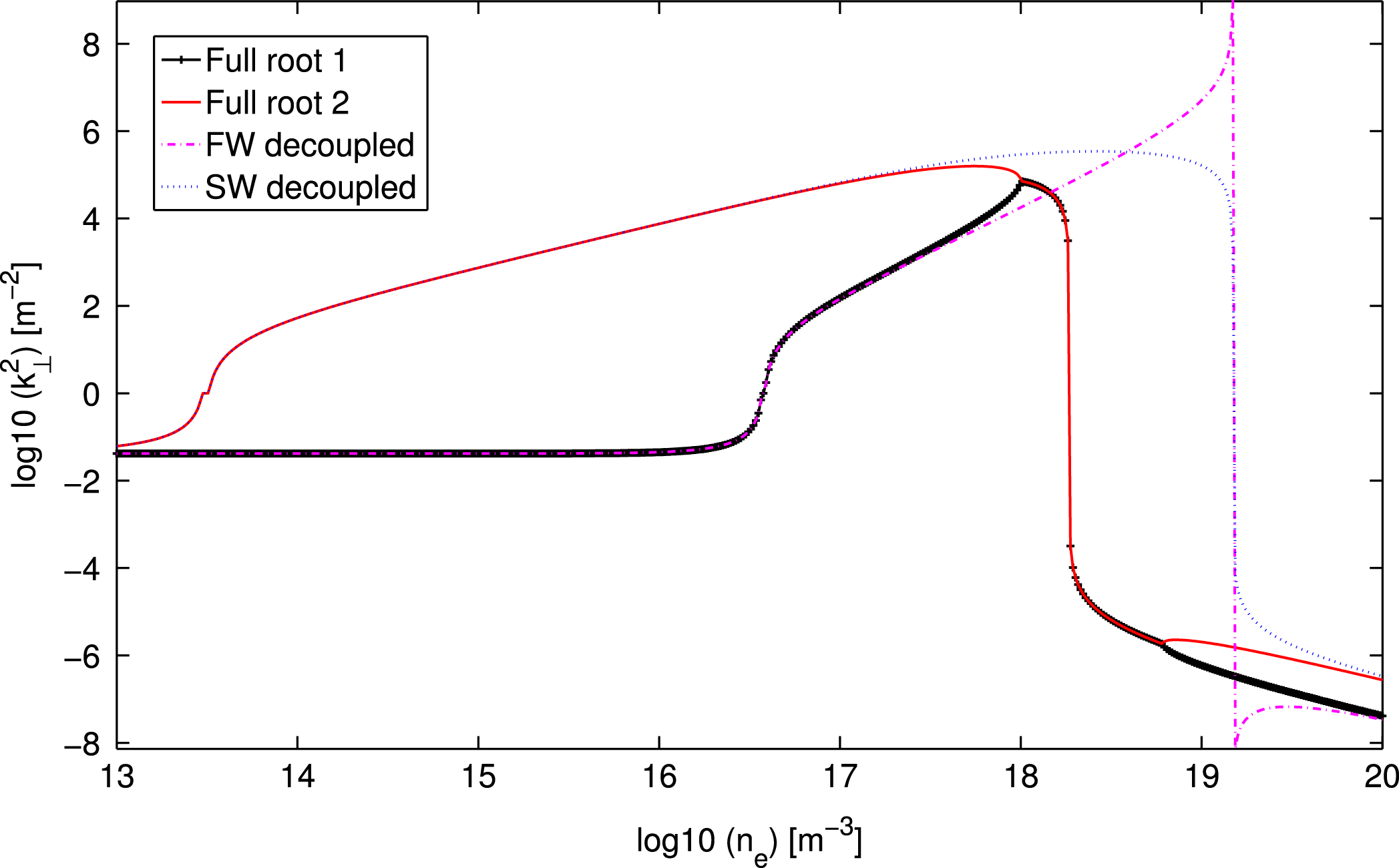
at the plasma edge. Behind the last closed flux surface, the density typically decays exponentially with a decay length of a few cm. For typical tokamak edge conditions, the lower hybrid resonance layer, the low density fast wave cutoff and the slow wave cutoff are crossed at some point going from the antenna strap towards the central plasma. Depending on the exact parameters, these cutoffs and the resonance occur inside the antenna box or in front of it. Because in antenna codes the low density region is mostly not taken into account and replaced by a vacuum layer, the reality that the plasma impacts sensitively on the wave behaviour is typically sidestepped, which potentially has severe consequences on predictions of the coupled power and which does not allow adequate description of the near-field pattern that is crucial for describing the non-resonant acceleration of particles, thought to be the origin of sputtering. Theoretical and experimental verification of how the wave–plasma cross-talk actually happens seems crucial for optimising antenna designs. At the lower hybrid resonance, one of the roots of the dispersion equation (the slow wave in the decoupled formulation) changes its behaviour from propagative (for densities just below the LHR) to evanescent (for densities just above the LHR). In figure 2 the perpendicular wave vector
 $\boldsymbol{k}_{\bot }^{2}$
is plotted as a function of the density in the range (
 $10^{13}{-}10^{20}~\text{m}^{-3}$
). The calculations were done for parameters relevant for the edge region of tokamak plasmas: a magnetic field
 $B_{0}=2.0$
T, an antenna frequency
 $f=50$
MHz, the dominant parallel wave component
 $k_{\Vert }=5~\text{m}^{-1}$
of a typical dipole spectrum, a temperature
 $T_{e}=10$
eV and for a plasma composed of 95 % of deuterium and 5 % of hydrogen. Under these conditions the LHR (i.e. where
 $k_{\bot }^{2}$
goes to infinity) is located just below
 $10^{17}~\text{m}^{-3}$
, as can be seen on the figure. The cutoffs (i.e. where
 $k_{\bot }^{2}$
goes through zero) for slow and fast wave are also visible on the plot. The cutoffs are located around density values of the order of
 $5\times 10^{13}~\text{m}^{-3}$
and
 $1\times 10^{18}~\text{m}^{-3}$
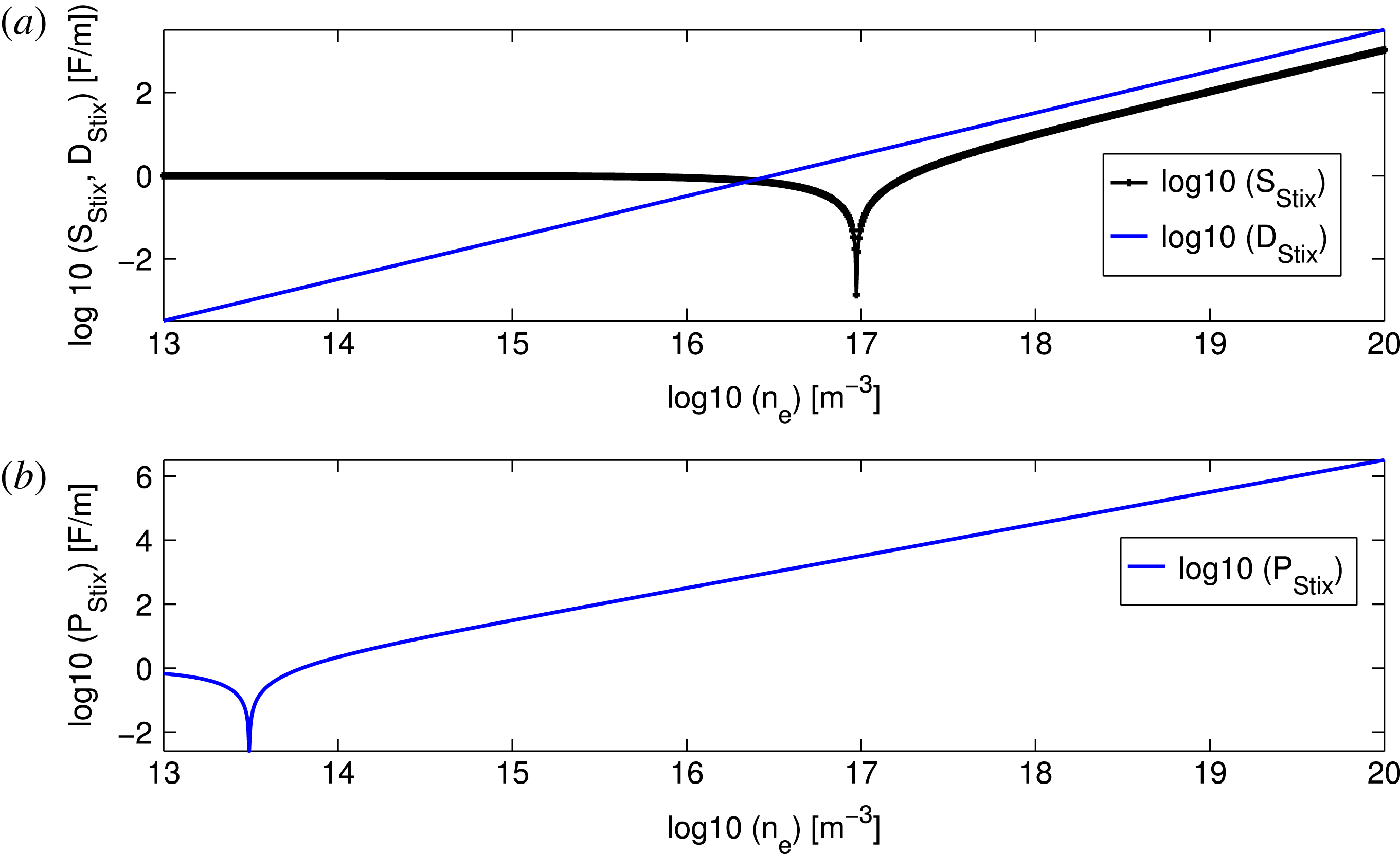
, respectively. Figure 3 provides the corresponding Stix parameters,
 $S$
,
 $D$
and
 $P$
of the dielectric tensor. The
 $P$
value (responsible for the dielectric response in the direction parallel to the magnetic field) rises quickly with density, to values that are several orders of magnitude larger than the perpendicular (
 $S$
and
 $D$
) components,
 $10^{6}$
and above, compared to
 $10^{1}$
. The underlying reason is that both the cyclotron frequency and the square of the plasma frequency scale inversely with the particle mass, which means that the electron contribution dominates that of the ions in
 $P$
and that typically
 $P\gg S,D$
on account of the very different masses of ions and electrons (recall that
 ${\it\omega}\approx O({\it\Omega}_{i})\ll |{\it\Omega}|_{e}$
). However, for low densities, and even up to the LHR layer, the
 $S$
,
 $D$
and
 $P$
, have values of order
 $1{-}10^{2}$
. This means – opposite to what is the case for typical core tokamak parameters – that the three directions are of comparable relative importance. For that reason the near-antenna field physics is very different from the core ICRF heating physics.
 $k_{\bot }^{2}$
values for full and decoupled solutions as a function of the plasma density and for typical tokamak parameters. The notation ‘log10’ denotes
 $\text{sign}(F)\log _{10}(|F|)$
when
 $|F|>1$
and 0 when
 $|F|<1$
. This notation is introduced to enable capturing of the very different length scales of the modes the cold plasma supports while allowing easy identification of regions of wave propagation and evanescence via the sign of
 $\log _{10}(k_{\bot }^{2})$
. In the low density region, both roots approach the vacuum limit,
 $k_{\bot }^{2}=k_{0}^{2}-k_{\Vert }^{2}$
, as expected, while at higher densities representative for the core, one roots is propagative (FW) and the other is deeply evanescent (SW).

Stix parameters
 $S$
,
 $D$
and
 $P$
, as a function of the plasma density, and for typical tokamak parameters.

4 Scan of the operational domain and consequences for the wave behaviour
4.1 Test bed parameters
The maximal magnetic field in IShTAR is
 $B_{0}=0.24$
T, and presently in standard operation it is limited to
 $B_{0}=0.10$
T. As the magnetic field is one of the key ingredients setting apart a dielectric medium from a magnetised plasma, this restriction is potentially severe. Moreover – at least currently (Crombé et al.
Reference Crombé2015; D’Inca et al.
Reference D’Inca2015; Louche et al.
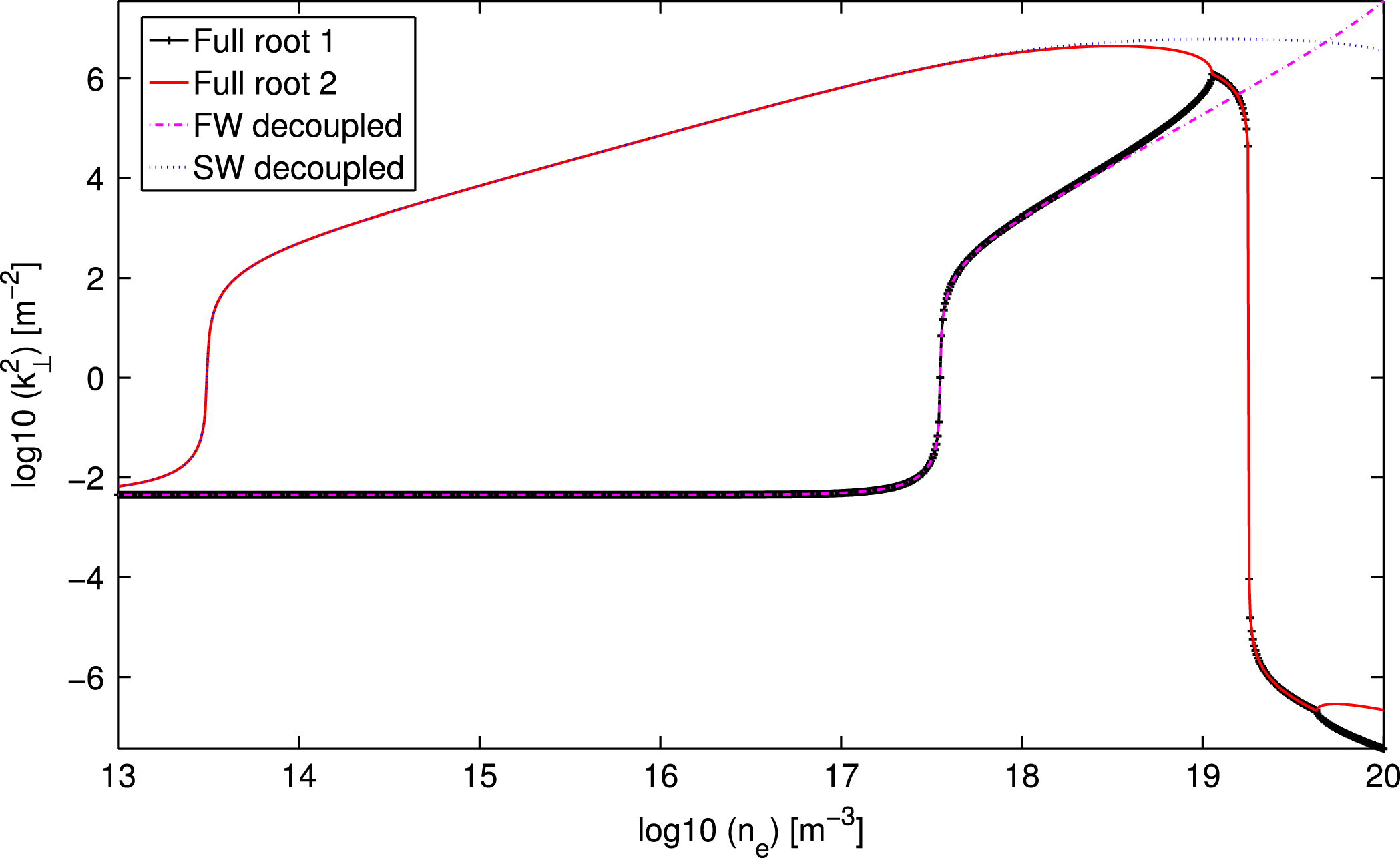
Reference Louche2015) – the densities reached in IShTAR are smaller than those in the tokamak scrape-off layer. In figures 4 and 5,
 $k_{\bot }^{2}$
is plotted for the same conditions as figure 2, but now with the magnetic field is reduced to
 $B_{0}=0.10$
T. Figure 4 shows the solutions for a (95 % D, 5 % H) plasma and
 $k_{\Vert }=15~\text{m}^{-1}$
, whereas figure 5 is for a 100 % argon plasma and
 $k_{\Vert }=5~\text{m}^{-1}$
. An important thing to note regarding the figures is that the coupled and decoupled solutions are now different around the LHR, in fact the coupled solutions (which are the more correct ones) do not show the typical signature of a LHR as for the
 $B_{0}=2.0$
T case. Furthermore, in figure 4 it can be seen that a higher
 $k_{\Vert }$
value moves the interesting region for sheath studies to density values in the range
 $10^{17}{-}10^{20}~\text{m}^{-3}$
, which is outside the present operational domain. Argon is the main gas used for the initial operation phase of IShTAR because it is easier to handle than hydrogen. Operation with other gases, such as helium and hydrogen, are foreseen for future campaigns. The wave behaviour in an argon plasma situation is plotted in figure 5. The cutoff for the second root (FW type) is now moved to lower densities, to around
 $7\times 10^{17}~\text{m}^{-3}$
instead of
 $1\times 10^{18}~\text{m}^{-3}$
for the ‘tokamak’-case. For both roots (FW and SW type) a change from propagative to evanescent behaviour occurs at the same densities interval (
 $1\times 10^{18}{-}5\times 10^{18}~\text{m}^{-3}$
). The conclusion is clear: the test bed situation is very different from the tokamak edge with respect to wave propagation. However, understanding the interaction of the two modes is crucial and should experimentally be addressed in IShTAR, because it moreover aims at studying the consequences of this wave behaviour on the plasma density, the creation of static electric fields, material sputtering and formation of hot spots. A ‘fast wave antenna’ relies on running a current through a poloidally oriented strap to excite the fast wave, but such a current equally parasitically excites the slow wave in a magnetised plasma in which the poloidal component is non-zero. This can readily be checked by evaluation of the wave equation such that for a finite magnetic field, the poloidal electric field component at the antenna forces the radial component to be finite, and the latter in turn means that the parallel component is finite. The slow wave is propagative at densities between
 $S=0$
and
 $k_{0}^{2}S=k_{\Vert }^{2}$
and carries energy away from the antenna to the LHR. In Van Eester et al. (Reference Van Eester, Crombé and Kyrytsya2013a
,Reference Van Eester, Crombé and Kyrytsya
b
) the interested reader can find examples of the slow wave exponentially decaying or adding a short wavelength propagation signature to the electric field structure close to the launcher. Such behaviour is at odds with the usual assumption that a fast wave antenna merely excites fast waves which need to tunnel through the evanescence layer to reach the
 $k_{0}^{2}R=k_{\Vert }^{2}$
cutoff and that the slow wave plays no role in the process.
 $k_{\bot }^{2}$
values for full and decoupled solutions as a function of the plasma density for similar parameters as in figure 2, but with a lower magnetic field value
 $B_{0}=0.1$
T and for
 $k_{\Vert }=15~\text{m}^{-1}$
.

 $k_{\bot }^{2}$
values for full and decoupled solutions as a function of the plasma density for similar parameters as in figure 4, but for a pure argon plasma (with partial ionisation
 $8^{+}$
).

4.2 Exploring the parameter domain
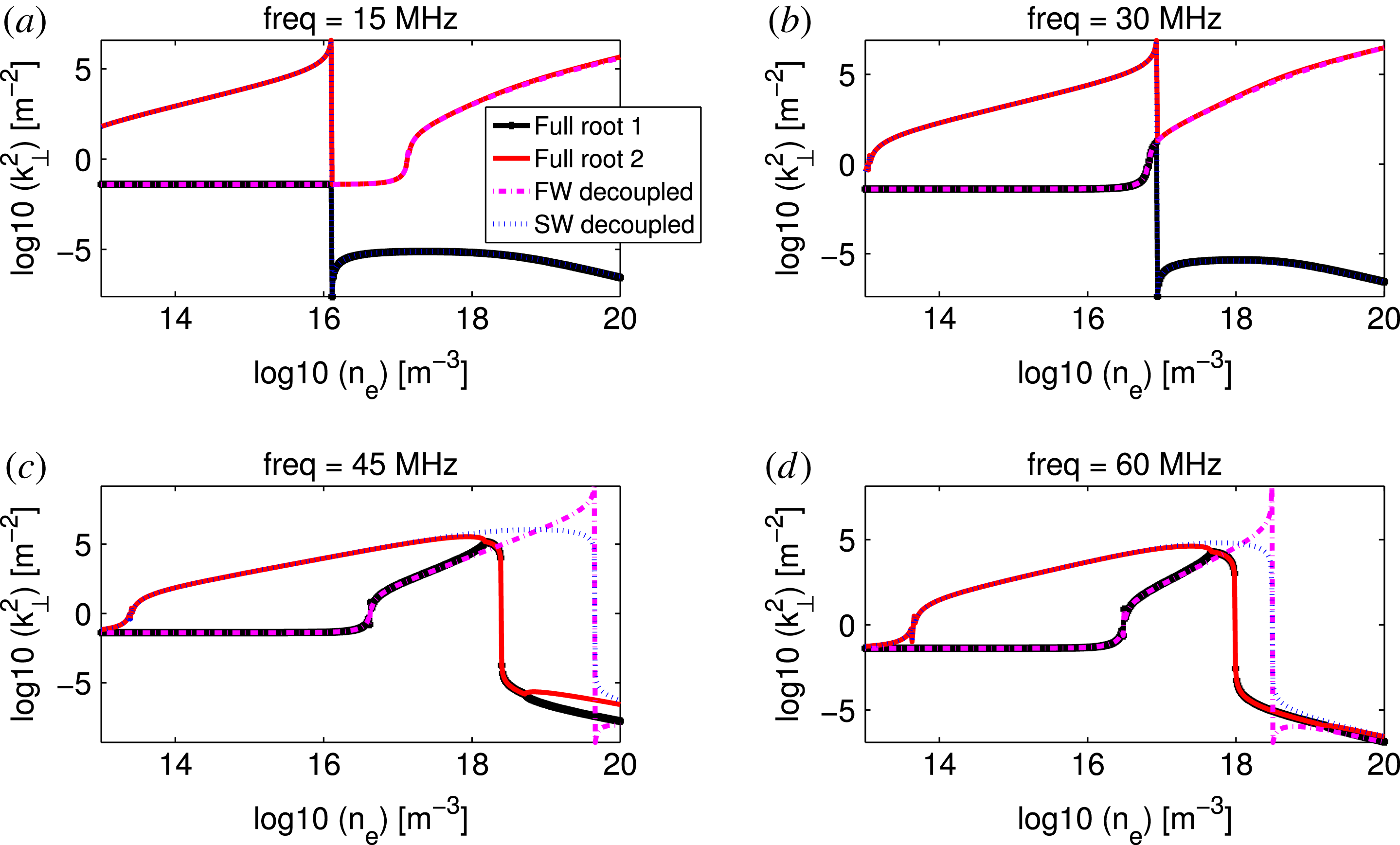
The reason for the difference in behaviour with respect to the tokamak case can be understood by scanning the frequency domain. In figure 6 four different operating frequencies are plotted in the range (15–60 MHz). For low frequencies (e.g. the 15 MHz case) the wave behaviour is similar to the standard tokamak scenario, with a slow and fast wave cutoff at clearly distinct densities and a typical LHR that only affects the SW, since the FW is still evanescent for that density. However for increasing frequencies (e.g. the 30 MHz case), the SW and FW cutoffs move closer to each other, and the FW becomes propagative at densities below the LHR (e.g. the 45 MHz case). At that moment (and this continues for even higher frequencies, e.g. the 60 MHz case) the effect of the resonance is visible on both waves as a sudden change from propagative to evanescent behaviour. Therefore, for studying the interaction characteristics of the RF waves and the plasma in the region between the antenna and the LCFS in a tokamak, adopting frequencies of
 ${\sim}$
10 MHz must be envisaged, with the densities and magnetic fields that are obtainable in IShTAR. In addition, a lower operating frequency pushes the LHR towards lower densities – level
 $10^{16}~\text{m}^{-3}$
for 15 MHz instead of
 $10^{18}~\text{m}^{-3}$
for the 50 MHz example – which are easier to reach in the test bed.
 $k_{\bot }^{2}$
values for full and decoupled solutions as a function of the plasma density for similar parameters as in figure 5, but different frequencies: 15, 30, 45 and 60 MHz.

Since the Stix parameters also depend on the magnetic field, the role of the
 $B_{0}$
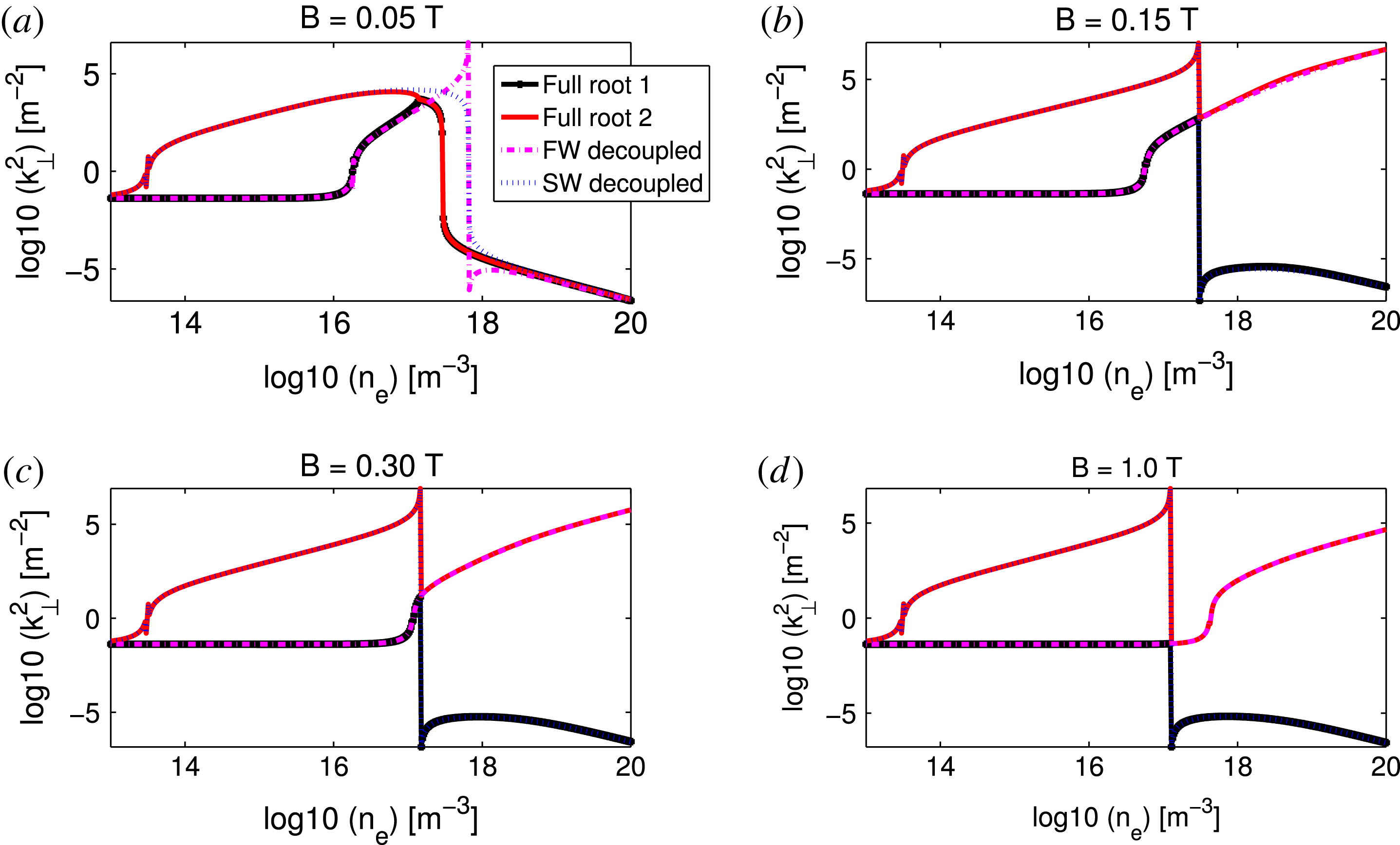
value was investigated, and is illustrated in figure 7 for various amplitudes:
 $B_{0}=0.05$
T,
 $B_{0}=0.15$
T,
 $B_{0}=0.30$
T and
 $B_{0}=1.0$
T. The calculations were performed for a fixed frequency of 50 MHz. An increasing magnetic field moves the fast wave cutoff towards higher densities. At
 $B_{0}=0.30$
T, the fast wave starts propagating only at around the LHR, and above that value the more standardly known separation between fast and slow waves is recovered. Presently IShTAR experiments are performed at
 $B_{0}=0.10$
T, as this creates the most homogeneous magnetic field configuration between the plasma source and the main vessel (Crombé et al.
Reference Crombé2015; D’Inca et al.
Reference D’Inca2015; Louche et al.
Reference Louche2015). However, if the large magnetic field coils would be operated at maximal current of 8 kA instead of 2.4 kA, a field of
 $B_{0}=0.24$
T would be achievable, which could allow us to drive the antenna at higher frequencies while keeping the standard SW and FW behaviour similar to the tokamak conditions. A drawback of the higher frequency is that higher densities – outside the range of what presently can be reached in IShTAR – are needed to cross the LHR. The advantage would be that ASDEX generators can be used, which are available and can deliver high power to the antenna. At the moment only a low power (up to 1 kW) generator is available for the 10 MHz range of frequencies. As the usual collisionless damping mechanisms active in the core of tokamaks are absent, the waves inside IShTAR are poorly damped. Although standing wave patterns that will sensitively depend on the density profiles are bound to be set-up (making the analysis non-straightforward) these modest power levels are thought to be sufficient to initiate the study.
 $k_{\bot }^{2}$
values for full and decoupled solutions as a function of the plasma density for similar parameters as in figure 5, but different values of the
 $B$
-fields: 0.05, 0.15, 0.30 and 1.0 T.

Different gases can be used in the test facility. A dispersion equation study reveals that the choice of the working gas does not significantly modify the location of the relevant resonance and cutoffs. Hence, from the RF point of view, whatever gas is most easy to handle is suitable for the study.
5 Conclusions
It has been shown that the full and decoupled roots of the cold plasma dispersion relation can be quite different at a resonance layer. In that case, the standard technique of decoupling the solutions into a slow and fast wavelength branch is not valid. Furthermore, the traditional picture of a clearly distinct density region for fast and slow wave propagation and evanescence is not a general feature. It strongly depends on the values of frequencies and magnetic field that are used. As a practical example, the dispersion equation roots were discussed for the IShTAR test bed on which it is intended to study near-field physics and plasma–wave interaction with a focus on sheaths and RF-induced density depletion. Although operating at usual tokamak parameters is impossible in IShTAR, a parameter range that allows for a suitable imitation, and in which all ingredients (lower hybrid resonance, fast and slow wave cutoffs) thought to be important occur for densities and magnetic field values, has been found.
Acknowledgements
This work has been carried out within the framework of the EUROfusion Consortium and has received funding from the Euratom research and training programme 2014–2018 under grant agreement no. 633053. The views and opinions expressed herein do not necessarily reflect those of the European Commission. The views and opinions expressed herein do not necessarily reflect those of the European Commission. The work received support from the Research Foundation Flanders (G0B3115N).