1 Introduction
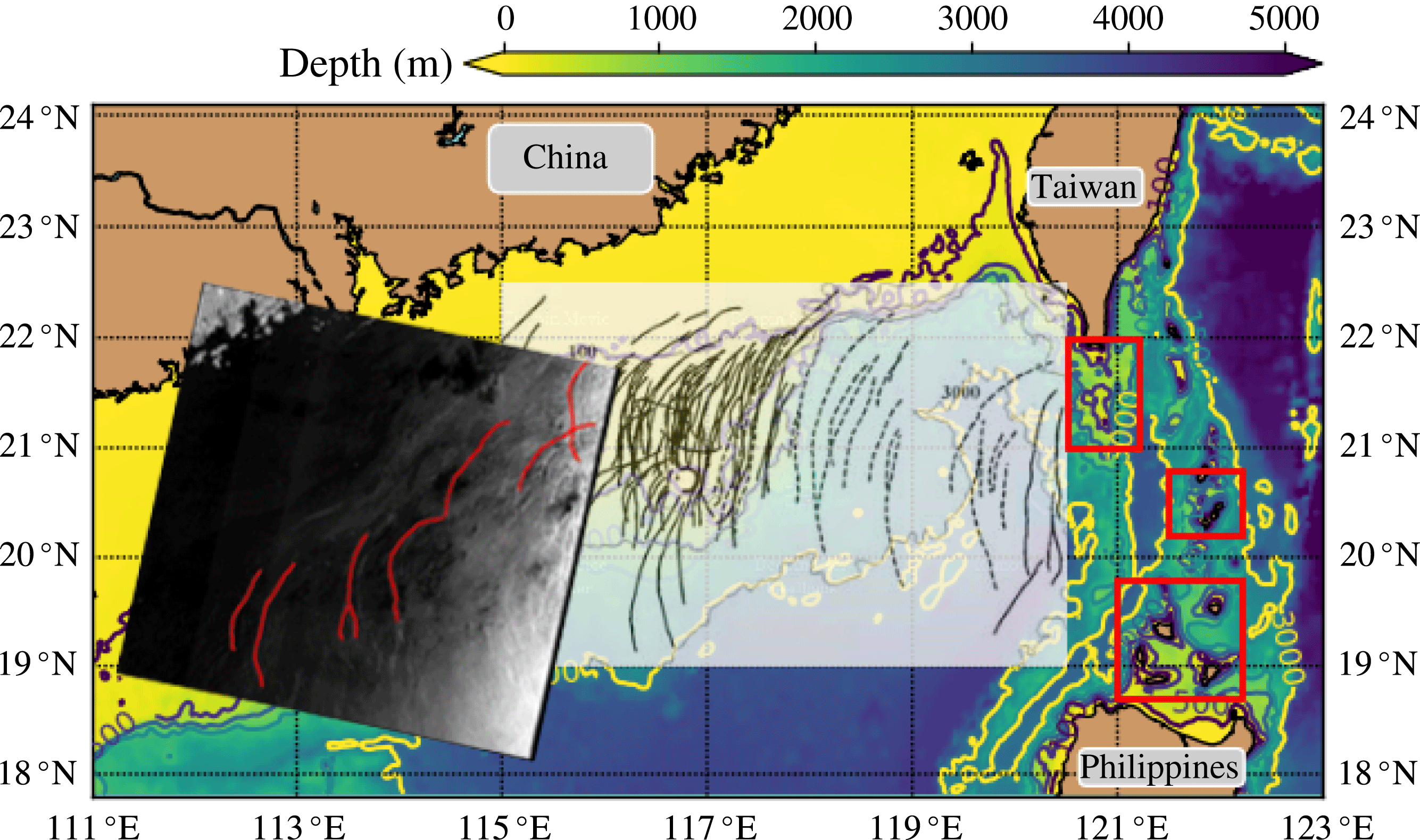
Oceanic internal solitary waves (ISWs hereinafter) are often characterised by strong nonlinearity, and have been heavily studied over the past several decades. These waves are important owing to their roles in transporting sediments, boosting biological productivity and posing potential hazards on submersibles and offshore marine structures, see for instance Osborne, Burch & Scarlet (Reference Osborne, Burch and Scarlet1978), Bogucki, Dickey & Redekopp (Reference Bogucki, Dickey and Redekopp1997), Wang, Dai & Chen (Reference Wang, Dai and Chen2007) amongst many others. These nonlinear internal waves are generated mainly through the interaction between tidal currents and abrupt topographic features, see the review by Helfrich & Melville (Reference Helfrich and Melville2006) and more recently Alford et al. (Reference Alford, MacKinnon, Nash, Simmons, Pickering, Klymak, Pinkel, Sun, Rainville, Musgrave, Beitzel, Fu and Lu2011) for instance. Due to the complicated bathymetry, there could be more than one potential generation site in a coastal ocean; for instance, in the South China Sea (SCS), three parts of the Luzon Strait are indicated as the major generation sites, see Jan, Lien & Ting (Reference Jan, Lien and Ting2008), Alford et al. (Reference Alford, MacKinnon, Nash, Simmons, Pickering, Klymak, Pinkel, Sun, Rainville, Musgrave, Beitzel, Fu and Lu2011), Guo & Chen (Reference Guo and Chen2014), also see figure 1. After radiating from their generation sites, these waves experience nonlinear steepening to evolve into ISWs, some of which have been recorded by in situ measurements and compared to the analytical Korteweg–de Vries (KdV) theory, see Yang et al. (Reference Yang, Tang, Chang, Liu, Hsu and Ramp2004), Klymak et al. (Reference Klymak, Pinkel, Liu, Liu and David2006) amongst many others. Note that although the KdV equation may not be adequate for describing such large-amplitude waves as recorded in the above literature, for example see the comparisons between the KdV theory and a fully nonlinear model in Lamb & Yan (Reference Lamb and Yan1996), the observed waveform and phase speed of ISWs are reasonably consistent with it. Then ISWs propagate onto the continental slope shelf to begin the shoaling process, see Duda et al. (Reference Duda, Lynch, Irish, Beardsley, Ramp, Chiu, Tang and Yang2004), Ramp et al. (Reference Ramp, Tang, Duda, Lynch, Liu, Chiu, Bahr, Kim and Yang2004), Fu et al. (Reference Fu, Wang, Laurent, Simmons and Wang2012) and the review by Guo & Chen (Reference Guo and Chen2014) for more details. Further, due to the variable oceanic background, ISWs can undergo refraction and reflection, see Liu & Hsu (Reference Liu and Hsu2004), Ramp et al. (Reference Ramp, Tang, Duda, Lynch, Liu, Chiu, Bahr, Kim and Yang2004), Cai & Xie (Reference Cai and Xie2010). These factors jointly create the possibility that oblique interactions between two or more ISWs can occur, see figure 1.
The bathymetry of the South China Sea. Three red rectangles indicate the potential generation sites, see Guo & Chen (Reference Guo and Chen2014). The transparent inset, adopted from Zhao et al. (Reference Zhao, Klemas, Zheng and Yan2004), shows the existence of the multi-wave ISW packets (solid line) and single-wave ISW packets (dashed line), which is a collection of the satellite images acquired from 1995 to 2001. An Envisat-1 Advanced SAR satellite image taken on 02:20 UTC, 31-07-2010 is also imposed, where some wave crestlines are accentuated in red lines.
In practice, in situ data are often limited by the spatial coverage, which inherently makes it difficult to capture a complete process of oblique wave interactions. In contrast, satellite radar images can cover a large area up to the scale of several hundred kilometres within one snapshot, although they are restricted by the long time sampling interval of a single sensor. In the world’s ocean, a large number of wave interactions have been recorded using satellite synthetic aperture radar (SAR) images; for instance, in the South China Sea, see Hsu, Liu & Liu (Reference Hsu, Liu and Liu2000), Chen et al. (Reference Chen, Liu, Wang and Hsu2011); in the Mid-Atlantic Bight, see Xue et al. (Reference Xue, Graber, Romeiser and Lund2014); off the cost of south-west Africa, see Zheng et al. (Reference Zheng, Klemas, Yan, Wang and Kagleder1997); complete coverage is available in the internal wave atlas, see Jackson (Reference Jackson2004). Satellite images themselves are usually unable to provide the interior wave structure and the associated motions directly, but nevertheless, Wang & Pawlowicz (Reference Wang and Pawlowicz2012) investigated four cases of internal wave interactions in the Strait of Georgia using sequential photogrammetrical images acquired from an aircraft, and importantly, supplementary simultaneous collections of water column properties measured by a surface vessel.
Theoretical exploration of oblique solitary wave–wave interactions in the water wave context began several decades ago with the pioneering work by Miles (Reference Miles1977a ,Reference Miles b ), who investigated the interaction between two crossing small-amplitude shallow water surface solitary waves, each governed by the KdV equation. It was found that depending on the amplitudes and angles, a Mach stem (that is a resonant phase shift) can arise in the interaction zone. After this work, laboratory experiments by Melville (Reference Melville1980), numerical simulations by Funakoshi (Reference Funakoshi1980), Tanaka (Reference Tanaka1993) and further theoretical analyses by Johnson (Reference Johnson1982) confirmed this theory, albeit only strictly valid for small-amplitude waves. More recently, Kodama (Reference Kodama2010), Yeh, Li & Kodama (Reference Yeh, Li and Kodama2010) modified the Miles theory and extended its applicability to small but finite incident angles. In this limit the Kadomtsev–Petviashvili (KP) equation has emerged as the canonical model for the description of oblique wave–wave interactions. It is a two-dimensional (2-D) version of the well-known KdV equation, albeit formally only for weak transverse effects. It was first derived by Kadomtsev & Petviashvili (Reference Kadomtsev and Petviashvili1970), and then by Grimshaw (Reference Grimshaw1981) for internal waves. Most subsequent work on oblique wave–wave interactions has focussed on the KP equation, see Kodama (Reference Kodama2010), Yeh et al. (Reference Yeh, Li and Kodama2010), Li, Yeh & Kodama (Reference Li, Yeh and Kodama2011), Kodama & Yeh (Reference Kodama and Yeh2016) for a water wave context, and Chen et al. (Reference Chen, Liu, Wang and Hsu2011), Xue et al. (Reference Xue, Graber, Romeiser and Lund2014) for internal waves. In particular Kodama, Chakravarty and colleagues developed a complete description of all two-soliton interactions within the KP context, see Chakravarty & Kodama (Reference Chakravarty and Kodama2008, Reference Chakravarty and Kodama2009, Reference Chakravarty and Kodama2013) for instance. In the internal wave context Chen et al. (Reference Chen, Liu, Wang and Hsu2011), Wang & Pawlowicz (Reference Wang and Pawlowicz2012), Xue et al. (Reference Xue, Graber, Romeiser and Lund2014) reported different internal wave–wave interaction patterns in different locations, and based their analyses largely on Miles (Reference Miles1977a ,Reference Miles b ). More recently, using a realistic oceanic background, Shimizu & Nakayama (Reference Shimizu and Nakayama2017) investigated the combined effects of variable topography and Earth’s rotation on the oblique internal solitary-like wave–wave interaction in the Andaman Sea based on the results of numerical model and the aforementioned modified Miles theory by Kodama (Reference Kodama2010), Yeh et al. (Reference Yeh, Li and Kodama2010).
Much of the previous work was for the KP equation with constant coefficients, corresponding to waves in a horizontally uniform background. Here we need a KP equation to model waves in a non-uniform medium, and so we use the form derived by Grimshaw (Reference Grimshaw1981) for internal waves on a background current with variable topography. Later Pierini (Reference Pierini1989), Cai & Xie (Reference Cai and Xie2010) invoked a similar KP model to simulate internal solitary waves in the ocean, and more recently, Yuan et al. (Reference Yuan, Grimshaw, Johnson and Chen2018b ) further developed a variable-coefficient KP (vKP) equation to study a two-dimensional topographic effect (a canyon and a submarine plateau) on the propagation of internal solitary waves, where good agreement was found between the vKP theory and a fully nonlinear non-hydrostatic general circulation model. Nonetheless, we caution that like the KdV equation for internal waves, this KP model is restricted to a single vertical mode and energy transfer between modes is explicitly excluded. In the ocean, energy transfer between mode-1 and mode-2 ISWs has indeed been observed and investigated, see Deepwell et al. (Reference Deepwell, Stastna, Carr and Davies2017), Xie et al. (Reference Xie, Li, Scully and Boicourt2017), Yuan, Grimshaw & Johnson (Reference Yuan, Grimshaw and Johnson2018a ), but usually the energy conversion is quite small, and hence is neglected here.
The vKP equation selected as our model is briefly described in § 2, followed by an introduction to a new method used to construct the KP soliton solution according to the given wave pattern. In § 2, we also present the expression of the initial V-shape waves, along with the boundary conditions implemented to solve the vKP equation. From the most commonly observed wave–wave interaction patterns, three combinations of the amplitude and angle are selected. Further, because the along-crest width can be very large in the realistic ocean, the evolution scenarios are divided into two types; one is an initial V-shape wave filling the whole transverse calculation domain, while the other one is truncated and so only occupies a portion of the domain. The model set-up and results can be found in § 3. Finally, we conclude in § 4.
2 Formulation
2.1 The variable-coefficient Kadomtsev–Petviashvili equation
In a non-rotating fluid, taking the varying background environment into consideration, the vKP equation describing the wave amplitude
 $A(x,y,t)$
can be expressed as in Grimshaw (Reference Grimshaw1981),
 $$\begin{eqnarray}\displaystyle \left[A_{t}+cA_{x}+\frac{cQ_{x}}{2Q}A+\unicode[STIX]{x1D6FC}AA_{x}+\unicode[STIX]{x1D6FD}A_{xxx}\right]_{x}+\frac{\unicode[STIX]{x1D6FE}}{2}A_{yy}=0, & & \displaystyle\end{eqnarray}$$
where
 $x,y,t$
are the horizontal spatial and temporal variables and here the subscripts denote derivatives. The linear phase speed
 $c(x,y)$
, the linear magnification factor
 $Q(x,y)$
, the nonlinear coefficient
 $\unicode[STIX]{x1D6FC}(x,y)$
and the dispersion coefficient
 $\unicode[STIX]{x1D6FD}(x,y)$
(in the
 $x$
direction),
 $\unicode[STIX]{x1D6FE}(x,y)$
can all be determined from the modal problem in the vertical direction
 $z$
,
 $$\begin{eqnarray}\displaystyle & \displaystyle \{\unicode[STIX]{x1D70C}_{0}(c-u_{0})^{2}\unicode[STIX]{x1D719}_{z}\}_{z}+\unicode[STIX]{x1D70C}_{0}N^{2}\unicode[STIX]{x1D719}=0,\quad \text{for }-h<z<0, & \displaystyle\end{eqnarray}$$
 $$\begin{eqnarray}\displaystyle & \displaystyle \unicode[STIX]{x1D719}=0\quad \text{at }z=0,-h. & \displaystyle\end{eqnarray}$$
The water depth
 $h(x,y)$
, the background stratification
 $\unicode[STIX]{x1D70C}_{0}(z;x,y)$
and background current shear
 $u_{0}(z;x,y)$
in the
 $x$
direction can vary in the horizontal directions. The stratification is usually measured by the buoyancy frequency
 $N$
, defined by
 $\unicode[STIX]{x1D70C}_{0}N^{2}=-g\unicode[STIX]{x2202}_{z}\unicode[STIX]{x1D70C}_{0}$
. Note that this modal problem in general determines an infinite number of regular modes
 $\unicode[STIX]{x1D719}_{n},n=1,2,3,\ldots$
with corresponding linear phase speeds
 $c_{n}$
, among which, usually mode-1 (
 $n=1$
) and mode-2 (
 $n=2$
) ISWs are the main interest in the ocean. Here we only consider the mode-1 waves, although observations of mode-2 waves have been reported, see Liu et al. (Reference Liu, Su, Hsu, Kuo and Ho2013), Xie et al. (Reference Xie, Li, Scully and Boicourt2017) amongst many others. Then we have, as in the well-known KdV equation,
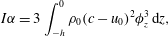 $$\begin{eqnarray}\displaystyle & \displaystyle I\unicode[STIX]{x1D6FC}=3\int _{-h}^{0}\unicode[STIX]{x1D70C}_{0}(c-u_{0})^{2}\unicode[STIX]{x1D719}_{z}^{3}\,\text{d}z, & \displaystyle\end{eqnarray}$$
 $$\begin{eqnarray}\displaystyle & \displaystyle I\unicode[STIX]{x1D6FD}=\int _{-h}^{0}\unicode[STIX]{x1D70C}_{0}(c-u_{0})^{2}\unicode[STIX]{x1D719}^{2}\,\text{d}z, & \displaystyle\end{eqnarray}$$
 $$\begin{eqnarray}\displaystyle & \displaystyle I\unicode[STIX]{x1D6FE}=2\int _{-h}^{0}\unicode[STIX]{x1D70C}_{0}(c-u_{0})^{2}\unicode[STIX]{x1D719}_{z}^{2}\,\text{d}z, & \displaystyle\end{eqnarray}$$
 $$\begin{eqnarray}\displaystyle I=2\int _{-h}^{0}\unicode[STIX]{x1D70C}_{0}(c-u_{0})\unicode[STIX]{x1D719}_{z}^{2}\,\text{d}z,\quad Q=c^{2}I. & & \displaystyle\end{eqnarray}$$
In this paper we assume that the stratification is uniform in the horizontal directions,
 $\unicode[STIX]{x1D70C}_{0}=\unicode[STIX]{x1D70C}_{0}(z)$
, and the background shear is absent,
 $u_{0}\equiv 0$
, which further leads to
 $\unicode[STIX]{x1D6FE}=c$
. In order to facilitate the dynamical analyses and numerical simulations, we make a transformation,
 $$\begin{eqnarray}\displaystyle U=Q^{1/2}A,\quad X=\int _{x_{0}}^{x}\frac{\text{d}x}{c}-t,\quad T=\int _{x_{0}}^{x}\frac{\text{d}x}{c}, & & \displaystyle\end{eqnarray}$$
where
 $x_{0}$
indicates the initial location in the
 $x$
direction. Then the asymptotically equivalent form is achieved, see Yuan et al. (Reference Yuan, Grimshaw, Johnson and Chen2018b
) for more details where, from the viewpoint of practical application, the connection with the variables in physical space is described,
 $$\begin{eqnarray}\displaystyle [U_{\unicode[STIX]{x1D70D}}+\unicode[STIX]{x1D707}UU_{X}+U_{XXX}]_{X}+\unicode[STIX]{x1D718}U_{yy}=0, & & \displaystyle\end{eqnarray}$$
 $$\begin{eqnarray}\displaystyle \unicode[STIX]{x1D70D}=\int _{0}^{T}\unicode[STIX]{x1D706}(T^{\prime })\,\text{d}T^{\prime },\quad \unicode[STIX]{x1D707}(y,\unicode[STIX]{x1D70D})=\frac{\unicode[STIX]{x1D6FC}c^{2}}{\unicode[STIX]{x1D6FD}Q^{1/2}},\quad \unicode[STIX]{x1D718}(y,\unicode[STIX]{x1D70D})=\frac{\unicode[STIX]{x1D6FE}c^{4}}{2\unicode[STIX]{x1D6FD}}. & & \displaystyle\end{eqnarray}$$
Equation (2.9) has two conservation laws,
 $$\begin{eqnarray}\displaystyle & \displaystyle \int _{-\infty }^{+\infty }U\,\text{d}X=[V]_{-\infty }^{+\infty }=0,\quad V=-\int _{X}^{+\infty }U(X^{\prime },y,\unicode[STIX]{x1D70D})\,\text{d}X^{\prime }, & \displaystyle\end{eqnarray}$$
 $$\begin{eqnarray}\displaystyle & \displaystyle \frac{\unicode[STIX]{x2202}}{\unicode[STIX]{x2202}\unicode[STIX]{x1D70D}}\int _{-\infty }^{+\infty }\frac{U^{2}}{2}\,\text{d}X+\unicode[STIX]{x1D718}\frac{\unicode[STIX]{x2202}}{\unicode[STIX]{x2202}y}\int _{-\infty }^{+\infty }UV_{y}\,\text{d}X=0, & \displaystyle\end{eqnarray}$$
for solutions
 $U(X,y,\unicode[STIX]{x1D70D})$
localised (or periodic) in
 $X$
. They represent the conservation of mass and wave action flux respectively.
2.2 Initial condition
First we consider the case of constant topography and a horizontally uniform background so that
 $\unicode[STIX]{x1D707}=\unicode[STIX]{x1D707}_{0},\unicode[STIX]{x1D718}=\unicode[STIX]{x1D718}_{0}$
are constants in the vKP equation (2.9), namely,
 $$\begin{eqnarray}\displaystyle [U_{\unicode[STIX]{x1D70D}}+\unicode[STIX]{x1D707}_{0}UU_{X}+U_{XXX}]_{X}+\unicode[STIX]{x1D718}_{0}U_{yy}=0. & & \displaystyle\end{eqnarray}$$
It can be further transformed to the canonical form,
 $$\begin{eqnarray}\displaystyle [4\unicode[STIX]{x1D6EC}_{s}+6\unicode[STIX]{x1D6EC}\unicode[STIX]{x1D6EC}_{\unicode[STIX]{x1D709}}+\unicode[STIX]{x1D6EC}_{\unicode[STIX]{x1D709}\unicode[STIX]{x1D709}\unicode[STIX]{x1D709}}]_{\unicode[STIX]{x1D709}}+3\unicode[STIX]{x1D6EC}_{YY}=0, & & \displaystyle\end{eqnarray}$$
 $$\begin{eqnarray}\displaystyle \unicode[STIX]{x1D70D}=Rs,\quad X=L\unicode[STIX]{x1D709},\quad y=MY,\quad U=P\unicode[STIX]{x1D6EC}, & & \displaystyle\end{eqnarray}$$
 $$\begin{eqnarray}\displaystyle \text{where }R=\frac{L^{3}}{4},\quad L^{2}=M^{2}=\frac{3}{\unicode[STIX]{x1D718}_{0}},\quad P=\frac{2\unicode[STIX]{x1D718}_{0}}{\unicode[STIX]{x1D707}_{0}}. & & \displaystyle\end{eqnarray}$$
From the work of Chakravarty & Kodama (Reference Chakravarty and Kodama2008, Reference Chakravarty and Kodama2009, Reference Chakravarty and Kodama2013), the KP equation (2.14) admits multi-soliton solutions which feature an arbitrary number of asymptotic line solitons in the far field and a complex wave structure formed by the interactions between intermediate solitons in the near field. One of the advantages of these solutions is they can be constructed through measuring certain characteristics of the given wave pattern, including, but not limited to, the number of line solitons in the far field (
 $Y\gg 0$
and
 $Y\ll 0$
), the amplitude and slope of each line soliton. Chakravarty & Kodama (Reference Chakravarty and Kodama2013) applied this method to the construction of an observed surface wave interaction pattern and Yeh & Li (Reference Yeh and Li2014) made a realisation of a variety of these KP soliton formations in the laboratory. Now we will briefly introduce this theory, in which the solution of equation (2.14) can be represented by
 $$\begin{eqnarray}\displaystyle \unicode[STIX]{x1D6EC}(\unicode[STIX]{x1D709},Y,s)=2(\ln \unicode[STIX]{x1D70F})_{\unicode[STIX]{x1D709}\unicode[STIX]{x1D709}}, & & \displaystyle\end{eqnarray}$$
where the
 $\unicode[STIX]{x1D70F}$
-function
 $\unicode[STIX]{x1D70F}(\unicode[STIX]{x1D709},Y,s)$
is defined as the Wronskian of
 $N$
functions
 $f_{1},\ldots ,f_{N}$
, each of which satisfy the linear equations,
 $f_{Y}=f_{\unicode[STIX]{x1D709}\unicode[STIX]{x1D709}},f_{s}=-f_{\unicode[STIX]{x1D709}\unicode[STIX]{x1D709}\unicode[STIX]{x1D709}}$
and can further be expressed as a sum of exponential functions
 $$\begin{eqnarray}\displaystyle f_{n}=\mathop{\sum }_{m=1}^{M}a_{nm}\exp (\unicode[STIX]{x1D703}_{m}),\quad \unicode[STIX]{x1D703}_{m}=\unicode[STIX]{x1D70E}_{m}\unicode[STIX]{x1D709}+\unicode[STIX]{x1D70E}_{m}^{2}Y-\unicode[STIX]{x1D70E}_{m}^{3}s,\quad n=1,2,\ldots ,N. & & \displaystyle\end{eqnarray}$$
This depends on
 $M>N$
real parameters, ordered as
 $\unicode[STIX]{x1D70E}_{1}<\cdots <\unicode[STIX]{x1D70E}_{M}$
, and the constant coefficients
 $a_{nm}$
form an
 $N\times M$
matrix
 $\mathbb{A}$
, all of whose
 $N\times N$
minors must be non-negative to ensure the non-singularity of the solution (2.17). In general, this solution consists of
 $N$
line solitons for
 $Y\gg 0$
and
 $M-N$
line solitons for
 $Y\ll 0$
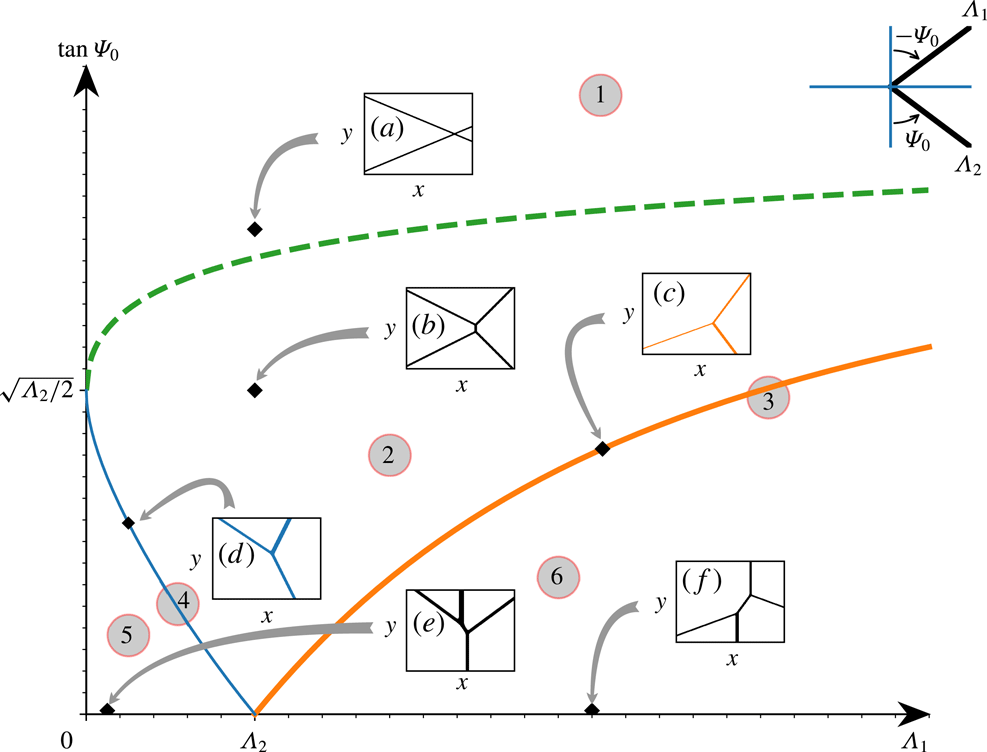
. For example, the pattern labelled by (c) in figure 2 can be interpreted as the case with
 $M=3,N=1$
.
The initial V-shape wave (2.23) is depicted in the right upper corner. In the constant-coefficient KP equation (2.14), with the amplitude of the lower branch
 $\unicode[STIX]{x1D6EC}_{2}$
fixed, the developed wave patterns which evolve corresponding to the amplitude of the upper branch
 $\unicode[STIX]{x1D6EC}_{1}$
and slope
 $\tan \unicode[STIX]{x1D6F9}_{0}$
are shown. The evolution regime can be divided into six regions, and regions 3 and 4 appear along the thick solid line (in orange) and thin solid line (in blue) respectively. The green dashed line is given by
 $\sqrt{2\unicode[STIX]{x1D6EC}_{1}}+\sqrt{2\unicode[STIX]{x1D6EC}_{2}}=2\tan \unicode[STIX]{x1D6F9}_{0}$
, the thick solid line is given by
 $\sqrt{2\unicode[STIX]{x1D6EC}_{1}}-\sqrt{2\unicode[STIX]{x1D6EC}_{2}}=2\tan \unicode[STIX]{x1D6F9}_{0}$
and the thin solid line is given by
 $\sqrt{2\unicode[STIX]{x1D6EC}_{2}}-\sqrt{2\unicode[STIX]{x1D6EC}_{1}}=2\tan \unicode[STIX]{x1D6F9}_{0}$
. A similar figure is also given in Oikawa et al. (Reference Oikawa, Tsuji, Kodama, Maruno and Isojima2010).

The solution containing only one soliton is defined by
 $M=2,N=1$
so that
 $$\begin{eqnarray}\displaystyle \unicode[STIX]{x1D70F}=\exp (\unicode[STIX]{x1D703}_{1})+a\exp (\unicode[STIX]{x1D703}_{2}), & & \displaystyle\end{eqnarray}$$
where
 $a>0$
is a free parameter and it determines the location of the soliton. Without any loss of generality, this can be recast to the following form,
 $$\begin{eqnarray}\displaystyle \unicode[STIX]{x1D70F}=1+a\exp (\unicode[STIX]{x1D703}_{2}-\unicode[STIX]{x1D703}_{1}). & & \displaystyle\end{eqnarray}$$
Then substituting (2.20) into (2.17) we have
 $$\begin{eqnarray}\displaystyle \left.\begin{array}{@{}c@{}}\displaystyle \unicode[STIX]{x1D6EC}=\unicode[STIX]{x1D6EC}_{0}\,\text{sech}^{2}\left(\frac{\unicode[STIX]{x1D6F7}+\unicode[STIX]{x1D6F7}_{0}}{2}\right),\\ \displaystyle \unicode[STIX]{x1D6EC}_{0}=\frac{k^{2}}{2}=\frac{1}{2}(\unicode[STIX]{x1D70E}_{2}-\unicode[STIX]{x1D70E}_{1})^{2},\quad \unicode[STIX]{x1D6F7}=\unicode[STIX]{x1D703}_{2}-\unicode[STIX]{x1D703}_{1}=k\unicode[STIX]{x1D709}+lY-\unicode[STIX]{x1D714}s,\quad \exp \unicode[STIX]{x1D6F7}_{0}=a,\\ \displaystyle k=\unicode[STIX]{x1D70E}_{2}-\unicode[STIX]{x1D70E}_{1},\quad l=\unicode[STIX]{x1D70E}_{2}^{2}-\unicode[STIX]{x1D70E}_{1}^{2},\quad 4\unicode[STIX]{x1D714}k=k^{4}+3l^{2},\end{array}\right\} & & \displaystyle\end{eqnarray}$$
where
 $\unicode[STIX]{x1D6EC}_{0}$
is the wave amplitude, while
 $\unicode[STIX]{x1D6F7}$
is the phase consisting of the wavenumbers
 $k,l$
in the
 $\unicode[STIX]{x1D709},Y$
directions and the frequency
 $\unicode[STIX]{x1D714}$
. There is a phase shift
 $\unicode[STIX]{x1D6F7}_{0}$
determined by the free parameter
 $a>0$
and the choice
 $a=1$
places the wave passing through the origin
 $\unicode[STIX]{x1D709}=Y=0$
at
 $s=0$
. Equation (2.21) can be further written in physical variables,
 $$\begin{eqnarray}\displaystyle \left.\begin{array}{@{}c@{}}\displaystyle \unicode[STIX]{x1D6EC}=\unicode[STIX]{x1D6EC}_{0}\,\text{sech}^{2}\,\sqrt{\frac{\unicode[STIX]{x1D6EC}_{0}}{2}}(\unicode[STIX]{x1D709}+Y\tan \unicode[STIX]{x1D6F9}-Cs+\unicode[STIX]{x1D709}_{0}),\\ \displaystyle C=\frac{1}{2}\unicode[STIX]{x1D6EC}_{0}+\frac{3}{4}\tan ^{2}\unicode[STIX]{x1D6F9},\quad \unicode[STIX]{x1D709}_{0}=\frac{\ln a}{\sqrt{2\unicode[STIX]{x1D6EC}_{0}}},\end{array}\right\} & & \displaystyle\end{eqnarray}$$
which yields the well-known KdV solitary wave. It is clear that this solution describes an oblique solitary wave whose crest line has a slope
 $\tan \unicode[STIX]{x1D6F9}$
, where the angle
 $\unicode[STIX]{x1D6F9}$
is measured counterclockwise from the
 $Y$
-axis. This oblique solitary wave is not stationary and it propagates in the positive
 $\unicode[STIX]{x1D709}$
direction with the phase speed
 $C$
; its speed in the direction normal to the crest line is
 $C\cos \unicode[STIX]{x1D6F9}$
. Note that the soliton (2.22) is defined in the mapping space (2.15) and this translates in equation (2.13) with an amplitude
 $U=P\unicode[STIX]{x1D6EC}_{0}$
and an unchanged slope
 $\tan \unicode[STIX]{x1D6F9}$
. In practice, usually
 $P=2\unicode[STIX]{x1D718}_{0}/\unicode[STIX]{x1D707}_{0}\sim O(10^{2})$
, see figure 3 for our cases, thus the magnitude of
 $\unicode[STIX]{x1D6EC}_{0}$
is usually small.
The
 $y$
-independent bathymetry
 $h$
(a); the linear phase speed
 $c$
(b); the nonlinear coefficient
 $\unicode[STIX]{x1D707}$
(c); the dispersive coefficient
 $\unicode[STIX]{x1D718}$
(d).

Our interest here is in the
 $2$
-soliton interactions which can be constructed from (2.17), (2.18). It was shown by Chakravarty & Kodama (Reference Chakravarty and Kodama2008, Reference Chakravarty and Kodama2009, Reference Chakravarty and Kodama2013) that one distinct type arises when
 $M=3,N=1$
or 2; one when
 $M=4,N=1$
or 3 and when
 $M=4,N=2$
there are seven distinct cases that can occur. Here ‘distinct’ means they cannot be obtained from another such solution through an inversion of symmetry, such as
 $(\unicode[STIX]{x1D709},Y,s)\rightarrow (-\unicode[STIX]{x1D709},-Y,-s)$
. Taking account of this theory and the observed two-ISW interactions in the ocean, we select a V-shape wave consisting of two oblique ISWs as the initial condition for the KP equation (2.9) and (2.13), that is
 $$\begin{eqnarray}\displaystyle \left.\begin{array}{@{}c@{}}\displaystyle U(X,y,\unicode[STIX]{x1D70D}=0)=U_{1}^{0}(X,y)+U_{2}^{0}(X,y),\\ \displaystyle U_{1}^{0}=U_{1}H(y)\,\text{sech}^{2}\,\sqrt{\frac{U_{1}}{2}}(X-y\tan \unicode[STIX]{x1D6F9}_{0}),\\ \displaystyle U_{2}^{0}=U_{2}H(-y)\,\text{sech}^{2}\,\sqrt{\frac{U_{2}}{2}}(X+y\tan \unicode[STIX]{x1D6F9}_{0}),\end{array}\right\} & & \displaystyle\end{eqnarray}$$
where
 $U_{1}$
and
 $U_{2}$
are the amplitudes for the upper (
 $y>0$
) and lower (
 $y<0$
) branch respectively, and their counterparts in the mapping space (2.15) are
 $\unicode[STIX]{x1D6EC}_{1}=U_{1}/P$
and
 $\unicode[STIX]{x1D6EC}_{2}=U_{2}/P$
. Here we have assumed that each branch has the same inclination with angle
 $\mp \unicode[STIX]{x1D6F9}_{0}$
relative to the
 $y$
-axis, which is measured counterclockwise.
 $h(y)$
is the Heaviside step function, defined by
 $$\begin{eqnarray}\displaystyle H(y)=\left\{\begin{array}{@{}l@{}}1,\quad y\geqslant 0,\\ 0,\quad y<0.\end{array}\right. & & \displaystyle\end{eqnarray}$$
A similar initial condition was used by Chakravarty & Kodama (Reference Chakravarty and Kodama2009) to study the oblique interaction of surface solitary water waves. More comprehensively, Kao & Kodama (Reference Kao and Kodama2012) gave a detailed numerical description of this initial V-shape condition associated with equation (2.14), and it was found that depending on the wave amplitude and angle, the V-shape wave eventually converges (asymptotically) to some of the exact soliton solutions (2.17). The main possible outcomes of interest to our present application are schematically indicated in figure 2. Patterns (a,b) can be described by
 $M=4,N=2$
and the solutions are constructed from (2.17), (2.18), which correspond to (2143) and (3142)-type solutions respectively, as in Chakravarty & Kodama (Reference Chakravarty and Kodama2008, Reference Chakravarty and Kodama2009, Reference Chakravarty and Kodama2013). Patterns (c,d) correspond to
 $M=3,N=1$
and
 $2$
whose respective solutions are (312) and (231)-type. Patterns (e,f) are (2341)-type (
 $M=4,N=3$
) and (4123)-type solutions (
 $M=4,N=1$
). Note that the pair of patterns (c,d) can be transformed between each other using the inflection from
 $y\rightarrow -y$
, and also for patterns (e,f). Pattern (a) in figure 2 was initially investigated by Miles (Reference Miles1977a
), who found the phase shift, while patterns (c,d) are resonant interactions as Miles (Reference Miles1977b
) noted. For pattern (b), a Mach stem arises in the interaction zone. There are no corresponding exact analytical soliton solutions at the critical angle
 $\unicode[STIX]{x1D6F9}_{c}$
depicted by the green dashed line in figure 2 (see Kao & Kodama Reference Kao and Kodama2012), although Kodama, Oikawa & Tsuji (Reference Kodama, Oikawa and Tsuji2009) numerically explored this case and found that the stem length has a logarithmic increase when approaching the critical angle. In practice, the critical angle
 $\unicode[STIX]{x1D6F9}_{c}$
is related to the magnitude of
 $\unicode[STIX]{x1D6EC}_{1,2}$
, see figure 2, which are usually not large, since
 $P=2\unicode[STIX]{x1D718}_{0}/\unicode[STIX]{x1D707}_{0}\sim O(10^{2})$
. There are six such wave patterns shown in figure 2, where the boundaries are given by the relations
 $\sqrt{2\unicode[STIX]{x1D6EC}_{2}}+\sqrt{2\unicode[STIX]{x1D6EC}_{1}}=2\tan \unicode[STIX]{x1D6F9}_{0}$
(a transition from pattern (a) to (b), green dashed line),
 $\sqrt{2\unicode[STIX]{x1D6EC}_{1}}-\sqrt{2\unicode[STIX]{x1D6EC}_{2}}=2\tan \unicode[STIX]{x1D6F9}_{0}$
(a transition from pattern (b) to the limiting case (c), thick solid line) and
 $\sqrt{2\unicode[STIX]{x1D6EC}_{2}}-\sqrt{2\unicode[STIX]{x1D6EC}_{1}}=2\tan \unicode[STIX]{x1D6F9}_{0}$
(a transition from pattern (b) to the limiting case (d), thin solid line). Patterns (a–c) are more often recorded for internal waves in the ocean, see Chen et al. (Reference Chen, Liu, Wang and Hsu2011), Wang & Pawlowicz (Reference Wang and Pawlowicz2012), Xue et al. (Reference Xue, Graber, Romeiser and Lund2014), and the SAR image in our figure 1. In the subsequent sections we will consider only these three cases.
In the coastal ocean, the along-crest width of the ISWs is mostly in the range from several kilometres to several hundred kilometres, for instance see Chen et al. (Reference Chen, Liu, Wang and Hsu2011), Wang & Pawlowicz (Reference Wang and Pawlowicz2012), Xue et al. (Reference Xue, Graber, Romeiser and Lund2014). Then depending on the scale of interest, two scenarios arise; one is when the initial waves fill the whole transverse calculation domain, while the other one is when they are truncated, that is, the initial waves only occupy a central part of the region. In our context, for the latter case, the initial V-shape wave (2.23) is confined in a
 $y$
-direction envelope which equals unity in a specified region
 $|y|<y_{b}$
and tapers to zero outside that range, using an envelope
 $$\begin{eqnarray}\displaystyle \text{ENV}(y)=\frac{1}{2}\left[\tanh \left(\frac{y+y_{e}}{y_{w}}\right)-\tanh \left(\frac{y-y_{e}}{y_{w}}\right)\right]. & & \displaystyle\end{eqnarray}$$
We need
 $y_{e}\gg y_{w}$
to ensure a large value of
 $y_{b}$
.
2.3 Boundary condition
An important numerical issue is the boundary condition in the
 $y$
direction. For the case that the initial along-crest width is short relative to the calculation domain, that is with the envelope
 $\text{ENV}(y)$
(2.25) imposed on the initial wave
 $U(X,y,\unicode[STIX]{x1D70D}=0)$
(2.23), two boundary layers are added to the two
 $y$
boundaries to avoid radiated waves re-entering the calculation domain. Note that in the calculated space (see (2.9)), in the
 $X$
direction, the waves propagate with the nonlinear phase speed
 $\unicode[STIX]{x1D6FC}U/3$
which is usually very small, therefore no boundaries are needed in the
 $X$
direction considering our relatively short computation time. In contrast, for the case that the initial waves fill the whole transverse domain, we use the window-scheme method, see Schlatter, Adams & Kleiser (Reference Schlatter, Adams and Kleiser2005), to transform
 $U$
into a function
 $\unicode[STIX]{x1D702}$
which equals to
 $U$
in the interior but rapidly decays to zero near the boundaries
 $y=\pm L_{y}$
, that is essentially a decomposition of
 $U$
,
 $$\begin{eqnarray}\displaystyle U=\unicode[STIX]{x1D702}+(1-W)U\quad \text{with }\unicode[STIX]{x1D702}=WU, & & \displaystyle\end{eqnarray}$$
where
 $W(y)$
is the window function defined as
 $$\begin{eqnarray}\displaystyle W(y)=\exp \left(-a\left|\frac{y}{L_{y}}\right|^{n}\right). & & \displaystyle\end{eqnarray}$$
Here we choose two parameters,
 $n=95$
and
 $a=(1.02)^{n}\ln 10$
, analogous to those in Kao & Kodama (Reference Kao and Kodama2012). This decomposition replaces the aperiodic
 $U$
with
 $\unicode[STIX]{x1D702}$
which can, with exponential accuracy, be taken as periodic in the
 $y$
-direction. We assume that outside the boundaries
 $y=\pm L_{y}$
, the solution can be described by a form
 $U_{0}$
, that is the initial condition (2.23) but moving with its corresponding phase speed
 $C$
(2.21). When the background is horizontally uniform, i.e. equation (2.13) governs the system, then this treatment is very accurate. However when variable topography is considered, this treatment will undoubtedly induce numerical errors. In the computations here the transverse length in the
 $y$
direction is sufficiently large that the central interaction zone is not affected by the boundary values over the times of computation as demonstrated by test computations on larger domains (not shown). The transverse length being large also guarantees that the post-interaction waves have no chance to re-enter the domain to contaminate the calculations. Then through the transformation,
 $$\begin{eqnarray}\displaystyle U=\unicode[STIX]{x1D702}+(1-W)U_{0}, & & \displaystyle\end{eqnarray}$$
we recast the variable-coefficient equation (2.9) to the form,
 $$\begin{eqnarray}\displaystyle \left.\begin{array}{@{}c@{}}\displaystyle [\unicode[STIX]{x1D702}_{\unicode[STIX]{x1D70D}}+\unicode[STIX]{x1D707}\unicode[STIX]{x1D702}\unicode[STIX]{x1D702}_{X}+\unicode[STIX]{x1D702}_{XXX}]_{X}+\unicode[STIX]{x1D718}\unicode[STIX]{x1D702}_{yy}=G_{1}(X,y,\unicode[STIX]{x1D70D})+G_{2}(X,y,\unicode[STIX]{x1D70D}),\\ \displaystyle G_{1}(X,y,\unicode[STIX]{x1D70D})=-(1-W)[\unicode[STIX]{x2202}_{X}(U_{0}+\unicode[STIX]{x1D707}U_{0}\unicode[STIX]{x2202}_{X}U_{0}+\unicode[STIX]{x2202}_{X}^{3}U_{0})+\unicode[STIX]{x1D718}\unicode[STIX]{x2202}_{y}^{2}U_{0}],\\ \displaystyle \!\!\!G_{2}(X,y,\unicode[STIX]{x1D70D})=\unicode[STIX]{x1D707}(1-W)\unicode[STIX]{x2202}_{X}[WU_{0}\unicode[STIX]{x2202}_{X}U_{0}-\unicode[STIX]{x2202}_{X}(\unicode[STIX]{x1D702}U_{0})]+\unicode[STIX]{x1D718}[2(\unicode[STIX]{x2202}_{y}W)(\unicode[STIX]{x2202}_{y}U_{0})\!+\!U_{0}\unicode[STIX]{x2202}_{y}^{2}W].\end{array}\right\}\qquad & & \displaystyle\end{eqnarray}$$
Recall that we have assumed
 $U_{0}$
satisfies the vKP equation (2.9) in the boundary layers, thus
 $G_{1}=0$
and only the term
 $G_{2}$
takes effect. For the horizontally uniform background, the derivation is the same except replacing
 $\unicode[STIX]{x1D707}(y,\unicode[STIX]{x1D70D}),\unicode[STIX]{x1D718}(y,\unicode[STIX]{x1D70D})$
with constants
 $\unicode[STIX]{x1D707}_{0},\unicode[STIX]{x1D718}_{0}$
.
2.4 Numerical method
The equation we are solving can be written in the form
 $$\begin{eqnarray}\displaystyle [D_{\unicode[STIX]{x1D70D}}+\unicode[STIX]{x1D707}DD_{X}+D_{XXX}]_{X}+\unicode[STIX]{x1D718}D_{yy}=R, & & \displaystyle\end{eqnarray}$$
where
 $D(X,y,\unicode[STIX]{x1D70D})$
can be either
 $U$
in equation (2.9) or
 $\unicode[STIX]{x1D702}$
in equation (2.29) depending on the specific use and
 $\unicode[STIX]{x1D707}(y,\unicode[STIX]{x1D70D}),\unicode[STIX]{x1D718}(y,\unicode[STIX]{x1D70D})$
are defined in equation (2.10). The choice of boundary conditions determines the expression of
 $R$
. If the absorbing boundary layer scheme is implemented at the
 $y$
boundaries of the calculated domain, then
 $D=U$
and
 $R=\unicode[STIX]{x1D705}(y)D_{X}$
where
 $$\begin{eqnarray}\displaystyle \unicode[STIX]{x1D705}(y)=\frac{\unicode[STIX]{x1D705}_{0}}{4}\left[\tanh \left(\frac{y+L_{1}}{L_{2}}\right)-\tanh \left(\frac{y-L_{1}}{L_{2}}\right)\right]. & & \displaystyle\end{eqnarray}$$
Here the parameter
 $\unicode[STIX]{x1D705}_{0}<0$
indicates the intensity of the decay when waves propagating into the boundary layer whose size is determined by
 $L_{1}$
and
 $L_{2}$
. If the window-scheme method (see § 2.3) is used, then
 $D=\unicode[STIX]{x1D702}$
and
 $R$
is just
 $G_{2}$
as defined in (2.29).
Equation (2.30) is solved with the pseudo-spectral method in the
 $X$
direction. For this purpose, the code is constructed in a modified form, based on the method of integrating factors, which allows relatively large time steps to be taken. To circumvent the problem of stiffness, one way to proceed is to write (2.30) as
 $$\begin{eqnarray}\displaystyle [D_{\unicode[STIX]{x1D70D}}+{\textstyle \frac{1}{2}}\unicode[STIX]{x1D707}(D^{2})_{X}+D_{XXX}]_{X}+\unicode[STIX]{x1D718}D_{yy}=R, & & \displaystyle\end{eqnarray}$$
with Fourier transform in the
 $X$
direction,
 $$\begin{eqnarray}\displaystyle \text{i}k(\widehat{D}_{\unicode[STIX]{x1D70D}}+{\textstyle \frac{1}{2}}\text{i}k\unicode[STIX]{x1D707}\widehat{D^{2}}-\text{i}k^{3}\widehat{D})+\unicode[STIX]{x1D718}\widehat{D_{yy}}=\widehat{R}, & & \displaystyle\end{eqnarray}$$
where
 $k$
is the wavenumber in the Fourier space. Note that here the coefficients
 $\unicode[STIX]{x1D707},\unicode[STIX]{x1D718}$
depend on
 $y$
and
 $\unicode[STIX]{x1D70D}$
, but not
 $X$
. Then define
 $\widehat{M}=\text{e}^{-\text{i}k^{3}\unicode[STIX]{x1D70D}}\widehat{D}$
, with
 $\widehat{M}_{\unicode[STIX]{x1D70D}}=\text{e}^{-\text{i}k^{3}\unicode[STIX]{x1D70D}}\widehat{D}_{\unicode[STIX]{x1D70D}}-\text{i}k^{3}\text{e}^{-\text{i}k^{3}\unicode[STIX]{x1D70D}}\widehat{D}$
, equation (2.33) becomes,
 $$\begin{eqnarray}\displaystyle \text{i}k(\widehat{M}_{\unicode[STIX]{x1D70D}}+{\textstyle \frac{1}{2}}\text{i}k\text{e}^{-\text{i}k^{3}\unicode[STIX]{x1D70D}}\unicode[STIX]{x1D707}\widehat{D^{2}})+\unicode[STIX]{x1D718}\text{e}^{-\text{i}k^{3}\unicode[STIX]{x1D70D}}\widehat{D_{yy}}=\text{e}^{-\text{i}k^{3}\unicode[STIX]{x1D70D}}\widehat{R}. & & \displaystyle\end{eqnarray}$$
Working in the Fourier space, the problem can be discretised as
 $$\begin{eqnarray}\displaystyle & & \displaystyle \text{i}k\{\widehat{M}_{\unicode[STIX]{x1D70D}}+{\textstyle \frac{1}{2}}\text{i}k\text{e}^{-\text{i}k^{3}\unicode[STIX]{x1D70D}}\unicode[STIX]{x1D707}{\mathcal{F}}[({\mathcal{F}}^{-1}(\text{e}^{\text{i}k^{3}\unicode[STIX]{x1D70D}}\widehat{M}))^{2}]\}+\unicode[STIX]{x1D718}\text{e}^{-\text{i}k^{3}\unicode[STIX]{x1D70D}}\{{\mathcal{F}}[({\mathcal{F}}^{-1}(\text{e}^{\text{i}k^{3}\unicode[STIX]{x1D70D}}\widehat{M}))_{yy}]\}\nonumber\\ \displaystyle & & \displaystyle \quad =\text{e}^{-\text{i}k^{3}\unicode[STIX]{x1D70D}}\widehat{R},\end{eqnarray}$$
where
 ${\mathcal{F}}$
is the Fourier transform operator. Here the term
 $\unicode[STIX]{x2202}_{y}^{2}$
is approximated by the fourth-order central finite difference method. The mass constraint (2.11) must be satisfied, which implies that in the Fourier space, solutions have no energy at the zero wavenumber
 $k=0$
, thus a pedestal similar to equation (39) in Yuan et al. (Reference Yuan, Grimshaw, Johnson and Chen2018b
) is imposed on the initial condition. In the temporal domain, a fourth-order Runge–Kutta iteration is used. Finally, the results are illustrated in the physical space
 $(x,y,t)$
, transformed from the mapping space
 $(X,y,\unicode[STIX]{x1D70D})$
through the transformation (2.8).
3 Wave–wave interactions
3.1 Model set-up
Motivated by the observations in the South China Sea and elsewhere, we choose, in this process model study, an idealised
 $y$
-independent shoaling topography with depth varying from
 $500$
to 200 m is deployed in a large domain with
 $x\times y=[0:300]\times [-200:200]~\text{km}$
, see figure 3. Our aim is to study the essential dynamics of oblique internal wave–wave interactions, as it is affected by a shoaling topography. We note that although Yuan et al. (Reference Yuan, Grimshaw, Johnson and Chen2018b
), in a study of a single internal solitary wave propagating over a slope, showed that a small transverse variation of the topography can induce a perceptible transverse modulation of the wave, here we focus on the effect of just a one-dimensional variation of the topography.
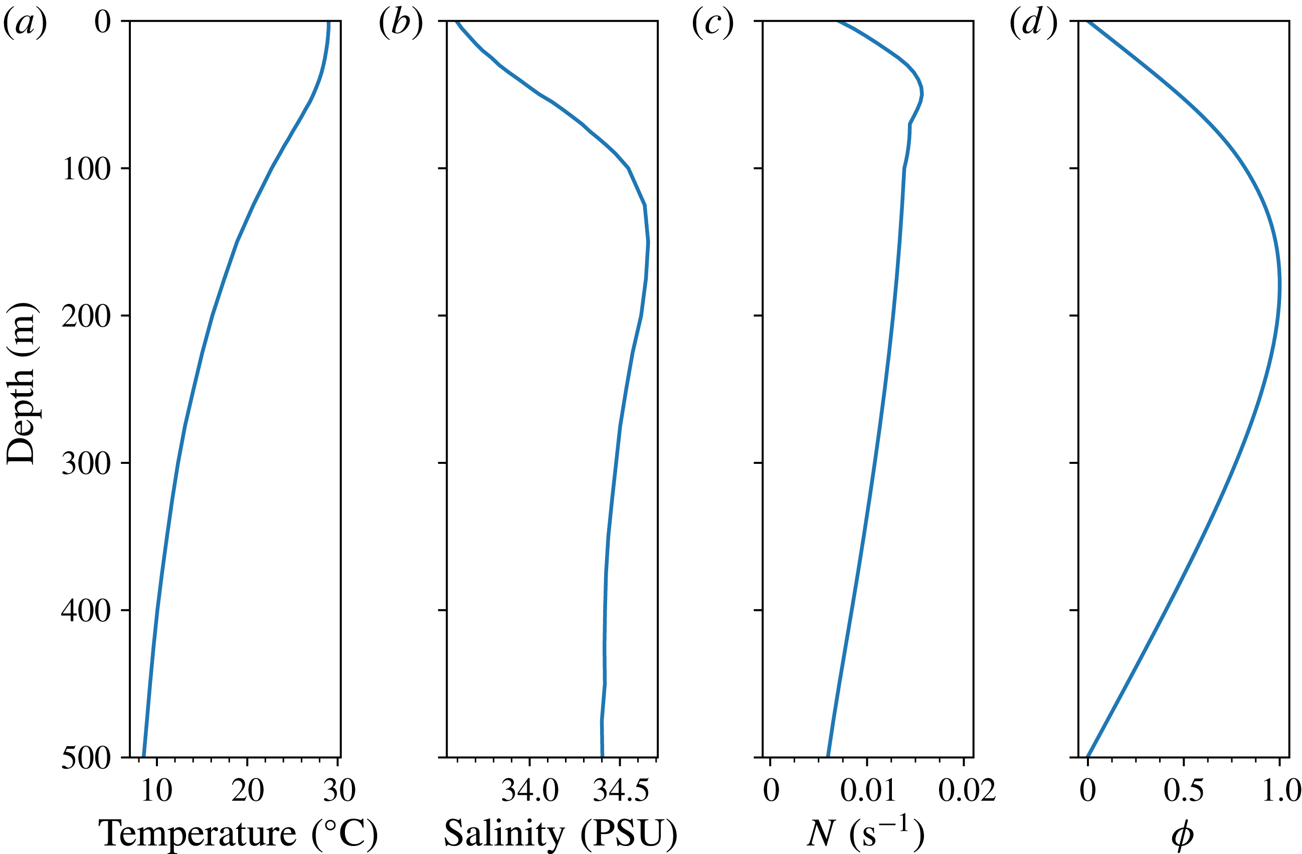
To be general, we use a density profile taken from the monthly averaged summer background temperature and salinity profiles in the SCS, taken from the World Ocean Atlas 2013, see figure 4. If another density profile is chosen, either from similar data, or from an idealized two-layer stratification, the only change would be in the coefficients
 $\unicode[STIX]{x1D707},\unicode[STIX]{x1D718}$
in the KP equation (2.9), with very similar qualitative structure. As mentioned before, observations have confirmed the occasional existence of mode-2 ISWs in the ocean, but here we confine our attention on the more commonly observed mode-1 waves, and in the KP model, we ignore any possible energy transfer between modes when the wave interactions occur. The corresponding modal function of the vKP equation shown in figure 4 indicates that initially the maximum particle displacement occurs at depth
 $h\approx 190~\text{m}$
. The negative sign of the nonlinear coefficient
 $\unicode[STIX]{x1D707}$
depicted in figure 3 implies that our leading ISWs are always depression waves, and there are no polarity changes in these simulations.
As mentioned in the Introduction, although there are a few studies of oblique internal wave interactions in the ocean, in general these investigations were not sufficiently detailed to provide a deep insight into this common but complicated phenomenon, even for the case of a flat topography. Here we use the comprehensive theory of KP solitons developed by Chakravarty & Kodama (Reference Chakravarty and Kodama2008, Reference Chakravarty and Kodama2009, Reference Chakravarty and Kodama2013) (briefly described above in § 2.2) to interpret our simulations of ISW interactions both for a constant depth and with a shoaling topography.


For EXP1, (a1–a3) are selected to exhibit the evolution of wave patterns in the case of shoaling topography at times
 $t=0,12,42$
h respectively. In contrast, (a4–a6) are for the case of constant topography at times
 $t=0,12,30$
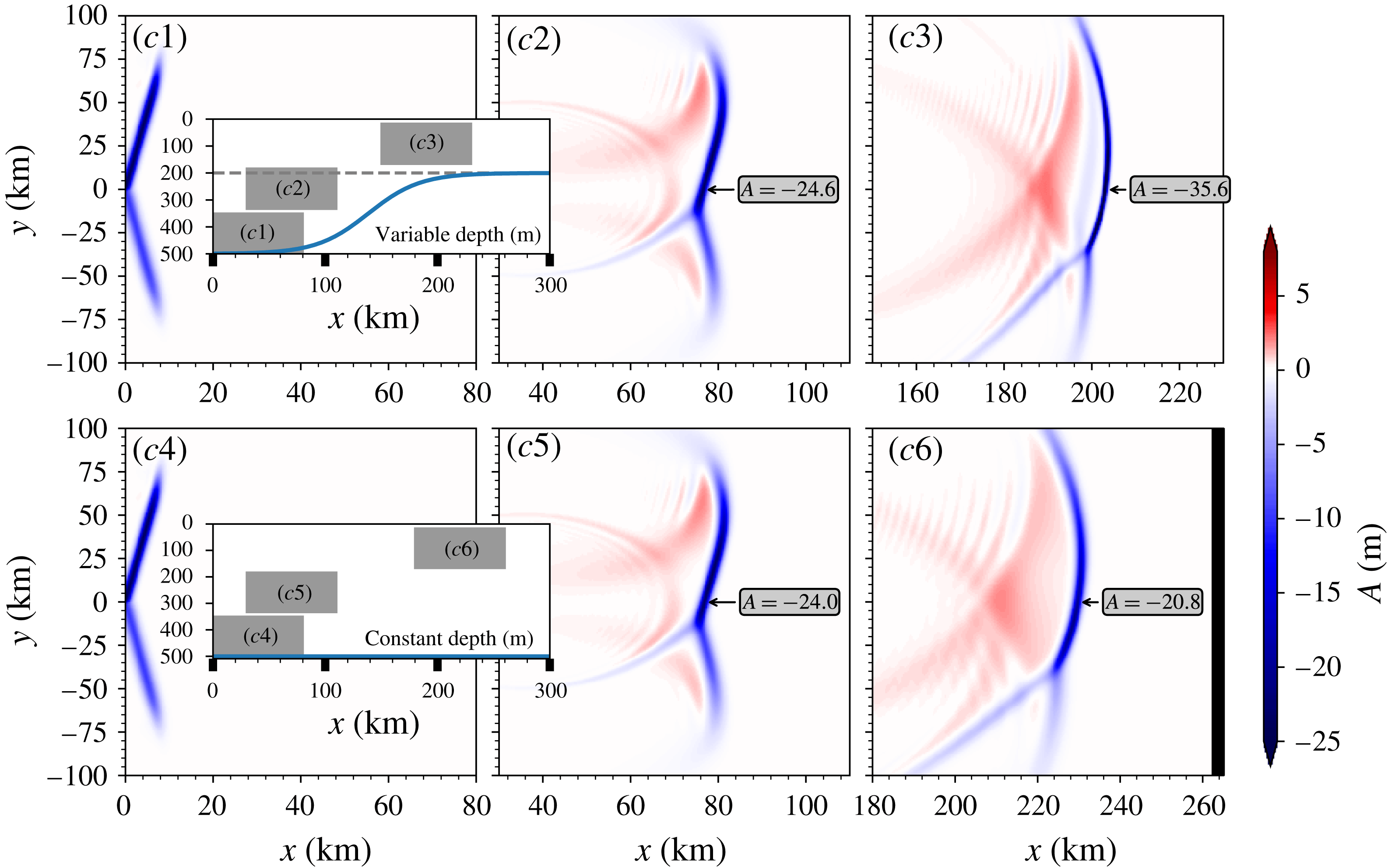
h respectively. Note that as the waves propagate faster in the constant-depth case, the snapshot is not an exact one-to-one match. The aspect ratio of every panel is the same, that is
 $x\times y=80\times 150~\text{km}$
, and the corresponding depth of every panel is indicated by insets.

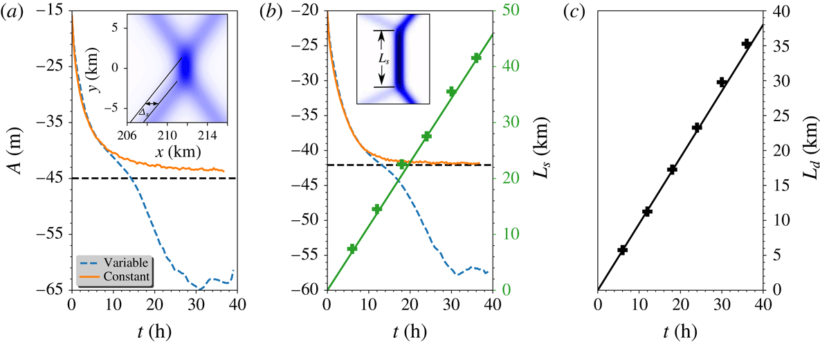
(a) In EXP1, the time series of the leading wave amplitude along
 $y=0$
for the cases of both varying and constant topography. The inset is a zoom-in in figure 5(a6). (b) In EXP2, the time series of the leading wave amplitude along
 $y=0$
for the cases of both varying and constant topography. The inset is a zoom-in in figure 7(b6). The other scale shows the length of the intermediate Mach stem
 $L_{s}$
predicted by the theory (green solid line) and the numerical simulations (green plus sign). (c) The downward distance
 $L_{d}$
varying with time in EXP3 is shown and the solid line is the theoretical result, while the plus sign is from numerical simulations.

The layout is the same as in figure 5, but for EXP2.

3.2 Experiment 1
We first examine the case, labelled as EXP1, with the initial condition of equal wave amplitudes
 $A_{1}=A_{2}=-15~\text{m}$
for the two branches and the angle
 $\unicode[STIX]{x1D6F9}_{0}=16^{\circ }$
(larger than the critical angle
 $15.1^{\circ }$
). In a constant depth of
 $h=500~\text{m}$
, this set-up is located in region 1 of figure 2 and the initial V-shape wave will asymptotically evolve to the so-called X-shape wave or O-soliton, see in figure 5(a4–a6). Subsequent to the release of the initial depression waves, two small post-interaction depression waves immediately emerge. At the same time, since the mass conservation law (2.11) has to be satisfied, waves with the opposite polarity (here elevation) are generated at the rear of the leading waves, see figure 5(a5). Then as the solution evolves, the post-interaction waves mature and eventually an X-shape wave emerges followed by a parabolic-shaped trailing wave train of opposite polarity, see figure 5(a6). A prominent feature of the developed X-shape wave is the phase shift in the interaction zone, also see figure 6, which can be interpreted through the analyses based on equation (2.14) in the transformed space (2.15). Adapting from Chakravarty & Kodama (Reference Chakravarty and Kodama2008, Reference Chakravarty and Kodama2009, Reference Chakravarty and Kodama2013), the
 $\unicode[STIX]{x1D70F}$
-function of the matured X-shape wave for the constant-coefficient equation (2.14) is represented by
 $$\begin{eqnarray}\displaystyle \unicode[STIX]{x1D70F}=1+\exp (-\unicode[STIX]{x1D6F7}_{1})+\exp (-\unicode[STIX]{x1D6F7}_{2})+B_{12}\exp (-\unicode[STIX]{x1D6F7}_{1}-\unicode[STIX]{x1D6F7}_{2}), & & \displaystyle\end{eqnarray}$$
 $$\begin{eqnarray}\displaystyle \left.\begin{array}{@{}c@{}}\unicode[STIX]{x1D6F7}_{1,2}=k_{1,2}\unicode[STIX]{x1D709}+l_{1,2}Y-\unicode[STIX]{x1D714}_{1,2}s,\quad k_{1,2}=\unicode[STIX]{x1D70E}_{2,4}-\unicode[STIX]{x1D70E}_{1,3},\\ l_{1,2}=\unicode[STIX]{x1D70E}_{2,4}^{2}-\unicode[STIX]{x1D70E}_{1,3}^{2},\quad 4\unicode[STIX]{x1D714}_{1,2}k_{1,2}=k_{1,2}^{4}+3l_{1,2}^{2},\end{array}\right\} & & \displaystyle\end{eqnarray}$$
 $$\begin{eqnarray}\displaystyle B_{12}=\frac{\unicode[STIX]{x1D6F6}^{2}-(k_{1}-k_{2})^{2}}{\unicode[STIX]{x1D6F6}^{2}-(k_{1}+k_{2})^{2}},\quad \unicode[STIX]{x1D6F6}=\frac{l_{1}}{k_{1}}-\frac{l_{2}}{k_{2}}, & & \displaystyle\end{eqnarray}$$
where the parameters have been chosen to make the phase shift of the initial incident wave to be zero. To examine this wave pattern, we take the asymptotic limits
 $\unicode[STIX]{x1D709}\rightarrow \pm \infty$
, similar to the procedure used by Miles (Reference Miles1977a
). Note that the incident
 $1$
-soliton solutions can be obtained by letting
 $\unicode[STIX]{x1D709}\rightarrow +\infty$
with either
 $\unicode[STIX]{x1D6F7}_{1}$
or
 $\unicode[STIX]{x1D6F7}_{2}$
fixed. The former limit yields one
 $1$
-soliton (2.21) with phase
 $\unicode[STIX]{x1D6F7}_{1}$
and
 $\unicode[STIX]{x1D6F7}_{0}=0$
, and the latter limit gives the other
 $1$
-soliton (2.21) with phase
 $\unicode[STIX]{x1D6F7}_{2}$
and
 $\unicode[STIX]{x1D6F7}_{0}=0$
. After the interaction, we let
 $\unicode[STIX]{x1D709}\rightarrow -\infty$
with either
 $\unicode[STIX]{x1D6F7}_{1}$
or
 $\unicode[STIX]{x1D6F7}_{2}$
fixed again. The former choice yields the
 $1$
-soliton solution (2.21) with phases
 $\unicode[STIX]{x1D6F7}_{1}$
and
 $\unicode[STIX]{x1D6F7}_{0}=\log B_{12}$
, while the latter choice yields (2.21) with phases
 $\unicode[STIX]{x1D6F7}_{2}$
and
 $\unicode[STIX]{x1D6F7}_{0}=\log B_{12}$
. This implies that the incident solitons emerge unchanged, but with a phase shift in the
 $\unicode[STIX]{x1D709}$
-direction of
 $\unicode[STIX]{x1D6E5}_{1,2}$
where
 $\exp (k_{1,2}\unicode[STIX]{x1D6E5}_{1,2})=B_{12}$
. Since
 $B_{12}>0$
to ensure the existence of the solution, the phase shifts can be positive or negative according as
 $B_{12}>1$
or
 $0<B_{12}<1$
. Since in our case the amplitudes
 $A_{1},A_{2}$
are equal, the phase shifts are the same for the upper and lower branches. In the physical variables, the theoretical estimated phase shift is
 $\unicode[STIX]{x1D6E5}_{x}=1245~\text{m}$
, slightly smaller than our numerical result
 $\unicode[STIX]{x1D6E5}_{x}=1300~\text{m}$
which emerges at the time of 6 h after the initial waves release, see figure 6. Moreover, using the modified Miles theory due to Kodama (Reference Kodama2010), Yeh et al. (Reference Yeh, Li and Kodama2010), the maximum amplitude occurring at the mid-point of the interaction is given by
 $$\begin{eqnarray}\displaystyle A_{max}=\left\{\begin{array}{@{}l@{}}\displaystyle (1+\unicode[STIX]{x1D6E4})^{2}A_{0},\quad \text{for }\unicode[STIX]{x1D6E4}<1,\\ \displaystyle \frac{4A_{0}}{1+\sqrt{1-\unicode[STIX]{x1D6E4}^{-2}}},\quad \text{for }\unicode[STIX]{x1D6E4}>1,\end{array}\right. & & \displaystyle\end{eqnarray}$$
where
 $\unicode[STIX]{x1D6E4}=\sqrt{P}\tan \unicode[STIX]{x1D6F9}/\sqrt{2A_{0}}$
and
 $A_{0}=A_{1}=A_{2}$
. It is clear that at the critical angle
 $\unicode[STIX]{x1D6F9}_{c}$
where
 $\unicode[STIX]{x1D6E4}=1$
depicted by the green dashed line in figure 2, the maximum amplitude
 $A_{max}$
can reach four times the soliton amplitude
 $A_{0}$
, as noted by Miles (Reference Miles1977a
). The estimated
 $A_{max}$
is
 $-45~\text{m}$
in our case, while the numerical result shows the value of
 $-43~\text{m}$
, see figure 6. The slight discrepancy between them is attributed to the evolution time, which is not quite long enough to let the initial V-shape wave evolve to this
 $2$
-soliton solution. Another important point is that during the interaction, the amplitudes of the initial two wave branches are unchanged, and furthermore, for the matured X-shape wave the amplitudes of the two post-interaction waves are the same as those of the initial V-shape wave, see in figure 5(a6).
When the effect of the shoaling topography is taken into account, there is a different scenario. In the deep water, the initial wave behaves like its counterpart in the constant case, but with the propagation up the slope, the front parts of the waves first experience the topographic effect, manifested as an increasing amplitude and a decreasing linear phase speed, see in figure 5(a2). The total phase speed is composed of the linear phase speed
 $c$
and the nonlinear phase speed
 $\unicode[STIX]{x1D6FC}AQ^{1/2}/3$
, and the latter has an opposite effect to that of the former, albeit the linear phase speed
 $c$
is dominant, see Yuan et al. (Reference Yuan, Grimshaw, Johnson and Chen2018b
). The incident waves begin to bend and tend to be parallel to the shore, with a decrease in the angle
 $\unicode[STIX]{x1D6F9}$
. Note that for this set-up, the critical angle
 $\unicode[STIX]{x1D6F9}_{c}=15.1^{\circ }$
, delineated by the green dashed line in figure 2, is only a little smaller than the initial angle
 $\unicode[STIX]{x1D6F9}_{0}=16^{\circ }$
. Thus due to the shoaling effect, it is possible that the evolution regime transfers from region 1 to region 2 in figure 2. Then the X-vertex wave is replaced by a merged front, called the Mach stem following Miles (Reference Miles1977b
), which emerges as a result of the resonant interaction. The length and strength of this merged front are also varying with time. We will give more details in the next section. This whole pattern continues to propagate into the shallow water and the amplitude continues to increase as
 $|\unicode[STIX]{x1D707}|^{1/3}$
(see figure 3 for
 $\unicode[STIX]{x1D707}$
) according the well-known adiabatic law determined by the conservation of wave action flux (see for instance Yuan et al. (Reference Yuan, Grimshaw, Johnson and Chen2018b
)), and meanwhile the mass of the leading depression wave, proportional to
 $|\unicode[STIX]{x1D707}|^{-1/3}$
, decreases, which results in the emergence of the trailing wave trains with the same polarity due to the mass conservation law (2.11). In the simulation, at least one trailing wave pattern with the same polarity as the leading waves is generated. But afterwards the
 $y$
-dependence has to be taken into account and the adiabatic law fails. Figure 6 shows the amplitude of the leading wave at the centre
 $y=0$
, and eventually after the waves propagates onto the flat shelf it is more than four times larger than the initial wave. Note that as Tsuji & Oikawa (Reference Tsuji and Oikawa2007) pointed out, the resonance and hence the amplification of the wave amplitude at the mid-point of the interaction can be suppressed to some extent when it approaches a critical depth where the quadratic coefficient
 $\unicode[STIX]{x1D707}$
(or
 $\unicode[STIX]{x1D6FC}$
) approaches zero. In figure 5(a3), we see that the interaction zone does not have much influence on the evolution of the initial two branches, which still behave approximately like the adiabatic shoaling process predicted by the KdV theory. In contrast, the evolution of the post-interaction waves are highly affected by the interaction, see figure 5(a3). The post-interaction waves adjacent to the interacted merged front have a relatively smaller amplitude compared with the neighbouring waves along the wave crest. This could be due to the conservation of the wave action flux (2.12), since around the junction of the merged front and the post-interaction waves, a large
 $y$
-gradient is needed to compensate the increase of the energy induced by the increasing amplitude. This indicates the failure of the KdV adiabatic law. After the waves propagate onto the flat shelf, the linear phase speed is the same for all waves, however the nonlinear phase speed
 $\unicode[STIX]{x1D6FC}AQ^{1/2}/3$
is dependent on the wave amplitude, so the post-interaction wave branches will be curved with the larger waves moving faster.
3.3 Experiment 2
Next we set the initial wave amplitudes
 $A_{1}=A_{2}=-20~\text{m}$
and the angle
 $\unicode[STIX]{x1D6F9}_{0}=8^{\circ }$
(smaller than the critical angle
 $17.3^{\circ }$
), which is pattern (b) in figure 2 in the constant depth
 $h=500~\text{m}$
water; this set-up is labelled as EXP2. At the initial stage, the evolution is almost the same as in EXP1, which is partly characterised by the radiation of two post-interaction waves and a parabolic-shaped wave train of opposite polarity. The essential difference is the generation of a Mach stem in the middle of the initial two wave branches and its length is increasing with time. Eventually the pattern asymptotically converges to the (3142)-type solutions in Chakravarty & Kodama (Reference Chakravarty and Kodama2008, Reference Chakravarty and Kodama2009, Reference Chakravarty and Kodama2013). The
 $\unicode[STIX]{x1D70F}$
-function in the transformed space (2.15) is given by
 $$\begin{eqnarray}\displaystyle \unicode[STIX]{x1D70F}=E(1,3)+bE(1,4)+aE(2,3)+abE(2,4)+cE(3,4), & & \displaystyle\end{eqnarray}$$
where
 $E(i,j)=(\unicode[STIX]{x1D70E}_{j}-\unicode[STIX]{x1D70E}_{i})\exp (\unicode[STIX]{x1D703}_{i}+\unicode[STIX]{x1D703}_{j})$
, the phase
 $\unicode[STIX]{x1D703}_{n},n=1,2,3,4$
is defined in equation (2.18), and
 $a,b,c>0$
are parameters which determine the location of the solitons. Using the same method of asymptotic limits introduced before, when
 $\unicode[STIX]{x1D709}\rightarrow +\infty ,Y\rightarrow +\infty$
, the soliton, see analogously the right upper branch in figure 7, can be obtained from the balance between the terms
 $bE(1,4)$
and
 $cE(3,4)$
, which yields the 1-soliton solution (2.21) with the amplitude
 $\unicode[STIX]{x1D6EC}_{13}=(\unicode[STIX]{x1D70E}_{3}-\unicode[STIX]{x1D70E}_{1})^{2}/2$
, the phase
 $\unicode[STIX]{x1D6F7}_{13}=\unicode[STIX]{x1D703}_{3}-\unicode[STIX]{x1D703}_{1}$
and the phase shift
 $$\begin{eqnarray}\displaystyle \unicode[STIX]{x1D6F7}_{013}=\ln \left\{\frac{(\unicode[STIX]{x1D70E}_{4}-\unicode[STIX]{x1D70E}_{1})}{(\unicode[STIX]{x1D70E}_{4}-\unicode[STIX]{x1D70E}_{3})}\frac{b}{c}\right\}. & & \displaystyle\end{eqnarray}$$
Similarly, when
 $\unicode[STIX]{x1D709}\rightarrow +\infty ,Y\rightarrow -\infty$
(the right lower branch), the soliton is given by expression (2.21) with the amplitude
 $\unicode[STIX]{x1D6EC}_{24}=(\unicode[STIX]{x1D70E}_{4}-\unicode[STIX]{x1D70E}_{2})^{2}/2$
, the phase
 $\unicode[STIX]{x1D6F7}_{24}=\unicode[STIX]{x1D703}_{4}-\unicode[STIX]{x1D703}_{2}$
and the phase shift
 $$\begin{eqnarray}\displaystyle \unicode[STIX]{x1D6F7}_{024}=\ln \left\{\frac{(\unicode[STIX]{x1D70E}_{3}-\unicode[STIX]{x1D70E}_{2})}{(\unicode[STIX]{x1D70E}_{4}-\unicode[STIX]{x1D70E}_{3})}\frac{a}{c}\right\}. & & \displaystyle\end{eqnarray}$$
On the other hand as
 $\unicode[STIX]{x1D709}\rightarrow -\infty$
the dominant terms in (3.5) are either the pair
 $E(1,3),E(1,4)$
yielding a
 $1$
-soliton with the amplitude
 $\unicode[STIX]{x1D6EC}_{34}=(\unicode[STIX]{x1D70E}_{4}-\unicode[STIX]{x1D70E}_{3})^{2}/2$
and the phase
 $\unicode[STIX]{x1D6F7}_{34}=\unicode[STIX]{x1D703}_{4}-\unicode[STIX]{x1D703}_{3}$
(the left upper branch) or the pair
 $E(1,3),E(2,3)$
yielding a second
 $1$
-soliton with the amplitude
 $\unicode[STIX]{x1D6EC}_{12}=(\unicode[STIX]{x1D70E}_{2}-\unicode[STIX]{x1D70E}_{1})^{2}/2$
and the phase
 $\unicode[STIX]{x1D6F7}_{12}=\unicode[STIX]{x1D703}_{2}-\unicode[STIX]{x1D703}_{1}$
(the left lower branch). They have the respective phase shifts
 $$\begin{eqnarray}\displaystyle \unicode[STIX]{x1D6F7}_{034}=\ln \left\{\frac{(\unicode[STIX]{x1D70E}_{3}-\unicode[STIX]{x1D70E}_{1})}{(\unicode[STIX]{x1D70E}_{4}-\unicode[STIX]{x1D70E}_{1})}\frac{1}{b}\right\},\quad \unicode[STIX]{x1D6F7}_{012}=\ln \left\{\frac{(\unicode[STIX]{x1D70E}_{3}-\unicode[STIX]{x1D70E}_{1})}{(\unicode[STIX]{x1D70E}_{3}-\unicode[STIX]{x1D70E}_{2})}\frac{1}{a}\right\}. & & \displaystyle\end{eqnarray}$$
Importantly, the total phase shift is locked for all values of
 $a,b,c>0$
, as Miles (Reference Miles1977a
) pointed out,
 $$\begin{eqnarray}\displaystyle \unicode[STIX]{x1D6F7}_{013}+\unicode[STIX]{x1D6F7}_{034}=\unicode[STIX]{x1D6F7}_{024}+\unicode[STIX]{x1D6F7}_{012}. & & \displaystyle\end{eqnarray}$$
The generation of the Mach stem is a consequence of the resonance between the upper right branch and the upper left branch, as well as between the lower right and the lower left branch. Note that the Mach stem can be represented by the soliton solution (2.21) with the amplitude
 $\unicode[STIX]{x1D6EC}_{14}=(\sqrt{2\unicode[STIX]{x1D6EC}_{0}}+\tan \unicode[STIX]{x1D6F9}_{0})^{2}/2$
and the phase
 $\unicode[STIX]{x1D6F7}_{14}=\unicode[STIX]{x1D703}_{4}-\unicode[STIX]{x1D703}_{1}$
. Then the length of the stem
 $L_{s}$
can be expressed as
 $L_{s}=(\sqrt{2\unicode[STIX]{x1D6EC}_{0}}-\tan \unicode[STIX]{x1D6F9}_{0})s$
, which is obtained by examining the location of the intersection point between the stem and the initial upper left branch.
Since in the present case, the amplitudes of the initial two branches are the same, that is
 $\unicode[STIX]{x1D6EC}_{13}=\unicode[STIX]{x1D6EC}_{24}=A_{0}/P$
where
 $A_{0}=A_{1,2}$
, and the initial wave passes through the origin
 $\unicode[STIX]{x1D709}=Y=0$
at time
 $s=0$
, the phase shift
 $\unicode[STIX]{x1D6F7}_{013}=\unicode[STIX]{x1D6F7}_{024}=0$
, fixes two values from
 $a,b,c$
and only one free parameter is left. In the physical space, through the transformation (2.8), the estimated amplitude of the post-interaction wave is
 $-4~\text{m}$
, well matches with the numerical result, see figure 7(b6). The length of the stem
 $L_{s}$
is shown in figure 6(b), and there is a remarkable agreement between the theory and numerical simulations. In addition, from equation (3.4), the amplification factor (relative to the initial wave amplitude) is
 $(1+\unicode[STIX]{x1D6E4})^{2}=2.1$
since
 $\unicode[STIX]{x1D6E4}=0.45<1$
, and again a very good consistency with the numerical results, see figure 6.
The evolution scenario over the shoaling topography is similar to that in EXP1, except for the evolution of the intermediate Mach stem. As the solution evolves, the amplitude of the stem is not constant either along
 $y$
-sections or along the stem itself, in contrast to the eventual constant amplitude in the flat bottom case. Figure 6 shows the increasing amplitude of the leading wave along
 $y=0$
. The magnification of the wave amplitude in the interaction zone is not as efficient as that in EXP1, since here it increases approximately once, smaller than the twice in EXP1. Note that here the varying topography is
 $y$
-independent, thus any transverse effect must enter the equation through the spreading term
 $\unicode[STIX]{x1D718}U_{yy}$
in the vKP equation (2.9). Since the two initial wave branches are oblique, the front parts experience the topographic effect and consequently deform earlier than the rear parts. Then this discrepancy along the branches induces a complicated modulation in both the
 $X$
direction due to the mass conservation law and further in the
 $y$
direction to respond to the variations in the
 $X$
direction, as the wave action flux must be conserved. In figure 7(b3), we find that the stem has a very special structure. As we mentioned before, in general, the waves with larger amplitude propagate faster, however figure 7(b3) shows that along the stem, the wave at
 $y=0$
section with smaller amplitude surprisingly propagates faster than its larger neighbouring waves. This indicates a profound topographic effect on wave–wave interactions. Also note that after time
 $t=42h$
(see figure 7
b3), the whole wave pattern will propagate onto the flat shelf, and if the flat shelf is long enough, then the stem is likely to become parallel to the shore. However, we are not able to verify this here, as our computational domain is not sufficiently long.
The layout is the same as in figure 5, but for EXP3.

3.4 Experiment 3
In EXP2, in the case of constant depth, we showed that the resonant interaction between the initial wave and the post-interaction wave generated a third wave (Mach stem). In this section, we will examine this further. In figure 2, patterns (c,d) have the same dynamical features, both of which need two initial branches with different amplitudes. Here we select pattern (c) with the initial condition
 $A_{1}=-25~\text{m}$
,
 $A_{2}=-10~\text{m}$
and the angle
 $\unicode[STIX]{x1D6F9}_{0}=3.67^{\circ }$
satisfying the critical relation
 $\sqrt{2\unicode[STIX]{x1D6EC}_{1}}-\sqrt{2\unicode[STIX]{x1D6EC}_{2}}=2\tan \unicode[STIX]{x1D6F9}_{0}$
(the thick solid line in figure 2). This case is labelled as EXP3. Note that as shown in our figure 1 and also in Chen et al. (Reference Chen, Liu, Wang and Hsu2011), this pattern has been observed in the SCS. Here the
 $\unicode[STIX]{x1D70F}$
-function of the developed wave pattern, see in figure 8(c6), is
 $$\begin{eqnarray}\displaystyle \unicode[STIX]{x1D70F}=1+\exp (-\unicode[STIX]{x1D6F7}_{1})+\exp (-\unicode[STIX]{x1D6F7}_{2}). & & \displaystyle\end{eqnarray}$$
As
 $\unicode[STIX]{x1D709}\rightarrow +\infty$
, this describes two incident solitons with respective phases as defined in (3.2). But as
 $\unicode[STIX]{x1D709}\rightarrow -\infty$
, this describes the generation of a third resonant soliton with phase
 $\unicode[STIX]{x1D6F7}_{3}=k_{3}x+l_{3}y-\unicode[STIX]{x1D714}_{3}t$
, where
 $k_{3},l_{3},\unicode[STIX]{x1D714}_{3}$
satisfy the resonance conditions,
 $$\begin{eqnarray}\displaystyle \left.\begin{array}{@{}c@{}}\displaystyle \unicode[STIX]{x1D714}_{3}=\unicode[STIX]{x1D714}_{1}-\unicode[STIX]{x1D714}_{2},\quad k_{3}=k_{1}-k_{2},\quad l_{3}=l_{1}-l_{2},\\ \displaystyle 4\unicode[STIX]{x1D714}_{i}k_{i}=k_{i}^{4}+3l_{i}^{2},\quad i=1,2,3.\end{array}\right\} & & \displaystyle\end{eqnarray}$$
Upon noting that
 $\unicode[STIX]{x1D6F7}_{3}=\unicode[STIX]{x1D6F7}_{1}-\unicode[STIX]{x1D6F7}_{2}$
, fixing
 $\unicode[STIX]{x1D6F7}_{3}$
and taking the limit
 $\unicode[STIX]{x1D709}\rightarrow -\infty$
yields
 $$\begin{eqnarray}\displaystyle \unicode[STIX]{x1D70F}\sim 1+\exp (-\unicode[STIX]{x1D6F7}_{3}),\quad u\sim \frac{k_{3}^{2}}{2}\,\text{sech}^{2}\left(\frac{\unicode[STIX]{x1D6F7}_{3}}{2}\right). & & \displaystyle\end{eqnarray}$$
Thus the amplitude of the third wave is
 $k_{3}^{2}/2$
, which is
 $-3.4~\text{m}$
using our physical variables, very close to the numerical result
 $-3.3~\text{m}$
, see in figure 8(c6). From (2.22), the propagation speed is related to the amplitude and angle. In this set-up two branches are of the same inclination but different initial amplitudes, and it follows that the intersection point will move downward with respect to
 $y=0$
based on a simple geometric relation. In the transformed space (2.15), the downward distance is
 $$\begin{eqnarray}\displaystyle L_{d}=\frac{(\unicode[STIX]{x1D6EC}_{2}-\unicode[STIX]{x1D6EC}_{1})s}{4\tan \unicode[STIX]{x1D6F9}_{0}}, & & \displaystyle\end{eqnarray}$$
which is confirmed by our numerical simulations shown in the physical space, see figure 6.
It is clear that in this case, there are no mechanisms that can boost the amplitude at the intersection point, which is different from the previous two cases. When the topographic effect is considered, as before, a wave train of opposite polarity, together with a second wave pattern with the same polarity, follows the leading wave pattern, see in figure 8(c3). In this case, the curvature of the leading two wave branches is significant, since the absence of a resultant large-amplitude intermediate wave in the interaction zone seems to suppress the transverse modulation. Thus the evolution can be partly predicted by the KdV theory, see for instance Grimshaw, Pelinovsky & Talipova (Reference Grimshaw, Pelinovsky and Talipova2007), Grimshaw et al. (Reference Grimshaw, Pelinovsky, Talipova and Kurkina2010).
3.5 Short along-crest width
The aforementioned cases are such that the initial waves fill the whole transverse domain and indeed this set-up can be of some practical interest. In a realistic ocean, although the along-crest width can be as long as several hundred kilometres, in some circumstances, it is permissible to focus only on central parts, where the effect induced by the wave edges is considered unimportant. Nevertheless, since the real ocean can be regarded as open for ISWs, the case in which waves can propagate freely in the transverse direction should also be examined, which amounts here to considering a wave with a short along-crest width propagating in a large domain. In this sub-section we will examine this issue. The set-ups are the same as those in the previous three cases, except that a
 $y$
-envelope
 $\text{ENV}(y)$
(2.25) is imposed on the initial wave. Figures 9–11 show the evolution scenarios. For each figure, the horizontal view is quite similar qualitatively, which is presumably indicative of the significance of the spreading effect in the transverse direction. However closer scrutiny shows that topographic effect does still modulate the amplitude of the waves.
We consider the case of constant water depth first. After the initial launch, similar post-interaction waves and their consequent trailing opposite wave trains emerge just as in EXP1–EXP3. However, here due to the spread in the
 $y$
direction, then another pair of wave trains of opposite polarity arises behind the two leading branches as a consequence of mass conservation. Note that the dispersion relation of the KP equation (2.14) for a linear wave
 $\unicode[STIX]{x1D6F7}=\exp (\text{i}k\unicode[STIX]{x1D709}+\text{i}lY-\text{i}\unicode[STIX]{x1D714}s)$
with frequency
 $\unicode[STIX]{x1D714}$
and wavenumbers
 $k,l$
is given by
 $$\begin{eqnarray}\displaystyle \unicode[STIX]{x1D714}=-\frac{k^{3}}{4}+\frac{3l^{2}}{4k}, & & \displaystyle\end{eqnarray}$$
from which the group velocity of the wave is
 $$\begin{eqnarray}\displaystyle C_{g\unicode[STIX]{x1D709}}=-\frac{3}{4}\left(k^{2}+\frac{l^{2}}{k^{2}}\right),\quad C_{gY}=\frac{3l}{2k}. & & \displaystyle\end{eqnarray}$$
The (always) negative sign of the group speed
 $C_{g\unicode[STIX]{x1D709}}$
in the
 $\unicode[STIX]{x1D709}$
direction implies that any small perturbation must propagate in the negative
 $\unicode[STIX]{x1D709}$
direction. Thus in the physical space, any generated small-amplitude wave trains will appear behind the leading waves and gradually detach from them. Then the spreading effect keeps expanding the waves in the
 $y$
-direction at the cost of decreasing wave amplitude from the periphery gradually up to the centre. As mentioned, the nonlinear phase speed is related to the amplitude, so as a result, overall the initial two oblique waves become parallel to the shore, and eventually they merge into one large leading wave, followed by the post-interaction waves and wave trains of opposite polarity. This wave pattern continues to propagate, but the spreading effect radiates the energy away from the calculation domain.
When the topographic effect is taken into consideration, the spreading effect is still dominant, but at the same time, the amplitude is enlarged by the shoaling process, compared with that in the constant water depth. Especially, the difference in the eventual merged leading wave in figure 9 is appreciable, which can be ascribed to the topographic effect, see also figure 5.
The layout is the same as in figure 5 but the aspect ratio of every panel is
 $x\times y=80\times 200~\text{km}$
here. The set-up is the same as that in EXP1, except that an envelope is imposed on the initial V-shape wave.

The layout is the same as in figure 5 but the aspect ratio of every panel is
 $x\times y=80\times 200~\text{km}$
here. The set-up is the same as that in EXP2, except that an envelope is imposed on the initial V-shape wave.

The layout is the same as in figure 5 but the aspect ratio of every panel is
 $x\times y=80\times 200~\text{km}$
here. The set-up is the same as that in EXP3, except that an envelope is imposed on the initial V-shape wave.
4 Conclusion
Motivated by the observations reported in Chen et al. (Reference Chen, Liu, Wang and Hsu2011), Wang & Pawlowicz (Reference Wang and Pawlowicz2012), Xue et al. (Reference Xue, Graber, Romeiser and Lund2014) and many SAR images, we have examined three cases of oblique internal wave–wave interactions using a V-shape wave consisting of two branches of ISWs as the initial condition.
In constant-depth water, when the along-crest width is relatively short compared with the domain of interest, the spreading effect in the transverse direction is dominant, which eventually destroys the initial structure of two oblique waves and leads to the emergence of one merged leading wave followed by wave trains of opposite polarity. However, if we consider the case when the initial waves fill the whole transverse domain, then the evolution scenario can be categorised into six types depending on the amplitude and slope of each wave branch. From the six types of behaviour shown in figure 2, patterns (c,d), and patterns (e,f) have the same dynamical features. The upper bifurcation angle
 $\unicode[STIX]{x1D6F9}_{c}$
distinguishing pattern (a,b) is described by
 $\sqrt{2\unicode[STIX]{x1D6EC}_{1}}+\sqrt{2\unicode[STIX]{x1D6EC}_{2}}=2\tan \unicode[STIX]{x1D6F9}_{c}$
(the green dashed line in figure 2). Here the water depth is
 $h=500~\text{m}$
, motivated by the depth of the continental shelf in the SCS, and then choosing the amplitudes of the two branches to be
 $A_{1}=A_{2}=100~\text{m}$
, the critical angle is
 $\unicode[STIX]{x1D6F9}_{c}=35^{\circ }$
. If we were to simplify our continuous stratification to a two-layer structure, using the modal function shown in figure 4, the thickness of the upper layer could be estimated as
 $h_{1}\approx 190~\text{m}$
. Thus in this situation the nonlinearity parameter
 $A_{1}/h_{1}=0.53$
indicates strongly nonlinear ISWs and may be outside the weakly nonlinear assumption of the KP equation. This suggests that for most cases of two waves interacting on the shelf of the SCS, the critical angle
 $\unicode[STIX]{x1D6F9}_{c}$
will be much smaller than
 $35^{\circ }$
. But we note that the Dongsha Atoll, located at approximately
 $116^{\circ }45^{\prime }$
E,
 $20^{\circ }40^{\prime }$
N near the continental shelf (see figure 1), can cut one oncoming large ISW into two oblique fragments (see Guo & Chen Reference Guo and Chen2014), which, along with the multiple potential generation sites for ISWs, suggests that the patterns in figure 2 may not be very rare in the SCS. However, patterns (e,f) are not robust and are less likely to be observed.
Both patterns (a,b) contain an intermediate zone characterised by relatively large-amplitude waves and in our specific cases these are three times as large as the initial waves in pattern (a) and twice the initial waves in pattern (b). For pattern (a), there is a phase shift in the interaction zone and this zone is neither expanding nor shrinking with time, while for pattern (b), the intermediate area is an uniform stem whose transverse length is linearly increasing with time. The occurrence of this stem is a superposition of the interaction emerging between upper two wave branches and that arising between lower two waves and this was further examined in pattern (c), in which a third post-interaction wave is apparent.
The effect of shoaling topography modulates the wave field, primarily manifested as an augmented leading depression wave followed by parabolic-shaped wave trains of opposite polarity and secondary wave trains of the same polarity, which is induced by mass conservation in the
 $X$
direction. As waves propagate up the shoaling topography, their phase speeds decrease. Then the front parts of the leading waves undergo the topographic effect earlier than the rear parts, which overall results in decreasing angles of the oblique leading wave branches. This feature can make the evolution pattern move from one region to another as described in figure 2. Also, the post-interaction wave branches have a special structure because the amplitudes and discrepancies along the branches induce curvatures with larger waves propagating faster. When the along-crest width is short, the wave amplitude is amplified by the shoaling process, although the spreading effect in the transverse direction is still dominant, as for constant depth. Since here the generated wave trains are of small amplitude, they can be treated approximately as small linear perturbation. Then the dispersion relation for the KP equation shows that these small perturbations have a negative group velocity in the
 $X$
direction and detach from the leading waves, which is affirmed by our numerical simulations.
It is clear that for these internal wave–wave interactions, the relationships between amplitude and angle are very significant. We note that the existing observations on this phenomena are mainly from SAR imagery and aerial photography and sometimes it is just one snapshot rather than sequential images. Here we caution that it may not be very reliable to interpret just one observed wave pattern from an instantaneous image, and it is desirable to obtain also information of the whole water column.
Acknowledgements
C.Y. was supported by the Chinese Scholarship Council and UCL Dean’s prize. R.G. was supported by the Leverhulme Trust through the award of a Leverhulme Emeritus Fellowship. Z.W. was supported by the National Natural Science Foundation of China (no. 11772341) and Strategic Priority Research Program of the Chinese Academy of Sciences (no. XDB22040203).