Nomenclature
- AR
-
aspect ratio
-
 ${C_L}$
-
lift coefficient
-
${C_D}$
-
drag coefficient
-
${C_m}$
-
pitch moment coefficient
-
${C_m}0$
${0^ \circ }\alpha $
-
pitch moment coefficient
- CCD
-
central composite design
- CEM
-
computational electron magnetics
- CFD
-
computational fluid dynamics
- DOE
-
design of experiment
- FEA
-
finite element analysis
- FFD
-
free form deformation
- GCPSO
-
guarantee convergence particle swarm optimisation
- GDA
-
gradient descent algorithm
- L/D
-
lift to drag ratio
- MALE
-
medium altitude long endurance
- PO
-
physical optics
- RCS
-
radar cross section
- RSM
-
response surface methodology
- SST
-
shear stress transport
- UAV
-
unmanned aerial vehicle


Greek symbol
-
$\alpha $
-
angle-of-attack
-
$\lambda $
-
sweep angle
-
${\rm{\gamma }}$
-
dihedral angle
-
$\rho $
-
density
-
$\tau $
-
stress


1.0 Introduction
Unmanned aerial vehicles (UAV) are an effective tool to counter targets in the designated enemy territory without the risk of losing human life in the modern era of hybrid warfare. These UAVs must be designed with low radar observability so that they can perform their mission without the risk of being detected. The shape of the aerial vehicle has a great influence on the wave scattering behaviour of the aircraft/UAV. These shape changes are not synonymous with the RCS of the aircraft only but also affect its aerodynamic characteristics. One shape change that is beneficial for one aspect can be detrimental to the other. Thus, a balanced approach is required in this multidisciplinary design problem to improve the aerodynamics of the aircraft while keeping a lower radar signature.
The solution to the dilemma of the aircraft designer, involving maximising aerodynamic efficiency and reducing radar signature while adhering to the timeline constraints in the aerospace industry, can be performed utilising various optimisation techniques. These techniques combine computational electromagnetics (CEM) theory, computational fluid dynamics (CFD) theory and an optimisation design approach into one consolidated design tool. In this regard, many researchers have worked on various optimisation techniques for developing tools that can design a balanced Aero-RCS aircraft model [Reference Lian, Oyama and Liou1]. The general approach adopted by researchers is basically focused on two optimisation models:
-
1. Gradient-free model
-
2. Gradient-based model
In the gradient-free model domain, published research work such as Wu Di et al. [Reference Wu, Long, Li, Jiang and Huang2] used an aero-stealth coupled optimisation method for a high aspect ratio wing aerofoil. It utilises enhanced adaptive response surface equations for wing optimisation at a lower computational cost. Similarly, Zhou et al. [Reference Zhou, Huang and Yi3] proposed an optimisation method based on the Pareto solution for reducing aerodynamic drag and the RCS of a helicopter rotor without degrading aerodynamic characteristics. The aerodynamics problem is solved using Navier-Stokes equations, while the RCS value is calculated by physical optics (PO) techniques. In Ref. [Reference Zhang, Lie, Chen, Shen, Jiao and Yuan4], the author employed a multidisciplinary design optimisation approach considering UAV radar signature and flight trajectory for design optimisation.
In the preceding paragraph, all of the referred work employed gradient-free optimisation design algorithms for the Aero-RCS coupled design optimisation problem. Although this optimisation technique produces results/data points closer to the optimal value, achieving this accuracy requires a large number of iterations. This significantly increases the computational requirements for a simple task. In this context, gradient-based optimisation techniques tend to converge quickly to the optimal values with a minimum number of iterations and function evaluations [Reference Halleröd, Ericsson and Bondeson5]. Although work has been done in this context before [Reference Li, Bai, Li, Meng, Liu and Chen6,Reference Liu, Song, Han and Wang7], utilising various gradient-based optimisation techniques for balanced Aero-RCS design, these studies have been limited to smaller design variables.
Our work focuses on utilising a modified gradient-based optimiser approach for multiple-variable-based Aero-RCS design using a radial function-based approach, employing CFD and PO solvers. Furthermore, different design constraints and weight factors are introduced, and their effects are evaluated. For validation of results, the optimised model is evaluated via simulations and experimental testing for RCS in anechoic chamber.
The highlights of this work are as follows:
-
• Gradient-based algorithm approach for Aero-RCS optimisation
-
• Multi-variable, multi-constraint optimisation approach
-
• High-fidelity simulation analysis of the optimised result and experimental testing of the optimised model
2.0 Literature review
The optimisation of aerodynamics and RCS in UAVs has garnered substantial attention due to the dual need for enhanced performance and stealth capabilities. Various researchers have explored optimisation techniques, particularly the gradient descent algorithm (GDA), to address these challenges, yielding significant advancements in UAV design.
Champasak et al. [Reference Champasak, Panagant, Pholdee, Bureerat and Riza Yildiz8] utilised a meta-heuristic to optimise drag and lift coefficients of fixed-wing UAVs. By integrating aerodynamic analyses using the vortex lattice method and empirical estimations, their approach demonstrated superior performance in reducing drag and enhancing lift. Similarly, Zhu et al. [Reference Zhu, Guo and Ma9] focused on optimising barrel-launched UAV wings equipped with multiple control surfaces. Using a surrogate model and a multi-objective genetic algorithm, their method achieved a 28.36% improvement in lift-to-drag ratio and a 164.29% enhancement in control torques, emphasising the integration of aerodynamic optimisation with control capabilities. Lee et al. [Reference Lee, Gonzalez, Srinivas and Periaux10] proposed a hybrid framework combining GDA with evolutionary algorithms to optimise aerofoil sections and wing shapes. This approach improved aerodynamic efficiency and reduced radar visibility, demonstrating the versatility of gradient-based methods in multi-objective optimisation. Wu et al. [Reference Wu, Long, Li, Jiang and Huang2] introduced an aero-structure-stealth optimisation framework that coupled CFD, finite element analysis (FEA) and CEM. Their study validated the ability to simultaneously enhance aerodynamic performance and reduce RCS. Zhou et al. [Reference Zhou, Huang and Yi3] applied Pareto-based optimisation to reduce aerodynamic noise and RCS in helicopter rotors. Leveraging unstructured grid meshing and Navier-Stokes equations, their method achieved significant reductions in both metrics, highlighting the synergy between stealth and aerodynamic goals.
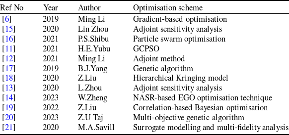
In another study, Li et al. [Reference Li, Bai, Li, Meng, Liu and Chen6] explored optimisation strategies for flying-wing aircraft using gradient-based methods combined with free-form deformation (FFD) and radial basis functions (RBF). Their approach effectively balanced aerodynamic and stealth improvements. Yubo et al. [Reference Yubo, Qingzhen and Xiang11] focused on serpentine nozzle designs, achieving an 83.33% reduction in RCS alongside aerodynamic enhancements using the guarantee convergence particle swarm optimisation (GCPSO) algorithm. Similarly, Li et al. [Reference Li, Chen, Feng, Qu and Bai12] employed an adjoint method for aero-stealth optimisation, optimising drag and RCS metrics while improving computational efficiency. Zhou et al. [Reference Zhou, Huang, Gao and Zhang13] advanced this concept by using adjoint sensitivity analysis to refine three-dimensional aerodynamic and stealth designs. Recent studies have also incorporated multifidelity models to optimise UAV designs. Liu et al. [Reference Liu, Song, Han and Wang7] introduced a modified multifidelity surrogate model that enhanced computational efficiency while balancing aerodynamic and stealth objectives. Zhang et al. [Reference Zhang, Gao, Wang and Xia14] used a niching-based adaptive space reconstruction method to address multimodal design spaces, effectively balancing aerodynamic and stealth requirements. An overview of the literature review is provided in Table 1.
Summary of optimisation schemes used in recent UAV design studies

Despite these advancements, significant gaps remain in current research. While numerous studies have explored aerodynamic or stealth optimisation separately, the combined Aero-RCS optimisation for medium-altitude long-endurance (MALE) UAVs remains unaddressed. Furthermore, no study has verified these results experimentally or through high-fidelity simulations. This gap underscores the need for a comprehensive framework that simultaneously optimises aerodynamics and RCS for MALE UAVs while validating the outcomes. This research aims to address this critical gap by developing and verifying an integrated optimisation methodology, providing a robust solution for next-generation UAV design challenges.
3.0 Methodology
3.1 Problem formulation
The primary objective of this optimisation study is to enhance the aerodynamic performance and stealth characteristics of a UAV. Specifically, the goal is to maximise the overall lift coefficient (
 ${C_L}$
) while simultaneously minimising both the overall and frontal RCS. The design variables selected for this optimisation include critical aircraft geometry parameters: the wing aspect ratio (
 $A{R_{{\rm{wing}}}}$
), wing sweep angle (
 $Swe{p_{{\rm{wing}}}}$
), tail aspect ratio (
 $A{R_{{\rm{tail}}}}$
) and tail dihedral angle (
 $Dihedra{l_{{\rm{tail}}}}$
). These parameters are known to influence both aerodynamic efficiency and radar signature, making them essential for the multi-objective optimisation approach.
The objective function for this optimisation is defined as:
 \begin{align*}f\left( {\bf{x}} \right) = - \frac{{{C_{{L_{{\rm{max}}}}}}}}{{{C_{{L_{{\rm{max}}}}}}\left( {{\rm{Max}}} \right)}} + \frac{{{\rm{RC}}{{\rm{S}}_{{\rm{overall}}}}}}{{{\rm{RC}}{{\rm{S}}_{{\rm{overall}}}}\left( {{\rm{Max}}} \right)}} + \frac{{{\rm{RC}}{{\rm{S}}_{{\rm{frontal}}}}}}{{{\rm{RC}}{{\rm{S}}_{{\rm{frontal}}}}\left( {{\rm{Max}}} \right)}}\end{align*}
where:
-
•
${C_L}$
represents the overall lift coefficient of the UAV. -
•
${\rm{RC}}{{\rm{S}}_{{\rm{overall}}}}$
and
${\rm{RC}}{{\rm{S}}_{{\rm{frontal}}}}$
are the total and frontal radar cross-sections, respectively. -
•
${\bf{x}}$
is the vector of design variables.


The negative sign in front of
 ${C_L}$
indicates that the objective is to maximise the lift coefficient. The use of normalised RCS values ensures that both stealth parameters are minimised relative to their maximum possible values, thus facilitating a balanced trade-off between aerodynamic and radar performance. The optimisation process is based on the following design variables, which directly influence both the lift generation and radar signature of the UAV:
-
•
$A{R_{{\rm{wing}}}}$
: The wing aspect ratio, which controls the lift distribution and induced drag characteristics of the aircraft. -
•
$Swee{p_{{\rm{wing}}}}$
: The wing sweep angle, affecting both aerodynamic performance and the radar signature, as well as the aircraft’s stability at higher speeds. -
•
$A{R_{{\rm{tail}}}}$
: The tail aspect ratio, influencing the stability and control characteristics of the UAV. -
•
$Dihedra{l_{{\rm{tail}}}}$
: The tail dihedral angle, which impacts the aircraft’s roll stability and contributes to the overall aerodynamic configuration.


To ensure the feasibility and performance of the optimised UAV design, the following constraints are imposed:
1. Lift-to-Drag Ratio (L/D):
 \begin{align*} {\rm{L}}/{\rm{Dratio}} \geq 10\end{align*}
This constraint guarantees that the optimised UAV maintains or improves upon the baseline aerodynamic efficiency, which is essential for both endurance and fuel efficiency.
2. Pitch Moment Coefficient (
 ${C_{m0}}$
):
 \begin{align*}{C_{m0}} \geq 0\end{align*}
Ensuring a non-negative
 ${C_{m0}}$
is crucial for the static longitudinal stability of the UAV. This constraint addresses the stability and control challenges inherent in UAV design, where stability is paramount for safe and controlled flight.
3.2 Optimisation algorithm
A gradient descent optimiser is employed for this constrained optimisation problem. The algorithm seeks to minimise the negative of the objective function while satisfying the specified constraints. The optimisation process involves iteratively adjusting the design variables to find the optimal combination that meets the defined objectives and constraints.
3.3 Verification of optimisation success
A notable disadvantage of this optimiser is that it tends to find local minima instead of the global minimum. To address this issue, the optimisation process is performed using various initial conditions that are explained in greater detail in Section 6. If the algorithm consistently converges to the same optimal solution, it suggests that the global minimum has been successfully identified. Conversely, if different optimal solutions are obtained, it may indicate the presence of multiple local minima, and further investigation may be required.
The verification step adds an additional layer of confidence in the reliability of the optimised design obtained through the iterative approach. It ensures that the chosen design variables yield consistent results across different optimisation runs, providing assurance in the face of potential local minima challenges.
In the current methodology, a baseline UAV model is selected. Aerodynamics and RCS depend on several design features [Reference Champasak, Panagant, Pholdee, Bureerat and Riza Yildiz8]. As part of Aero-RCS optimisation, four variables were chosen that affect both RCS and aerodynamics of a flying UAV. These variables are aspect ratio (AR), wing sweep, tail dihedral and tail sweep. For the objective function, the goal is the reduction of frontal and overall RCS while increasing the maximum lift coefficient. The constraints in our case are lift-to-drag ratio (L/D) and C
 ${{\rm{\;}}_{Mo}}$
. These constraints are necessary to ensure that the final UAV model is still capable of fulfilling its design mission with overall reduction in RCS and higher maximum lift coefficient. The L/D defines the aerodynamic efficiency of the UAV and it will greatly affect its range and endurance whereas a positive value of C
 ${{\rm{\;}}_{mo}}$
allows the UAV to trim at a positive angle-of- attack.
4.0 Computational setup for CFD
4.1 Solver and turbulence model selection
The design of experiment (DOE) requires to run simulation for each design case for design space exploration. As a result, the generation of a 3D model and its wind-tunnel testing for aerodynamic performance is not feasible. As an alternative, CFD analysis is performed for each design case, which is a high-fidelity analysis tools that utilises various numerical techniques to solve a system of coupled non-linear partial differential Navier-Stokes equations. These equations are based on conservation of mass, conservation of momentum and conservation of energy and defined as follows:
 \begin{align}\frac{{Dp}}{{Dt}} + \rho{\rm{\Delta }}. = 0\end{align}
 \begin{align}\rho \frac{{Du}}{{Dt}} = - \frac{{\partial P}}{{\partial x}} + \frac{{\partial {\tau _{xx}}}}{{\partial x}} + \frac{{\partial {\tau _{xy}}}}{{\partial y}} + \frac{{\partial {\tau _{zx}}}}{{\partial z}} + \rho {f_x}\end{align}
 \begin{align}\rho \frac{{Dv}}{{Dt}} = - \frac{{\partial P}}{{\partial y}} + \frac{{\partial {\tau _{xy}}}}{{\partial x}} + \frac{{\partial {\tau _{yy}}}}{{\partial y}} + \frac{{\partial {\tau _{zy}}}}{{\partial z}} + \rho {f_y}\end{align}
 \begin{align}\rho \frac{{Dw}}{{Dt}} = - \frac{{\partial P}}{{\partial z}} + \frac{{\partial {\tau _{xz}}}}{{\partial x}} + \frac{{\partial {\tau _{yz}}}}{{\partial y}} + \frac{{\partial {\tau _{zz}}}}{{\partial z}} + \rho {f_z}\end{align}
 \begin{align}\begin{array}{r} \displaystyle{\frac{D}{{Dt}}\left( {e + \frac{{{V^2}}}{2}} \right) = \rho \dot q + k\left( {\frac{{{\partial ^2}T}}{{\partial {x^2}}} + \frac{{{\partial ^2}T}}{{\partial {y^2}}} + \frac{{{\partial ^2}T}}{{\partial {z^2}}}} \right) - {\rm{\Delta }}.\left( {PV} \right) + }\\[8pt] \displaystyle {\frac{{\partial ( {u{\tau _{xx}}} )}}{{\partial x}} + \frac{{\partial ( {u{\tau _{yx}}} )}}{{\partial y}} + \frac{{\partial ( {u{\tau _{zx}}} )}}{{\partial z}} + }\\[8pt] \displaystyle{\frac{{\partial ( {v{\tau _{xy}}} )}}{{\partial x}} + \frac{{\partial ( {v{\tau _{yy}}} )}}{{\partial y}} + \frac{{\partial ( {v{\tau _{zy}}} )}}{{\partial z}} + }\\[8pt] \displaystyle {\frac{{\partial ( {w{\tau _{xz}}} )}}{{\partial x}} + \frac{{\partial ( {w{\tau _{yz}}} )}}{{\partial y}} + \frac{{\partial ( {w{\tau _{zz}}} )}}{{\partial z}} + \rho f.V}\end{array}\end{align}
where
 $V$
= velocity,
 $\rho $
= density,
 $P$
= pressure,
 $\tau $
= stress,
 $e$
= internal energy per unit mass,
 $k$
= thermal conductivity,
 $f$
= body force,
 $\dot q$
= rate of change of heat per unit mass,
 $T$
= temperature.
The Navier-Stokes equations are used to evaluate the pressure and velocity gradients over a body but they do not give any information about the turbulence. Aerodynamic flows, such as flow over a UAV, is highly turbulent and therefore requires implementation of a suitable turbulence model to capture the flow behaviour accurately. Assuming the flow to be inviscid will under predict the aerodynamic coefficient and the computational model will be unable to predict stall.
For CFD, Reynolds-averaged Navier-Stokes (RANS) turbulence model is used. They operate on the Reynolds-averaged form of the Navier-Stokes equations, decomposing flow variables into mean and fluctuating components. RANS models assume that turbulent fluctuations consist of a time-averaged component and a time-varying component.
The Reynolds-averaged equations introduce Reynolds stresses as additional terms, representing turbulent contributions to momentum transport. Closure models, which express Reynolds stresses in terms of mean flow variables, are employed to complete the system of equations. This reduces the computational cost for simulation without significantly affecting the accuracy of the results.
For the current simulation,
 $k - \omega $
SST turbulence model is used which is an extension of the
 $k - \omega $
model that aims to improve the accuracy of predictions, especially in adverse pressure gradient flows and near-wall regions. The SST part of the model stands for shear-stress transport, emphasising its ability to capture the transport of shear stress across the flow which improves the stall prediction of the model. The
 $k - \omega $
SST model is given by:
 \begin{align}\begin{array}{r} \displaystyle {\frac{\partial }{{\partial t}}\left( {\rho k} \right) + \frac{\partial }{{\partial {x_i}}}\left( {\rho k{U_i}} \right) = \frac{\partial }{{\partial {x_i}}}\left[ {\left( {\mu + {\mu _t}} \right)\frac{{\partial k}}{{\partial {x_i}}}} \right] + {P_k} - {D_k}}\end{array}\end{align}
 \begin{align}\begin{array}{r}\displaystyle {\frac{\partial }{{\partial t}}\left( {\rho w} \right) + \frac{\partial }{{\partial {x_i}}}\left( {\rho \omega {U_i}} \right) = \frac{\partial }{{\partial {x_i}}}\left[ {\left( {\mu + 0.5{\mu _t}} \right)\frac{{\partial \omega }}{{\partial {x_i}}}} \right] + }\\[8pt] \displaystyle{{P_\omega } - {D_\omega } + 2\left( {1 - f} \right)\left( {\frac{{0.856\rho }}{\omega }} \right)\frac{{\partial k}}{{\partial x}}\frac{{\partial k}}{{\partial {x_i}}}}\end{array}\end{align}
where
 $P$
and
 $D$
are production and dissipation rate, respectively representing
 $k$
and
 $\omega $
as depicted in the subscript. These equations coupled with Navier-Stokes equations are solved to perform the CFD analysis for the UAV.
4.2 Discretisation
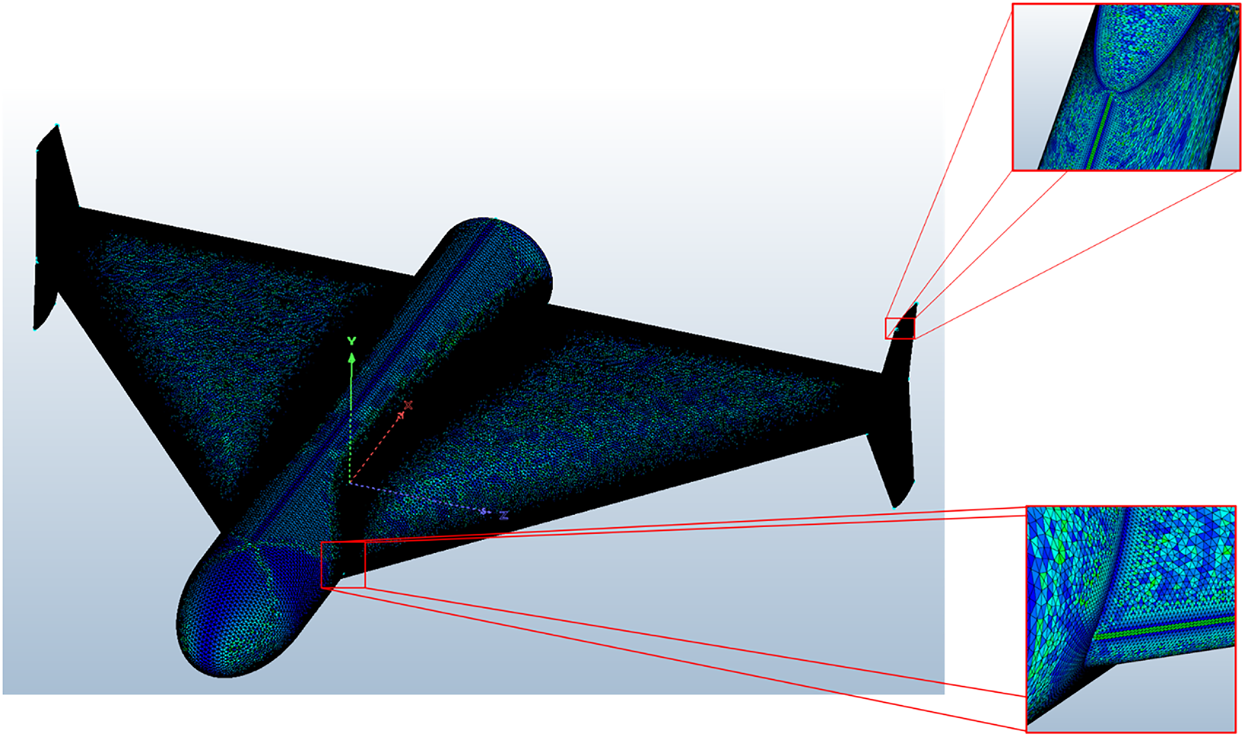
The UAV geometry is discretised using Fidelity Pointwise. The chosen meshing approach utilises tetrahedral cells and leverages tetrahedral extrusions (T-Rex) for the generation of high-quality boundary layers and the overall volume mesh. This strategy minimises the potential for collapsing of the boundary layers during the simulation process. The leading and trailing edges of the model are refined to capture the curvature of the model as seen from the surface mesh shown in Fig. 1.
Surface mesh for the CFD.

The first-cell height of the boundary layer was selected such that the non-dimensional wall distance
 ${y^ + }$
remained below 1 across the entire UAV surface. This ensured accurate resolution of the viscous sublayer and permitted reliable prediction of skin-friction drag, stall onset and separation behaviour. The computational domain was constructed with a characteristic extent of approximately
 $20L$
, where
 $L$
denotes the reference length of the UAV, in order to minimise blockage effects and accurately represent far-field flow conditions.
4.3 Mesh independence study and validation
A mesh independence study was conducted to determine an appropriate grid resolution. Simulations were performed at angles of attack of
 ${0^ \circ }$
,
 ${5^ \circ }$
and
 ${10^ \circ }$
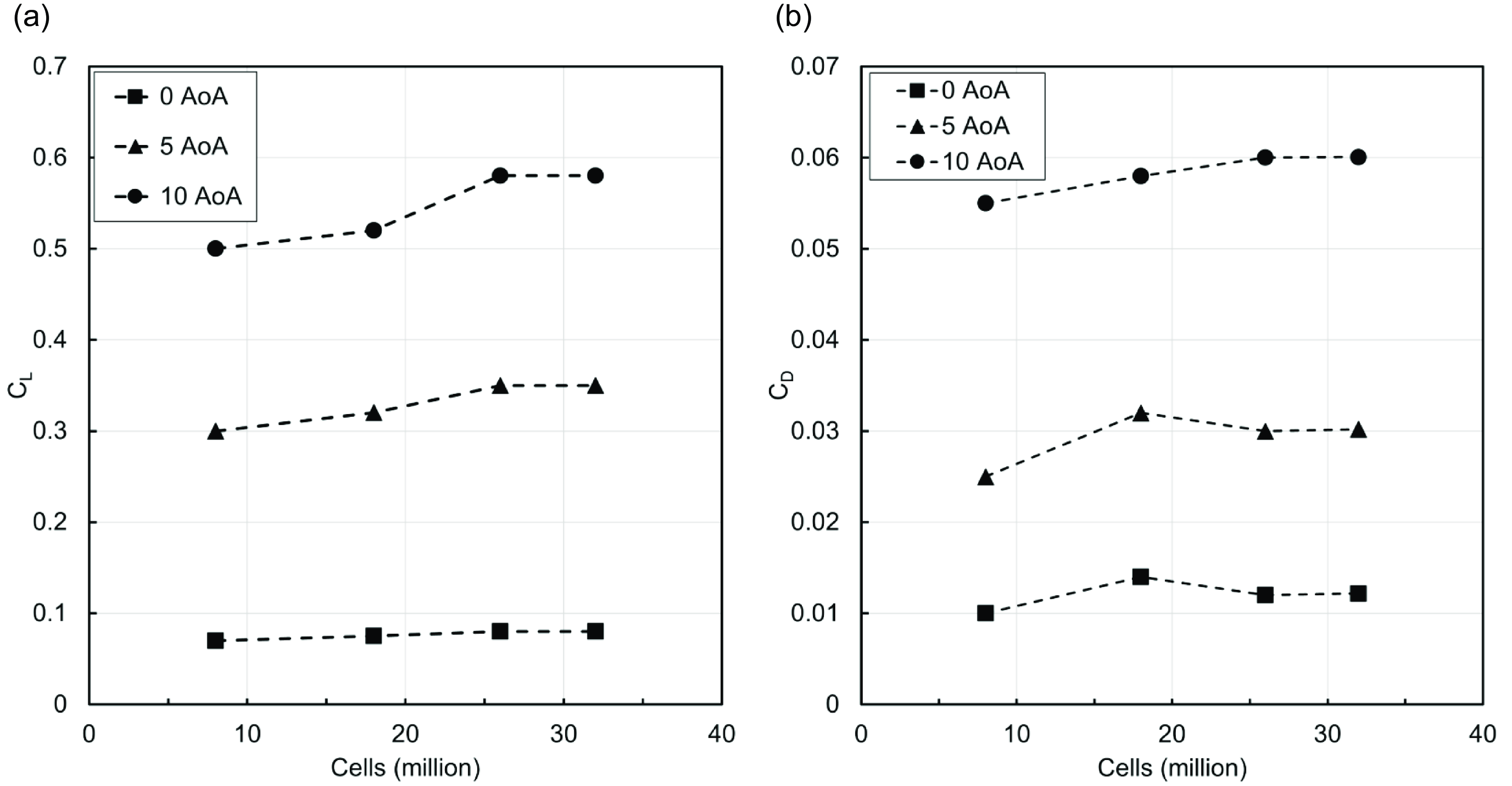
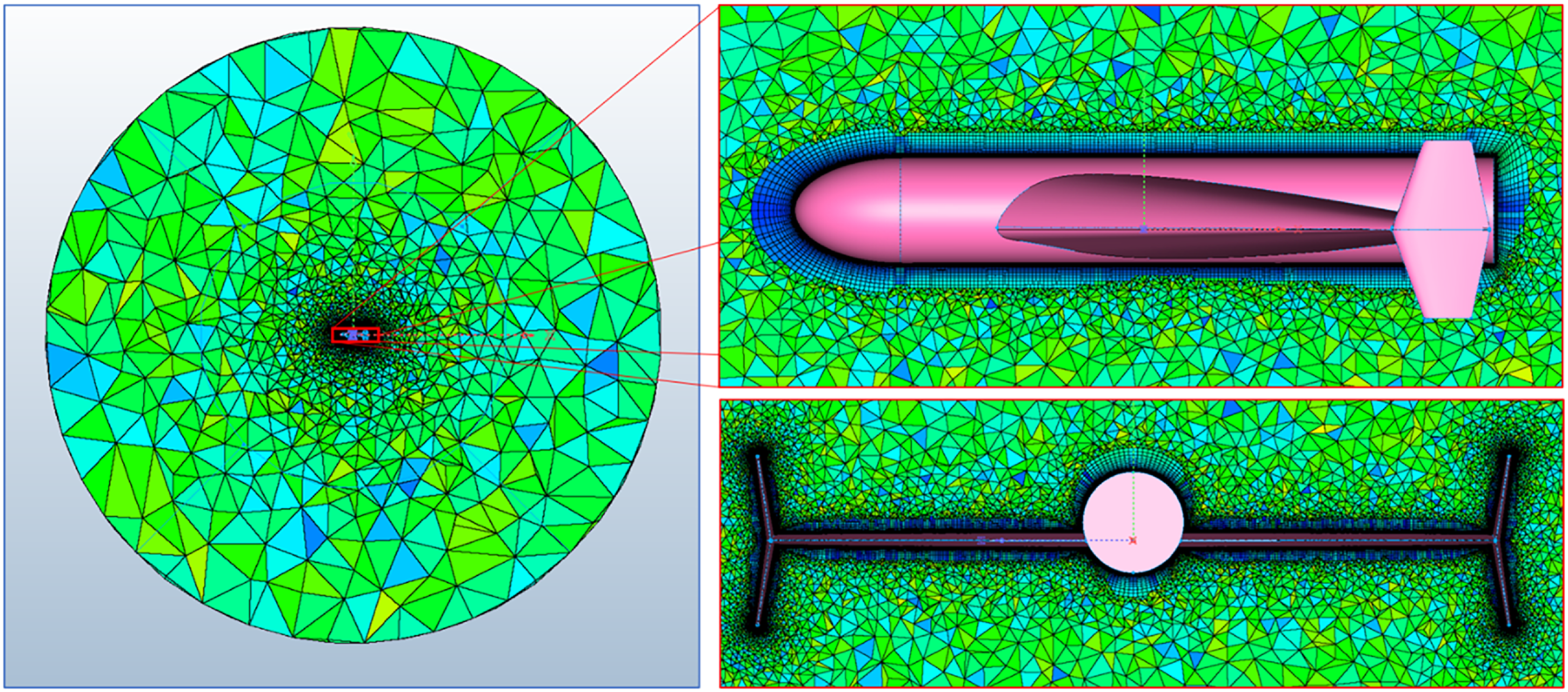
using a sequence of progressively refined meshes. The variation in aerodynamic coefficients diminished with increasing cell count, as illustrated in Fig. 2. A mesh containing approximately 26 million cells was selected as the optimal configuration, as further refinement produced negligible changes in both the lift coefficient
 ${C_L}$
and drag coefficient
 ${C_D}$
across all evaluated angles of attack. The final volume mesh is shown in Fig. 3.
Mesh independence study for variation of
 ${C_L}$
and
 ${C_D}$
with angle-of-attack. (a) Variation of CL with mesh cells. (b) Variation of CD with mesh cells.

Volume mesh for the CFD.

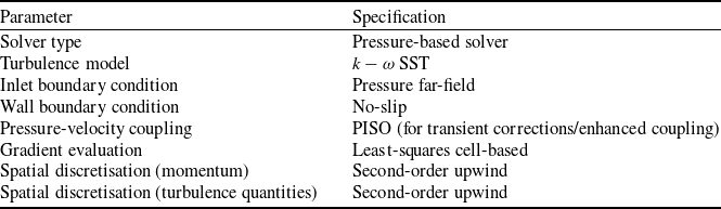
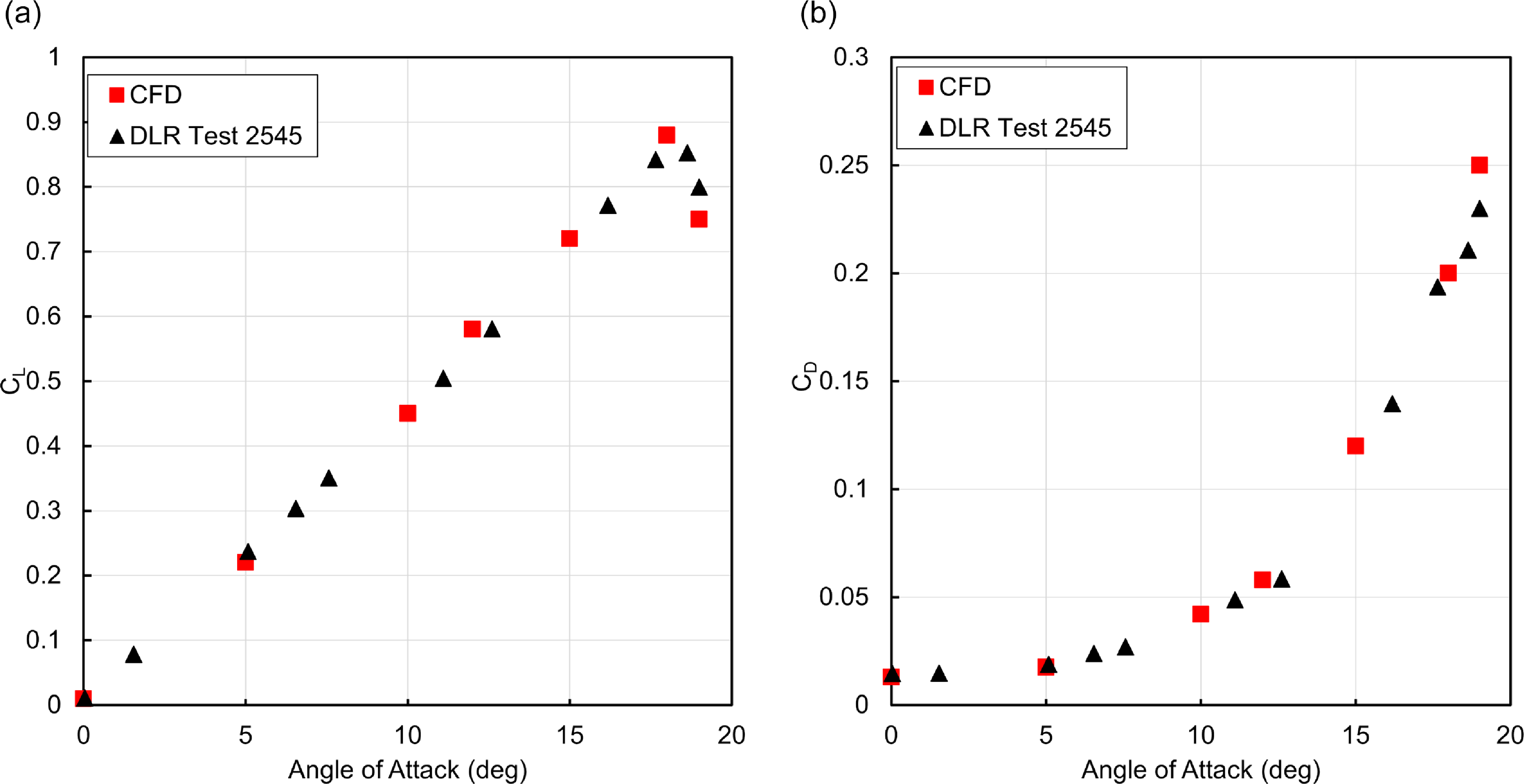
Based on the selected mesh configuration, a validation study was carried out using a generic tailless UAV model. The aerodynamic coefficients obtained from the CFD simulations were compared with the experimental data reported in Ref. [Reference Ghoreyshi, Jirasek, Cummings, Da Ronch and Young22]. The geometry was reconstructed and meshed using the same grid generation strategy and mesh parameters established during the mesh independence study. The simulation was performed using OpenFOAM v2112 and the computational setup used is summarised in Table 2. The comparison results, presented in Fig. 4, demonstrate close agreement between the numerical and experimental data, thereby confirming the reliability of the adopted meshing approach and solver settings.
Summary of computational setup

Mesh and computational setup validation for generic tailless UAV with experimentaldata. (a) Validation of CL. (b) Validation of CD.

5.0 Computational setup for RCS analysis
RCS quantifies the detectability of an object by radar and is defined as the surface area intercepting that amount of incoming radar wave which, when scattered isotropically, produces an echo at the radar equal to the scattering target. In term of aircrafts, the smaller the RCS, the stealthier the design making it less detectable on the radar. RCS is not only dependent on size of the object but also on its geometric structure, material, frequency and polarisation of the incoming radar wave. For simple electrically small geometries, RCS can often be estimated using mathematical formula or closed loop solutions. However, for electrically large or complex-shaped objects, accurate RCS analysis requires full-wave electromagnetic simulations (MoM, IE) that account for diffraction, multiple scattering and material properties. As the geometric complexity increases, so does the simulation time and computational resource required to perform the analysis particularly, due to finer meshing requirements and the need to capture intricate field interactions. Aircraft with a smaller RCS corresponds to a stealthier design, less observable to the radar thus smaller detection range [Reference Bilal, Hamza, Taj and Salamat23]. RCS is basically the projected area of any object to the radar waves. RCS is measured in dBsm or m
 ${{\rm{\;}}^2}$
.
The mathematical formulation for RCS [Reference Hoseini, Abdolali, Fallah and Amir-Hosseini24] is outlined as:
 \begin{align}\sigma = 4\pi \mathop {{\rm{lim}}}\limits_{r \to \infty } {r^2}\frac{{{E_s}^2}}{{{E_i}^2}}\end{align}
Here
 $\sigma $
is RCS.
 ${E_i}$
is the incident electric field whereas
 ${E_s}$
is the scattered electric field whose strength is dependent on the distance
 $r$
. For our analysis, we take monostatic RCS which means both the transmitter and receiver are placed in the same place (contrary to bistatic).
For simulating the RCS of an object, there are many CEM algorithms which make use of the integral or differential form of Maxwell equations. Commonly used algorithms are physical optics/geometric optics, method of moment (MoM), multilevel fast multipole method (MLFMM) and shooting and bouncing rays (SBR) [Reference Bilal, Hamza, Taj and Salamat25]. PO employs light diffraction for calculating RCS. PO is fast but is less accurate due to its shortcoming in capturing the effect of edge diffraction and multibounce waves on object’s surface. MoM and MLFMM are high-fidelity methods with greater accuracy but require high computational resource and time. SBR resolves the shortcoming of these methodologies by catering for edge diffraction, surface creeping waves and calculating multi bounce effect of the incident waves. This results in a fast and comparatively accurate result.
SBR uses optical ray tubes for simulating incident (EM) waves. The traveling rays obeys the principle of geometric optics which under Fermat’s principle states that a ray travels on a straight path/line. The path of propagation is written as:
 \begin{align}r\left( {x,y,z} \right) = {r_o}\left( {{x_o},{y_o},{z_o}} \right) + s( {{s_x},{s_y},{s_z}} )t\end{align}
where
 ${r_0}$
represents the initial starting point,
 $s$
represents the direction of propagation and
 $t$
is the time taken on the path being followed by the ray. This traveling ray will reflect or refract from the target when it is incident of the surface. The ray’s direction (reflection/reflection) can be found using Snell’s law. Moreover, the scattered waves generated by reflection from the target surface employs PO principle on ray tubes for integration of far field. The equation for scattered field from target’s surface, using the Stratton-Chu formula, can be written as:
 \begin{align}{E_s} = {{ - jk{Z_o}{e^{ - jkr}}} \over {4\pi r}}\mathop \int\!\!\!\int \limits_s s \times \left( {s \times J} \right){e^{\,jkr\left( {i - s} \right)}}dS\end{align}
In the equation,
 $k$
is the wave number.
 ${Z_0}$
is the intrinsic impedance of the target space. The vector
 $s$
is the directional unit vector of scattered wave and
 $i$
is the scattered wave directional vector. The illuminated portion of the target is represented by
 $S$
.
6.0 Design of experiments
To efficiently and systematically explore the design space of the coupled aerodynamic – RCS optimisation problem, a design of experiments (DoE) strategy was adopted. DoE is a structured methodology that enables the extraction of maximum information from a minimal number of simulations or physical tests [Reference Ashwin Renganathan, Maulik and Ahuja26]. It achieves this by strategically varying the design variables (input factors) to evaluate their influence on the response variables of interest, while relying on statistical principles to ensure robustness and reproducibility of the results. In the present work, the DoE was specifically implemented using the central composite design (CCD), a well-established approach for constructing second-order (quadratic) response surfaces that can capture curvature effects in the objective space.
The CCD combines three sets of design points: (1) factorial points, which explore combinations of high and low levels for each factor; (2) axial (star) points, positioned at a distance
 $\alpha $
from the design centre to capture curvature effects; and (3) centre points, located at the midpoint of all factors to provide a baseline and improve the estimation of experimental error.
In a CCD, the factorial portion defines the main interaction effects, the axial points estimate the curvature of the response surface, and the centre points ensure statistical stability. The distance
 $\alpha $
from the design centre to the star points depends on the number of factors
 $k$
and the type of CCD selected (circumscribed, inscribed or face-centred). In general, a CCD contains twice as many axial points as there are factors in the design.
For the present study, a face-centred central composite design (FCCD) was selected due to its balanced trade-off between exploration range and computational efficiency. Compared to a circumscribed CCD, the FCCD requires fewer simulation runs while still covering the full range of factor levels. Unlike the inscribed CCD, which reduces the design space to fit within the factorial limits, the FCCD allows full exploration of the original parameter boundaries. In FCCD, each factor is evaluated at three levels: its minimum, baseline (centre) and maximum. The total number of experiments
 $N$
for an FCCD is given by:
 \begin{align}N = {2^k} + 2k + 1\end{align}
where
 $k$
represents the number of design variables. The limits of each variable were set according to aerodynamic feasibility and RCS constraints, ensuring that the generated designs remain practical and physically realisable.
Point distribution in the central composite design for four variables

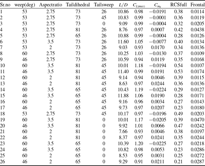
In the FCCD employed for this study, a total of 25 design points were generated for the four selected design variables (Table 3). These include
 ${2^k} = 16$
factorial points that represent all combinations of the variables at their upper
 $\left( { + 1} \right)$
and lower
 $\left( { - 1} \right)$
coded levels, and
 $2k = 8$
axial (star) points, where one variable is set to an extended level
 $\left( { \pm \alpha } \right)$
while the remaining variables are held at their mean
 $\left( 0 \right)$
level to capture curvature effects. Additionally, a single centre point
 $\left( {0,0,0,0} \right)$
is included to assess repeatability and detect non-linearity. Therefore, the CCD matrix consists of 25 unique geometrical configurations. When the baseline configuration is also included for reference, the total number of geometries considered in this work becomes 26.
Once the DoE matrix was established, response surface methodology (RSM) was employed to construct an analytical surrogate model that relates the input factors to the output responses. RSM approximates the true response surface using a polynomial equation, enabling rapid evaluation during optimisation. For
 $n$
factors, the general second-order RSM model is expressed as:
 \begin{align}Y = {a_0} + \mathop \sum \limits_{i = 1}^n {a_i}{k_i} + \mathop \sum \limits_{i = 1}^n \mathop \sum \limits_{j = i + 1}^n {a_{ij}}{k_i}{k_j} + \mathop \sum \limits_{i = 1}^n {a_{ii}}x_i^2\end{align}
where
 $Y$
is the predicted response,
 ${k_i}$
are the coded design variables,
 ${a_0}$
is the intercept,
 ${a_i}$
are the linear coefficients,
 ${a_{ij}}$
represent interaction effects between variables, and
 ${a_{ii}}$
capture the quadratic curvature terms.
The combined use of DoE (via FCCD) and RSM enables the construction of an accurate, computationally inexpensive surrogate model that captures the complex, nonlinear interactions between aerodynamic and RCS performance metrics. This surrogate model serves as the foundation for the subsequent gradient-based optimisation stage, allowing rapid identification of optimal design parameters while minimising the number of high-fidelity simulations required.
Table 4 presents the DoE matrix developed for this study, consisting of 26 distinct configurations generated by CCD approach and varying the sweep angle, aspect ratio, tail dihedral and tail sweep angle. For each case, a parametric computer-aided design (CAD) model was created and subsequently analysed using both CFD and RCS simulations. The corresponding aerodynamic and electromagnetic performance metrics are also reported in Table 4. These simulation results form the basis for constructing the quadratic RSE, which serve as surrogate models to enable efficient evaluation of the objective function and constraints during the optimisation process.
Response surface results

7.0 Optimisation scheme
The optimisation framework employs a constrained interior-point algorithm with a Broyden-Fletcher-Goldfarb-Shanno (BFGS) quasi-Newton Hessian approximation, targeting the (barrier) Karush–Kuhn–Tucker (KKT) conditions [Reference Frédéric Bonnans, Charles Gilbert, Lemaréchal and Sagastizábal27–Reference Wächter and Biegler29]. An in-house optimisation code was developed based on this approach.
Multiple design goals are combined into a single differentiable scalar objective
 $f\left( x \right)$
subject to
 $c\left( x \right) = 0$
(equality) and
 $g\left( x \right) \le 0$
(inequality) constraints:
 \begin{align}f\left( x \right){\rm{\;\;}} = {\rm{\;\;}} - \frac{{{C_{{L_{{\rm{max}}}}}}\left( x \right)}}{{C_{{L_{{\rm{max}}}}}^{\left( {{\rm{max}}} \right)}}}{\rm{\;\;}} + {\rm{\;\;}}\frac{{{\rm{RC}}{{\rm{S}}_{{\rm{overall}}}}\left( x \right)}}{{{\rm{RCS}}_{{\rm{overall}}}^{\left( {{\rm{max}}} \right)}}}{\rm{\;\;}} + {\rm{\;\;}}\frac{{{\rm{RC}}{{\rm{S}}_{{\rm{frontal}}}}\left( x \right)}}{{{\rm{RCS}}_{{\rm{frontal}}}^{\left( {{\rm{max}}} \right)}}}.\end{align}
High-fidelity metrics are emulated with quadratic RSEs, allowing analytical gradients.
Inequalities are written in slack form
 $g\left( x \right) + s = 0$
with
 $s \gt 0$
. For a barrier parameter
 $\tau \gt 0$
, the barrier-augmented Lagrangian is:
 \begin{align}{\mathcal{L}_\tau }\left( {x,s,\lambda ,\nu } \right){\rm{\;}} = {\rm{\;}}f\left( x \right) + {\lambda ^{\rm T}}c\left( x \right) + {\nu ^{\rm T}}\left( {g\left( x \right) + s} \right) - \tau {\rm{\;}}\mathop \sum \limits_i {\rm{ln}}{s_i}\end{align}
The perturbed KKT first-order optimality conditions are:
 \begin{align} \displaystyle{{\nabla _x}{\mathcal{L}_\tau }\left( {x,s,\lambda ,\nu } \right)} {} &= 0,\nonumber\\[5pt] \displaystyle {c\left( x \right)} {} &= 0,\nonumber\\[5pt] \displaystyle {g\left( x \right) + s} {} &= 0,\\[5pt] \displaystyle {S\nu } {} &= \tau {\bf{e}},{\rm{\;\;\;\;}}s \gt 0,\;\;\nu \gt 0, \nonumber \end{align}
where
 $S = diag\left( s \right)$
,
 ${\bf{e}}$
is the vector of ones, and
 $\left( {\lambda ,\nu } \right)$
are multipliers.
For a given
 $\tau $
, the primal–dual Newton step
 $\left( {{\rm{\Delta }}x,{\rm{\Delta }}s,{\rm{\Delta }}\lambda ,{\rm{\Delta }}\nu } \right)$
is found by solving the linearisation of (15):
 \begin{align}\begin{bmatrix}H\;\;\;\; & J_c^\top\;\;\;\; & J_g^\top\;\;\;\; & 0 \\J_c\;\;\;\; & 0\;\;\;\; & 0\;\;\;\; & 0 \\J_g\;\;\;\; & 0\;\;\;\; & 0\;\;\;\; & I \\0\;\;\;\; & 0\;\;\;\; & S\;\;\;\; & V\end{bmatrix}\begin{bmatrix}\Delta x \\ \Delta \lambda \\ \Delta \nu \\ \Delta s\end{bmatrix}=-\begin{bmatrix}\nabla_x \mathcal{L}_\tau \\ c(x) \\ g(x)+s \\ S\nu - \tau \mathbf{e}\end{bmatrix},\end{align}
with
 ${J_c} = \nabla c\left( x \right)$
,
 ${J_g} = \nabla g\left( x \right)$
,
 $V = diag\left( \nu \right)$
, and
 $H$
as the Hessian of the Lagrangian.
The Hessian
 $H$
is approximated using the BFGS update:
 \begin{align}{H_{k + 1}}{\rm{\;\;}} = {\rm{\;\;}}{H_k}{\rm{\;\;}} + {\rm{\;\;}}\frac{{{y_k}y_k^{\rm T}}}{{y_k^{\rm T}{s_k}}}{\rm{\;\;}} - {\rm{\;\;}}\frac{{{H_k}{s_k}s_k^{\rm T}{H_k}}}{{s_k^{\rm T}{H_k}{s_k}}},\end{align}
where
 ${s_k} = {x_{k + 1}} - {x_k}$
and
 ${y_k} = {\nabla _x}{\mathcal{L}_\tau }\left( {{x_{k + 1}}} \right) - {\nabla _x}{\mathcal{L}_\tau }\left( {{x_k}} \right)$
.
A backtracking line search finds
 $\alpha \in \left( {0,1} \right]$
for the primal-dual step. This step is constrained by a fraction-to-the-boundary rule and accepted based on sufficient decrease of a barrier merit function [Reference Byrd, Hribar and Nocedal28].
8.0 Results and discussion
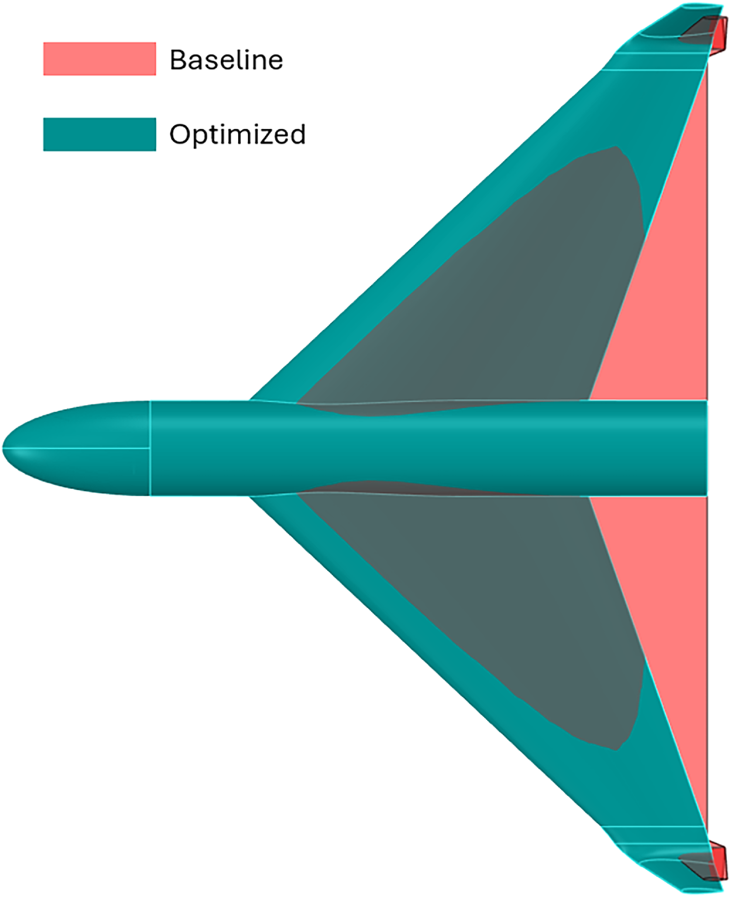
Following the iterative optimisation, a global minimum is identified, which remains consistent across different initial conditions. The parameters corresponding to this global minimum are utilised to generate a new CAD model. The optimised CAD model obtained is shown in Fig. 5.
Baseline vs optimised model.

8.1 Aerodynamic analysis
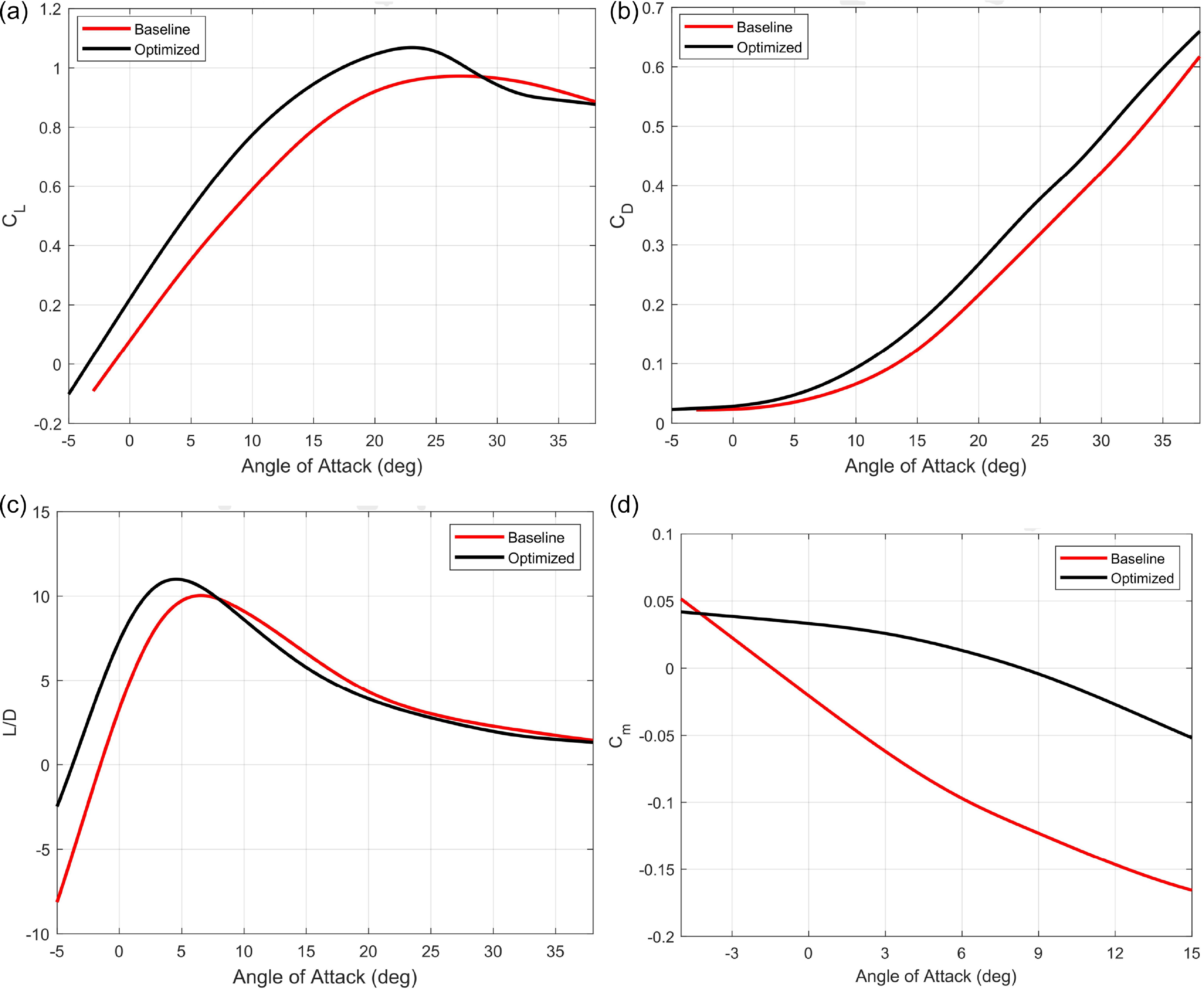
The optimised CAD model is subjected to aerodynamic analysis through CFD. The results, as depicted in Fig. 6(a), reveal a significant improvement in the lift coefficient (
 ${C_L}$
) compared to the baseline model. It is noteworthy that the optimised model exhibits higher lift, aligning with the objective of the optimisation process.
Comparison of aerodynamic coefficients with baseline model. (a) Lift coefficient comparison. (b) Drag coefficient comparison. (c) Aerodynamic efficiency comparison. (d) Pitch moment coefficient comparison.

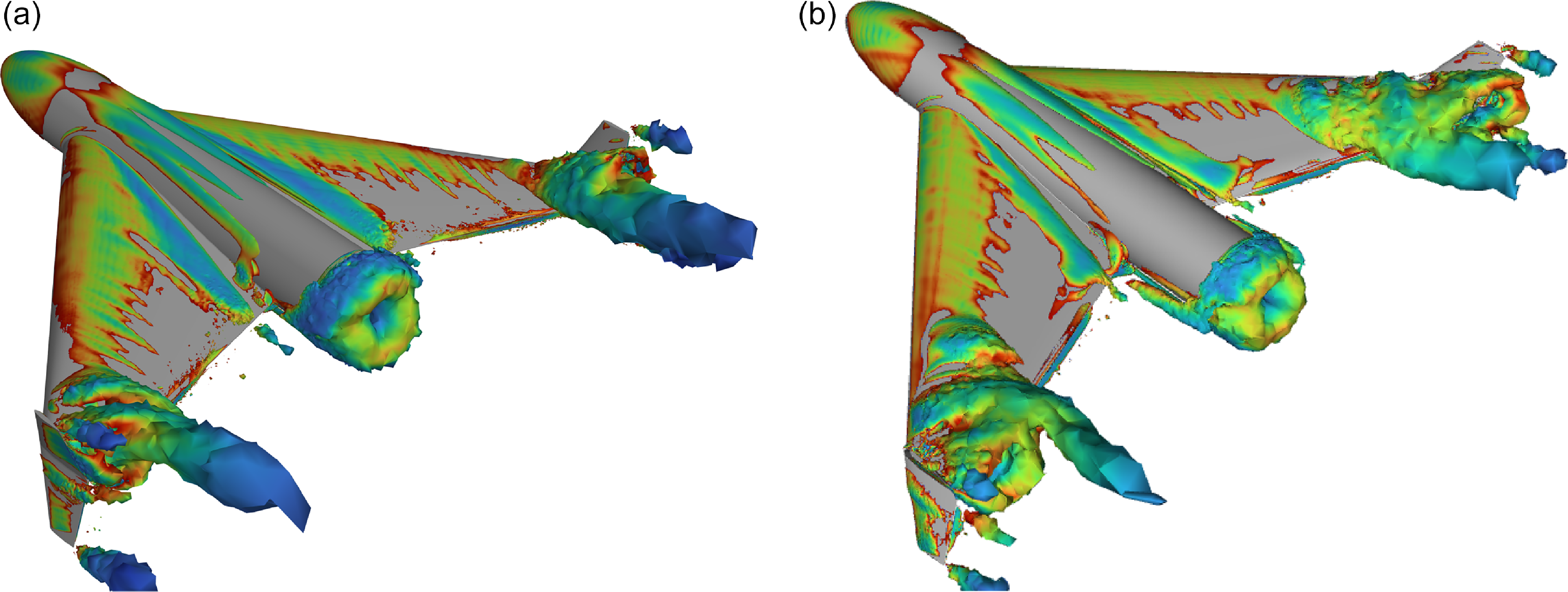
Comparison of vortices generated on baseline vs optimised model. (a) Vortices on optimised UAV. (b) Vortices on baseline UAV.

However, the overall drag was not explicitly considered during the optimisation, resulting in increased drag for the optimised model as observed in Fig. 6(b). This trade-off between lift and drag underscores the importance of considering both factors in future optimisation iterations. Furthermore, the optimised model also meets all the design constraints defined in the optimiser.
One of the design constraints stipulated that the L/D should be greater than 10. As shown in Fig. 6(c), the optimised model successfully meets this constraint, demonstrating its improved aerodynamic performance.
Another crucial constraint was ensuring a positive pitch moment coefficient (
 ${C_{m0}}$
) for stability. Figure 6(d) illustrates not only the fulfilUAVent of the positive
 ${C_{m0}}$
constraint but also a more negative slope of the pitch moment curve (
 ${C_{ma}}$
), indicating improved longitudinal stability for the optimised model.
The results demonstrate the success of the optimisation process in enhancing the overall lift coefficient while meeting critical design constraints as shown in Fig. 6(a). The trade-off between lift and drag is acknowledged, but the aerodynamic performance of an aircraft is directly related to the aerodynamic efficiency i.e. L/D ratio which has increased overall. The positive impact on longitudinal stability further reinforces the improved performance of the optimised model.
Structurally the aspect ratio has been increased by 25% which has an effect on induced drag by reducing it which is shown in the L/D values of the UAV. Wing sweep has been reduced by 4 degree, which affects both lift and drag generation. The decrease in sweep angle improves the low-speed performance of the UAV as well increasing the overall maximum lift coefficient. However, the increase in sweep angle also increases the overall drag. However, the aerodynamic efficiency of the UAV depends on the L/D ratio and is not a function of drag alone. Therefore, the overall aerodynamic performance of the UAV has improved as shown in Fig. 6(b).
In addition, the optimised model results in smaller vortices generated during the cruise condition near the wing tip as opposed to the baseline model as seen in Fig. 7. The vortices generated on the baseline model are more violent in nature and travel further downstream than the optimised model. This shows that the optimised UAV has better aerodynnamic performance than the baseline model.
8.2 RCS analysis
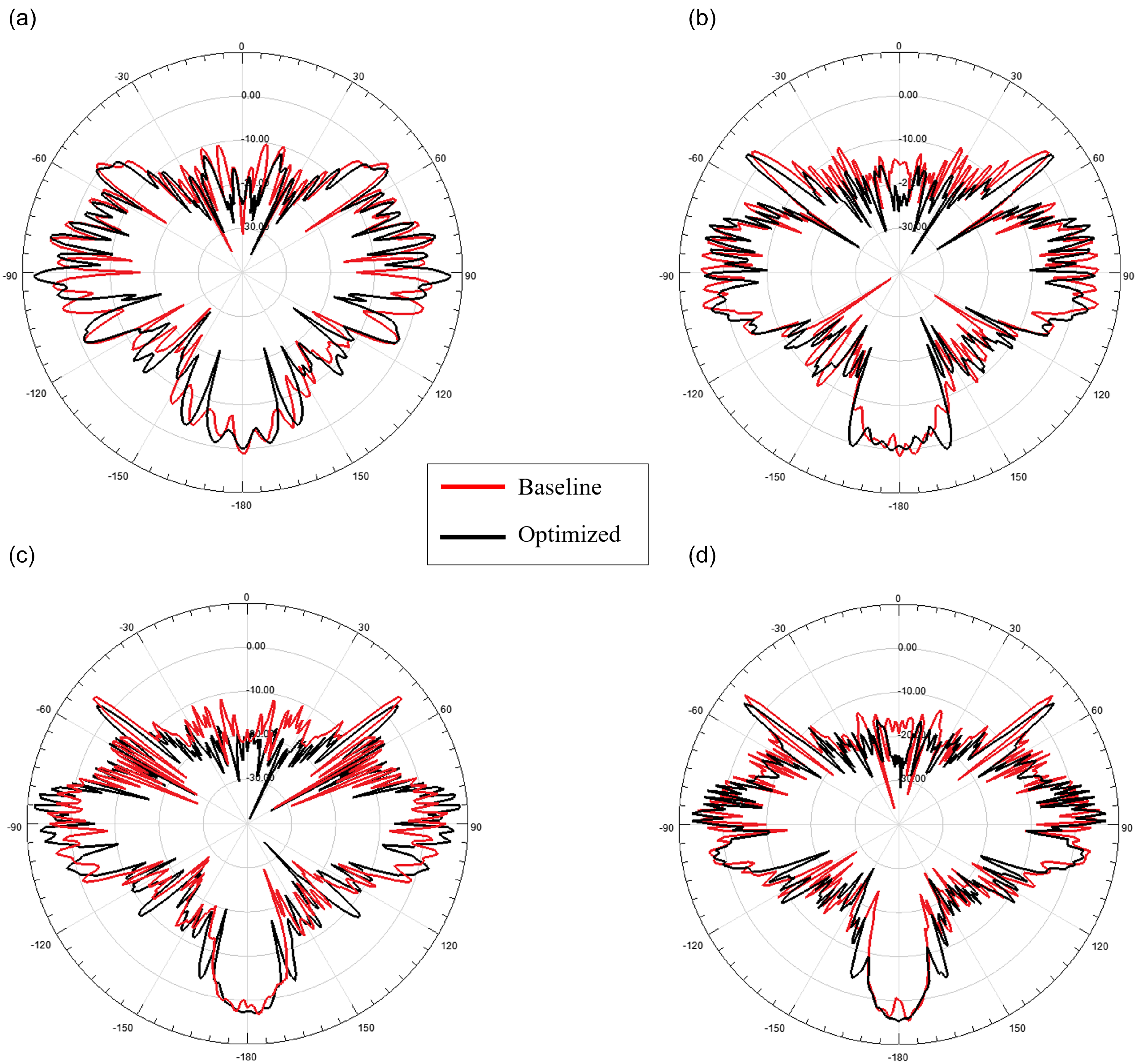
The monostatic RCS of the baseline and optimised geometry is computed using SBR technique at four frequencies: 1GHz, 1.5GHz, 2GHz, 2.5GHz in horizontal (HH) polarisation. These are commonly used frequencies in most of the modern ground based long range search and track radars. For simulation, the material of the model is taken as perfect electric conductor (PEC). The azimuth angle varies from
 ${0^ \circ }$
to
 ${360^ \circ }$
with
 ${1^ \circ }$
step size while the elevation angle is fixed at
 ${0^ \circ }$
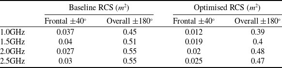
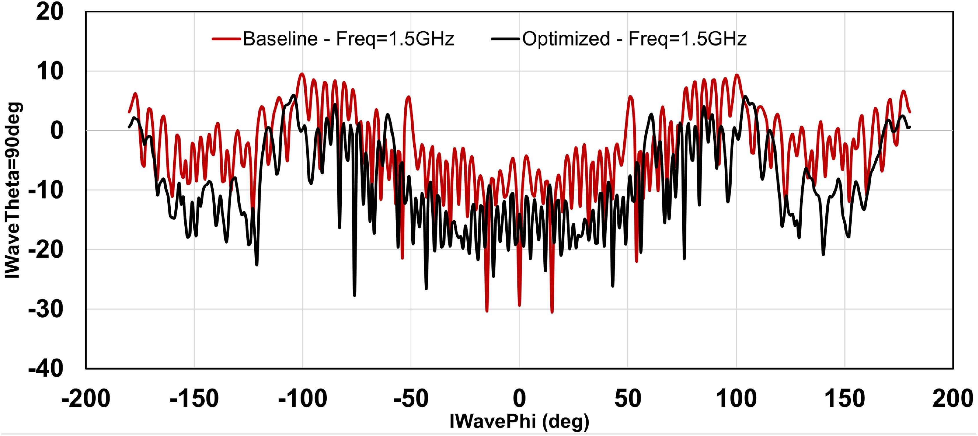
(nose front) for illuminating the model with plane waves. The corresponding RCS value for each frequency for both baseline and optimised model is outlined in Table 5 and their polar plots are shown in Fig. 8.
RCS of baseline and optimised model

Polar plots of baseline and optimised model.

From Table 5 it can be seen that the RCS value in the overall and frontal aspect for the optimised design is considerably smaller. This is attributed to the optimised design of wing blending, aspect ratio and wing sweep that has mitigated wave reflections in critical areas hence reducing RCS. A gradual increase in RCS is seen with increase in frequency. The RCS are measured in overall (
 $ \pm {180^ \circ }$
) and frontal (
 $ \pm {40^ \circ }$
) aspect. Moreover, the polar plot comparison of baseline and optimised geometry highlights the reduction in key reflection areas.
The comparison of RCS values of baseline and optimised design is shown in Fig. 9. The mean RCS of overall aspect of the baseline design is 1.30
 ${m^2}$
and frontal aspect 0.35
 ${m^2}$
.
The overall and frontal RCS of optimised geometry is 0.45
 ${m^2}$
and 0.045
 ${m^2},$
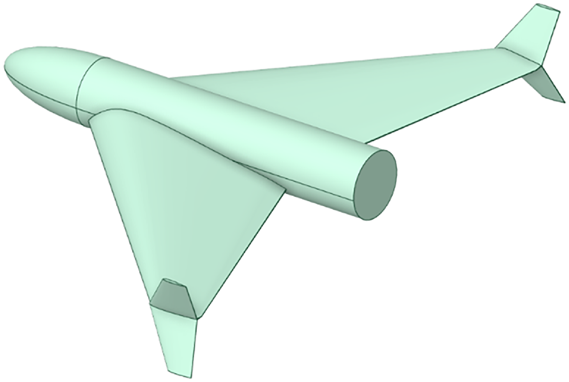
respectively. This is a considerable improvement in the RCS reduction as not only the radar signature has been mitigated but the aerodynamic performance has been improved with reduction in interference drag. The final optimized geometry is shown in Fig. 10 and is used for experimental validation.
Comparison of base geometry and optimised geometry.

Final CAD model.

9.0 Experimental validation of RCS
9.1 Model design, fabrication and testing
The final optimised design is used to generate a small-scale model for experimental RCS testing. The full-scale model has a total length of 1 m with a wingspan of 1.2 m. For testing purposes, the model is scaled down to 1:6 to fit the size of the anechoic chamber. To ensure that the effects observed are equivalent to those of testing a full-size model, the sweep frequency is also scaled up by the same factor. Material properties in this context remain unaffected by the scaling factor. The subsequent scaled frequencies are 6 GHz, 9 GHz, 12 GHz and 15 GHz (which correspond to 1 GHz, 1.5 GHz, 2 GHz and 2.5 GHz in actuality).
The model is fabricated using 3D printing technique. The base material for synthesising material is based on PETG resin. The resin is grey PLA and has a density of 1.27
 $g/c{m^3}$
. The 3D printing is performed using an Elegoo Neptune 4 3D printer, which has built volume of 225 × 225 × 265
 $m{m^3}$
with a filament diameter of 0.4mm. After model synthesis, the outer surface is smoothened by carefully buffing the rough corners of the material without effecting the surface texture. The 3D printed model is an exact match to the original platform in CAD model. For conductivity, the surface of the model is coated with CHO-SHIELD 4900 conductive paint which imitates the exact conductivity and dielectric properties of the PEC material.
The RCS test chamber has a volume of 2m
 $ \times {\rm{\;}}$
2m
 $ \times {\rm{\;}}$
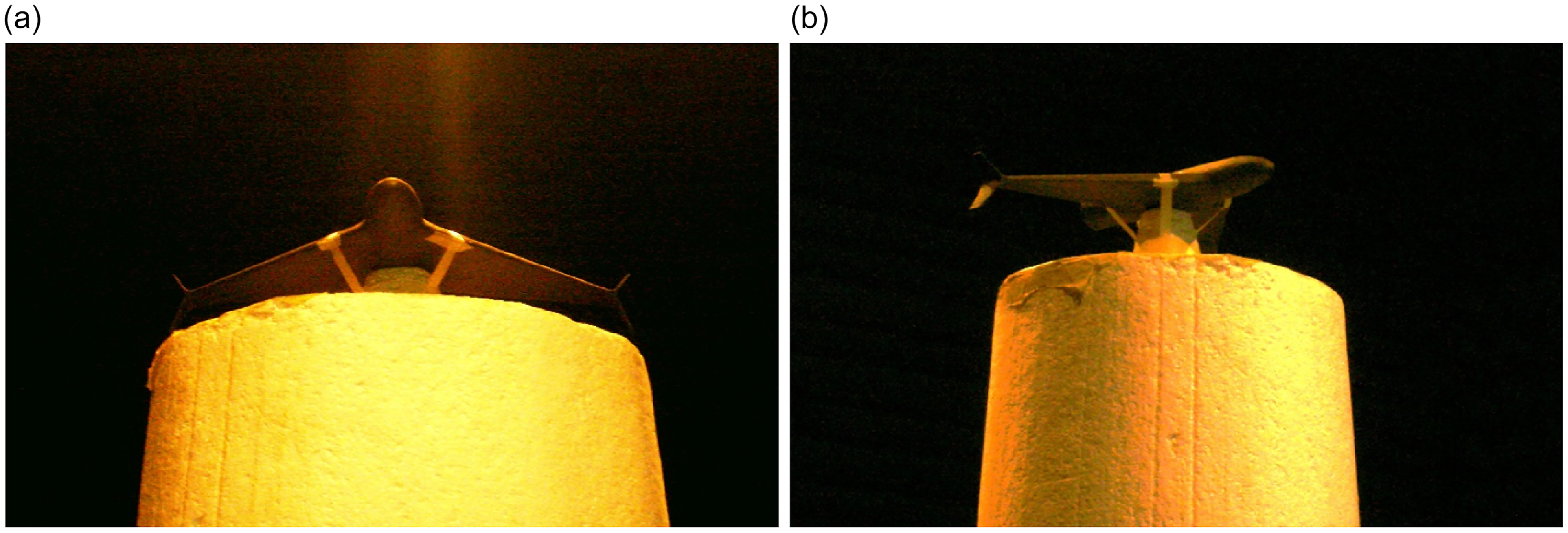
4m. The experimental setup for RCS measurement is shown in Fig. 11(b).
The RCS chamber is a dual reflector setup with the main reflector antenna spanning at a length of 15ft, width of 8ft and height of 6ft. Max frequency range of the chamber is 40GHz. The chamber walls are covered with RF absorbers to minimise the overall noise floor and external interference. The elevation and plane of the reflector antenna can vary but in our test case it is fixed at
 $ \pm {0^ \circ }$
.
9.2 Results and discussion
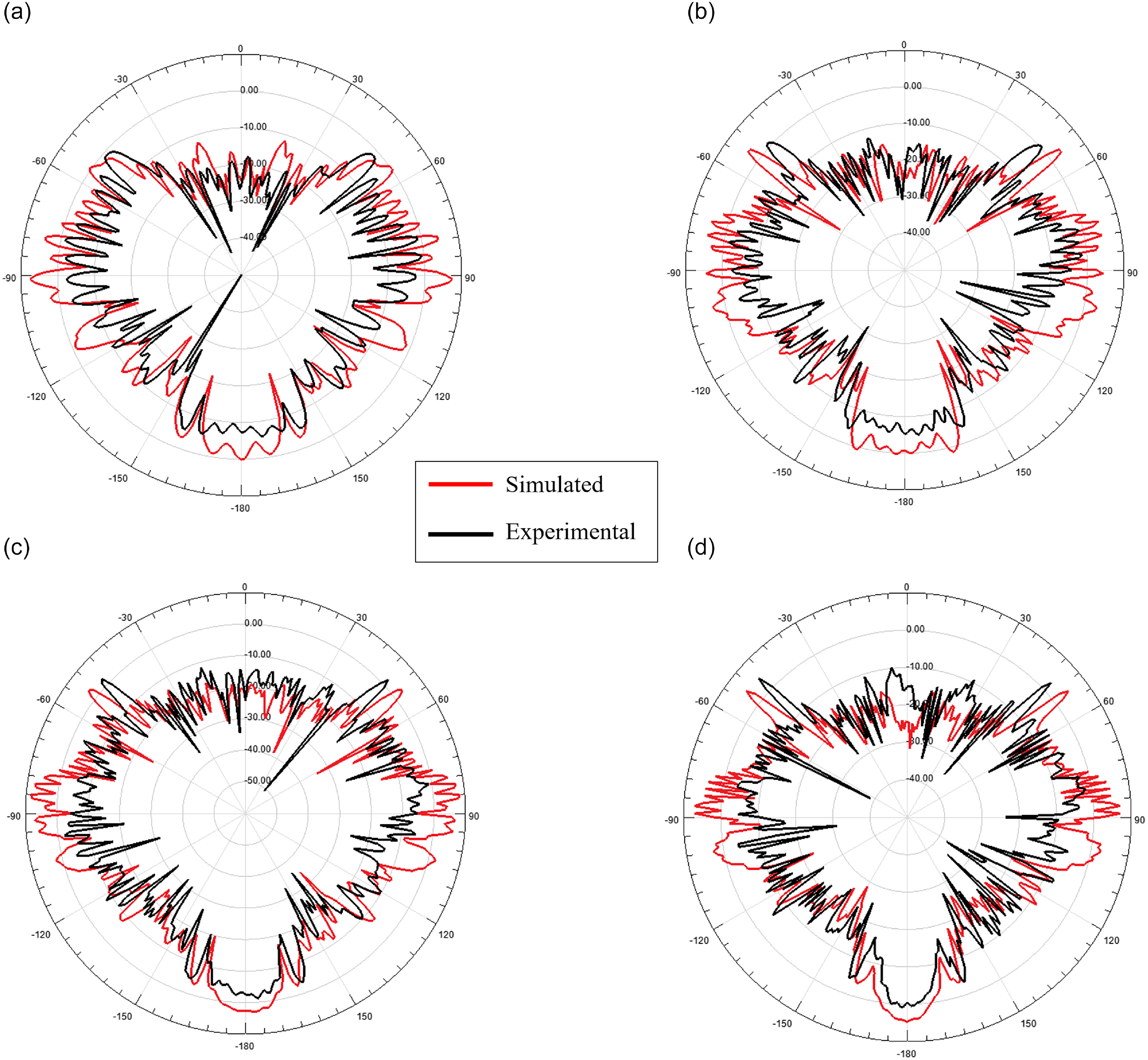
The simulated and test measurement results are compared. As can be observed, the superimposed polar plots for each test frequency is outlined in Fig. 12 The azimuth angle is varied while the elevation is fixed at
 $\phi = {0^ \circ }$
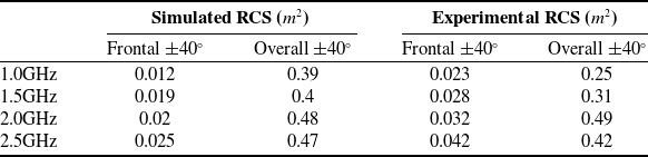
, which corresponds to the nose of the platform. The comparison shows the accuracy for the test measurement setup for calculating RCS. The slight deviation is attributed to less than ideal surface variation and paint application.
The comparison table for the simulated and measured RCS values of the platform against each frequency is outlined in Table 6. The results are in close agreement, validating the simulation results for the platform.
RCS validation of optimised model

10.0 Conclusion
This study presented a comprehensive approach to the aerodynamic and RCS optimisation of a UAV using a surrogate model-based optimisation algorithm. The optimisation process resulted in a 12% increase in the overall lift coefficient (
 ${C_L}$
) and a 30% reduction in both the overall and frontal RCS. The improvements in aerodynamic performance and stealth capabilities were achieved while maintaining critical constraints on the lift-to-drag ratio (L/D) and pitch moment coefficient (
 $C_{m0}$
).
The use of high-fidelity simulations and experimental testing validated the accuracy and practical applicability of the optimised design. The iterative approach and consideration of multiple initial conditions ensured the robustness of the optimisation process, addressing potential local minima issues and enhancing the reliability of the results.
Overall, this study demonstrated the effectiveness of a multi-objective optimisation scheme in enhancing the Aero-RCS performance of UAVs. The findings provide valuable insights for future UAV design and optimisation efforts, emphasising the importance of a balanced approach to aerodynamic efficiency and stealth capabilities.
Future efforts will involve experimental aerodynamic verification of the optimised UAV design using wind tunnel testing. A scaled model will be built and fitted with force and moment sensors to obtain aerodynamic coefficients over a range of angles of attack and sideslip angles. The experimental data will be compared with computational analysis to evaluate accuracy and tune the aerodynamic model.
Anechoic chamber for RCS testing. (a) RCS chamber front. (b) RCS chamber side.

Polar plots of simulated and experimental model.

Funding statement
No external funding was required for this research.
Author contributions
AIA and SMH conceived the idea. AIA performed the CAD modelling, CFD analysis and optimisation. SMH was responsible for RCS analysis and experimental validation. IAS and MA supervised the work and helped edit the paper.
Conflict of interests
Authors state no conflict of interest.