The amount and explanation of catch-up growth in the heights of teenage slaves are outstanding questions in the history of American slavery. In 1986 Richard Steckel analyzed shipping manifests and reported that slaves were among the smallest children ever measured but as adults were nearly as tall or taller than many European nobility (Steckel Reference Steckel1986).Footnote 1 This upward movement through the percentiles was equivalent to catch-up (or compensatory) growth of approximately four inches relative to modern height standards. This remarkable catch-up is not unprecedented but is very unusual relative to current and historical patterns of physical growth.
Interpreting the extensive catch-up growth as evidence for selective feeding on the part of owners by age of the slave, Steckel's finding has enormous implications for how economists view plantation management and the treatment of slaves, particularly children. Simply put, the height evidence shows that slave children bore the appalling nutritional brunt of slavery. Ongoing research indicates that growth depression in children and catch-up by teenagers was profitable for slave owners. Even in the face of higher child mortality associated with poor nutrition, it was lucrative to delay improved diets until slaves began working around age 10. More broadly, this interpretation sheds light on the post-emancipation experience of African Americans. Poor early childhood nutrition is now widely understood to impose long-term cognitive deficits (Currie Reference Currie2009; Grantham-McGregor, Fernald, and Sethuraman Reference Grantham-McGregor, Fernald and Sethuraman2000; Behrman et al. Reference Behrman, Hoddinott and Maluccio2014). The effects, then, of selective feeding may have gone beyond the hunger of young children but also imposed limitations on the post-emancipation economic potential of African Americans born under slavery.
Before attributing catch-up growth to selective feeding, however, a number of other hypotheses and questions must be addressed. First, was the source of the data, the shipping manifests themselves, representative of the slave population as a whole? Second, was catch-up growth simply a figment of cross-section data, or being unable to observe the same person over time? Perhaps short children from one region were mixed with tall adults from another region, or selective mortality removed the short and unhealthy over time. Finally, even if these alternative hypotheses could be eliminated, is four inches of catch-up even biologically possible in the first place? Could slave owners have calibrated net nutrition as a slave aged to achieve this much catch-up?
This article investigates one type of sample selection bias, a possible preference for taller slaves on the part of professional slave traders. If this preference was strong enough and traders were prevalent enough, there could be reason to doubt whether the information on the manifests reflected the overall slave population. Now trader selectivity would be a relatively unimportant issue if one believed Robert Fogel and Stanley Engerman's estimate that only 16 percent of the interregional movement occurred through professional traders as opposed to plantation owners (Fogel and Engerman Reference Fogel and Engerman1974). The reasoning behind the 16 percent figure, however, was overturned by tests showing the sensitivity of the estimate to a range of plausible assumptions (Lebergott Reference Lebergott1975; Carstensen and Goodman Reference Carstensen and Goodman1977). In any event, if trader preference was the true cause of measured catch-up growth, differential selection on height by traders must have been implausibly extreme to explain four inches of catch-up growth during the teenage years. Fogel's research team later confirmed that the interregional migration dilemma over the balance of planters versus traders remained unsolved, concluding that “no alternative sources of data or estimating procedures have as yet been developed that are sufficiently reliable to resolve the issue” (Fogel, Galantine, and Manning Reference Fogel, Galantine and Manning1992, p. 196).
In light of these results on the prevalence of traders, the literature moved toward direct tests of selectivity, beginning with efforts by Jonathan B. Pritchett and Herman Freudenberger who were motivated by the Arman Alchian–William Allen (AA) theorem (Pritchett and Freudenberger Reference Pritchett and Freudenberger1992; Alchian and Allen Reference Alchian and Richard Allen1983). This theorem implies that consumption at the destination shifts toward higher grade products (in this case, slaves tall for their age) if shipping costs were equal for various grades (Alchian and Allen Reference Alchian and Richard Allen1983). Pritchett and Freudenberger matched height data on inward manifests to New Orleans with heights reported in 1830 on certificates of good character that were required by a Louisiana law designed to deter the importation of criminal slaves. At ages 12 to 17, adolescents measured on the certificates were on average approximately one inch taller than the slaves measured on the manifests, only some of which included shipments by traders, thereby underestimating the extent of trader selection bias on heights. Their second method relied on identification of traders in conveyance records, which listed all the New Orleans vendors of slaves onward from 1827. The heights on manifests organized by traders and non-traders showed a pattern similar to that found using the previous method.
John Komlos and Bjorn Alecke challenged the Pritchett and Freudenberger analysis on both theoretical and empirical grounds, first by observing that conditions underlying the AA theorem did not apply to the interregional slave trade (Komlos and Alecke Reference Komlos and Alecke1996). In particular, transportation costs created only a negligible difference in the prices of tall versus short slaves; the theorem applies to price differences at the place of origin, not place of the destination (New Orleans); and profits were made on all individuals shipped to the southwest, regardless of age, sex, or stature. Pritchett contested all points made in the Komlos-Alecke article, defending his work on both theoretical and empirical grounds (Pritchett Reference Pritchett1997). We agree with Pritchett's view of the theoretical basis for the selectivity effect according to the AA theorem. Pritchett did conclude, however, that children's heights were biased upward and therefore Steckel underestimated the extent measured catch-up growth.Footnote 2
This article returns to this debate and supports the original conclusion of Komlos and Alecke that there is limited evidence for trader selectivity. We use the entire collection of slave manifests housed at the National Archives, some 24,400 documents involving roughly 135,000 slaves transported in the coastwise trade from 1810 to 1861. By far the largest collection of measurements on American slaves, these data enable a refined study of height-by-age in relation to shipping patterns and trader status. By matching names of the owner or shipper with lists of trader names obtained from other sources, we are able to identify shipments made by each (Steckel and Ziebarth Reference Steckel and Ziebarth2013). We find almost no differences in the heights of slaves shipped by traders versus non-traders. We emphasize that a lack of evidence for this form of non-representativeness does not mean that the overall sample is representative.
Before discussing our data source in more detail as well as how we classify traders, it is useful to identify areas of agreement with Pritchett and Freudenberger. First and foremost, we agree completely with Pritchett and Freudenberger that catch-up growth was extensive for American slaves, the issue being the amount. Pritchett and Freudenberger argue that trader preferences led to an overstatement of child heights on the order of 2.9 to 1.8 inches (weighted average of the last column for males and females, respectively, at ages 4–9 as shown in Tables 2 and 3 of Pritchett and Freudenberger (pp. 146–47, this Journal)). If traders handled approximately 50 percent of the slave cargo then the child heights estimated from the entire collection would have been biased upward by roughly 0.9 to 1.5 inches (one-half of the lower (1.8) and upper (2.9) bounds of their estimates), thereby biasing downward the catch-up growth by a similar amount given that the estimated bias in adult heights was negligible. We note that accepting their results at face value, the trajectory of slave height by age is even more striking than estimated by Steckel (Reference Steckel1986).
Second, we agree that unlike the critique by Komlos and Alecke, the AA theorem is the relevant framework for the source of selectivity. The theorem, however, makes no statement on the heights of slaves transported by planters versus professional traders, i.e., on the amount of bias. This is an empirical matter than can only be resolved with quantitative evidence. Third, we will not argue that the New Orleans market was different, or that the Pritchett and Freudenberger findings are a product of studying the inward manifests to this city. Our results appear to hold generally.
On the other hand, we have important differences with Pritchett and Freudenberger regarding the identification of slave traders, the extent of height selectivity, and whether selectivity differed by age and gender, all of which are discussed later.
We argue that there are four possible points of contention between this work and earlier literature: (1) identification of traders, (2) conditional on this identification, the existence of selection with regard to height, (3) the relationship of selection to other characteristics such as age or gender, and (4) the relationship of selection to particular ports of destination such as New Orleans.
THE DATA SOURCE AND IDENTIFYING TRADERS
Elsewhere we discuss the main data source for this paper (Steckel and Ziebarth Reference Steckel and Ziebarth2013) and here we highlight a few crucial points relevant to the analysis and interpretation of the results. The records were generated by the 1807 law abolishing the Atlantic slave trade and its requirement that ship captains prove that slaves arriving at the port of destination were not smuggled from Africa. These manifests provide a wealth of demographic information about the slaves on board including name, age, sex, height, port of origin, port of destination, and the name and residence of the owner or shipper (Wesley Reference Wesley1942).
Clearly, these data are not derived from a random sampling of the whole slave population. So the first question is whether the selection process by which slaves appeared on a manifest was biased towards selecting particular types of slaves. This is separate from the question of whether conditional on being in the manifests, traders selected particular types of slaves. We know of no way to “prove” that the sample is representative, but experienced readers know this issue generally complicates historical research. The best we can do is to compare results with other sources and to ponder ways that selectivity may have operated. Comparisons can be tricky, however, because heights may differ by region, time period or subgroup, making “apples-to apples” comparisons hard to achieve.
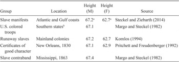
Table 1 presents evidence on heights from various antebellum sources.Footnote 3 The heights of men hover between 67.1 and 67.4 inches while those for women range from 62.7 to 62.9 inches, which are insufficiently different for practical purposes. Conceivably all sources could be biased in offsetting ways but the assembly of estimates tilts the burden of proof toward claims of the non-representativeness of the manifests. Note as well that this finding of similar averages does not foreclose the possibility of trader selectivity conditional on being on the manifests. It well could be that the average height of slaves shipped by traders was higher than the unconditional mean while those not shipped by traders was lower.
AVERAGE HEIGHTS IN INCHES OF ADULT BLACK MEN AND WOMEN FROM ALTERNATIVE SOURCES

Notes:
aAfter deleting extreme outliers using on a 1 percent trim of the sample.
bThe majority were born in border states and South Carolina.
Source:
See table.
We considered several approaches to identifying traders. Our preferred method employed a fuzzy matching algorithm that compared names and ports on ship manifests to names of traders identified by Frederic Bancroft and by Michael Tadman (Bancroft Reference Bancroft1931; Tadman Reference Tadman1989). To this list we added names from newspaper postings advertising on behalf of slave traders. The algorithm finds the “best” match in the list of traders for each slave manifest and assigns particular numerical value to the comparison of two strings, we define based on our own judgment about two cutoff values. The first value defines whether or not we consider a particular manifest to have a match, i.e., a minimum match score. The second value defines whether or not we consider a particular manifest to not have a match, i.e., a maximum match score. In addition to those matched based on comparing names and ports, we augmented this set of traders by those whose name and port appeared five or more times in nearby years in the entire collection of manifests.
We should note that this procedure does not resolve the whole set of manifests into traders and non-traders. Instead there is a sizable fraction of manifests that we exclude from the analysis because of uncertainty over the classification. Here those manifests without a good match (below the threshold for having a match but above the threshold for not having a match) and that do not appear too frequently are deemed uncertain.
Both of these thresholds for what constitutes a good match and how frequent is frequent are based on our judgments. This really is no different than other work that matches records based on non-unique identifiers. Unfortunately it is not possible to interpret the match scores as some measure of probability. This would require specifying in much greater detail the process by which errors in spellings are generated, the distribution of names of traders and non-traders, and so on. It might be useful to explore this possibility in future work, but our sense is that the gains in the formalism of the selection procedure would come at the cost of decreased transparency in what is really driving the selection. For the cutoff in terms of number of appearances, one could think about using the distribution of number of times appearing in the manifests from a sample of known traders as a way to estimate the probability that a given manifest was sent by a trader. Rather than estimate this distribution and resulting probabilities, we offer robustness checks running various specifications with different definitions of how many times a person must appear to be classified as a trader. We do not insist that there are no other reasonable thresholds but do invite other researchers to examine our code and experiment with the effects of choosing other thresholds.
We are aware of possible attenuation bias due to measurement error in determining trader status.Footnote 4 Even Pritchett and Freudenberger's approach, which used lists of slave sellers in New Orleans, had measurement error questions, and for this reason, they employed an instrumental variables strategy. Pritchett and Freudenberger wondered whether the traders were actually selling the slaves or just transshipping them and whether some of the first time sellers could be better classified as migrating planters. We face additional worries.Footnote 5 Bancroft and Tadman may have missed or misidentified slave traders, given that some slave traders chose not to advertise at all. We wonder whether enslaved crews were confounded with enslaved cargos. Missing manifests lead us to underestimate how often a name appears and how many traders there are. While relative to Pritchett and Freudenberger our approach to identifying traders almost surely has more measurement error, we do not see another solution to the question of identifying traders for this broader sample of manifests.
We argue that this tripartite classification helps to control measurement error in the trader variable. By remaining agnostic on this fraction we have more confidence in the coding of the remaining manifests. The drawback is that this causes us to drop about 39 percent of the original sample. In addition, there is an additional selection question of whether the set for which we can definitively declare to have a match or not is representative on unobservables of the whole sample. Like answering the question of the representativeness of the sample as a whole, it is difficult to provide a clear answer to the representativeness of this smaller sample.
We now consider the relationship between our trader variable and the statistical model of trader status developed by Pritchett and Freudenberger. They started from a list of known traders and non-traders at the port of New Orleans. On the basis of that list, they developed a model to predict whether a ship was sent by a slave trader based on characteristics of the cargo. They, in turn, used these characteristics as instruments for trader status with the goal of eliminating attenuation bias in estimating the relationship between trader status and heights of slaves. In particular, they found that the percentage of prime aged slaves, percentage male, and the total number of slaves on the ship were all positive predictors of being a trader (as evidenced by being on this list of traders). For a particular manifest, Pritchett and Freudenberger calculated a predicted value PV(PF) from an estimated probit model:

They transformed this variable PV(PF) by the normal CDF to calculate the “probability” a particular manifest was organized by a slave trader.
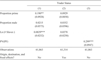
As a first pass at comparing our trader variable to Pritchett and Freudenberger's, we undertake a similar exercise by comparing the extent to which their model for identifying traders agrees with our trader variable based lists from Bancroft or Tadman, and on newspapers and repetitions. We do this in two ways. First, we re-estimate the Pritchett and Freudenberger specification using as the dependent variable our definition of trader. Note that any relationships between our trader variable and their explanatory variables of share prime, proportion male, and number slaves are not mechanical in that we do not use any of those variables to identify traders. Column 1 of Table 2 reports the results, in which we find patterns similar to those reported by Pritchett and Freudenberger (Reference Pritchett and Freudenberger1992) with both the proportion prime and the log of the number of slaves enter positively and significantly in predicting whether we classify a cargo as being shipped by a trader. While the relative magnitude to other variables (actually the only quantity identified in a probit) of the percentage male variable is reasonable, the effect of this variable is statistically insignificant. The relative magnitude between the effects of percentage prime and number of slaves is quite similar to the relative magnitude in the Pritchett and Freudenberger regression as well. In the second comparison we consider the regression coefficient of our trader variable on the PV(PF) value calculated using their reported coefficients directly. Column 3 reports the results where we find a reasonably strong correlation between the two. These results support our method of identifying traders given the success of Pritchett and Freudenberger's model to identify traders based on their list of known individuals. We emphasize that this exercise should not be interpreted as evidence for or against the quality of the instruments themselves. This is a completely separate issue that we turn to now.
REGRESSION OF THE PRITCHETT AND FREUDENBERGER EXPLANATORY VARIABLES ON OUR TRADER VARIABLE

Notes:
* p < 0.10, ** p < 0.05, *** p < 0.01.
The first two columns are results from probits, with the second including state of origin and destination fixed effects. The third column gives the correlation between our trader variable and the PV(PF) variable. All results are from a standard OLS regression including a constant. Standard errors clustered at the manifest level are in parentheses. Note that the sample size is smaller because of the fact that we are not able to classify into trader and non-trader the complete set of manifests for various reasons as noted in the text.
Source:
Slave manifest database. See text.
ESTIMATING TRADER SELECTIVITY
It would seem that the second topic we consider and the key issue of this paper, estimating the selectivity of traders, would be simple after identifying the traders. It is not. To be more precise, we want to estimate

where Xi ′ is a set of demographic controls like age or sex for a particular slave, and Heighti,j is the height of slave i on manifest j with Trader* j the true trader status of manifest j. Unfortunately, we only have access to a mismeasured version of the true trader variable, Traderj . We emphasize that all slaves on the same manifest have the same value of the Trader* j . We assume away any endogeneity issues between the explanatory variables and the residual.
We now consider a technical issue that goes back to Pritchett and Freudenberger's original work regarding the bias from measurement error in the trader variable. They argue that that measurement error will translate into estimates of the trader effect that are biased towards zero, a conclusion arrived at by analogy to the well-known result on the classical error-in-variables result for a univariate regressor. We argue that it is not so obvious the sign of the bias for two reasons. Neither of these conditions hold. First, we will need to include (Pritchett and Freudenberger do as well) additional controls beyond the trader indicator in the regression. In this case, even if all the other regressors are measured without error, there is no general result ensuring that the coefficient of interest will be attenuated. For example, even if the true trader effect were zero, in a bivariate case, if true trader status is positively correlated with the other control variable and the other control variable has a negative effect on height, then the ordinary least square (OLS) estimate will be above zero.
Second, the classical measurement error model assumes that the measurement error is independent of the true value of the regressor. This is simply impossible when the mismeasured regressor has finite support as in this case. The proposed solution in Pritchett and Freudenberger was an instrumental variables strategyFootnote 6 using some predictors of the mismeasured trader status from characteristics of the cargo on which a particular slave was shipped. Call these instruments Zi . The standard assumptions for what constitutes a valid instrument are that E Zj εi,j = 0 (exclusion) and E Zj Traderj ≠ 0 (relevance). Ignore the other regressors for now, and rewrite the model as

The IV estimator in the classical measurement error case is consistent because by assumption, the measurement error, by definition (Traderj * – Traderj ), is independent of all other variables. So that E Zj(a1(Traderj * – Traderj ) + εi,j ) = 0.
This moment will not equal zero in general because the measurement error may be dependent on other variables. It has to depend on the true value of the trader variable since the mismeasured variable has finite support. This can be rewritten as
![\[
\begin{array}
EZ(Trader^* &-Trader)={\text{PR}} (Misclass_1) E[Z\vert Misclass_1]\\
&-PR (Misclass_2) E[Z \vert Misclass_2],
\end{array}
\](https://static.cambridge.org/binary/version/id/urn:cambridge.org:id:binary-alt:20160922053101-67789-mediumThumb-S0022050716000437_eqnu4.jpg?pub-status=live)
where Misclass1 is the event where Trader * = 1, Trader = 0 and Misclass 2 is the event where Trader * = 0, Trader = 1. Note if we ran basic OLS, this moment would be –Pr(Misclass 2), the attenuation bias. This shows that the use of a “valid” instrument need not lower the magnitude of the bias and, in fact, it may actually change the sign of the bias.
Consider one of the simplest cases where the probability of each type of misclassification is equal and the instrument is positively correlated with Trader, then this bias will tend to be negative as when Trader = 1, Z will tend to be high. So, in principle, one would like to minimize the correlation between Trader, Z to minimize this problem, but that reduces the relevance of the instrument. The problem of measurement error on variables with limited support is known as classification error remains an active area of research.
Suppose we assumed that the error was classical. In this case, are they “relevant” in the first stage, and do they satisfy an exclusion restriction in the second stage? We would argue that there are reasons to doubt both of these requirements for Pritchett and Freudenberger's instruments. In particular, the relevance of their predictors in the first stage does not appear to be very robust. While the correlations are unchanged by the inclusion of year fixed effects, Column 2 of Table 2 shows that including states of origin and destination eliminates nearly all of the explanatory power of the original PV(PF) variables.Footnote 7 Second, it is not difficult to imagine situations in which some of the instruments directly predict heights of slaves in the second stage. For example, one could easily imagine that shipments that are predominantly male are intended for arduous work and, hence, face strong selection on heights. In this case, we would overestimate the effect of trader status on height per se though a certain type of selection would still be occurring.
In the end, we worry about the extent to which the “cure” of instruments is worse than the “disease” of bias due to classification error. Instead our approach presents results from a variety of specifications demonstrating the stability of the estimated effect. These specifications include: (1) OLS with our trader variable, (2) IV using our trader variable with the Pritchett and Freudenberger trader model,Footnote 8 and (3) using the predicted values from their original trader model as a proxy for trader status in an OLS specification.
The specification issue connects with the instruments question by asking what variables should be used for controls. In effect, the issue is the goal of estimation. If we are merely trying to determine whether traders shipped taller slaves, then we should just compare means without any controls. It would not matter if the reason for this difference was simply due to traders shipping on average older, and, hence taller slaves. If instead the goal is really to test the AA theorem, then it would seem to make sense to control for various demographic differences. In particular, it would not be enough for traders on average to ship taller slaves. Instead confirmation of the AA theorem would require that conditional on the slaves of a particular age, traders still continue to ship taller slaves. We view our article as mainly focused on testing the AA theorem in so far as we view the original article by Pritchett and Freudenberger to be about this as well. Because of this focus, we consider specifications that include a whole slate of controls in an attempt to identify selection by traders conditional on observable characteristics.
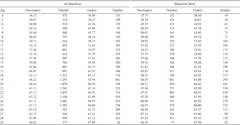
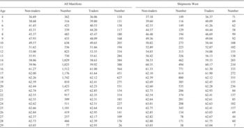
Tables 3 and 4 summarize average heights by age across trader status for males and females of all shipments and only sent from Atlantic to Gulf Coast ports (headed west). There is no important and systematic difference in heights by age for males or females, which is also true for slaves shipped from Atlantic to Gulf Coast ports.
AVERAGE HEIGHTS IN INCHES OF MALES BY AGE AND TRADER STATUSa

aAfter deleting extreme outliers using on a 1 percent trim of the sample.
Source:
Slave manifest database. See text.
AVERAGE HEIGHTS IN INCHES OF FEMALES BY AGE AND TRADER STATUSa

aAfter deleting extreme outliers using on a 1 percent trim of the sample.
Source:
Slave manifest database. See text.
REGRESSIONS
We now estimate the effect of trader status in a regression model given by
![\[
\begin{array}
Height_{it}= \alpha_0&+\alpha_1 Trader_i\\
&\sum_j \delta_j 1 [a_{it}=A_j]\\
&\sum_T \gamma_T 1[Year_{it} =Year_T]\\
&\sum_S \theta_S^0 1[State_{it}^o=State_S]+\sum_s \theta_S^d 1[State_{it}^{d}=State_S]+\varepsilon_{it}'
\end{array}
\](https://static.cambridge.org/binary/version/id/urn:cambridge.org:id:binary-alt:20160922053101-21774-mediumThumb-S0022050716000437_eqnu5.jpg?pub-status=live)
where δj , γT , θS O , γS d serve as full sets of fixed effects for ages, years, states of origin, and states of destination. We also estimate this specification separately for males and females to allow for both different height premia and differences in age-height profiles. We cluster our standard errors at the manifest level, though the differences with robust standard errors are rather minor. We will not adjust standard errors for the stochastic nature of the trader variable in the proxy specification.
A few clarifying comments regarding the specification are in order. First, note that we have repeated cross-sections rather than a panel structure. So we are estimating the age-height profile using different groups of slaves over time. Second, we choose to include both state of origin and destination fixed effects (though we will present robustness checks without them). The inclusions of both sets seem essential to us. The origin fixed effects aim to control for possible differences in the local populations of slaves. The destination fixed effects, on the other hand, aim to control for potentially different uses of slaves in their final destination and, hence, different general selective pressures for height.
Baseline Results
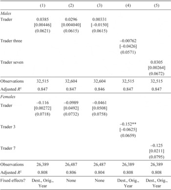
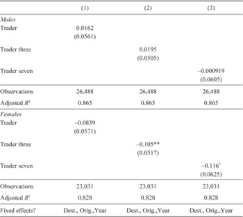
Table 5 provides results for males and females, respectively, for three different definitions of trader. The first columns utilize our preferred method with various sets of fixed effects included, and the later columns employ variations on the number of voyages under the same name (and port of origin) in determining whether someone was a trader. The two variations are whether a name is repeated more than three times and another where it must be repeated more than seven times. We find very little evidence for selectivity on the part of the traders. Across all of the specifications, the trader variable is never statistically significant and the point estimates are not meaningful in a practical sense for males or females. To emphasize, these are precisely estimated null effects. These results constitute our response to the second issue: we find no evidence for trader selectivity. We also report the analysis with our original trader definition that resolved all manifests into either traders or non-traders rather than leaving a fraction uncertain. The results reported in square brackets below the baseline ones are even more attenuated, which we take as supporting our approach here of leaving this intermediate set out in the main specification. In the Appendix, we offer results trimming the height outliers in the sample. Results are unaffected here.
OLS REGRESSION OF SLAVE HEIGHTS ON OUR TRADER VARIABLES

Notes:
* p < 0.10, ** p < 0.05, *** p < 0.01.
Standard errors in parentheses, clustered at the manifest level. Trader is our preferred measure of trader status. Besides matching to newspaper advertisements, Trader three (seven, respectively) counts all name and port pairs that appear three or more (seven, respectively) times as a trader. Destination and Origin fixed effects are for the states of the port of origin and destination. The top panel is for male slaves and the bottom is for female slaves. In brackets, we report the results using the indicator for trader status in our original JEH article. Relative to the preceding regressions, this trader variable resolves all manifests into either trader or non-trader with no indeterminate manifests.
Source:
Estimated from the slave manifest database. See text.
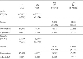
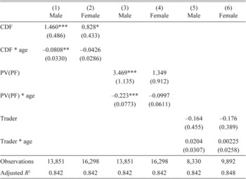
Table 6 reports the results from some other definitions of trader status for males and females. The first two columns use the PV(PF) variable as a proxy for trader status. In our sample, the mean and standard deviation of PV(PF) are −0.485 and 0.14, respectively. There is evidence for a differential effect of trader status on height for males and females. The PV(PF) variable is positive and statistically significant whether or not location fixed effects are included. That said, the impact of the trader variable is quite small, ranging from 0.42 to 1.12 inches and averaging 0.71 inches, relative to the four inches of catch-up growth to be explained. In one specification for females with no fixed effects we find a large effect of approximately 1.12 inches.
OTHER SPECIFICATIONS FOR TRADER STATUS ON HEIGHT OF SLAVES

Notes:
Standard errors in parentheses.
* p < 0.10, ** p < 0.05, *** p < 0.01.
The first two columns are OLS specifications using the predicted values from the Pritchett and Freudenberger trader model as a proxy for trader status. Column 3 is an IV specification where we use the predicted values from the trader model in Pritchett and Freudenberger as an instrument for our trader status variable. Column 4 is an IV specification where we re-estimate in the first stage the relationship between Pritchett and Freudenberger's instrument and our trader variable. Location fixed effects are a full set of state of origin and destination fixed effects. Standard errors are clustered at the manifest level.
Source:
Estimated from the slave manifest database. See text.
The last two columns in Table 7 reports results from IV specifications. In the third column, we use the PF(PV) constructed variable as an instrument for our trader variable. In the fourth column, we run an IV using the Pritchett and Freudenberger predictors of trader status as instruments (in effect, re-estimating the relationship between the instruments and our trader variable in the first stage). As we noted in discussing those results, there is worry about weak instruments. While our trader variable agreed with the basic predictions of the Pritchett and Freudenberger trader model, the instruments fail the weak instruments test. The F-statistic for the test of joint significance is less than four. So we are skeptical about the reliability of the estimated effects, and this shows with very large standard errors and implausibly large effects of trader status. The key is the inclusion of the state of origin and destination fixed effects, which eliminate much of the relationship between the instruments and our trader variable.
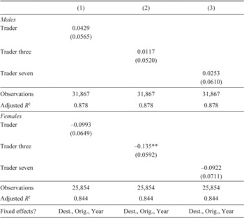
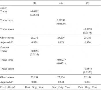
ROBUSTNESS CHECK EXCLUDING PRE-1850 MANIFESTS

Notes:
* p < 0.10, ** p < 0.05, *** p < 0.01.
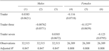
Standard errors in parentheses, clustered at the manifest level. Trader is our preferred measure of trader status. Besides matching to newspaper advertisements, Trader three (seven, respectively) counts all name and port pairs that appear three or more (seven, respectively) times as a trader. Destination and Origin fixed effects are for the states of the port of origin and destination. The top panel is for male slaves and the bottom is for female slaves.
Source:
Estimated from slave manifest database. See text.
We consider an additional robustness check here where we restrict attention to shipments before 1850. Tadman (Reference Tadman2000, p. 1566) states that the surviving manifests are a “very incomplete record of the coastal traffic.” Now there is no reason to believe that whatever is missing is a non-random sample of the overall set of records. However, missing manifests would lead to potential undercounting and misclassification of manifests with regard to trader status since we use the number of appearances as a condition for inclusion. The issue seems most problematic after 1850. So we rerun our basic specifications dropping all manifests after 1850. Table 7 reports these with results very similar to the baseline specifications. In particular, there is no observable selection on male heights by traders and, if anything, the selection is negative for females.
Differences between Age Groups
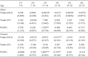
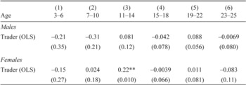
It might be argued that trader selectivity should only apply to select age categories, in particular, children and adolescents. Table 8 disaggregates this trader effect for males and females by age group. In theory, the overall null effect of trader status could be the result of a composition bias with different age groups experiencing different trader effects that wash out. We report the results for the basic OLS specification with our trader variable, the IV specification with PF(PV) as the instrument, and an OLS regression with PF(PV) as a proxy for trader status. All include state of origin and destination fixed effects.
EFFECT OF TRADER STATUS ON HEIGHTS FOR VARIOUS AGE GROUPS

Notes:
Standard errors in parentheses.
* p < 0.10, ** p < 0.05, *** p < 0.01.
Standard errors are clustered at the manifest level. All regressions include the following fixed effects: age, year, state of origin, and state of destination. The first row is an OLS specification using our trader variable. The second row is an IV specification using our trader variable and the PF(PV) variable as the instrument. The third row is an OLS specification using the PF(PV) variable as a proxy for trader status.
Source:
Estimated from slave manifest database. See text.
The results reported in Table 8 eliminate composition bias as an explanation for the catch-up growth because evidence of trader selectivity is lacking for any of the age groups or genders using our trader variable. In the first two columns with the OLS specification and the IV specification, there are no significant effects. There does, however, appear to be a slight negative effect for female slaves between ages 15 and 18, but it is small. This is also not the group for which Pritchett and Freudenberger found the largest effect. Using PV(PF) variable as a proxy variable for status in the third row, we find some evidence for trader selectivity in particular groups. Whatever effect of trader status, it is concentrated among adolescents for males and females between 11 and 14. We remain skeptical about the significant effects for this specific age group, particularly in light of inconsistent results for other specifications.Footnote 9 Furthermore, false positives are a possibility given we are running multiple regressions across various age groups and genders. As purely a matter of chance, one would expect to find a statistically significant result when estimating this many regressions (even if the null were true). Furthermore, for the other age group of females, 15–18, with a positive effect, we get negative point estimates using our trader variable. In conclusion we find no evidence of systematic differences in selection across demographic groups as defined by age or gender.
Differences across Space
Here we investigate the relationship between trader selectivity and geography. In particular, we ask whether distance shipped matters for trader selectivity following Pritchett (Reference Pritchett1997). The claim that slaves shipped greater distances would be subject to greater selectivity is a prediction of the AA theorem, in so far as shipping distance is correlated with shipping costs. Komlos and Alecke (Reference Komlos and Alecke1996) argued that the wedge driven between the prices of high and low productivity slaves by shipping costs were small. We now provide some quantitative evidence on their claim. We calculate shipping distances for the largest ports of origin and destination as noted in our earlier paper. These include: Alexandria, Virginia; Baltimore, Maryland; Charleston, South Carolina; Galveston, Texas; Mobile, Alabama; Norfolk, Virginia; New Orleans, Louisiana; Pensacola, Florida; Richmond, Virginia; Savannah, Georgia; and Jacksonville, Florida. We calculate straight-line distances, which is easy to do and provides a reasonable approximation for shipments within the same body of water. For shipments between an Atlantic and a Gulf Coast port, we calculate the distance between the origin and Key Largo, Florida (roughly the tip of Florida) and add that to the distance from Key Largo to the destination.
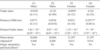
We are interested in the interaction between the trader status variable and distance. We include distance itself as an additional control. Results for males and females are separately reported in Table 9. We consider two specifications, ones with and without state of origin and destination fixed effects. We find no differential effects of shipments sent longer distances by traders. The effect of distance alone is positive though not statistically significant and quite small except for the specification with no location fixed effects for women. In this case, the difference in average heights for slaves shipped to New Orleans from Jacksonville versus Baltimore, say, is about 0.2 inch. This distance effect is consistent with the results in Pritchett (Reference Pritchett1997), however, the interaction between the trader and distance variable is consistent with the Komlos and Alecke argument that the wedge between the price of high productivity and low productivity slaves due to shipping costs was small.
DIFFERENCES IN TRADER SELECTIVITY BY DISTANCE SHIPPED

Notes:
* p < 0.10, ** p < 0.05, *** p < 0.01.
Standard errors are clustered at the manifest level. All regressions include age and year fixed effects. All specifications use our preferred definition of trader. The sample sizes are smaller as we restrict attention to the largest ports as noted in the text.
Source:
Estimated from slave manifest database. See text.
We have also estimated fully saturated models with origin and destination fixed effects, and the results are basically the same, as one can see by comparing Table 9 with Appendix Table 1. We were not able to run one with origin x destination fixed effects since this requires the estimation of more than 5,000 indicator variables.
EXPLAINING THE DIFFERENCES BETWEEN OUR RESULTS AND PRITCHETT AND FREUDENBERGER
What explains the difference between our results and the original results in Pritchett and Freudenberger of trader selectivity? There are a number of possibilities. First, they had data only for shipments to New Orleans versus the entire collection of manifests in our case. Second, we would argue that there is no reason to believe that measurement error in the trader variable necessarily leads to an attenuation bias for the estimated effect. Third, their regressions were misspecified in the use of their instruments (the “Forbidden Regression” problem) and the validity of their instruments themselves. Fourth, Pritchett and Freudenberger included the interaction between trader and age in a linear fashion. (This seems to be in tension with the fact that they included a full set of age fixed effects as well.) Finally, there is the question of how manifests are classified as traders.
To address these possibilities, Table 10 attempts to “reproduce” the Pritchett and Freudenberger results. For all of these regressions, we restrict attention to shipments with a destination of New Orleans. We also basically employ the same specification, splitting the population into males and females and using the age group 4–17. The only difference is the inclusion of state of origin fixed effects for us rather than the port of origin fixed effects that they used. The first two columns use the normal CDF of the transformed PV(PF) variable that they employed. Here we find a pattern similar to their results, if slightly attenuated. The second two columns re-estimate the regression using the untransformed Pritchett and Freudenberger variable that we employed in the earlier specifications. We find that the trader effects appear stronger than the transformed case and in our previous regressions where we examined the trader variable separately for different age groups. For now, we at least conclude that the effects reported in Pritchett and Freudenberger are not due to a Forbidden Regression problem. Finally, the last two columns report estimates for our preferred trader variable. We find as before, no effect.
REPRODUCING THE PRITCHETT AND FREUDENBERGER RESULTS

Notes:
* p < 0.10, ** p < 0.05, *** p < 0.01.
The first two columns use the normal CDF of transformed PV(PF) values as in the original Pritchett and Freudenberger paper. The second two columns use the non-transformed values, and the final two use our trader variable. Trader definition is based on whether name is listed in newspaper or if name appears five or more times. The sample sizes are smaller because of the restriction to New Orleans shipments as well as the limits on age of 4–17.
Source:
Estimated from slave manifest database. See text.
Where does that lead us in understanding the difference between our results and Pritchett and Freudenberger's? First, their restriction to the port of New Orleans was not decisive. Nor was the linear interaction between age and trader. What does matter is whether port of origin fixed effects should be included. We argue that these fixed effects are warranted to control for differences in the characteristics of the local slave population. The inclusion of these fixed effects calls into question the validity of the instruments. That said, the trader selectivity in Pritchett and Freudenberger was present without instrumenting. So what is crucial is how the trader variable is defined. Our method leads to much lower estimates of the degree of selectivity.
CONCLUSIONS
Our earlier work using slave manifests to investigate the interregional movement concluded that professional traders transported a majority of the individuals shipped from exporting to importing states, giving considerable scope to trader preferences in biasing measured heights. Theoretical explanations anticipate opposing effects created by mixing short or tall individuals preferred by slave traders. Which force dominated is an empirical matter. Depending upon age and sex, the average difference in stature of slaves moved by these two groups was at most a small fraction of an inch. Hence, we conclude that there is no systematic height biased imposed by traders that could explain the large catch-up growth.
We cannot prove that the manifests themselves are representative. Our goal is to cast doubt on one source of possible non-representativeness. For the sake of argument, assume that these manifests were representative. What hypotheses remain in attempting to explain the catch-up growth? First, potential biases arising from the repeated cross-sectional nature of the data rather than a true panel do not seem large enough. The pattern of catch-up existed within all regions so catch-up growth could not be a problem of composition bias. Also, simulations indicate that selective mortality imparted a small upward bias to the heights by age during the teenage years, but this explains only a tiny portion of the four-inch catch-up. It should be noted that the considerable catch-up growth of young children adopted from poor into rich countries demonstrates that the slave growth pattern is biologically possible.Footnote 10 Previous work has shown that one major disease that could have stunted the growth of slave children in the form of hookworm infestations among teenagers explains at most a small share of the catch-up growth (Coelho and McGuire Reference Coelho and McGuire2000; Steckel Reference Steckel2000). What remains then is selective nutrition on the part of slave owners. In future work, we attempt to provide positive evidence for the nutrition hypothesis by linking slave heights to the prices of cotton and pork.
Appendix A: Estimates with a Fully Saturated Model
Here we report the results from a “fully saturated” model where we include a full set of port of origin and port of destination fixed effects. This allows for the fixed effect by port to differ between outgoing and incoming shipments. Note however that this is not the same as including the full Cartesian product of ports of origin and destination. Given the number of ports we have, this specification is computationally infeasible. We use our baseline trader variable and estimate the effect by age group. Results are reported below and should be compared to those in Table 9. We are still unable to detect any economically or statistically significant selection by traders and for at least half the categories for males and females, the selection is towards shorter slaves.
DIFFERENCES IN TRADER SELECTIVITY BY DISTANCE SHIPPED USING A FULL SET OF ORIGIN AND DESTINATION FIXED EFFECTS

Appendix B: Results for Trimmed Datasets
We offer additional robustness checks by trimming the 1, 3, and 5 percent tails of the standardized height distribution. Outliers have the potential to, at least, lead to inflation of the standard errors and statistically insignificant estimates. Rather than calculate these percentiles age by age and trimming 1 percent of each age distribution, we transform heights into z-scores by subtracting the average and dividing by the standard deviation age by age and then trim the resulting distributions of z-scores by gender. This trimming is for the set of slave heights on manifests that are either classified as a trader or non-trader. The results show little difference with the baseline case. Standard errors are slightly smaller though the “problem” was not too large of standard errors but too small of a point estimate of the trader effect. Even after trimming tails, the average difference in heights between slaves shipped by traders relative to non-traders is still trivial. Appendix Tables 2, 3, and 4 display the results for these different cuts, respectively. We do these for our three different versions of the trader variable. As is evident, results do not seem to be driven by outliers. Results are stable across these three cuts and not substantially different from the results for the full sample.
OLS REGRESSION OF SLAVE HEIGHTS TRIMMING THE 1 PERCENT TAILS OF THE STANDARDIZED HEIGHT DISTRIBUTION BY GENDER

OLS REGRESSION OF SLAVE HEIGHTS TRIMMING THE 3 PERCENT TAILS OF THE STANDARDIZED HEIGHT DISTRIBUTION BY GENDER

OLS REGRESSION OF SLAVE HEIGHTS TRIMMING THE 5 PERCENT TAILS OF THE STANDARDIZED HEIGHT DISTRIBUTION BY GENDER