1. Introduction
Macroeconomic adjustment (or stabilization) policies, i.e., policies to reduce inflation and increase welfare, often require the implementing government to take politically unpopular or even costly measures. Beyond an economically consistent program, the political economy literature argues that the outcome of such policies critically depends on credibility, i.e., whether private agents believe that the implementation of the adjustment will persist and be carried out (Dornbusch (Reference Dornbusch1991), Drazen and Masson (Reference Drazen and Masson1994)). Consequently, the success of adjustment should crucially depend on the extent of cohesion among members of the executive (“Government unity,” henceforth) and the government’s capacity to enact its policy program via legislative support (Government strength,” henceforth).Footnote 1 The empirical literature indeed provides evidence for the view that both dimensions matter for the outcome of adjustment (see, e.g., Sargent (Reference Sargent and Sargent2013), Hamann and Prati (Reference Hamann and Prati2002), Dollar and Svensson (Reference Dollar and Svensson2000), Herwartz and Theilen (Reference Herwartz and Theilen2021), Ardagna (Reference Ardagna2004)).
In this paper, I explore an additional aspect in this context, namely the relevance of popular support for the government and/or its leader (“Government stability,” henceforth). Specifically, I examine whether a lack of government stability affects macroeconomic adjustment programs.
To do this, I leverage the failed adjustment of the Macri government (2015–19) in Argentina. Specifically, I exploit an insightful case in this context: In a session of the Chamber of Deputies (lower house of Argentina’s National Congress) on Dec. 14, 2017, a reform of the pension system was supposed to be approved. The reform was a key element of the adjustment since the pension system significantly contributed to the country’s high government expenditures and quasi-fiscal deficit.Footnote 2 The need for a fiscal correction was further reinforced by tax cuts and increased government spending, as well as by the government’s electoral victory that the markets considered as a deadline for finally starting the fiscal consolidation (Sosa-Padilla and Sturzenegger (Reference Sosa-Padilla and Sturzenegger2023), Sturzenegger (Reference Sturzenegger2019)). By linking pensions to inflation and wage growth, the reform significantly contributed to the fiscal correction but implied also a decrease of pensions and slower pension growth, respectively (see IMF (2016), IMF (2022)). Therefore, the reform proposal generated resistance among large parts of the society and induced mass protests in the run-up to the session, resulting in violent clashes with public security forces.Footnote 3 Due to the incidents, the session was unexpectedly suspended by order from the government, and the pension reform was not approved on that day. In a subsequent effort, the Congress approved the reform on Dec. 19, 2017, with a small margin of 128 to 116 votes.
I argue that the outlined event adversely impacted the program’s credibility since it highlighted the lack of government stability and low level of popular support and consensus among relevant socioeconomic groups regarding the adjustment agenda. This negatively affected market expectations regarding the government’s ability to implement challenging policies and increased the probability that reforms would be postponed, not implemented, or even reversed at some point in time.
Using daily data on the nominal exchange rate (XR), which reflects market expectations regarding future policies and the government’s ability to carry out the adjustment, as outcome variable, I apply the Synthetic Control Method (SCM) to a sample of 39 upper-middle income countries.Footnote 4 The SCM, developed by Abadie and Gardezabal (Reference Abadie and Gardezabal2003), Abadie et al. (Reference Abadie, Diamond and Hainmueller2010) and Abadie et al. (Reference Abadie, Diamond and Hainmueller2015), constructs a counterfactual for how the nominal XR would have evolved in the absence of the outlined event on Dec. 14, 2017. I find that the event caused a nominal XR depreciation of 15% over seven weeks. The estimates are statistically significant and remain robust across numerous robustness checks and alternative subsamples. In addition, although with a lag, I obtain very similar estimation results when I use country risk, measured by sovereign spreads, as alternative outcome variable. I further observe comparable treatment effects when I restrict the analysis to comparison countries that are similar to Argentina in terms of macroeconomic performance. The XR depreciation reflects the adverse consequences of a shock to government stability. It shows the negative impact on market expectations regarding the government’s ability to implement adjustment policies in the long run and, ultimately, on the program’s credibility.
Government stability matters for adjustment policies for several reasons. First, adjustments often imply losses for certain sectors and conflict with the political preferences of relevant parts of the society. Given that policymakers respond to political demand and act under the threat of being punished at the polls, governments with low levels of support may tend to implement less adjustment than necessary and delay or even reverse challenging reforms (Alesina et al. (Reference Alesina, Favero, Giavazzi, Alesina, Favero and Giavazzi2019), Alesina and Drazen (Reference Alesina and Drazen1991), Dornbusch and Edwards (Reference Dornbusch, Edwards, Dornbusch and Edwards1991), Blanchard (Reference Blanchard1985)). The expectation of policy reversals discounts the impact of the (pre-announced) adjustment path and weakens the transmission to investment (Afonso and Galiani (Reference Afonso and Galiani2025)). In addition, the success of adjustments crucially depends on the expectation that policies are maintained in the long run. Implementing policies that move too fast are likely to cause retaliation at some (future) point in time. This constrains the future policy space to execute the adjustment, thereby reducing the program’s credibility (Drazen and Masson (Reference Drazen and Masson1994)). In line with this, since the probability of policy reversals and delays is low under broad support, this credibility advantage shifts down the short-run Philips curve more quickly for a given initial inflation level, resulting in smaller sacrifice ratios (Caporale and Caporale (Reference Caporale and Caporale2008)). Finally, high levels of government stability and the inclusion of key actors in the reform process reduce uncertainty regarding their cooperation and compliance, and enhance the acceptance of the reforms (Acemoglu and Robinson (Reference Acemoglu and Robinson2001), Black et al. (Reference Black, Kraakman and Tarassova2000), Bunce (Reference Bunce2001), Alexeev (Reference Alexeev1999)).
My paper adds to the literature on macroeconomic adjustment and policy reform.Footnote 5 Specifically, I speak to the political economy literature on the determinants of policy credibility and the success of adjustment. Even though there is some theoretical work related to the role of government stability (Dornbusch (Reference Dornbusch1991), Alesina and Drazen (Reference Alesina and Drazen1991), Drazen and Masson (Reference Drazen and Masson1994), Blanchard (Reference Blanchard1985), Velasco (Reference Velasco and Velasco2008), Tabellini and Alesina (Reference Tabellini and Alesina1990)), this aspect has received only limited attention in the empirical literature. I contribute to this strand of the literature by showing that events during adjustments, which highlight a lack of government stability, can lead to a sizable currency depreciation. This reflects the negative impact on market expectations regarding the government’s ability to implement challenging policies in the long run and on the adjustment’s credibility. Accordingly, my paper also adds to the more comprehensive empirical literature highlighting that government strength and unity are key determinants of the success of adjustment (e.g., Sargent (Reference Sargent and Sargent2013), Hamann and Prati (Reference Hamann and Prati2002), Dollar and Svensson (Reference Dollar and Svensson2000), Herwartz and Theilen (Reference Herwartz and Theilen2021), Ardagna (Reference Ardagna2004)). The vast majority of the related empirical work relies on panel data analysis of multiple countries and years, and on proxy variables measuring government strength, unity, or stability. For example, studying 51 episodes of inflation stabilizations in 31 countries, Hamann and Prati (Reference Hamann and Prati2002) show that the probability of success is positively linked to the strength of the executive authority, measured by the institutional constraints on the executive branch of government. Ball and Rausser (Reference Ball and Rausser1995) document for a sample of 138 countries that countries with more political freedoms and rights are more successful in stabilizing inflation in the long run. The authors argue that, in these countries, it takes longer to build the necessary consensus to successfully stabilize. However, once a consensus is achieved, adjustments are more durable than in repressive regimes. Grier et al. (Reference Grier, Lin and Ye2015) provide evidence for 90 countries (1975–2011) that higher levels of political fractionalization are associated with longer delays in fiscal adjustments. Sargent (Reference Sargent and Sargent2013) argues that the adjustment program of Margaret Thatcher in the 1970s failed because it was opposed by the Social Democrats, Labour Party and even by the Conservative Party itself. Therefore, a “once-and-for-all, widely believed, uncontroversial, and irreversible regime change” was not believed to take place. While these papers benefit from a higher degree of external validity, their results may be biased due to identification problems such as measurement error, reverse causality or omitted variable bias.
To address (some of) these concerns, I adopt a case study design and assess the impact of a plausibly exogenous shock to government stability on the nominal XR, employing the SCM (Abadie and Gardezabal (Reference Abadie and Gardezabal2003)). By using high frequency data, I track the temporal sequence of a specific event and rule out similar treatments in comparison units. Given that the outcome is a financial price which flexibly responds to all available information and reflects market expectations on the government’s ability to implement the policies in the long run, my research design allows me to identify the causal effect on the credibility of macroeconomic adjustment. I conduct the analysis in the Argentine context—a country whose long history of financial crises and failed stabilizations makes it an ideal laboratory for examining the research question.Footnote 6 Importantly, since the reform was ultimately approved a few days later, the specific chronology of the event makes it plausible that the identified effect primarily captures the adverse consequences of a lack of government stability and not of a lack of government unity and/or strength. Typically, these variables are strongly correlated which makes it challenging to disentangle their individual role in the context of adjustment.
The remainder of the paper is organized as follows: Section 2 provides background information on the adjustment program of the Macri government and on the reform of the pension system. Section 3 presents the data and research design. Section 4 presents the baseline results and the results of several robustness checks. Section 5 discusses some alternative explanations for the failure of the adjustment program which are advanced in the literature. The section also corroborates the external validity of my findings and discusses the potential role of confounding events in Argentina and the US. Section 6 concludes.
2. Background
This section outlines the adjustment program of the Macri government and the events surrounding the reform of the pension system in Dec. 2017.
2.1 Adjustment program of the Macri government
On Nov. 22, 2015, Mauricio Macri was elected as Argentina’s new president by a narrow margin of 2.68 percentage points. Macri won the first presidential runoff since the return to democracy in 1983. The newly elected government was confronted with a challenging economic environment: Growth rates declined, inflation was high, and budget and current account deficits increased (see Figure FF1). To correct these imbalances, especially to reduce inflation, the Macri government started to implement a macroeconomic adjustment program right after taking office on Dec. 10, 2015. A key feature was the introduction of a multi-year inflation targeting scheme with a floating XR. Capital controls were removed and the government fixed a path to reduce central bank transfers to the Treasury. Furthermore, the government pursued a gradualistic fiscal policy. With real expenditures held constant and fiscal revenues rising through economic growth, the budget deficit should remain steady at –2% of GDP. Through these measures, inflation was projected to increase from 25% to 40% in the first year (2016), mainly due to the reduction in subsidies, and decrease to 5% until 2019. Output was projected to grow in all years of the presidential term (Sturzenegger (Reference Sturzenegger2019)).
Two and a half years later, in Jun. 2018, the government and the IMF agreed upon a Stand-By Agreement of over 50 billion US dollars which constituted the largest single arrangement in the IMF’s history. Unlike the economic forecasts of the government, growth rates were negative, inflation increased, and the currency strongly depreciated (see Figure FF2). The failure of the economic policy program of the Macri government is also illustrated by Figure 1. The graph plots the daily official XR (black solid line) and black market (or parallel) XR (black dashed line) between the Argentine peso and US dollar during the Macri presidency (Dec. 10, 2015 – Dec. 10, 2019). The official XR increased from 13.75 to 60.51 Argentine pesos per US dollar (340%
 $\uparrow$
). The XR gap (black bars) between the official and the black market XR also increased since the black market rate increased from 14.36 to 70 Argentine pesos per US dollar (390%
 $\uparrow$
).Footnote
7
Argentina: Exchange rate (Dec. 10, 2015 – Dec. 10, 2019).
Notes: Official (black solid line) and black market nominal XR (black dashed line) at a daily frequency. The XR is measured in units of Argentine pesos per one US dollar. The XR gap (black bars) is the difference (in %) between the official and the black market XR. Time period: Dec. 10, 2015 – Dec. 10, 2019. Data sources: La Nación (2022) (black market XR), BCRA (2023) (official XR).

2.2 The reform of the pension system
The case of reform. Contrary to the original program, fiscal policy was initially loose, with tax cuts and increased government spending generating a fiscal cost of around 4.3% of GDP in 2017. Amongst others, corporate income taxes, export taxes and taxes on small and medium-sized enterprises and on the automotive sector were reduced, and the minimum taxable income was increased (Sturzenegger (Reference Sturzenegger2019)). The need for a fiscal correction was not only due to this initial fiscal expansion but also due to the government’s electoral victory in the mid-term elections in Oct. 2017, considered by the markets as the deadline to initiate the fiscal adjustment (Sosa-Padilla and Sturzenegger (Reference Sosa-Padilla and Sturzenegger2023)).
A key feature to correct the fiscal deviation from the adjustment program and address, at least partly, the long-term disequilibria in Argentina’s public finances was the reform of the pension system.Footnote
8
Mainly driven by subsidies and pension outlays, primary expenditures doubled between 2005 and 2015, and total pension payments accounted for 45% of total federal spending in 2015 (
 $\approx$
9.2% of GDP in 2015). The deficit of the pension system amounted to 2.8% of GDP and was estimated to increase until 2,066 to around 40% of 2015 GDP in net present value (NPV) terms (IMF (2016)). Pensions were also relatively high compared to other countries. For example, in 2021, replacement rates amounted to around 90% of the average wage (OECD average: 58%). The ratio of pensioners to the population older than 65 years was also well above the OECD average. As a result, pension expenditures were relatively large and more than double the mean of comparable emerging market economies and other Latin American countries (IMF (2022)). The significant weight of pension payments in overall government spending also contributed to the low flexibility of public expenditures and their specific character challenged the credibility of the adjustment: Due to the backward indexation of pensions, lower inflation rates mechanically increased real pension expenditures.Footnote
9
Therefore, without a reform, a sustained disinflation would automatically lead to a fiscal expansion, inconsistent with the policy program (Sturzenegger (Reference Sturzenegger2019)). Pension indexation generated around 0.3% of GDP of additional pension spending during the (temporary) disinflation in 2017. The total cost to reach an annual inflation rate of 5% implied around 1% of GDP of additional annual pension spending (Afonso and Galiani (Reference Afonso and Galiani2025)).
Parts of these imbalances originated from former policies which were (partly) funded through social insurance and pension contributions. For example, the number of beneficiaries of family allowances increased from 3 to 11 million between 2005 and 2015, mainly due to the introduction of universal child allowances for 3.7 million children. In the same period, 2.9 million people without prior contributions were allowed to receive pensions, accounting for around 30% of pension expenditures (IMF (2016), IMF (2022)).
The events on Dec. 14, 2017. The reform that the Macri government proposed in 2017 primarily consisted in a change of the indexation formula, linking pensions to inflation and wage growth and shortening the period of pension actualization from six to three months. Projections of the IMF suggested that indexing pensions and actualizing past wages to the real inflation would contribute to stabilize, at least to some extent, the pension system’s deficit but also implied a decrease of initial pensions and slower pension growth, respectively. The rise in pension spending would be reduced by around 20% of GDP in NPV terms. Together with a gradual increase of women’s retirement age from 60 to 65 years, the increase of the pension system’s deficit until 2,066 would be reduced to almost zero (see IMF (2016)).
The reform plan generated broad resistance. Surveys indicated that around 80% of the people were against a modification of the indexation formula for the purpose of reducing the fiscal deficit. Around 50% of the population generally did not support the reform proposal (Ambito Financiero, 2017)).
On Dec. 14, 2017, the Chamber of Deputies voted on the reform proposal. Before, the bill had been approved by the Senate. In the run-up to the session, parts of the opposition, together with trade unions and social movements, mobilized large-scale protests which culminated in violent clashes with public security forces on the streets outside the Congress in Buenos Aires. Members of Congress, journalists, and citizens were injured, and dozens of people arrested. The opposition accused the government of infiltrating people into the Congress to approve the reform. Due to the incidents, the session was suddenly suspended by order from the government, and the reform was not approved on that day. Nevertheless, after debating for more than 12 hours, the Chamber of Deputies approved the reform on Dec. 19, 2017, with a small margin of 128 to 116 votes. Again, there were large protests in the whole country and the biggest trade union (General Confederation of LabourFootnote 10 ) declared a national strike for 24 hours. Members of the government accused the protesters of destabilizing the government and carrying out a coup d’état. Violent clashes on the streets in Buenos Aires resulted in more than 160 injured and 60 arrested persons (see, e.g., Cué & Barreiro (Reference Cué and Barreiro15.12.2017), BBC (19.12.2017), Cué & Molina (Reference Cué and Molina19.12.2017), Serra (Reference Serra19.12.2017)).
Government stability. I argue that the outlined event adversely impacted the program’s credibility by highlighting the lack of government stability and low levels of popular support and consensus among relevant socioeconomic groups. This negatively affected market expectations on the government’s ability to implement challenging policies in the long run and increased the probability that reforms would be postponed, not implemented, or even reversed. Furthermore, even though the reform was ultimately approved, the fact that the government held no majority in either of the two chambers of Congress further constrained the policy space to execute the adjustment.
The lack of government stability is also illustrated by the evolution of the Trust in Government (ICG) index. The ICG index, developed by the University Torcuato di Tella and available at a monthly frequency, measures, amongst others, the public perception in Argentina regarding the government’s ability to resolve the problems of the country.Footnote 11 Herrera et al. (Reference Herrera, Ordoñez and Trebesch2018) document that the ICG index is tightly linked to the ICRG government stability index, a commonly used metric of government stability across countries (Acemoglu et al. (Reference Acemoglu, Johnson and Robinson2001), Alfaro et al. (Reference Alfaro, Kalemi-Ozcan and Volosovych2008)). They also show that the ICRG government stability index captures very well the dynamics of government popularity, at least in countries where public opinion polls are available. In Dec. 2017, the ICG index dropped by around 20% relative to the previous month. It was the largest decrease during the Macri presidency that was surpassed, before then, only in May 2008 (−23%) and during the sovereign default in 2001/02. Amongst others, the strong decrease can be attributed to the way in which the pension reform was carried out (University Torcuato di Tella (2023)).
The next section introduces the data which I use to evaluate the impact of the outlined event on the adjustment program of the Macri government.
3. Data and research design
In this section, I introduce the data and my empirical approach to study the research question.
3.1 Outcome variable and data
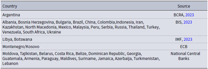
I use the (log) nominal XR as outcome of interest, measured in units of domestic currency per one US dollar. Thus, a rise of the XR indicates a nominal depreciation of the domestic currency against the US dollar. I employ daily data of the official nominal XR for the period between the day after the Argentine mid-term elections in 2017 (Oct. 22, 2017) and Feb. 2, 2018. This gives me a sufficiently large pre- and post-treatment period of seven weeks. XR data of Argentina come from BCRA (2023). Most of the XR data of the comparison countries come from the BIS (2023), which I complemented with data from IMF (2023a) and individual central banks.Footnote 12 I restrict the empirical analyses to upper-middle income and transition economies according to UN (2020) and World Bank (2021). In doing so, my sample entails 39 similar comparison countries with respect to economic development. Table T1 shows the comparison countries included in the sample and the country-specific data sources.
The nominal XR is a suitable outcome variable for my analysis because, given that it is a forward-looking asset price free from price rigidities and given that financial prices incorporate all available information and news, it reflects market expectations regarding future policies (Fama (Reference Fama1998), Chan (Reference Chan2003), Engel and West (Reference Engel and West2005), Lustig et al. (Reference Lustig, Roussanov and Verdelhan2011), Itskhoki and Mukhin (Reference Itskhoki and Mukhin2025)). Thus, if the government was not expected to carry out the reforms due to a lack of government stability, corresponding XR changes reflect the expected probability of a non-implementation (or a reversal) of the adjustment. In this sense, the effect of shocks to government stability on policy credibility can be inferred from variations of the nominal XR. Importantly, the information content of the XR and, thus, the analysis would be biased by foreign exchange (FX) interventions and restrictions of capital flows. However, the Macri government entirely lifted capital controls on Dec. 17, 2016, and the XR floated virtually freely until Mar. 2018 (Sturzenegger (Reference Sturzenegger2019)).
Besides these theoretical considerations, using the XR as main outcome has also practical advantages. First, the XR is determined each day on the FX market. Other variables which directly measure government stability (e.g., ICG index, ICRG government stability index) or expectations regarding the adjustment, most prominently survey data, are only available at a lower frequency. This also applies to other potential outcomes, particularly macroeconomic indicators such as inflation or GDP, which typically exhibit a high degree of serial correlation. Second, there is no cross-country information regarding similar events which may have occurred in comparison countries. By employing daily XR data, I mitigate the probability that comparison countries experienced a (similar) treatment at the same time. Using more aggregated data (e.g., monthly observations) may confound the analysis.
Instead of the nominal XR, I may consider country risk as an alternative outcome variable. A common measure for country risk is the spread between the yields of US dollar–denominated bonds issued by emerging market countries and the yields of (risk-free) US Treasury bonds (“EMBI spreads”). Other scholars also use sovereign spreads in their analyses. For example, Ciro and de Mendonça (Reference Ciro and de Mendonça2016) show for Colombia (2004–15) that greater monetary policy credibility is linked to lower spreads. Obstfeld and Taylor (Reference Obstfeld and Taylor2003) analyze sovereign spreads to study the credibility of XR regimes for different countries between the 1870s and 1930s. Unfortunately, daily spread data free of charge exist for only a few countries. Nevertheless, I obtain similar results when I run the SCM with sovereign spreads as outcome (see Subsection 4.3).
3.2 Research design
To estimate the counterfactual, I use the SCM, developed by Abadie and Gardezabal (Reference Abadie and Gardezabal2003), Abadie et al. (Reference Abadie, Diamond and Hainmueller2010), and Abadie et al. (Reference Abadie, Diamond and Hainmueller2015). Using a weighted average of available control units, the SCM provides an estimation of how the variable of interest (here: nominal XR) of the treated unit (here: Argentina) would have developed in the absence of the treatment (here: event on Dec. 14, 2017).
More formally, consider variable
 $E_{it}$
observed in country
 $i=1,\ldots ,N$
over the time period
 $t=1,\ldots ,T$
.
 $T_0 \in [1,T)$
is the number of pre-treatment periods.
 $E_{it}^0$
denotes the potential outcome of country
 $i$
at time
 $t$
without treatment.
 $E_{it}^1$
is the potential outcome of country
 $i$
at time
 $t$
when unit
 $i$
is exposed to the treatment from
 $T_0+1$
to
 $T$
. The treatment is assumed to have no impact on the outcome variable prior to the treatment. That is,
 $E_{it}^0=E_{it}^1$
for
 $t \in \{1,\ldots , T_0 \}$
and all
 $i \in \{1,\ldots , N \}$
. Assume that country
 $i=1$
(here: Argentina) is treated whereas countries
 $i=2,\ldots ,N$
serve as potential control units (“Donor pool,” henceforth).
I aim to estimate the treatment effect for Argentina in the post-treatment period. That is, for
 $i=1$
and
 $t\gt T_0$
, I estimate:
 \begin{equation} \tau _{1t} = E_{1t}^1 - E_{1t}^0 . \end{equation}
Given that the outlined event on Dec. 14, 2017 represents the treatment,
 $E_{1t}^1$
is observed and
 $E_{1t}^0$
is unobserved in the post-treatment period, i.e.,
 $E_{1t}^1=E_{1t}$
for
 $t \in \{ T_0+1,\ldots ,T \}$
.
 $E_{it}^0$
is observed for the control units in
 $t \in \{1,\ldots , T \}$
. Thus, to estimate
 $\tau _{1t}$
, given by
 \begin{equation} \tau _{1t} = E_{1t} - E_{1t}^0 , \end{equation}
one needs to estimate
 $E_{1t}^0$
. I follow Abadie and Gardezabal (Reference Abadie and Gardezabal2003), Abadie et al. (Reference Abadie, Diamond and Hainmueller2010) and Abadie et al. (Reference Abadie, Diamond and Hainmueller2015) and use a weighted average of untreated units from the donor pool (“Synthetic Argentina”/“Doppelganger,” henceforth):
 \begin{equation} \hat {\tau }_{1t} = E_{1t} - \sum _{j=2}^{N} w_j E_{jt}, \end{equation}
for
 $t \in \{T_0+1,\ldots ,T\}$
as an estimator for
 $\tau _{1t}$
. Thus, the counterfactual is a weighted sum of a subset of donor pool countries. The weights,
 $w_j$
, which are allowed to vary across countries, are constructed by minimizing the distance between the pre-treatment covariates of the treated country and untreated donor pool countries. Following Abadie et al. (Reference Abadie, Diamond and Hainmueller2010), I impose
 $w_j \geq 0$
and
 $\sum _{j=2}^N w_j =1$
.
To implement the SCM, I follow Doudchenko and Imbens (Reference Doudchenko and Imbens2016) and use only lagged pre-treatment outcomes but no further covariates. I deviate from other papers which use, e.g., different covariates in addition to all lagged pre-treatment outcomes (Billmeier and Nannicini (Reference Billmeier and Nannicini2013), Stearns (Reference Stearns2015), Bohn et al. (Reference Bohn, Lofstrom and Raphael2014)). Other studies include covariates and the average of the pre-treatment outcomes (Kleven et al. (Reference Kleven, Landais and Saez2013)). However, as shown by Kaul et al. (Reference Kaul, Klößner, Pfeifer and Schieler2022), using all lagged pre-treatment outcomes in addition to other covariates renders all covariates irrelevant and implies that the SCM is determined by optimizing only the pre-treatment fit with respect to the outcome of interest. This can bias the synthetic control estimator because the more covariates truly matter for future values of the outcome of interest, the more biased the estimated treatment effects become when these covariates are disregarded in the analysis (Kaul et al. (Reference Kaul, Klößner, Pfeifer and Schieler2022)). The authors argue that this reduces the efficiency of the synthetic control by introducing a small-sample bias. It also violates the principle of using all available variables to predict the outcome of interest, thereby deviating from the SCM’s original purpose (see also Gardeazabal and Vega-Bayo (Reference Gardeazabal and Vega-Bayo2017)).
4. Results
I now present my baseline results and the results of several robustness checks.
4.1 Baseline results
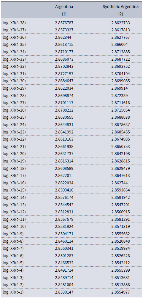
Figure 2 shows the baseline estimation results. Panel (a) displays the time series of the nominal XR of Argentina (black solid line) and of the doppelganger economy (black dashed line). Panel (b) displays the XR gap between them. Prior to the outlined event, both time series exhibit a high degree of co-movement, demonstrating that Synthetic Argentina provides a convincing counterfactual. This allows me to estimate the causal impact of the event on the nominal XR.Footnote 13 I quantify the treatment effect on the XR by comparing the actual evolution of the nominal XR with the counterfactual XR of Synthetic Argentina following the outlined event. The XR of Argentina and Synthetic Argentina immediately start to diverge after the event, with the XR gap gradually widening over time. Quantitatively, my results suggest that the event led to a nominal XR depreciation of 15% over seven weeks.Footnote 14
This estimated number is economically significant, considering, e.g., the literature that identifies currency crises based on thresholds of annual devaluations of 15% (Reinhart and Rogoff (Reference Reinhart and Rogoff2011)) or 25% (Frankel and Rose (Reference Frankel and Rose1996)).
The SCM assigns Jamaica (26.4%), Malaysia (24.8%) and Montenegro/Kosovo (19.6%) the largest country weights, accounting together for 70.8% of the dynamics of Synthetic Argentina. Turkey (11.9%), Paraguay (6.3%), South Africa (6.0%) and Colombia (5%) account for the rest of the dynamics.Footnote 15

The results are in line with Alesina and Drazen (Reference Alesina and Drazen1991) who formally study the politico-economic determinants of delays in the adoption of fiscal adjustment programs.Footnote 16 They present a rational heterogeneous agents model of delayed stabilizations and derive the expected time of stabilization as a function of characteristics of the economy, including the degree of political polarization. In the model, adjustments are delayed due to a “war of attrition” between different socioeconomic groups with conflicting distributional objectives that disagree on who has to bear the burden of adjustment policies.Footnote 17 The war of attrition ends, thereby allowing stabilization, when certain groups concede and allow their political opponents to decide on the burden’s allocation. They formally show that when the burden of stabilization is distributed relatively unequally, i.e., in countries with a high degree of polarization or a lack political cohesiveness, the expected benefit from waiting for the opponents to concede and bear a disproportionate share of the adjustment’s burden exceeds the costs, thereby delaying stabilizations. More broadly, the model underlines the role of political consolidation as a critical element of credibility, i.e., the credibility and success of an adjustment is contingent upon the extent of political support it is able to generate. Given that the degree of political support shifts over time and is affected by political events, an adjustment program may experience a transition from a good equilibrium, characterized by effective performance, to a bad equilibrium, in which the program becomes unviable. As costs accumulate over time, previously supportive groups may be compelled to concede their backing, thereby rendering a program unfeasible.
The role of political consolidation is therefore also strongly related to the role of policymakers’ commitment as another key element of credibility (see, e.g., Rodrik (Reference Rodrik1989)). Policymakers with a strong commitment are less likely to abandon or reverse policy reforms. Consequently, when the public is uncertain about the policymakers’ commitment due to a lack of political support and, hence, the probability to abandon or reverse policy reforms is high, adjustments are less likely to succeed.
Chow test. To check whether the event represents a structural break in what had been the XR, I employ the Chow test (break test for a known date). Specifically, I regress the difference between the XR of Argentina and Synthetic Argentina,
 $Y_t$
, on a dummy variable,
 $D_t$
, that is equal to one after Dec. 14, 2017, and equal to zero before:
 \begin{equation} Y_t = \beta _0 + \beta _1 D_t + \varepsilon _t \end{equation}
Table 1 shows the estimation result, highlighting that the XR difference after the event is significantly different from the pre-treatment period.
Chow test

Table 1. Long description
A table with three rows and four columns. The table compares the XR difference between Argentina and synthetic Argentina. The columns are labeled Dt, 0.100***, 0.007, N, 75, and R2, 0.728. The first row shows Dt, 0.100***, and 0.007. The second row shows N and 75. The third row shows R2 and 0.728.
XR effect of political events. Research shows that political events can translate into significant XR effects. For example, Costa, et al. (Reference Costa, Dhingra and Machin2024) and Manasse, et al. (Reference Manasse, Moramarco and Trigilia2024) show that, following the Brexit vote on Jun. 23, 2016, the Sterling depreciated within one day by, on average, 6.7% against major currencies, ranging between 4.3% (Polish zloty) and 11.1% (Japanese yen). Consistent with this, Kalemli-Özcan and Varela (Reference Kalemli-Özcan and Varela2025) find that political uncertainty is an important determinant of systematic deviations from the Uncovered Interest Rate Parity (UIP) across countries and moves very closely with this UIP risk premium. Consistent with this, they show that the nationalization of Argentina’s pension fund in Oct. 2008 induced an expected XR depreciation of 12 pp. over 12 months. Boer and Rieth (Reference Boer and Rieth2023) show that, by raising producer prices and weaking domestic demand, uncertainty about trade policy depreciates the domestic currency. Itskhoki and Mukhin (Reference Itskhoki and Mukhin2025) document that, immediately after the invasion of Ukraine on Feb. 24, 2022 and the imposition of sanctions on Russia, the Russian ruble lost half of its value. However, the XR returned to its pre-war level within weeks, appreciated 30% by June, and gradually depreciated over the following year, resulting in a 20% depreciation relative to the pre-war level. Their calibrated model captures well the depreciation of the ruble by 20% over two years after the start of the war.Footnote 18 Balima (Reference Balima2020) finds that coups d’état depreciate the nominal effective XR by, on average, about 0.35%, which is twice the average sample depreciation rate. In addition, the likelihood of a currency crisis increases by 2 pp., which represents about 90% of the average currency crisis probability. Studying the impact of US presidential election TV debates on intraday XR returns of 96 currencies (1996–2016), de Boer et al. (Reference de Boer, Eichler and Rövekamp2024) find that currencies of countries highly integrated with the US via exports significantly depreciate if the election probability of the protectionist candidate increases during the debate. Quantitatively, currencies of highly integrated countries with bilateral exports to the US of 25% of their GDP depreciate by 8 basis points if the protectionist candidates’ election probability increases by 2 pp., which accounts for more than the half of the standard deviation of the XR returns.Footnote 19 Other related papers exploit news shocks regarding Donald Trump’s presidency to identify the effect of anticipated protectionist measures on XR. Wolfers and Zitzewitz (Reference Wolfers and Zitzewitz2016) document an appreciation of the Mexican peso and Canadian dollar during the first presidential TV debate in 2016, when the perceived election probability of Trump was reduced. Tweets by Trump on possible import tariffs (Matveev and Ruge-Murcia (Reference Matveev and Ruge-Murcia2024), Jeanne and John (Reference Jeanne and John2024)) and days with trade war shocks (Carlomagno and Albagli (Reference Carlomagno and Albagli2022), Chen et al. (Reference Chen, Fang and Liu2023)) are associated with an appreciation of the US dollar.Footnote 20 Berdiev et al. (Reference Berdiev, Kim and Chang2012) find for a panel of 180 countries (1974–2004) that left-wing governments, democratic institutions, and CB independence are associated with a greater probability of choosing a flexible XR regime. Flexible regimes are also more likely to be established prior to elections. Cermeño et al. (Reference Cermeño, Grier and Grier2010) show for a panel of nine Latin American countries that real effective XR depreciations intensify after presidential elections, with a significantly higher post-election XR volatility. Barbiero et al. (Reference Barbiero, Farhi, Gopinath and Itskhoki2018) find that unanticipated changes in border adjustment taxes significantly move XR by almost the size of the tax adjustment.
4.2 Permutation test
To verify that our baseline results capture the causal effect of the event on the XR, I follow Abadie et al. (Reference Abadie, Diamond and Hainmueller2010) and apply the SCM to all countries in the sample (“Permutation test”). That is, I proceed as if each of the donor pool countries would have experienced the treatment instead of Argentina, thereby verifying that the results are not driven by chance. The main idea behind this test is that our baseline estimate for Argentina captures the causal effect of the event as long as comparable treatment effects do not arise from fictitious interventions in donor pool countries.
Figure 3 shows the results of the permutation test. The black solid line plots the baseline XR gap of Argentina, depicted in panel (b) of Figure 2. The dashed lines display placebo XR gaps which emerge from the permutation test. That is, they show, for each donor pool country, the gap between the time series of the actual XR and of the synthetic control. Since, for some donor pool countries, the pre-intervention dynamics cannot be well reproduced by a combination of other countries, the figure does not contain placebos with a poor pre-treatment fit. Specifically, I exclude donor pool countries with a pre-treatment root mean squared prediction error (RMSPE) of more than two times that of Argentina. Argentina’s XR gap clearly stands out and is the largest among all 29 placebo gaps.


Alternatively, we evaluate the results of the permutation test by computing, for Argentina and each donor pool country, the relative RMSPE, defined as the ratio between the pre- and post-treatment RMSPE (RMSPE
 $_{post}$
/RMSPE
 $_{pre}$
). Panel (a) in Figure F1 shows that Argentina’s ratio of 26.73 is particularly large compared to the donor pool countries.Footnote
21
Panel (b) shows the distribution of relative RMSPEs, with Argentina appearing at the far right. If the treatments were allocated randomly among the countries, the probability of obtaining the same ratio would be
 $1/30=0.033$
.
Taken together, Figures 3 and F1 indicate that our baseline estimates in Figure 2 capture the causal effect of the outlined event on the nominal XR.
4.3 Robustness checks
Adjusted donor pools. In my baseline model, I consider around 40 donor pool countries. One concern may be that many of these countries are economically much less volatile than Argentina and may therefore not represent suitable comparison units. Table TT2 shows the average annual inflation rate, nominal XR variation and GDP growth, as well as their standard deviations, for Argentina (columns (1)–(2)) and for the baseline donor pool (columns (3)–(4) between 2010 and 2016. It can easily be seen that the inflation rates and XR variations of the donor pool countries were, on average, lower and GDP growth higher than in Argentina. Therefore, since its economic performance substantially differs from that of the donor pool economies, Argentina may not fit within the full set of countries used to construct the doppelganger economy.
To tackle this concern, I create adjusted donor pools which contain only countries with high inflation, large XR variations or low growth rates (2010–16). The first two adjusted donor pools encompass countries with (average) inflation rates and XR variations above the sample mean of the baseline donor pool. The third donor pool contains only countries with growth rates below the sample mean. For example, I create a high inflation pool that contains all donor pool countries with an average inflation rate exceeding 7.58%, which is the sample mean of the baseline donor pool. Columns (5)–(6) of Table TT2 show that the countries which constitute the adjusted donor pools are macroeconomically more similar to Argentina. For example, while average inflation and XR variation across the baseline donor pool economies amounted to 7.58% and 7.3%, compared to 29.25% and 24.36% in Argentina, inflation and XR variations of the adjusted donor pool economies were, on average, equal to 20.56% and 16.53%. Put differently, the countries comprising the adjusted donor pools are more comparable to Argentina with respect to macroeconomic performance.
I re-estimate my baseline model with these adjusted donor pools. Panel (a) in Figure 4 shows the baseline XR gap together with the XR gaps from the synthetic controls which use the adjusted donor pools. Although the XR gap estimated with high inflation countries is smaller, it is still sizable and implies a nominal XR depreciation of 10% over seven weeks following the outlined event. Regarding the other adjusted donor pools, the post-treatment XR gaps are very much the same as in the baseline model.
Robustness: Selection of donor pool countries.
Notes: Results of the robustness check that accounts for comparable macroeconomic performance of Argentina and donor pool countries. Data sources: BIS (2023), BCRA (2023), IMF (2023a), individual central banks (daily nominal XR, see Table T1); IMF (2024a), Kehoe and Niccolini (Reference Kehoe and Niccolini2021) (inflation, 2010–16); own calculations using World Bank (2024) (nominal XR variation, 2010–16); IMF (2024b) (real GDP growth, 2010–16).

Figure 4. Long description
Two line graphs depict the treatment effect of macroeconomic adjustment policies over time for different donor pools. Panel A shows the treatment effect for adjusted donor pools 1/2, while Panel B shows the treatment effect for adjusted donor pools 2/2. Each graph has a vertical axis labeled Treatment effect and a horizontal axis labeled with dates ranging from November 1, 2017, to February 28, 2018. Panel A includes lines for Baseline, High inflation pool, Low growth pool, and Depreciation pool. Panel B includes lines for Baseline, Inflation, GDP growth, and XR variation. Both graphs show a vertical dashed line around December 2017, indicating a significant event or change. In both panels, the treatment effect remains relatively stable before the dashed line but shows an upward trend afterward. The lines for different donor pools exhibit varying degrees of increase, with some pools showing a more pronounced rise in treatment effect than others. The graphs illustrate the impact of different macroeconomic factors on the effectiveness of adjustment policies over time.
I further restrict the donor pool to countries which lie in the upper decile of inflation, nominal XR variation and GDP growth across donor pool economies. Column (7) of Table TT2 shows that the average inflation rate across these countries is 30.42% (Argentina: 29.25%) and the average XR variation is 26.40% (Argentina: 24.36%). Thus, the past macroeconomic performance of these countries in terms of inflation and XR volatility is almost the same as that of Argentina. The only exception is GDP growth (−0.74% vs. +2.30%). Panel (b) in Figure 4 shows the results of the robustness check. Although the XR gaps estimated with the adjusted donor pools are smaller as in the baseline model, and more dispersed as in panel (a), they still suggest that the event resulted in an XR depreciation of around 10% over seven weeks.
Influential control units. Are my baseline findings driven by influential control units? To address this concern, I check whether donor pool countries with positive country weights in the baseline model disproportionately drive the estimated treatment effect. I iteratively drop these countries from the donor pool and re-estimate my baseline model. The left panel of Figure 5 shows that the XR gaps estimated with these restricted donor pools (black dashed lines) are identical to the baseline XR gap (black solid line).
Robustness: Influential donor pool countries.
Notes: Results of the robustness check that accounts for influential donor pool countries and deals with potentially confounding events in the donor pool countries. In the left panel, the XR gaps for the restricted donor pools (black dashed lines) are obtained by iteratively excluding countries from the donor pool which received positive country weights in the baseline model. In the right panel, the black dashed lines show the XR gap obtained from the subsample that excludes all countries from the donor pool which received positive country weights in the baseline model, as well as the XR gap obtained from the subsample that excludes the countries which received the three major weights in the baseline model (Jaimaica, Montenegro/Kosovo, Malaysia). Data sources: BIS (2023), BCRA (2023), IMF (2023a), individual central banks (see Table T1).

In addition, given that around 70% of Synthetic Argentina is made up of three donor pool units (Malaysia, Jamaica, Kosovo/Montenegro), I simultaneously exclude these three countries from the donor pool and re-run the baseline specification. I also simultaneously exclude all donor pool countries that receive a positive weight in the baseline finding. In this way, I further address the concern that potentially confounding events in the (main) donor pool countries around the same date as the outlined event, rather than the suspension of the congressional vote in Argentina, explain the XR effect. The right panel of Figure 5 shows that the XR gap is almost identical to the baseline XR gap.
Taken together, the figures underline that my main findings can be attributed to the outlined event on Dec. 14, 2017, and are not confounded by unrelated events in donor pool countries.
Spillovers. The baseline model estimates the treatment effect under the assumption that the outlined event solely affected Argentina, without influencing other countries in the donor pool. The assumption would be violated in the presence of interdependencies through which the event in Argentina had spillover effects on other countries. One source of spillovers may come from trade linkages. According to the INDECFootnote 22 (INDEC (2023)), more than 50% of Argentine imports in 2017 and 2018 came from Brazil (25%), China (18%) and the US (11%). Around 30% of total exports during that period also went to those countries. In addition, the baseline estimates may also be biased by spillovers to other Latin American economies due to, e.g., regional contagion.
Robustness: Spillovers and LAC economies.
Notes: Panel (a) shows the results of the robustness check that accounts for spillovers to other countries due to trade linkages and to other LAC economies. Panel (b) shows the results of the robustness check that restricts the donor pool to LAC economies. Data sources: BIS (2023), BCRA (2023), IMF (2023a), individual central banks (daily nominal XR, see Table T1); INDEC (2023) (Trade of Argentina, 2017–18.)

Figure 6. Long description
Two line graphs depict the treatment effect on the nominal exchange rate over time, comparing baseline and specific country groups. Panel A shows the results of the robustness check that accounts for spillovers to other countries due to trade linkages and to other Latin America and the Caribbean economies. Panel B shows the results of the robustness check that restricts the donor pool to Latin America and the Caribbean economies. Both graphs have the x-axis labeled with dates ranging from November 1, 2017, to February 2, 2018, and the y-axis labeled with the treatment effect. The vertical dashed line indicates a significant event or change point around December 2017. In both panels, the red line represents the baseline, and the black line represents the specific country groups. In Panel A, the black line represents countries excluding China, Brazil, and Latin America and the Caribbean. In Panel B, the black line represents Latin America and the Caribbean economies. Both graphs show a relatively stable treatment effect before the dashed line, followed by an increase in the treatment effect after the dashed line, with some fluctuations. The treatment effect rises more sharply and reaches higher values in the post-event period, indicating a nominal depreciation of the domestic currency against the US dollar.
I tackle these concerns by excluding donor pool countries with a share of more than 10% of Argentina’s imports and exports in 2017 and 2018 (Brazil, China). I further exclude all economies from Latin America and the Caribbean (LAC). Panel (a) in Figure 6 presents the results of this robustness check, indicating that the XR gap is virtually identical to the baseline XR gap. Similarly, I re-estimate the baseline model for a restricted donor pool which only contains LAC economies. Panel (b) presents the results. Although the XR gap is somewhat smaller than in the baseline model, it still shows an economically significant XR depreciation of over 10%.
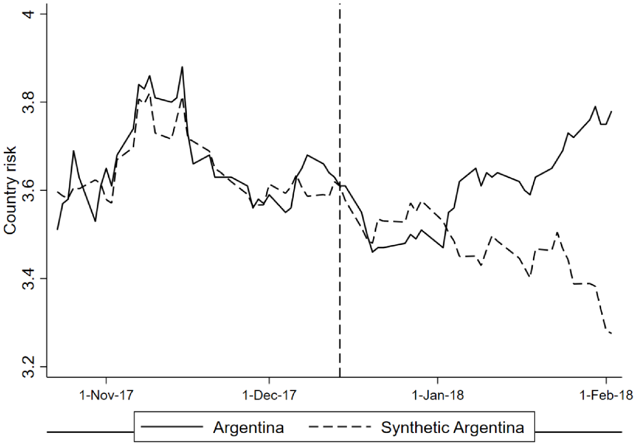
Alternative outcomes. Instead of the nominal XR, I may consider country risk as an alternative outcome variable, measured by EMBI spreads. Even though it is challenging to obtain comprehensive high frequency data, the Central Bank of the Dominican Republic provides daily data on EMBI spreads for Argentina and 15 other Latin American countries. I re-estimate my baseline model for the same time period using EMBI spreads as outcome and their entire pre-treatment path as predictors.
Figure F2 displays the time series of Argentina (black solid line) and Synthetic Argentina (dashed black line). Prior to the treatment, the spreads closely co-move and exhibit a similar evolution. Then, albeit with some delay, the spread of Argentina gradually diverges from that of Synthetic Argentina. Relative to Synthetic Argentina, the spread increases by 51 basis points (15%
 $\uparrow$
) over seven weeks after the outlined event.Footnote
23
Time placebos. I run a time placebo test and artificially backdate the treatment to each of 15 pre-treatment periods, thereby exposing Argentina to fictitious treatment dates. The idea behind this test is that the baseline XR effect captures the causal effect of the event as long as comparable effects are not measured at fictitious treatment dates.
Figure F3 shows the results of the time placebo test. The black solid line plots the actual XR of Argentina and the black dashed line plots the counterfactual XR of Synthetic Argentina. Each dashed gray line displays the XR of Synthetic Argentina for one time placebo. Despite heterogeneity, the figure shows that the synthetic controls obtained from this exercise diverge from the actual XR only after the original treatment date.
Institutions and exchange rate policies. In a further robustness check, I account for exchange rate policies. Specifically, I exclude donor pool countries with a fixed XR regime according to the latest year of observation (2016) of the broad classification of Ilzetzki, et al. (Reference Ilzetzki, Reinhart and Rogoff2019) (IRR, 2018). Alternatively, I include only countries with the same de facto XR regime in 2017 as Argentina—namely managed floats—according to the revisited XR regime classification of Levy-Yeyati and Sturzenegger (Reference Levy-Yeyati and Sturzenegger2024) (LYS, 2023). Relatedly, I use the same classification and exclude all countries without floating XR in 2017.
Next, I account for institutional differences across countries and restrict the donor pool to economies with comparable institutional quality, approximated by the level of democracy. First, I include only democracies in 2017, using the democracy index of Gruendler and Krieger (Reference Gruendler and Krieger2021). Second, I draw on the 2023 democracy report of Varieties of Democracies (V-Dem) which provides country-specific information on the political regime between 2012 and 2022. The resulting donor pool only entails electoral democracies—just like Argentina.
Panel (a) in Figure F4 shows the results of the first and panel (b) the results of the second robustness check. Both tests yield almost the same XR gaps as in the baseline model. Thus, the results are unaffected when I only consider comparison countries with comparable XR regimes or institutional quality.
5. Discussion
So far, the results robustly show that the outlined event on Dec. 14, 2017 caused a meaningful XR depreciation, reflecting the negative impact on the adjustment’s credibility and on market expectations regarding the government’s ability to implement adjustment policies in the long run. In this section, I discuss three alternative explanations for the breakdown of the program: (1) The tightening of international financial conditions, (2) the change of inflation targets by the government on Dec. 28, 2017, and (3) the drought in Argentina between the end of 2017 and mid-2018. Lastly, I discuss external validity and the concern of confounding events in Argentina and the US.
5.1 Alternative explanations
International financial conditions. The (ongoing) tightening of international financial conditions, especially after the FED’s taper tantrum in 2013, may have disproportionately affected countries reliant on foreign funding and with weak macroeconomic fundamentals, such as Argentina (Uribe and Yue (Reference Uribe and Yue2006), Bernanke (Reference Bernanke2017), Avdjiev and Takáts (Reference Avdjiev and Takáts2019)). To address this concern, I re-estimate the main specification for different subsamples of the baseline donor pool, restricting the analysis to those countries which are similarly exposed to innovations in global financial markets due to their reliance on foreign funding and/or weak fundamentals. The first subset contains countries with a current account deficit, and the second subset contains countries with a primary deficit in any year between 2016 and 2018. In the third donor pool, I consider countries with a central government debt of less than 25% of GDP in any year between 2016 and 2018.Footnote 24 Figure 7 displays the baseline XR gap (black solid line) and the XR gaps from this robustness check (dashed black lines), demonstrating that there are virtually no differences between them.
Robustness: International financial conditions.
Notes: Results of the robustness check that restricts the donor pool to countries which are similarly exposed to unexpected changes in international financial conditions due to their reliance on foreign funding and/or weak macroeconomic fundamentals. Data sources: BIS (2023), BCRA (2023), IMF (2023a), individual central banks (daily nominal XR, see Table T1); IMF (2023b) (central government debt, % GDP); IMF (2023c) (primary balance, % GDP); IMF (2023d) (current account balance, % GDP).

28D hypothesis. Another explanation comes from Sturzenegger (Reference Sturzenegger2019) who argues that the adjustment failed due to a change of the central bank’s inflation target, announced by the Macri government in a press conference on Dec. 28, 2017. Specifically, he argues that, due to the large share of backwardly indexed public expenditures, a successful disinflation challenged the financing of the budget deficit and required additional fiscal consolidation measures. To avoid this, the government announced a change of the central bank’s inflation target which constituted an intervention in the central bank’s autonomy to independently choose policy targets and apply monetary policy instruments. This, in turn, was perceived by the markets as an unexpected institutional change of monetary and fiscal policy which resulted in the loss of the adjustment’s credibility (“28D hypothesis,” henceforth). Note that the 28D hypothesis is not very different from the argument advanced in this paper since the policy shift was due to a disagreement among the fractions of the government regarding the speed of adjustment and should have been a reaction to the outlined event on Dec. 14, 2017.
To test the 28D hypothesis, I reassign the treatment to Dec. 28, 2017, and re-run the SCM. Figure 8 shows an increase in the XR gap starting on Dec. 14, i.e., before the government announced the change of the inflation target. In addition, similar to the Chow test, I regress the difference between the nominal XR of Argentina and Synthetic Argentina on a binary dummy that is equal to one between Dec. 14 and Dec. 28, 2017 and equal to zero before. Table TT3 shows that the XR difference is not significantly different between both periods. Thus, the event on Dec. 28, which should have been a reaction to the event on Dec. 14 and should have additionally heightened the ongoing pressure on the XR, can be seen as a complementary explanation for the failure of the adjustment.
Drought in 2017/18. Between the end of 2017 and mid-2018, Argentina experienced the worst drought in 70 years, with an economic cost of approximately four billion US dollars (
 $\approx$
0.8% of 2018 GDP) (Centre for Research on the Epidemology of Disasters (2023), Bert et al. (Reference Bert, de Estrada, Naumann, Negri, Podesta, de los Milagros Skansi, Spennemann and Quesada2021)). Due to Argentina’s economic dependence on commodity production and export and given that the drought mainly affected those regions which produce most of the country’s agricultural commodities (provinces of Buenos Aires, Córdoba, Santa Fe, the Pampas and Entre Ríos), it should have also affected the XR. However, due to the diffuse nature of this event, this alternative explanation is difficult to test. Although I cannot completely discard this hypothesis, the chronology of the event makes it less plausible: The drought started in Nov./Dec. 2017, and the most intense phase was between Jan. and Apr. 2018. Especially after Feb. 2018, a large share of land was affected by extreme and exceptional drought conditions (Centre for Research on the Epidemology of Disasters (2023), Bert et al. (Reference Bert, de Estrada, Naumann, Negri, Podesta, de los Milagros Skansi, Spennemann and Quesada2021)).
5.2 External validity and confounding events in Argentina and the US
External validity. The outlined event may exhibit a high degree of particularity, limiting the extent to which broader generalizations can be drawn. I now corroborate the external validity of my findings and examine the XR impact of large corruption scandals which arguably represent plausibly exogenous shocks to government stability in the context of (expected) macroeconomic adjustments.Footnote 25
Robustness: 28D hypothesis.
Notes: Result of the robustness check that reassigns the treatment to Dec. 28, 2017. The black vertical line shows the treatment assignment on Dec. 28, 2017. The gray vertical line indicates the original treatment date on Dec. 14, 2017. Data sources: BIS (2023), BCRA (2023), IMF (2023a), individual central banks (see Table T1).

First, I leverage the release of the Spagnuolo-audios during the macroeconomic adjustment implemented by the Milei government in Argentina since Dec. 2023. The program critically centers on a crawling peg and fiscal consolidation, immediately eliminating a national government budget deficit of 5% of GDP (Obstfeld (Reference Obstfeld2026), Obstfeld (Reference Obstfeld2025)). The policies helped to reduce inflation, with monthly inflation dropping from 25% to 2–3% within one year, and overall economic activity recovered to some extent. Manufacturing production stabilized but at a lower level. However, over time, disinflation and economic growth, particularly in manufacturing, stagnated (Figures FF4 and FF5).Footnote 26
A major event occurred on Aug. 19, 2025, with the release of the so-called Spagnuolo-audios. Diego Spagnuolo was the former head of the National Disability Agency (ANDIS), responsible for, amongst others, the procurement and distribution of medications for disabled people through the public healthcare system. In the audios, Spagnuolo describes an alleged bribery and corruption scheme in which public contracts with pharmaceutical laboratories, arranged through ANDIS, were allegedly inflated by around 8%. Parts of the commissions were then channeled to prominent members of the Milei government. In particular, 3% of the total contract values were allegedly allocated to Karina Milei, the President’s sister and General Secretary of the Presidency.Footnote 27 The case seriously challenges the government’s central promise to shift the burden of the adjustment to the corrupt political caste.
Second, I leverage Operation Lava Jato (OLJ) which constituted Brazil’s largest anti-corruption and anti-money laundry investigation, resulting in over 360 convictions, 400 plea bargains and around 30 corporate leniency agreements (Ferraz et al. (Reference Ferraz, Moura, Norden and Schechtman2025)). OLJ took place in an economic context of relatively large fiscal deficits and high inflation rates (Table TT4), requiring some sort of adjustment policy. It started in Mar. 2014 as a local money laundering investigation. Within a few months, the corruption scandal encompassed the state-owned oil company, Petrobras, and Brazil’s largest construction companies which formed a cartel of Petrobras’ contractors, with about 59 billion Brazilian reais (11.4 billion US dollars) in Petrobras contracts. Pre-defined shares (1–5%) of overbilled construction contracts (e.g., oil refineries, offshore exploration vessels) were allegedly diverted to political actors and private construction companies (Ferraz et al. (Reference Ferraz, Moura, Norden and Schechtman2025), Valarini and Pohlmann (Reference Valarini and Pohlmann2019), Netto (Reference Netto2016), Campos, et al. (Reference Campos, Engel, Fischer and Galetovic2021), Fisman et al. (Reference Fisman, Sarkar, Skrastins and Vig2020), Ros and Taylor (Reference Ros and Taylor2022)).
On Sep. 6, 2014, Brazil’s leading weekly newsmagazine, Veja, published parts of the testimony of Paulo Roberto Costa (PRC). PRC, a former member of Petrobras’ executive board, was the first high-level executive to provide an inside account of the corruption scheme and supplied a list of political figures involved in the scandal. The testimony is considered as a major turning point in OLJ, transforming the case from a corporate fraud investigation into a major political corruption scandal. Top-tier politicians and business leaders, including the federal government, congressmen, state governors, senators, ministers, and the former CEO of Latin America’s largest construction firm (Odebrecht), were involved in what became the largest corruption scandal ever uncovered in Latin America (Ferraz et al. (Reference Ferraz, Moura, Norden and Schechtman2025)).
Nominal XR and sovereign spreads around Operation Lava Jato and Spagnuolo-Audios.
Notes: The left panel shows the nominal XR and EMBI spreads before and after the release of the Spagnuolo-audios (time period: Aug. 01 – Sep. 30, 2025). The XR is measured in units of Argentine pesos per one US dollar. The black dashed vertical line indicates the day of the release of the Spagnuolo-audios (Aug. 19, 2025). The gray dashed vertical line indicates the day of the announcement of financial support to Argentina, made by the US secretary of the treasury, Scott Bessent. The right panel shows the nominal XR and EMBI spreads before and after the release of the testimony of principal witness in OLJ, P. R. Costa (time period: Apr. 01, 2014 – Feb. 27, 2015). The XR is measured in units of Brazilian reals per one US dollar. The black dashed vertical line indicates Sep. 5, 2014. On Sep. 6, 2014, Brazil’s leading weekly newsmagazine, Veja, published part of the testimony given to police by the principal witness, P. R. Costa, a former member of Petrobras’ executive board and principal witness in OLJ. Data sources: FRED, BCRA, Banco Central de la Republica Dominicana (2026).

Figure 9 shows the time series of the nominal XR and sovereign spreads around the release of the Spagnuolo-audios (panel (a)) and the publication of the testimony of PRC (panel (b)). The XR and sovereign spreads remained constant prior to the event but significantly increased by 16.1% and 108% over six weeks (panel (a)) and by 14.6% and 62.4% over 25 weeks (panel (b)). Taken together, both panels support the view that plausibly exogenous shocks to government stability in the context of (expected) adjustments negatively affect policy credibility.
Please note in panel (a) the drop of the XR and sovereign spread after Sep. 22. On this day, US treasury secretary, Scott Bessent, stated that “Argentina is a systematically important US ally in Latin America, and the US Treasury stands ready to do what is needed within its mandate to support Argentina. All options for stabilization are on the table.” The financial turbulances induced the US government to provide a swap facility of 20 billion US dollar to BCRA and to directly intervene in the Buenos Aires FX market with 2.5 billion US dollars (Obstfeld (Reference Obstfeld2026)).
Confouding events in Argentina and the US. A final concern is whether the XR effect can be attributed to other events, either in Argentina or in the US, rather than to the suspension of the congressional vote.
First, potentially confounding events in Argentina may have induced investors to revise their expectations, anticipating fiscal difficulties independently of the pension reform events. To address this, I rely on the prominent LatinNews Country Database to manually search for major economic (E) and political (p) news in Argentina in Oct., Nov. and Dec. 2017 (until Dec. 14, 2017).Footnote 28
Table TT5 summarizes the main events. During these months, fiscal difficulties appear to have played a minor role and most news do not suggest that investors revised their expectations in advance of the outlined event. For example, in October, INDEC reports that economic growth accelerated from 0.3% in 2017 Q1 to 2.7% in 2017 Q2, supported by a 4.4% increase in industrial activity after six consecutive months of positive growth. The Cambiemos coalition, led by President Macri, also won Argentina’s midterm election, being the most voted force in 13 out of 24 electoral districts and in the five most populous districts. In November, amongst others, Chile and Argentina signed a trade agreement and Moody’s upgraded its credit rating for Argentina, with positive growth forecasts for 2017 and 2018. The government also signed a fiscal pact with governors of 23 out of 24 provinces which reformed the federal-provincial fiscal relations. Amongst others, it reduced provincial tax revenues, without any significant compensation from the federal government, which was offset by spending limits for the provinces introduced by the Federal Fiscal Responsibility Law.
Second, the identified XR depreciation may be explained by potentially confounding events in the US. In particular, US monetary policy shocks may induce spillover effects to other countries (Akinci and Queralto (Reference Akinci and Queralto2024)), thereby impacting, e.g., the nominal XR.
Figure F5 shows the Effective Federal Funds Rate (FFR) and the Target Range for the FFR. The left panel shows them for the period Jan. 2017 – Dec. 2018, whereas the right panel zooms in on Dec. 2017. US monetary policy was constantly tightened in 2017 and 2018. Importantly, on Dec. 13, 2017, i.e., one day before the outlined event, the target range was increased from 1.00%–1.25% to 1.25%–1.50%, resulting in a rise in the Effective FFR from 1.17% to 1.41%. However, the increase in interest rates on Dec. 13 was already communicated in advance by the FED and had been widely expected by financial markets.Footnote 29 In addition, if the identified XR depreciation can be attributed to the FED’s policy, one should observe also a similar treatment affect among other donor pool countries. In particular, countries with a similar macroeconomic performance and with a similar exposure to shocks in global financial markets should exhibit a comparable XR response. My findings provide very little empirical support for this view.Footnote 30
6. Conclusion
In this paper, I examine whether a lack of government stability affects macroeconomic adjustment programs. A lack of government stability and low levels of popular support and consensus on the reform agenda among relevant socioeconomic groups negatively affect market expectations on the government’s ability to implement challenging policies in the long run. It also increases the probability that reforms are postponed, not implemented, or even reversed at some (unknown) point in time. Furthermore, governments that move too fast with reforms are likely to experience retaliation at some point in time, thereby constraining the future policy space to execute the adjustment. Therefore, a lack of government stability may negatively affect adjustment policies due to its adverse repercussions on their credibility.
My work contributes to the political economy literature on macroeconomic adjustment and policy reform. Even though there is some theoretical work related to the role of government stability, this aspect has received only limited attention in the empirical literature. Thus, my paper highlights an additional yet relatively underexplored dimension and speaks to the more comprehensive empirical literature on the crucial role of government strength and unity. Most of the related empirical work relies on panel data analysis at the country level and on proxy variables measuring government strength, unity, or stability. While these papers benefit from a high degree of external validity, their results may be biased due to, e.g., reverse causality or omitted variable bias. In contrast, I leverage an insightful case, namely the unexpected suspension of the pension reform due to mass protests, which highlighted a lack of government stability and low levels of popular support for the macroeconomic adjustment of the Macri government in Argentina (2015–2019). I examine the impact of the event on the nominal XR, employing the SCM and high frequency data. Given that the XR is a forward-looking asset price free from price rigidities which flexibly responds to all available information and news, corresponding XR changes should reflect market expectations on the government’s ability to implement the adjustment in the long run. In this way, my research design allows me to identify the causal effect of a plausibly exogenous shock to government stability on the credibility and outcome of macroeconomic adjustment policies.
I estimate that the outlined event caused a nominal XR depreciation of the Argentine peso of 15% over seven weeks. The estimates are statistically significant and remain robust across numerous robustness checks and alternative subsamples. In addition, I obtain similar results when I restrict the analysis to comparison countries with a similar macroeconomic performance as Argentina, or when I use sovereign spreads as an alternative outcome. The strong XR depreciation reflects the negative impact of the event on the adjustment’s credibility and on market expectations regarding the government’s ability to implement challenging policies in the long run. Since the reform was approved some days later by the Argentine Congress, the specific chronology of the event makes it also less plausible that the XR depreciation reflects a lack of government unity and/or strength, or an expected deterioration of economic activity.
My findings help to understand why macroeconomic adjustments sometimes succeed and sometimes not. The results also contribute to the understanding why, historically, policymakers formed government coalitions or reached agreements with the opposition and other political and social actors before and during macroeconomic adjustments. For example, the Plano Real (1994) in Brazil was implemented during the presidency of Fernando Henrique Cardoso from the Brazilian Social Democracy Party (PSDB). To successfully carry out the reforms, Cardoso formed a coalition with the Brazilian Democratic Movement Party (PMDB). The PMDB controlled the majority of state governors and had a plurality in the Federal Senate and the Chamber of Deputies (Treisman (Reference Treisman2004)). Another example is the formation of the national-unity government in Israel during the Shekel plan in the 1980s, in which the government also engaged in an agreement with the powerful Histadrut labor union. Importantly, the successful adjustment program experienced a high degree of popular support (Patinkin (Reference Patinkin1993)). Thus, by emphasizing the critical role of government stability and popular support for the success of adjustment policies, my paper provides important insights for policymakers that need to execute such policies. Lastly, my paper is part of a broader research agenda that studies and quantifies the outlined relationships. Many issues are yet hardly explored. For example, developing an accurate measure of government stability and causally quantifying the impact on the outcome of adjustments in different countries and contexts would be an important contribution to the empirical literature in this field.
Supplementary material
The supplementary material for this article can be found at https://doi.org/10.1017/S136510052610128X.
Acknowledgements
I thank Veronica Rappoport, Martin Paldam, Robert Gold, Jens Ruhose, Horst Raff, Klaus Gruendler, Michael J. Ryan, Ana Soliz Landivar de Stange, Niklas Schmelmer, Stefan Leopold, the participants of the 2022 Meeting of the European Public Choice Society, the participants of the 2023 ECPR General Conference, the participants of the XXIII Conference on International Economics of the Spanish Association of International Economics and Finance, the participants of the 2021 Empirical Policy Evaluation seminar at the University of Hamburg, the participants of the Causal Inference seminar at Kiel University and the participants of the 2022 Congress of the Latin American Studies Association for valuable comments. The author of this article declares that he has no competing interest to disclose.
Competing interests
The author declares none.
Appendices
A. Sources of exchange rate data
Sources of exchange rate data.

Table T1 Long description
The table has two columns: Country and Source. It lists various countries and the corresponding sources of their exchange rate data. Row 1: Argentina, BCRA, 2023. Row 2: Albania, Bosnia Herzegovina, Bulgaria, Brazil, China, Colombia, Indonesia, Iran, Kazakhstan, North Macedonia, Mexico, Malaysia, Peru, Serbia, Russia, Thailand, Turkey, Venezuela, South Africa, Ukraine, BIS, 2023. Row 3: Libya, Botswana, IMF, 2023. Row 4: Montenegro/Kosovo, ECB. Row 5: Moldova, Tajikistan, Belarus, Costa Rica, Belize, Dominican Republic, Georgia, Guatemala, Armenia, Paraguay, Maldives, Suriname, Jamaica, Azerbaija, Turkmenistan, Lebanon, National Central Banks.
Notes: No XR data for American Samoa, Cuba, Dominica, Equatorial Guinea, Fiji,Gabon, Grenada, Guatemala, Guyana, Iraq, Jordan, Marshall Islands, Namibia, Samoa, St. Lucia, St. Vincent and the Grenadines, Tonga, Turkmenistan and Tuvalu. Ecuador is excluded since the US dollar is the official currency. Montenegro & Kosovo are considered as one country due to the Euro as legal tender.
B. Matching of pre-treatment outcomes
Matching of pre-treatment outcomes.

Table T2 Long description
A table comparing pre-treatment outcomes between Argentina and Synthetic Argentina. The table has 39 rows and 3 columns. The columns are labeled 'Argentina (1), Synthetic Argentina (2), and log. XR(t-n). Each row represents a different time point from t-38 to t-1. Row 1: log. XR(t-38), 2.8576787, 2.8622733. Row 2: log. XR(t-37), 2.8573327, 2.8617813. Row 3: log. XR(t-36), 2.862344, 2.8627767. Row 4: log. XR(t-35), 2.8613715, 2.866004. Row 5: log. XR(t-34), 2.8710177, 2.8713885. Row 6: log. XR(t-33), 2.8686073, 2.8687722. Row 7: log. XR(t-32), 2.8702843, 2.8693752. Row 8: log. XR(t-31), 2.8727157, 2.8704194. Row 9: log. XR(t-30), 2.8684647, 2.8699085. Row 10: log. XR(t-29), 2.8622034, 2.869914. Row 11: log. XR(t-28), 2.8698874, 2.872339. Row 12: log. XR(t-27), 2.8701117, 2.8711616. Row 13: log. XR(t-26), 2.8708212, 2.8715054. Row 14: log. XR(t-25), 2.8630555, 2.8688038. Row 15: log. XR(t-24), 2.8644831, 2.8678637. Row 16: log. XR(t-23), 2.8641992, 2.8685455. Row 17: log. XR(t-22), 2.8619163, 2.8674985. Row 18: log. XR(t-21), 2.8661938, 2.8650753. Row 19: log. XR(t-20), 2.8631737, 2.8642198. Row 20: log. XR(t-19), 2.8616314, 2.8628815. Row 21: log. XR(t-18), 2.8608589, 2.8629479. Row 22: log. XR(t-17), 2.862201, 2.8647613. Row 23: log. XR(t-16), 2.8622034, 2.862744. Row 24: log. XR(t-15), 2.8593416, 2.8593664. Row 25: log. XR(t-14), 2.8576174, 2.8591942. Row 26: log. XR(t-13), 2.8544543, 2.8547201. Row 27: log. XR(t-12), 2.8512831, 2.8566915. Row 28: log. XR(t-11), 2.8567579, 2.8581291. Row 29: log. XR(t-10), 2.8581924, 2.8571319. Row 30: log. XR(t-9), 2.8504171, 2.8555662. Row 31: log. XR(t-8), 2.8460114, 2.8520848. Row 32: log. XR(t-7), 2.8550341, 2.8519934. Row 33: log. XR(t-6), 2.8501287, 2.8526326. Row 34: log. XR(t-5), 2.8466532, 2.8542412. Row 35: log. XR(t-4), 2.8491714, 2.8555399. Row 36: log. XR(t-3), 2.8489714, 2.8513681. Row 37: log. XR(t-2), 2.8481004, 2.8513886. Row 38: log. XR(t-1), 2.8530147, 2.8554977.
Notes: The table shows the pre-treatment outcomes of Argentina and Synthetic Argentina.
C. RMSPE ratios
RMSPE ratios.
Notes: Panel (a) shows for Argentina and each donor pool country the ratio between the pre- and post-treatment RMSPE. Panel (b) shows their distribution, with Argentina appearing at the far right. The graph does not include donor pool countries with a pre-treatment RMSPE of >2 times that of Argentina. Data sources: BIS, 2023, BCRA, 2023, IMF, 2023, individual central banks (see Table T1).

D. Robustness: Country risk as outcome
Robustness: Country risk as outcome.
Notes: Results of the robustness check which uses country risk as an alternative outcome. Country risk is measured by the spread between the yields of US dollar–denominated bonds issued by developing countries and the yields on US Treasury bonds (EMBI spread). Data source: Banco Central de la Republica Dominicana, 2026, based on the JPMorgan Emerging Markets Bonds Index for Argentina and 15 Latin American countries.

E. Robustness check: time placebos

F. Robustness: Exchange rate regime and level of democracy
Robustness: Exchange rate regime and level of democracy.
Notes: Panel (a) shows the results of the robustness check that restricts the donor pool to countries with comparable XR regimes. Panel (b) shows the results of the robustness check that restricts the donor pool to countries with comparable institutional quality, measured by the level of democracy. Data sources: BIS, 2023, BCRA, 2023, IMF, 2023, individual central banks (daily nominal XR, see Table T1); Ilzetzki et al., Reference Ilzetzki, Reinhart and Rogoff2019 (‘IRR, 2018’), Levy-Yeyati and Sturzenegger, Reference Levy-Yeyati and Sturzenegger2024 (‘LYS, 2023’) (XR regime); Gruendler and Krieger, Reference Gruendler and Krieger2021, Varieties of Democracies (V-Dem) Institute, 2023 (Democracy).

Figure F4 Long description
Panel A: A line graph shows the treatment effect over time from November 1, 2017, to February 1, 2018. The y-axis represents the treatment effect, and the x-axis represents the time. The graph includes multiple lines representing different scenarios: Baseline, Without fixed XR (IRR, 2018), Managed float (LYS, 2023), and Only float (LYS, 2023). The treatment effect remains relatively stable until December 2017, after which it increases significantly. Panel B: Another line graph shows the treatment effect over the same time period. The y-axis represents the treatment effect, and the x-axis represents the time. This graph includes lines representing Baseline, V-DEM, and Gruendler-Krieger democracy index. Similar to Panel A, the treatment effect remains stable until December 2017 and then increases significantly.
G. Effective Federal Funds Rate and Target Range
Effective Federal Funds Rate and Target Range.
Notes: Panel (a) shows the Effective Federal Funds Rate and the Target Range at a daily frequency for the period between Jan. 01, 2017 and Dec. 31, 2018, whereas panel (b) shows them for the period between Dec. 01-27, 2017. The variables are expressed in %. The dashed vertical line in the right panel indicates the outlined event on Dec. 14, 2017. Data source: Federal Reserve Bank of New York, 2025.


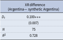

 >