1. Fluid knots and the Jones polynomial
In a series of papers (Liu & Ricca Reference Liu and Ricca2012, Reference Liu, Ricca, Moffatt, Bajer and Kimura2013) we have derived the skein relations of certain knot polynomials, such as the Kauffman bracket, the Alexander–Conway and the Jones polynomial, from the helicity of ideal fluid knots. Most notably, we have introduced the Jones polynomial as a new invariant of topological fluid mechanics (Ricca & Liu Reference Ricca and Liu2014). In the present paper, by relying on these earlier results we extend this approach further, and derive the HOMFLYPT polynomial (Freyd et al. Reference Freyd, Yetter, Hoste, Lickorish, Millett and Ocneanu1985; Przytycki & Traczyk Reference Przytycki and Traczyk1987), which is a two-variable version of the Jones polynomial. Since the HOMFLYPT skein relations are obtained by combining the independent contributions from writhe and twist helicity, we believe that HOMFLYPT provides a more powerful tool to detect topological complexity of fluid structures, such as vortex filaments in classical and quantized turbulence, and magnetic fields in astrophysical flows.
In the last couple of years striking evidence of the existence of knotted structures has been provided by a number of remarkable theoretical and experimental advances, including the mathematical proof of the existence of knotted solutions to Euler equations (Enciso & Peralta-Salas Reference Enciso and Peralta-Salas2012), the construction of knotted solutions to Maxwell equations (Kedia et al. Reference Kedia, Bialynicki-Birula, Peralta-Salas and Irvine2013), and the laboratory production of vortex knots and links in water (Kleckner & Irvine Reference Kleckner and Irvine2013). Meanwhile, overwhelming evidence that vorticity and magnetic fields tend to self-organize into coherent flux tubes and bundles of filaments (Douady, Couder & Brachet Reference Douady, Couder and Brachet1991; Ishihara et al. Reference Ishihara, Kaneda, Yokokawa, Itakura and Uno2007; Mouri, Hori & Kawashimab Reference Mouri, Hori and Kawashimab2007; Baggaley et al. Reference Baggaley, Barenghi, Shukurov and Sergeev2012; Cirtain et al. Reference Cirtain, Golub, Winebarger, De Pontieu, Kobayashi, Moore, Walsh, Korreck, Weber, McCauley, Title, Kuzin and DeForest2013), provides further evidence for possible new relationships between geometric and topological properties of complex fluid systems and energy contents (Barenghi, Ricca & Samuels Reference Barenghi, Ricca and Samuels2001; Moisy & Jiménez Reference Moisy and Jiménez2004; Buck & Simon Reference Buck and Simon2012; Ricca Reference Ricca2013; Kondaurova et al. Reference Kondaurova, L’vov, Pomyalov and Procaccia2014).
To investigate things further, and to fix ideas, let us consider a tangle of vortex filaments in an incompressible ideal fluid. Each vortex filament
 $K$
(of small cross-section) is centred on a closed space curve
 $X$
, of vector position
 $\boldsymbol{X}$
. Vorticity is given by
 ${\bf\omega}=\boldsymbol{{\rm\nabla}}\times \boldsymbol{u}$
, where
 $\boldsymbol{u}$
is the associated velocity field. For a multi-component link
 $L=\cup _{i}K_{i}$
of
 $N$
vortex filaments (possibly knotted), the helicity
 $H=H(L)$
is defined by
 $$\begin{eqnarray}H(L)=\int _{L}\boldsymbol{u}\,\boldsymbol{\cdot }\,{\bf\omega}\,\text{d}^{3}\boldsymbol{x},\end{eqnarray}$$
where integration is done over the total volume of
 $\text{supp}({\bf\omega})$
in
 $L$
. This is a well-known invariant of ideal fluid mechanics, that for thin filaments admits interpretation in terms of linking numbers (Moffatt Reference Moffatt1969; Berger & Field Reference Berger and Field1984; Moffatt & Ricca Reference Moffatt and Ricca1992), i.e.
 $$\begin{eqnarray}H=\mathop{\sum }_{i}SL_{i}\,{\it\Phi}_{i}^{2}+2\mathop{\sum }_{i\neq j}Lk_{ij}{\it\Phi}_{i}{\it\Phi}_{j},\end{eqnarray}$$
where
 $SL_{i}$
denotes the (Călugăreanu–White) self-linking number of
 $X_{i}$
,
 $Lk_{ij}$
is the (Gauss) linking number between
 $X_{i}$
and
 $X_{j}$
, and
 ${\it\Phi}_{i}$
is the
 $i$
th flux (or circulation) of
 ${\bf\omega}$
within each
 $K_{i}$
. For a single thin tubular knot in isolation, (1.1) takes the simple form
 $$\begin{eqnarray}H(K)={\it\Phi}\oint _{K}\boldsymbol{u}\,\boldsymbol{\cdot }\,\text{d}\boldsymbol{l},\end{eqnarray}$$
where
 $\boldsymbol{u}$
is the self-induced velocity given by the Biot–Savart law, and
 $\text{d}\boldsymbol{l}\equiv \hat{\boldsymbol{t}}\,\text{d}s$
the line element along the axis of
 $K$
(where
 $s$
is the arc-length and
 $\hat{\boldsymbol{t}}$
the unit tangent vector to
 $X$
). By making use of a reference ribbon associated with the tubular knot, given by
 $R=R(\boldsymbol{X},\hat{\boldsymbol{N}})$
(where
 $\hat{\boldsymbol{N}}$
is the unit normal vector to
 $X$
),
 $H(K)$
admits decomposition in terms of writhe and twist, according to the Călugăreanu–White theorem (Moffatt & Ricca Reference Moffatt and Ricca1992; Ricca & Moffatt Reference Ricca, Moffatt, Moffatt, Zaslavsky, Comte and Tabor1992):
 $$\begin{eqnarray}H(K)={\it\Phi}^{2}SL={\it\Phi}^{2}(\mathit{Wr}+\mathit{Tw}),\end{eqnarray}$$
where
 $\mathit{Wr}=\mathit{Wr}(X)$
is the writhing number of
 $X$
, and
 $\mathit{Tw}=\mathit{Tw}(R)$
is the total twist number of
 $R$
.
By analysing the knot properties in a standard knot diagram (see, for instance, Kauffman Reference Kauffman1987), and by making use of a plausible statistical hypothesis on the state decomposition of the crossing sites (see Remark 3 at the end of § 3), Liu & Ricca (Reference Liu and Ricca2012) (here below referred to as LR12) proved the following result.
Theorem 1. Let
 $K$
denote a physical knot. If the helicity of
 $K$
is
 $H=H(K)$
, then
 $$\begin{eqnarray}\text{e}^{H(K)}=\text{e}^{\oint _{K}\boldsymbol{u}\,\boldsymbol{\cdot }\,\text{d}\boldsymbol{l}},\end{eqnarray}$$
appropriately re-scaled, satisfies (with a plausible statistical hypothesis) the skein relations of the Jones polynomial
 $V=V_{K}$
.
Remark 1. To make sense of
 $\text{e}^{H(K)}$
,
 $H(K)$
must be written in dimensionless form, by normalizing (1.3) with respect to some reference value of flux.
2. Kauffman’s
 $R$
polynomial and bracket polynomial

In general, a knot polynomial is generated by a set of rules, the so-called skein relations, that prescribe how a ‘state’ of a particular crossing site, represented for example by the over-crossing  in the knot diagram (see, for example, the leftmost diagram of figure 1), is related to its opposite (i.e. the under-crossing
 and the relative ‘smoothing’ given by two parallel strands (the non-crossing
 ). The recursive application of the skein relations to each crossing site allows the computation of the polynomial for a given knot (see the examples of § 4 below). In LR12, as a preliminary step towards the derivation of the Jones skein relations, we derived the skein relations of the so-called Kauffman
 $R$
-polynomial for oriented knots (LR12, see equations (13)–(15)), given by

where, in general,
 $R=R_{K}(k,z)$
is a two-variable polynomial of
 $K$
in terms of the variables
 $k$
and
 $z$
. In LR12 we set
 $z=k-k^{-1}$
, a choice instrumental for the derivation of the Jones polynomial
 $V=V_{K}(z)$
, thus reducing
 $R_{K}$
to the degenerate one-variable form known as the Alexander–Conway polynomial
 $\boldsymbol{{\rm\nabla}}=\boldsymbol{{\rm\nabla}}_{K}(z)$
. In order to derive HOMFLYPT, that is, a two-variable polynomial
 $P=P_{K}(a,z)$
, we must re-examine the derivation of (2.2) and introduce a second, independent relation for the variable
 $a$
. By writing
 $R$
in terms of
 $t^{H(K)}$
(where
 $t$
is a dummy variable in the skein relation, and
 $H$
is non-dimensional), and by using the virtual path decomposition shown in figure 1 for the positive figure-of-eight, we had

where by writing  we implicitly assumed zero contribution from the helicity of the trivial circle, i.e.
 . A similar assumption made for the negative figure-of-eight led to

Since
 $R$
is the regular isotopy version of the HOMFLYPT polynomial, the necessary adjustment must be made by considering the writhe normalization of its regular isotopy counterpart (Kauffman Reference Kauffman1987, Reference Kauffman2001). On the other hand, physical insight for the appropriate correction comes from analysing the third skein relation of the bracket polynomial
 $B_{K}({\it\alpha})=\langle \cdot \rangle$
derived for unoriented knots (see LR12, equation (31)), given by

where the presence of
 $f({\it\alpha})$
, a function of the bracket variable
 ${\it\alpha}$
, suggests a possible contribution from the helicity associated with the circular loop (or any topologically equivalent configuration).
By virtually adding and subtracting local paths (denoted by blue arcs in the online version), a positive crossing can be reduced to a straight segment, a trivial circle and a (positive) figure-of-eight.

3. Derivation of the skein relations of the HOMFLYPT polynomial
Inspired by the helicity decomposition (1.4) in terms of writhe and twist, we can think of the skein relations as independent functions of the writhe and twist contribution, separately (see also Kauffman Reference Kauffman2001, pp. 55–56). Hence, we propose to revise the derivation of the two skein relations for the HOMFLYPT polynomial
 $P=P_{K}(a,z)$
according to the following scheme.
-
(i) Skein relation for the
$z$
-variable: writhe contribution from crossing state information (regular isotopy). -
(ii) Skein relation for the
$a$
-variable: twist contribution from Reidemeister type I move (ambient isotopy).


3.1. Skein relation for the
$z$
-variable: writhe contribution

Let us reconsider the Kauffman bracket skein relations for unoriented knots (LR12, equation (30)), given by

Here  arises from the technique of adding/subtracting imaginary paths (as in figure 1; see also LR12, figure 6), and
 ${\it\lambda}_{1}$
is a parameter that takes into account the uncertainty associated with the writhe value of
 . By endowing the knot strands in (3.1) and (3.2) with orientation, we have

The (inconsistent) term  on the right-hand side of the above equations vanishes by considering the difference between crossing states, that is,

The
 $R$
-polynomial of a knot
 $K$
is readily obtained from its bracket polynomial
 $\langle \cdot \rangle$
by the standard position (Kauffman Reference Kauffman2001)
 $$\begin{eqnarray}R[K]={\it\alpha}^{w}\langle K\rangle ,\end{eqnarray}$$
where
 $w$
is the (directional) writhe of the knot diagram
 $[K]$
. By applying (3.6) to a non-crossing state of
 $[K]$
, we have

By switching the non-crossing state to an over-crossing (or an under-crossing), and by applying (3.6), we have

Hence, by taking the difference between the two states, and by using (3.7), we have

By defining
 $k={\it\alpha}^{2}$
and
 $z=k-k^{-1}$
, one of the skein relations of the
 $R$
polynomial is readily obtained:

The skein relation for the
 $z$
-variable of the HOMFLYPT polynomial is finally derived by the standard position (Kauffman Reference Kauffman2001, pp. 650–651)
 $$\begin{eqnarray}P(a,z)=a^{-w}R(a,z),\end{eqnarray}$$
where
 $a$
will be defined in terms of twist in the following subsection (see (3.17) below). Since

and

we have

3.2. Skein relation for the
$a$
-variable: twist contribution

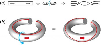
As discussed in earlier works (Moffatt Reference Moffatt1990; Ricca & Moffatt Reference Ricca, Moffatt, Moffatt, Zaslavsky, Comte and Tabor1992), twist insertion by Dehn surgery (see, for example, Adams Reference Adams1999) provides an idealized technique for twist insertion in fluid knots; by using the reference ribbon concept (see figure 2), twist insertion can be realized by a three-step mathematical process given by a virtual cut, rotation and reconnection (in this sequence) performed locally on the knot strand. By using the standard decomposition of helicity in terms of writhe and twist (see (1.4)), Dehn surgery can thus be interpreted as a technique for insertion/deletion of (twist) helicity alternative (and complementary) to the insertion/deletion of helicity provided by the virtual addition/subtraction of imaginary local paths through a change of writhe (as in figure 1).
(a) By using a reference ribbon, twist can be visualized by a local insertion on the straight band. (b) Twist insertion by Dehn surgery on a torus.

By using the ribbon representation of knot strands, we replace the idealized scheme of figure 1 with that of figure 3. Thus, twist insertion/deletion in the unknotted ribbon  gives
 , and contributes to twist helicity, according to the decomposition

Hence, we can replace (2.4) and (2.5) with

where
 $a=t^{{\it\tau}}$
. Thus (2.2) are replaced by

Using (3.11), these correspond to

Following LR12, and by using the same change of variables introduced by Liu & Ricca (Reference Liu, Ricca, Moffatt, Bajer and Kimura2013) (by taking
 $t=e$
), without loss of generality we can set

where
 ${\it\lambda}_{{\it\omega}}$
and
 ${\it\lambda}_{{\it\tau}}$
are two parameters that take into account the uncertainty (or probability) associated with writhe and twist values of some reference configuration (as in figure 7 of LR12).
By using a ribbon representation of knot strands, a (positive) crossing can be virtually decomposed into a straight ribbon and a circular band with (positive) twist.

The skein relations of the HOMFLYPT polynomial for oriented knots are given by (2.1) and (3.14):

where
 $z=k-k^{-1}$
. Thus, we have proved the following result.
Theorem 2. Let
 $K$
denote a physical knot. If the helicity of
 $K$
is
 $H=H(K)$
, then
 $$\begin{eqnarray}\text{e}^{H(K)}=\text{e}^{\oint _{K}\boldsymbol{u}\,\boldsymbol{\cdot }\,\text{d}\boldsymbol{l}},\end{eqnarray}$$
appropriately re-scaled, satisfies (with a plausible statistical hypothesis) the skein relations of the HOMFLYPT polynomial
 $P=P_{K}$
.
Remark 2. To make sense of
 $\text{e}^{H(K)}$
,
 $H(K)$
must be written in dimensionless form, by normalizing (1.3) with respect to some reference value of the field strength.
Remark 3. The derivation of the result above relies on the following statistical hypothesis (instrumental for the derivation of the Kauffman bracket polynomial and the skein relation for the
 $z$
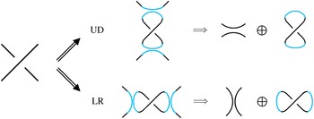
-variable in § 3.1; see LR12, section 4.1): the contribution of the unoriented crossing to the skein relation is computed by assuming a virtual branching process of the crossing, which leads to two independent, equally probable states (represented by the left–right and up–down schemes shown in figure 4). In the absence of specific prescriptions, this is equivalent to the ergodic assumption that all possible (virtual) reconfiguration states of the given knot or link are admissible and equally probable. Particular fluid-mechanical specifications, suggested by the physics of the process, will eventually help to select specific conditions for the most appropriate statistics.
The unoriented crossing on the left can be virtually split by adding and subtracting local paths (denoted by blue arcs in the online version) following the up–down (UD) or the left–right (LR) scheme above. Both decompositions are assumed to contribute equally to the computation in the skein relation.

The skein relations (3.21) and (3.22) generate the HOMFLYPT polynomial
 $P=P_{K}$
. For a link of
 $N$
components, since each knot carries information about its own field strength, and
 $H(K)$
is a diffeomorphic invariant of
 $K$
, then
 $P_{K}$
is a diffeomorphic invariant of knot type and flux. Hence, we have the following corollary.
Corollary 1. The HOMFLYPT polynomial provides a new invariant of ideal fluid mechanics, by extending the dual dependence of helicity on linking number and flux.
4. HOMFLYPT polynomial of some elementary cases
For the purpose of illustration we present explicit calculations of the HOMFLYPT polynomial of some elementary cases. HOMFLYPT polynomials of more complex topologies can be readily computed by some of the knot tabulators available online (such as KnotAtlas). Implementation of the HOMFLYPT skein relations rely on reduction schemes exemplified by the diagrams of figure 5. As well as their mathematical meaning, these diagrams acquire physical significance when the fluid evolution is governed by reduction in topological complexity based on single reconnection events (as discussed in the second example of § 6). As we shall see, reduction schemes can also provide physical intuition for realistic cascade processes in turbulent flows.
Reduction schemes for the Hopf link
 $\boldsymbol{H}_{-}$
and the trefoil knot
 $\boldsymbol{T}^{L}$
.

4.1.
$N$
disjoint, unknotted loops
$\boldsymbol{U}_{N}$


For a single loop the initial condition of the skein relations (3.21) prescribes  ; this can be used to determine the polynomial of two unknotted loops
 $\boldsymbol{U}_{2}$
. By using (3.22), we have

Hence

Similarly for three unknotted loops
 $\boldsymbol{U}_{3}$
, by (3.22), we have

so that

In general, for a disjoint union of
 $N$
oriented, unknotted loops
 $\boldsymbol{U}_{N}$
, we have

Hence

Note that in this case the value of the polynomial does not depend on the relative orientation of the loops.
4.2. Hopf link
For the negative Hopf link
 $\boldsymbol{H}_{-}$
(see figure 5
a), we have

so that
 $$\begin{eqnarray}P(\boldsymbol{H}_{-})=a^{3}z^{-1}-az^{-1}-az.\end{eqnarray}$$
4.3. Left-handed trefoil knot
For the left-handed trefoil knot
 $\boldsymbol{T}^{L}$
(see figure 5
b), we have

so that
 $$\begin{eqnarray}P(\boldsymbol{T}^{L})=2a^{2}+a^{2}z^{2}-a^{4}.\end{eqnarray}$$
5. Quantifying structural complexity by topological information
In this section we present the HOMFLYPT computation of some simple topological cases, highlighting some key features relevant to fluid systems. From a physical viewpoint the HOMFLYPT polynomial
 $P=P_{K}(a,z)$
is not only a new invariant of topological fluid mechanics, but it can take into account the contributions from writhe and twist separately, through the
 $z$
and
 $a$
variables. From this viewpoint it appears to be more powerful than the Jones (and Alexander–Conway) polynomial. Indeed, HOMFLYPT reduces to Jones when we take
 $a={\it\tau}^{-1}$
and
 $k={\it\tau}^{1/2}$
(see LR12, equation (37)); thus, by (3.20), we have
 $$\begin{eqnarray}ak^{2}=\text{e}^{\bar{{\it\tau}}}\text{e}^{2\bar{{\it\omega}}}=1,\end{eqnarray}$$
that is,
 $$\begin{eqnarray}{\it\lambda}_{{\it\tau}}\mathit{Tw}=-4{\it\lambda}_{{\it\omega}}\mathit{Wr},\end{eqnarray}$$
which poses a rather strict constraint on the admissible writhe and twist contributions of the reference mean flow field. We point out that this constraint is absent in the case of HOMFLYPT, where writhe and twist can indeed take any possible real value independently.
For simplicity let us set
 ${\it\Phi}=1$
for all knot types (as in the case of superfluid vortex tangles). The values of
 and
 can be either derived from global helicity measurements based on (1.1), or estimated on the basis of computational/observational data of the flow field (see, for example, Barenghi et al.
Reference Barenghi, Ricca and Samuels2001). Writhe can be directly computed from geometric analysis of the tangle, whereas twist can be obtained as the difference between helicity, given by (1.1), and the sum of (Gauss) linking numbers and writhe, by using (1.2). Hence, the vortex tangle will be identified by HOMFLYPT information (implemented by numerical codes in real-time analysis) computed on the basis of the mean flow field values given by
 $\langle \mathit{Wr}\rangle$
and
 $\langle \mathit{Tw}\rangle$
(and mirror contributions). In the absence of such information (and here for the sake of illustration) we take
 $$\begin{eqnarray}\displaystyle & \langle \mathit{Wr}\rangle ={\textstyle \frac{1}{2}},\quad {\it\lambda}_{{\it\omega}}={\textstyle \frac{1}{2}}\Rightarrow k=\text{e}^{1/2}, & \displaystyle\end{eqnarray}$$
 $$\begin{eqnarray}\displaystyle & \langle \mathit{Tw}\rangle ={\textstyle \frac{1}{2}},\quad {\it\lambda}_{{\it\tau}}={\textstyle \frac{1}{2}}\Rightarrow a=\text{e}^{1/4}. & \displaystyle\end{eqnarray}$$
 $N$
disjoint unlinked, unknotted loops
 $\boldsymbol{U}_{N}$
, the positive Hopf link
 $\boldsymbol{H}_{+}$
, the negative Hopf link
 $\boldsymbol{H}_{-}$
, the left-hand trefoil
 $\boldsymbol{T}^{L}$
, the right-hand trefoil
 $\boldsymbol{T}^{R}$
, the figure-of-eight knot
 $\boldsymbol{F}^{8}$
, the Whitehead link
 $\boldsymbol{W}$
, the mirror image of the Whitehead link
 $\tilde{\boldsymbol{W}}$
, and the Borromean rings
 $\boldsymbol{B}$
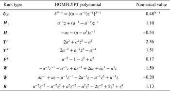
. The corresponding polynomial expressions and their numerical values are shown in the table of figure 6.
Numerical values of the HOMFLYPT polynomial of some elementary knots and links for
 ${\it\Phi}=1$
,
 $k=\text{e}^{1/2}$
,
 $a=\text{e}^{1/4}$
,
 $z=k-k^{-1}$
.
 $\boldsymbol{U}_{N}$
denotes
 $N>1$
disjoint unlinked, unknotted loops,
 $\boldsymbol{H}_{+}$
the positive Hopf link,
 $\boldsymbol{H}_{-}$
the negative Hopf link,
 $\boldsymbol{T}^{L}$
the left-hand trefoil,
 $\boldsymbol{T}^{R}$
the right-hand trefoil,
 $\boldsymbol{F}^{8}$
the figure-of-eight knot,
 $\boldsymbol{W}$
the Whitehead link,
 $\tilde{\boldsymbol{W}}$
the mirror image of the Whitehead link, and
 $\boldsymbol{B}$
the Borromean rings.

Since individual loops are frequently formed in fluid dynamical systems (as a result of physical interaction and reconnection), the case of unlinked, unknotted loops deserves particular interest. From (3.20) and (4.1), we have
 $$\begin{eqnarray}{\it\delta}=\frac{a-a^{-1}}{k-k^{-1}}=\frac{\text{e}^{\bar{{\it\tau}}}-\text{e}^{-\bar{{\it\tau}}}}{\text{e}^{\bar{{\it\omega}}}-\text{e}^{-\bar{{\it\omega}}}}=\frac{\sinh \bar{{\it\tau}}}{\sinh \bar{{\it\omega}}},\end{eqnarray}$$
with
 ${\it\delta}\rightarrow \bar{{\it\tau}}/\bar{{\it\omega}}$
when both
 $\bar{{\it\tau}}$
and
 $\bar{{\it\omega}}$
tend to 0.
In practice, the precise value of
 $a$
,
 $a^{-1}$
,
 $k$
and
 $k^{-1}$
depend on the particular physical context, and marked differences are indeed possible (for instance between vortex and magnetic systems), particularly so as regards the value of
 $a$
and
 $a^{-1}$
. For vortex flows, twist is expected to be consistent with the tube vorticity direction and orientation, and so mainly positive. This means that the probability of having
 $a$
and
 $a^{-1}$
values equi-distributed is very low; hence,
 $a$
and
 $a^{-1}$
should be weighted by numerically different values, say
 ${\it\lambda}_{{\it\tau}^{+}}$
and
 ${\it\lambda}_{{\it\tau}^{-}}$
, with
 $0\leqslant {\it\lambda}_{{\it\tau}^{-}}\ll {\it\lambda}_{{\it\tau}^{+}}\leqslant 1$
. This is not the case for magnetic flux tubes in astrophysical flows, where twist (often of mechanical origin) is not explicitly related to the magnetic field direction (although the polarities of vortical regions are often correlated). There are also physical limits to twist values related to writhe or kink instabilities, for which
 $\mathit{Tw}=O(1)$
. Writhe, on the other hand, does not suffer from such limitations, with no particular constraints on
 ${\it\lambda}_{{\it\omega}^{+}}$
and
 ${\it\lambda}_{{\it\omega}^{-}}$
.
Finally, we would like to mention a remarkable property of HOMFLYPT, which can be exploited by numerical implementation of structural complexity methods. This is summarized by the following set of rules (Lickorish & Millett Reference Lickorish and Millett1988).
Proposition 1.
 $$\begin{eqnarray}\displaystyle & P(L_{1}\,\#\,L_{2})=P(L_{1})P(L_{2}); & \displaystyle\end{eqnarray}$$
 $$\begin{eqnarray}\displaystyle & P(L_{1}\sqcup L_{2})={\it\delta}P(L_{1})P(L_{2}). & \displaystyle\end{eqnarray}$$
In (5.6)
 $L_{1}\,\#\,L_{2}$
denotes the connected sum of any component of the oriented link
 $L_{1}$
with any component of the oriented link
 $L_{2}$
; in (5.7)
 $L_{1}\sqcup L_{2}$
denotes the disjoint union of
 $L_{1}$
and
 $L_{2}$
, assuming that
 $L_{1}$
and
 $L_{2}$
are placed at some distance apart, so that no part of
 $L_{1}$
crosses over or under any part of
 $L_{2}$
. Note that direct application of (5.7) to the case of
 $N$
disjoint loops gives (4.6).
6. New insight into fluid-mechanical behaviour
Numerical implementation of HOMFLYPT provides useful information to gain new insight into fluid-mechanical behaviour of real fluid flows. Here we mention some possible applications that we believe will be helpful for turbulence research.
(i) As experiments and direct numerical simulations of superfluid turbulence show (Tsubota, Araki & Nemirovskii Reference Tsubota, Araki and Nemirovskii2000; Leadbeater et al.
Reference Leadbeater, Samuels, Barenghi and Adams2003; Kondaurova et al.
Reference Kondaurova, L’vov, Pomyalov and Procaccia2014), vortex tangles evolve through continuous production and interaction of small(er)-scale unlinked, unknotted vortex loops. Evidence shows that these loops are planar ring-like structures, with almost no writhe and no twist (superfluid vortices are like empty tubes with no internal structure); thus, their internal helicity is either zero or negligible. Being unlinked to the rest of the system, these loops do not contribute to the total helicity of the system; thus, as far as helicity is concerned, they are like ghost structures. In terms of energy, though, their contribution is not negligible, since they interact dynamically with the rest of the system. Hence, any information on the relationship between helicity, taken as a measure of structural complexity, and energy cannot be accurate enough. Moreover, in cases such as those exemplified by the Whitehead link or the Borromean rings, where the linking number fails to distinguish essential links from unlinked systems, this information gives completely incorrect results. From this viewpoint HOMFLYPT provides not only a more accurate account of the topological complexity of the flow, but it can also distinguish situations where a given number of loops are present (see § 4.1): indeed, being
 $P(\boldsymbol{U}_{N})$
invertible, it can be used to track the precise number
 $N$
of unlinked, unknotted vortex rings present in the fluid. This information, related to energy, can help to establish detailed relationships between topological complexity and energy.
(ii) The recent laboratory experiments on the production and free decay of vortex knots and links in water (Kleckner & Irvine Reference Kleckner and Irvine2013) show that both trefoil knots and Hopf links follow a similar reconnection cascade: the topology gets gradually reduced, with complexity reduced in steps of one crossing lost at each reconnection event, until final dissipation of unlinked, unknotted smaller loops. Remarkably, a similar reconnection pattern (which brings the trefoil knot to the Hopf link, the unknot and the unlink of two smaller unknotted loops) is also shown to characterize DNA recombination: quite remarkably, a mathematically rigorous characterization of the topological mechanism of DNA unlinking is shown to be the only possible pathway that strictly reduces complexity by stepwise unlinking (Shimokawa et al. Reference Shimokawa, Ishihara, Grainge, Sherratt and Vazquez2013). The mathematics behind this proof suggests that it would be equally applicable to flux tube reconnections. In any case, if the change in topology is due to a single reconnection event, the reconnection pattern can be reproduced by following the ‘smoothing’ sequence of the reduction scheme shown in § 4. For example, by combining the schemes of figure 5(b,a) (in this order), we have
 $$\begin{eqnarray}\boldsymbol{T}^{L}{\rightsquigarrow}\boldsymbol{H}_{-}{\rightsquigarrow}\boldsymbol{U}_{1}{\rightsquigarrow}\boldsymbol{U}_{2},\end{eqnarray}$$
where the last step is due to the application of the skein relation to the coiled unknot (because of the presence of the apparent crossing) to produce two smaller rings. By analysing the smoothing process of more complex topologies we can make predictions of typical reconnection cascades. For the Borromean rings, for example, a simple exercise shows that we should expect something like
 $$\begin{eqnarray}\boldsymbol{B}{\rightsquigarrow}\tilde{\boldsymbol{W}}{\rightsquigarrow}\boldsymbol{T}^{R}{\rightsquigarrow}\boldsymbol{H}_{+}{\rightsquigarrow}\boldsymbol{U}_{1}{\rightsquigarrow}\boldsymbol{U}_{2},\end{eqnarray}$$
or
 $$\begin{eqnarray}\boldsymbol{B}{\rightsquigarrow}\boldsymbol{W}{\rightsquigarrow}\boldsymbol{F}^{8}{\rightsquigarrow}\boldsymbol{H}_{-}{\rightsquigarrow}\boldsymbol{U}_{1}{\rightsquigarrow}\boldsymbol{U}_{2},\end{eqnarray}$$
according to whether the first reconnection event takes place in the outer or inner region of
 $\boldsymbol{B}$
. Numerical implementation of these ideas to analyse more complex situations will provide information on preferential decay patterns for structural complexity and energy.
(iii) Direct numerical implementation of software dedicated to topological analysis of fluid structures is readily available. Rob Scharein’s KnotPlot, for example, can analyse data extracted from fluid flow simulations (by tracking vorticity, magnetic field, low pressure, or density regions), and compute the HOMFLYPT polynomial to any degree of accuracy. Similar analyses made on complex tangles of superfluid vortices (Barenghi et al. Reference Barenghi, Ricca and Samuels2001; Kondaurova et al. Reference Kondaurova, L’vov, Pomyalov and Procaccia2014) proved that this can be done rather efficiently. By relating changes in topology and structural complexity to changes in energy, this process can be iterated in real time, so as to have a time-dependent information on adaptive topology by HOMFLYPT implementation. This approach can be used to reveal the presence of hierarchical order, occurrence of generic reconnection pathways and preferential routes to energy dissipation.
7. Conclusions
In this paper we provide a rigorous proof of the derivation of the HOMFLYPT polynomial invariant from the helicity of fluid knots and links (Theorem 2), by deriving the HOMFLYPT skein relations from helicity (§§ 3.1 and 3.2). Since in ideal conditions vortex (or magnetic) lines are transported, with constant flux, by the flow of an ideal fluid, their topology is conserved in time. Hence, our result establishes HOMFLYPT as a new invariant of topological fluid mechanics (Corollary 1). Proof of the derivation of the HOMFLYPT skein relations for the variables
 $a$
and
 $z$
necessary for the polynomial computation is done in two steps: in § 3.1, by interpreting the contribution in the
 $z$
variable in terms of writhe, and in § 3.2, by relating
 $a$
to the twist contribution. The physical interpretation of the skein relations in terms of writhe and twist contributions appears to be new and illuminates the respective role of the skein relation in the HOMFLYPT computation. As illustration, a number of simple cases are considered (§ 4), including the case of a system of
 $N$
disjoint, unknotted loops, the Hopf link and the left-handed trefoil knot, all typical examples of topological structures that are likely to occur in real fluid flows. Moreover, the reduction schemes associated with the skein relations (as shown in the examples of figure 5) seem to provide useful physical intuition for typical reconnection cascade patterns, when topological complexity gets reduced by a single reconnection event. In § 5 we apply HOMFLYPT to the case of a homogeneous tangle of vortex filaments of equal circulation, and we compute numerical values for a number of cases, including the Whitehead link and the Borromean rings, both having linking number zero. Real-time, direct numerical implementation of HOMFLYPT will provide useful information to gain new insight into fluid-mechanical behaviour of real fluid flows. In § 6 we give three examples: (i) the HOMFLYPT ability to detect the presence of zero-linking number structures (such as a system of unlinked vortex rings), that otherwise would escape the helicity count; (ii) the prediction of typical reconnection cascade patterns for structures that evolve by reducing complexity through a single reconnection event, by using the reduction schemes associated with the polynomial skein relations; (iii) the HOMFLYPT flow data analysis by dedicated software (such as KnotPlot) to establish time-dependent relationships between structural complexity, energy transfers and dissipation rates. Implementation of HOMFLYPT as a new diagnostic tool in direct numerical simulations of classical and superfluid turbulent flows might prove useful in determining new connections between energy localization and transfer.
Acknowledgements
We wish to thank the Isaac Newton Institute for Mathematical Sciences for the kind hospitality and support provided during our stay in Cambridge (UK), where part of this work was initiated. We would also like to thank Ken Millett for his comments on a preliminary version of this paper.