2.1. Experimental set-up

All measurements were conducted within a recirculating rectangular flume at Tsinghua University, as illustrated in figure 1(a). The experimental flume is 45 cm in width, 50 cm in height and 20 m in length, with an adjustable slope. The side and bottom walls of the flume are made of transparent glass, providing a clear observation of the flow. Eight ultrasonic level sensors were placed along the flume to monitor water levels (the measurement accuracy of the water level is $\pm$ 0.2 mm). A pump and electromagnetic flowmeter were installed on the backwater pipe to control and monitor the flow rate. To eliminate large-scale structures and flatten the flow, a series of honeycomb panels were installed at the flume entrance. The measurement section was located 13.6 m (approximately 263–567 $h$ ) downstream of the flow entrance, well satisfying the length requirement for achieving fully developed flow conditions (Zampiron et al. Reference Zampiron, Cameron, Stewart, Marusic and Nikora2023). The tailgate was 6.4 m downstream of the measurement section, sufficiently distant to prevent any influence on the measurement section.

Figure 1.

(a) Experimental flume, (b) top view of the measurement section and (c) definition of flow parameters over a rough bed.

Experiments were performed under four steady and uniform flow conditions, with the rough bed configured with regular glass spheres with a diameter ( $D$ ) of 6 mm (see figure 1 b). For fully rough flow over a bed covered with uniform spheres, the equivalent roughness height $k_s$ is calculated from $U^+=({1}/{\kappa })\mathrm{ln}(y/k_s)+B$ , where $B=$ 8.5 is a constant (Ligrani & Moffat Reference Ligrani and Moffat1986). The calculated value of $k_s$ varies from 2.02 to 2.75 as the Reynolds numbers increase. The innerscale normalised equivalent roughness height is defined as $k_s^+=k_s u_\tau /\nu$ . The theoretical bed (where the mean streamwise velocity is zero) was located at 0.15 $D$ below the crests of the spheres (see figure 1 c). As can be seen in table1, the displacement of the theoretical bed level is suggested to be 0.1 $D$ to 0.227 $D$ from the crest of roughness by others (Grass Reference Grass1991; Singh, Sandham & Williams Reference Singh, Sandham and Williams2007; Cameron, Nikora & Stewart Reference Cameron, Nikora and Stewart2017; Mazzuoli & Uhlmann Reference Mazzuoli and Uhlmann2017), thus, the value of 0.15 $D$ adopted in the present study is reasonable. The friction velocity $u_\tau$ is obtained by extending the linear part of the Reynolds shear stress to the theoretical bed level. The $u_{\tau , PG} (=-h\mathrm{d}P/\mathrm{d}S=\rho ghS)$ obtained from streamwise pressure gradient is also calculated. The deviation between $u_\tau$ and $u_{\tau , PG}$ ( $ | u_\tau -u_{\tau , PG} | /u_{\tau , PG}$ ) is less than 3 $\%$ , validating the accuracy of friction velocity in the present study. The investigations were conducted at low relative submergence, with the ratio of water depth to equivalent roughness height ( $h/k_s$ ) ranging from 11.4–18.5. 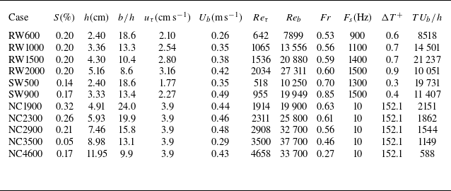The friction Reynolds number $Re_\tau$ of the four flow cases ranges from 642 to 2034, spanning a wide enough range to reveal potential Reynolds number effects. More details of the flow parameters for each case can be seen in table 2 (see cases labelled as RW+ $Re_\tau$ ).

Table 1.

The location of the theoretical bed level below the roughness crest in other studies. Here TBL represents turbulent boundary layer flow; $d$ is the distance from the theoretical bed level to the top of the sphere.

Table 2.

A summary of flow and PIV parameters of smooth- and rough-wall OCF datasets considered in this study. Here $S$ , is channel slope; $h$ , the flow depth which starts from the theoretical bed to the flow surface; $b/h$ , the aspect ratio of the flow; $u_\tau$ and $U_b$ , the friction and depth-averaged velocity; $Re_\tau = u_{\tau } h / \nu$ and $Re_b = {U}h/ \nu$ , the friction and bulk Reynolds numbers; $\nu$ , kinematic viscosity; $ \textit{Fr} = U_b /\sqrt {gh}$ , the Froude number, with $g$ being the gravity acceleration; $F_s$ , sampling frequency; $\Delta T^+$ , innerscale normalised time interval; $T$ , acquisition time duration.

In addition to the rough-wall cases, measurements were conducted in smooth-wall (SW) conditions at two comparable Reynolds numbers, with $Re_{\tau }=$ 518 and 955, denoted as SW500 and SW900, respectively. The two smooth-wall cases have the same water depth or, in other words, the same aspect ratio, with that of rough-wall (RW) cases at comparable Reynolds numbers (i.e. RW600 and RW1000). Then, direct comparisons between these smooth- and rough-wall cases are allowed to reveal the effects of rough elements on the results explicitly.

Time-resolved PIV was adopted for the flow velocity measurement. Hollow glass spheres (Dantec Dynamics, HGS-10) with a density of $\mathrm{1.06} \times \mathrm{10^3\,kg\,m^{-3}}$ and a mean diameter of 10 $\unicode{x03BC}$ m served as tracer particles. The measurement section was illuminated by a 1 mm thick laser sheet generated by a continuous laser (532 nm, 5 W). Particle images were acquired by a high-speed CMOS camera (IDT Y7, 64 GB, 1920 $\times$ 1080 pixels) with high-frequency $F_s$ (inner scale normalised time interval ${\Delta }T^{+} = ({\mathrm{1}}/{F_s})/({\nu }/{u_{\tau }^{\mathrm{2}}}) = {{\Delta }T}/{({\nu }/{u_{\tau }^{\mathrm{2}}})}$ less than 1) and long duration $T$ (during which the main flow moves more than 8000 times water depth $h$ ), ensuring that both small- and large-scale energy-containing turbulent motions were resolved. An in-house image postprocessing software, based on a multipass and multigrid window deformation algorithm similar to that of Scarano (Reference Scarano2001), was employed to obtain the velocity fields. The streamwise size of the particle image is 256 pixels, and the spatial resolution is 360 pixels per cm for all the testing cases. As proposed by Duan et al. (Reference Duan, Chen, Li and Zhong2020), a size of 128 pixels in a streamwise direction is sufficiently large to ensure the resultant statistics. The interrogation window size is 24, 24, 20, 20, 32 and 24 pixels for RW600, RW1000, RW1500, RW2000, SW500 and SW900, respectively. Due to this there is a 50 $\%$ overlap between neighbouring interrogation windows, the innerscale normalised spacing ( $\Delta x^+=\Delta y^+ = \Delta x u_\tau / \nu = \Delta y u_\tau / \nu$ ) between two neighbouring velocity points is 8.61, 10.44, 10.00, 10.96, 9.6 and 9.2 for RW600, RW1000, RW1500, RW2000, SW500 and SW900, respectively. In consideration of the reflections from the particles in the near-wall region, the two-dimensional median filter and Gaussian filter were used to enhance the background and eliminate reflections.

For comparative purposes, table 2 also includes some very recent experimental results of rough-wall OCFs within comparable $Re_\tau$ ranges. The experimental results of rough-wall OCFs from Nikora et al. (Reference Nikora, Stoesser, Cameron, Stewart, Papadopoulos, Ouro, McSherry, Zampiron, Marusic and Falconer2019) (labelled as NC+ $Re_\tau$ ) correspond to runs 31, 32, 33, 29 and 22 of their PIV data sets, respectively. The rough-wall OCF results from Nikora et al. (Reference Nikora, Stoesser, Cameron, Stewart, Papadopoulos, Ouro, McSherry, Zampiron, Marusic and Falconer2019) are primarily used for validating the present rough-wall OCF measurements, while the smooth-wall OCF results are used to highlight the effects of roughness.

2.2. Decomposition method of friction factor

For a steady and zero-pressure gradient flow, the double-averaged conservation equations have been proposed to describe momentum, fluid stress and kinetic energy for both fixed-wall conditions (Nikora et al. Reference Nikora, McEwan, McLean, Coleman, Pokrajac and Walters2007a , Reference Nikora, Stoesser, Cameron, Stewart, Papadopoulos, Ouro, McSherry, Zampiron, Marusic and Falconer2019; Zampiron et al. Reference Zampiron, Cameron, Stewart, Marusic and Nikora2023) and mobile-wall conditions (Nikora et al. Reference Nikora, Ballio, Coleman and Pokrajac2013; Papadopoulos et al. Reference Papadopoulos, Nikora, Cameron, Stewart and Gibbins2019). These equations extend the classical Reynolds decomposition of the instantaneous flow parameter ( $u=\overline {u}+u'$ ) by incorporating spatial averaging ( $\overline {u}=\widetilde {\overline {u}}+\langle {\overline {u}}\rangle$ ) within the wall-parallel layer. The superscript ‘ $'$ ’ denotes velocity fluctuation in the time domain, and the wavey line ‘ $\sim$ ’ denotes velocity fluctuation in the spatial domain, while angle brackets and an overbar denote the spatial average and time average of a given quantity, respectively.

As suggested by Nikora et al. (Reference Nikora, Stoesser, Cameron, Stewart, Papadopoulos, Ouro, McSherry, Zampiron, Marusic and Falconer2019), the decomposition of friction coefficient $C_f$ (normalised mean wall shear stress $\langle \tau _w \rangle$ ) for a steady two-dimensional uniform flow can be expressed as follows:

(2.1) \begin{align} C_f & = \frac {12}{Re_b}\frac {1}{N}+\frac {12}{U_b^2h^2N}\int \limits _{y_0}^{y_{\textit{surf}}}(y_{\textit{surf}}-y)\varphi \big \langle - \overline {u'v'}\big \rangle \mathrm{d}y \nonumber \\ & \quad +\frac {12}{U_b^2h^2N}\int \limits _{y_0}^{y_{\textit{surf}}}(y_{\textit{surf}}-y)\varphi \big \langle - {\widetilde {\overline {u}}}{\cdot }{\widetilde {\overline {v}}}\big \rangle \mathrm{d}y, \end{align}

where $y_c$ denotes the level of the rough crest, and $y_{\textit{surf}}$ denotes the level of flow surface. The expression $\langle - \overline {u'v'}\rangle$ and $\langle - {\widetilde {\overline {u}}}{\cdot }{\widetilde {\overline {v}}}\rangle$ represents the turbulent stress and the dispersive stress, respectively. Here $N$ is a parameter that describes the interaction between the flow and the rough bed. For steady two-dimensional uniform flow, $N=3(L_\tau /h)^2+(L_\varphi /h)^3-(h_m/h)^3$ (Nikora et al. Reference Nikora, Stoesser, Cameron, Stewart, Papadopoulos, Ouro, McSherry, Zampiron, Marusic and Falconer2019). Here $h_m$ represents the maximum flow depth ( $h_m = h$ ). $L_\tau$ represents the ‘drag’ length scale which is defined as the vertical position at which the ‘effective’ drag force acting on the rough bed applies; here, $L_\tau = h$ . Here $L_\varphi$ is the ‘depth-roughness’ length scale, $L_\varphi = (3\int _{y_0}^{y_{\textit{surf}}}(y_{\textit{surf}}-y)^{2} (1-\varphi ){\rm d}y)^{\mathrm{1/3}}$ . Here $\varphi$ denotes spatial porosity, $\varphi =V_f/V_0$ , $V_f$ is the fluid-occupied volume and $V_0$ is the total volume (Nikora et al. Reference Nikora, Goring, McEwan and Griffiths2001). The integrals of the present study were conducted from the crest of the spheres to the water surface $[y_c, y_{\textit{surf}}]$ since no data was obtained in the area below $y_c$ . This has minimal impact on the analysis, given that the omitted portion below $y_c$ represents a negligible percentage of the total $C_f$ .

Here, the three terms on the right-hand side of (2.1) represent the contribution of viscous stress $(C_{f,v})$ , turbulent stress $(C_{f,t})$ and dispersive stress $(C_{f,d})$ , respectively. We have

(2.2) \begin{align}&\quad C_{f,v}=\frac {12}{Re_b}\frac {1}{N}, \end{align}

(2.3) \begin{align}& C_{f,t}=\int _{0}^{1}F_T\mathrm{d}\left(\frac {y}{h} \right), \end{align}

(2.4) \begin{align}& C_{f,d}=\int _{0}^{1}F_D\mathrm{d}\left(\frac {y}{h} \right), \end{align}

where $F_T= - 12 {\varphi }/{(U_b^2N)}(1-y/h)\langle \overline {u'v'}\rangle$ and $F_D=-12 {\varphi }/{(U_b^2N)}(1-y/h)\langle \widetilde {\overline {u}}\cdot \widetilde {\overline {v}}\rangle$ represents the weighted contribution of the Reynolds shear stress and dispersive stress to bed shear stress, respectively. In the present study, $C_{f,v}/C_f$ , $C_{f,t}/C_f$ , $C_{f,d}/C_f$ were adopted to provide relative contributions of viscous stress, turbulent stress and dispersive stress to the mean wall shear stress. Due to the absence of a spanwise velocity component, the dispersive stress was obtained by subtracting the viscous and turbulent terms from the total shear stress, i.e. $C_{f,d}=C_f-C_{f,v}-C_{f,t}$ . This approach was implemented to ensure that the analysis remained unaffected, supported by the reliable data quality established in this study (refer to the PIV uncertainty analysis in Appendix A).

Following the scale decomposition of the turbulent portion of $\langle \tau _w \rangle$ in the smooth turbulent boundary layer and OCF (Deck et al. Reference Deck, Renard, Laraufie and Weiss2014; Duan et al. Reference Duan, Zhong, Wang, Zhang and Li2021), this study also performs a scale decomposition of $C_f$ to quantify the contributions of various turbulent scales to $\langle \tau _w \rangle$ . This is realised by invoking the cospectra of spatially averaged turbulent stress $\langle u'v' \rangle$ , considering only the streamwise flow parameters. The cospectrum of $\langle u'v' \rangle$ at a specific $y$ location can be obtained as follows:

(2.5) \begin{align}&\qquad {\Phi }_{\left \langle u'v' \right \rangle }(y,k_x)=\mathrm{2Re}[S_{\left \langle u'v' \right \rangle }(y,k_x)], \\[-12pt] \nonumber \end{align}

(2.6) \begin{align}& S_{\langle u'v' \rangle }(y,k_x)=c{\mathcal{F}} [ \langle u'(y) \rangle ] {\mathcal{F}}^* [ \langle v'(y) \rangle ], \\[6pt] \nonumber \end{align}

where $c$ is a constant determined by satisfying $\langle u'v' \rangle =\int _{0}^{\infty }{\Phi }_{\langle u'v' \rangle }(k_x)\mathrm{d}k_x$ . The notation $\mathrm{Re}[ ]$ represents taking the real part of a complex number. The symbol $\mathcal{F}$ denotes the Fourier transform and the superscript $^*$ indicates its complex conjugate. It is worth mentioning here that since temporal velocity signals were used, Taylor’s hypothesis was adopted to convert the spectra from the frequency domain into the wavenumber (or wavelength) domain.

Through the above derivation, the spectra of $F_T$ , represented as ${\Phi }_{F_T}$ , can be expressed as

(2.7) \begin{equation} {\Phi }_{F_T}=-\frac {12\varphi }{N} \left(1-\frac {y}{h} \right)\frac {{\Phi }_{\left \langle u'v' \right \rangle }(k_x)}{U_b^2}, \end{equation}

and $F_T=\int _{0}^{\infty } {\Phi }_{F_T}(k_x)\mathrm{d}k_x$ .

Therefore, the turbulence-induced friction factor $C_{f,t}$ is given by

(2.8) \begin{equation} C_{f,t}=\int _{0}^{1} \int _{0}^{\infty } {\Phi }_{F_T}(k_x)\mathrm{d}k_x\mathrm{d} \left(\frac {y}{h} \right), \end{equation}

It is known that ${\Phi }_{F_T}$ is influenced by the $y$ positions and turbulent motion scales. As established in prior research, and given that the spectra are used and presented in logarithmic coordinates regarding the turbulent motion scales, (2.8) can also be expressed as

(2.9) \begin{equation} C_{f,t}=\int _{-\infty }^{\infty } k_x{\Phi }_{C_{f,t}}\mathrm{d}(\mathrm{ln}(k_x)), \end{equation}

where ${\Phi }_{C_{f,t}}(k_x)=\int _{0}^{1} {\Phi }_{F_{T}}(k_x)\mathrm{d(}y/h)$ is the spectra of $C_{f,t}$ (Deck et al. Reference Deck, Renard, Laraufie and Weiss2014; Duan et al. Reference Duan, Zhong, Wang, Zhang and Li2021). By dividing (2.9) with $C_f$ , the scale-decomposed contribution of turbulence-induced stress to $\langle \tau _w \rangle$ is obtained as

(2.10) \begin{equation} {C_{f,t}}/C_f=\int _{-\infty }^{\infty }\frac { k_x{\Phi }_{C_{f,t}}}{C_f} \mathrm{d}(\mathrm{ln}(k_x)). \end{equation}

3.1. Friction factor constituents

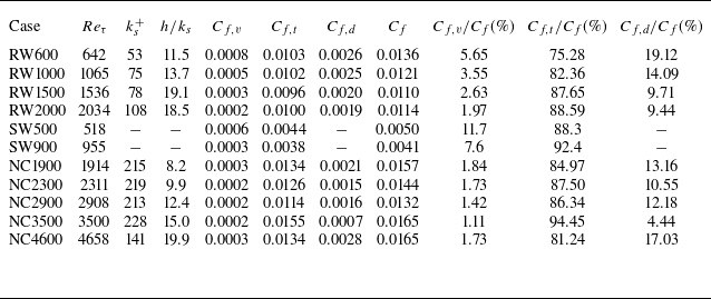
The friction coefficient, denoted as $C_{f}$ along with its constituents, viscous ( $C_{f,v}$ ), turbulent ( $C_{f,t}$ ) and dispersive ( $C_{f,d}$ ), are quantified and delineated in table 3 to provide a comprehensive overview of the components and attributes of the mean wall shear stress $\langle \tau _w \rangle$ . Furthermore, to facilitate comparison, the findings from recent studies on rough-wall OCFs, as described in § 2, are incorporated. Table 3 not only presents the absolute values of these components but also offers their relative values to $C_{f}$ (i.e. $C_{f,v}/C_f$ , $C_{f,t}/C_f$ , $C_{f,d}/C_f$ ), elucidating the contribution percentages of different constituents to $\langle \tau _w \rangle$ .

Table 3.

The friction coefficient and its mechanism-based constituents.

A comparative analysis of rough- and smooth-wall OCFs reveals that in rough-wall OCFs, both $C_f$ and its three components are higher compared with those in smooth-wall OCFs at similar Reynolds numbers. This observation suggests that the presence of roughness in rough-walled flows leads to increased drag forces, which aligns with earlier findings (Kuwata & Kawaguchi Reference Kuwata and Kawaguchi2018). However, due to the presence of supplementary dispersive-induced terms, the relative contributions of viscous stress ( $C_{f,v}/C_f$ ) and turbulent stress ( $C_{f,t}/C_f$ ) are diminished in rough-wall OCFs compared with their counterparts in smooth-wall flows. The results of the present study concerning rough-wall OCFs are consistent with those reported by Nikora et al. (Reference Nikora, Stoesser, Cameron, Stewart, Papadopoulos, Ouro, McSherry, Zampiron, Marusic and Falconer2019) under comparable Reynolds number conditions, thereby validating the measurement accuracy in the present investigation. Further analysis of the three constituents ( $C_{f,v}$ , $C_{f,t}$ , $C_{f,d}$ ) reveals that turbulent stress predominates in influencing the wall-shear stress, accounting for more than 75 % of the total, while viscous stress contributes the least (less than 6 $\%$ ).

Figure 2.

Dependence of the mechanism-based contributions $C_{f,v}/C_f$ , $ C_{f,t}/C_f$ and $C_{f,d}/C_f$ on (a) Reynolds number, (b) relative submergence and (c) innerscale normalised roughness height.

The influence of various parameters, including the Reynolds numbers, relative submergence ( $h/k_s$ ) and innerscale normalised roughness heights ( $k_s ^+$ ), on the three constituents of wall-shear stress ( $C_{f,v}/C_f$ , $ C_{f,t}/C_f$ and $C_{f,d}/C_f$ ) are delineated in figure 2 to elucidate the impact of these parameters on the constituents. Additionally, the rough-wall OCFs results from Nikora et al. (Reference Nikora, Stoesser, Cameron, Stewart, Papadopoulos, Ouro, McSherry, Zampiron, Marusic and Falconer2019) are also incorporated into figure 2 for comparative and validation purposes. Note that their experiments were conducted over rough impermeable beds, while the data sets of the present study were obtained over a permeable rough bed. Nevertheless, the consistency between the results of the present study and those of Nikora et al. (Reference Nikora, Stoesser, Cameron, Stewart, Papadopoulos, Ouro, McSherry, Zampiron, Marusic and Falconer2019) is reinforced by examining the magnitudes and trends of these constituents.

Figure 2 demonstrates distinct dependencies of wall-shear stress constituents on $Re_\tau$ , $h/k_s$ and $k_s ^+$ . In relation to $Re_\tau$ , $C_{f,v}/C_f$ and $C_{f,d}/C_f$ exhibit a decreasing trend while $C_{f,t}/C_f$ demonstrates an increasing trend as $Re_\tau$ increases (refer to figure 2 a). This suggests a reduction in the contributions of viscous and dispersive stress, accompanied by an augmentation in the contribution of turbulent stress to wall shear stress at higher $Re_\tau$ . Similarly, as depicted in figures 2(b) and 2(c), analogous variation trends are observed for the dependency of the three wall-shear stress constituents on $h/k_s$ and $k_s ^+$ , with decreasing trends of $C_{f,v}/C_f$ and $C_{f,d}/C_f$ alongside an increasing trend of $C_{f,t}/C_f$ .

Figure 3.

Wall-normal distribution of (a) $y/h\times F_T/C_f$ and (b) cumulative turbulent contribution to $\langle {\tau _w} \rangle$ , $Cum_T(y)$ . Noting that the $Cum_T(y)$ only takes turbulent contribution into account, thus the integral result is less than 100 % at $y/h = 1$ .

Given the dominant role of turbulent stress in the overall wall-shear stress, a more thorough exploration of this constituent will advance our comprehension of the underlying mechanisms of wall-shear stress. Figure 3(a) presents an initial glimpse of the wall-normal distribution profiles of $y/h\times F_T/C_f$ across the entire water depth, offering insight into contributions of different regions (in wall-normal direction) to the turbulent component of wall-shear stress. Notably, the $y/h\times F_T/C_f$ profiles attain their peak values within the range of $y/h = 0.3-0.4$ for all cases, signifying the most significant local contributions at corresponding wall-normal positions. Comparative analysis of the profiles at varying Reynolds numbers reveals a rising trend with increasing Reynolds numbers, indicating higher local turbulent contributions at larger Reynolds numbers, which is consistent with what has been reported in smooth-wall OCFs (Duan et al. Reference Duan, Zhong, Wang, Zhang and Li2021). Notably, the curves of rough OCFs show great consistency with those of smooth OCFs at $y/h\gt 0.7$ , and they diverged from smooth cases at $y/h\lt 0.7$ . According to previous studies, the roughness sublayer can extend to $3-5k_s$ (Raupach, Antonia & Rajagopalan Reference Raupach, Antonia and Rajagopalan1991; Wu & Christensen Reference Wu and Christensen2010), corresponding to 0.4 $-$ 0.7 $h$ in our study. Therefore, the comparisons between rough and smooth OCFs illustrate that the effects of wall roughness on the turbulent shear stress are confined to the roughness sublayer. The consistency of rough- and smooth-wall OCFs at $y/h\gt 0.7$ aligns with the wall similarity hypothesis. This hypothesis posits that the influence of wall roughness is confined to the roughness sublayer, while turbulent statistics and motions in the outer region remain unaffected (Townsend Reference Townsend1976; Raupach et al. Reference Raupach, Antonia and Rajagopalan1991; Schultz & Flack Reference Schultz and Flack2003; Jiménez Reference Jiménez2004).

Figure 3(b) further shows the cumulative turbulent contribution profiles ( $Cum_T(y)$ ), which were obtained by integrating the area under the profiles of $y/h\times F_T/C_f$ shown in figure 3(a). In the near-wall region, the profiles of $Cum_T(y)$ exhibit a high degree of agreement between different flow cases, followed by a discernible difference in the outer region as $Re_\tau$ increases (higher $Cum_T(y)$ at higher $Re_\tau$ ). It is worth mentioning that the maximum value of $Cum_T(y)$ at $y/h=$ 1 corresponds to the turbulent component $C_{f,t}/C_f$ , which is why it does not reach a value of 100 %. When comparing the $Cum_T(y)$ profiles of present rough-wall OCFs with those of smooth-wall OCFs, it becomes evident that the $Cum_T(y)$ is lower in rough-wall cases. In general, the outer region with $y/h\gt$ 0.2 contributes roughly more than 40 % of the total wall shear stress.

The dependencies of $y/h\times F_T/C_f$ and $Cum_T(y)$ on $h/k_s$ and $k_s ^+$ display similar characteristics (for brevity, not shown herein) to those observed with Reynolds numbers in figure 3, i.e. the maximum values of $y/h\times F_T/C_f$ and $Cum_T(y)$ are increased with the increase of $h/k_s$ and $k_s ^+$ . Since the equivalent roughness height ( $k_s$ ) remains constant for all cases (in the present study), the variation in $Re_\tau$ , $h/k_s$ and $k_s ^+$ primarily reflects changes in water depth or Reynolds numbers. Consequently, the magnitudes of $y/h\times F_T/C_f$ and $Cum_T(y)$ increase with Reynolds numbers.

3.2. Scale decomposition of the ‘turbulent’ stress component

The preceding section (§ 3.1) conducted a thorough analysis of shear stress components and their respective influences on the overall wall-shear stress. This section further explores the role of turbulent motions at different scales in contributing to wall-shear stress. This is achieved by dissecting the turbulent stress component into contributions of various physical length scales, as elucidated in § 2.

Figure 4.

Scale-dependent local contribution $k_x ({y}/{h}){\Phi }_{F_{T} }$ to $\langle {\tau _w} \rangle$ . Innerscale and outerscale normalised coordinates are used in (a–d) and (e–h), respectively. Panels (a–e), (b–f), (c–g) and (d–h) correspond to the results of different cases with the case name labelled in the lower-left-hand corner of each panel. The maximum value is indicated by a white cross symbol.

In figure 4, the scale-dependent local turbulent contributions to the wall-shear stress $\langle \tau _w \rangle$ , denoted as $k_x ({y}/{h}){\Phi }_{F{_T}}/C_f$ , are first presented to examine the impact of different scale motions at various ( $y$ ) positions on $\langle \tau _w \rangle$ . Figures 4 (a–d) and 4(e–h) utilise the inner ( $\lambda _x^+=\lambda _x u_\tau /\nu$ , $y^+=y u_\tau /\nu$ ) and outer scale ( $\lambda _x$ , $y/h$ ) normalised coordinates, respectively, to investigate potential inner/outer scaling laws. Figures 4(a–e), 4(b–f), 4(c–g) and 4(d–h) represent different cases at various Reynolds numbers. Notably, in the innerscale normalised coordinates (figure 4 a–d), significant shifts of peak values are evident along both $y^+$ and $\lambda _x^+$ directions. This is evident from the shift in the position of the white cross symbol in figure 4(a–d) representing the maximum value of $k_x ({y}/{h}){\Phi }_{F{_T}}/C_f$ . Conversely, in the outerscale normalised coordinates (figure 4 e–h), the maximum value of $k_x ({y}/{h}){\Phi }_{F{_T}}/C_f$ corresponds roughly to the same streamwise wavelength $\lambda _x/h$ . These observations suggest that the local turbulent contributions to $\langle \tau _w \rangle$ adhere to the outer scaling, consistent with findings in smooth-wall OCFs (Duan et al. Reference Duan, Zhong, Wang, Zhang and Li2021).

Regarding the wavelengths corresponding to the peak values of $k_x ({y}/{h}){\Phi }_{F{_T}}/C_f$ , two distinct peaks could be consistently identified at $\lambda _{x} = h$ –2 $h$ and $\lambda _{x}=O(10h)$ , respectively. This implies the presence of two dominant turbulent modes contributing to $\langle \tau _{w} \rangle$ . Remarkably, these wavelengths align with well-documented scales of LSMs and VLSMs (Kim & Adrian Reference Kim and Adrian1999; Hommema & Adrian Reference Hommema and Adrian2003; Guala, Hommema & Adrian Reference Guala, Hommema and Adrian2006; Cameron et al. Reference Cameron, Nikora and Stewart2017; Duan et al. Reference Duan, Chen, Li and Zhong2020; Peruzzi et al. Reference Peruzzi, Poggi, Ridolfi and Manes2020; Yao, Chen & Hussain Reference Yao, Chen and Hussain2022). Furthermore, as for the wall-normal positions, the maximum values of $k_x ({y}/{h}){\Phi }_{F{_T}}/C_f$ are universally located at $y/h = 0.3-0.4$ , consistent with earlier observations in figure 3. The alignment of outer normalised wavelengths and $y$ positions of $k_x ({y}/{h}){\Phi }_{F{_T}}/C_f$ peak values in present rough-wall OCFs with those in smooth-wall OCFs (Duan et al. Reference Duan, Zhong, Wang, Zhang and Li2021) support the wall similarity hypothesis.

Figure 5.

Contribution $k_x {\Phi }_{C_{f,t}}/C_f$ of physical length scales to $\langle {\tau _w} \rangle$ , the innerscale and outerscale normalisations are presented in (a) and (b), respectively. The solid and dashed curves represent the results of rough and smooth OCFs.

The investigation proceeded with a comprehensive integration of the position-dependent and scale-dependent local contribution $k_x ({y}/{h}){\Phi }_{F{_T}}/C_f$ across the entire water depth to examine the contribution of different scales to $\langle \tau _w \rangle$ . This integration, represented in the logarithmic coordinate of length scales, takes the form $k_x {\Phi }_{C_{f,t}}/C_f$ . The resulting curves of $k_x {\Phi }_{C_{f,t}}/C_f$ are depicted in figure 5, with inner and outer normalised streamwise wavelengths $\lambda _{x}^+$ and $\lambda _{x}/h$ in figures 5(a) and 5(b), respectively. By comparing the curve characteristics in figures 5(a) and 5(b) with those in figure 4, the outer scaling of turbulent contribution to $\langle \tau _w \rangle$ becomes more evident. In figure 5(a), there are noticeable shifts of the two prominent peaks with $\lambda _{x}^+$ , whereas in figure 5(b), the peaks do not shift with $\lambda _{x}/h$ , and they consistently occur at $\lambda _{x} = 1$ $\sim$ 2 $h$ and $O(10h)$ , respectively, corresponding to LSMs and VLSMs. Additionally, another notable feature observed in figure 5 is the variation in curve magnitude with $Re_\tau$ . Within the short-wavelength ranges, the magnitude of $k_x {\Phi }_{C_{f,t}}/C_f$ decreases as $Re_\tau$ increases, indicating reduced contributions of small scales at higher Reynolds numbers. The $k_x {\Phi }_{C_{f,t}}/C_f$ curves of smooth OCF are higher and demonstrate a larger contribution from turbulent stress. Nevertheless, the observed trends of $k_x {\Phi }_{C_{f,t}}/C_f$ show great consistency in smooth and rough OCFs, further substantiating the dominance of outer region contributions and the similarities between smooth- and rough-wall flows in the outer region.

The difference in skin friction coefficient ( $C_f$ ) between smooth and rough surfaces results in $k_x {\Phi }_{C_{f,t}}/C_f$ being consistently larger for smooth surfaces than for rough ones. It is impractical to directly investigate how the various scales of motion change in a rough bed compared with a smooth one. Therefore, we substitute $C_f$ with $C_{f,t}$ in $k_x {\Phi }_{C_{f,t}}/C_f$ to analyse the impact of different motion scales on $C_{f,t}$ and to discern the variations between smooth and rough surfaces. To reveal these quantitative differences, the $k_x {\Phi }_{C_{f,t}}/C_{f,t}$ curves of rough and smooth-rough OCFs at comparable Reynolds numbers are contrasted in figure 6. The rough-wall cases are depicted with solid lines, while the smooth-wall cases are represented by dashed lines. To highlight the differences between the two flow types, the areas between the curves are shaded, with red and blue regions representing higher and lower value regions in rough-wall OCFs, respectively. Figures 6(a–b), 6(c–d) and 6(e–f) correspond to comparisons of $k_x {\Phi }_{C_{f,t}}/C_{f,t}$ , the $uv$ cospectra and $uu$ spectra at different Reynolds numbers, respectively.

Figure 6.

Comparison of $k_x {\Phi }_{C_{f,t}}/C_{f,t}$ , $uv$ cospectra and $uu$ spectra between rough and smooth OCFs at comparable Reynolds numbers. The curves at each higher position are added by a constant marked on the left-hand side. The $uv$ cospectra and $uu$ spectra are extracted at $y/h\lt$ 0.2 to emphasise the difference between the two flows in the near-wall region.

As depicted in figure 6(a,b), the curves of $k_x {\Phi }_{C_{f,t}}/C_{f,t}$ for rough-wall OCFs are higher than those of smooth-wall OCFs in the small wavelength ranges ( $\lambda _x \lt h$ ), while the curves of rough-wall OCFs turn to be lower than those for smooth-wall OCF cases in the larger wavelength ranges ( $\lambda _x \gt h$ ). This indicates that the contributions from turbulent motions at $\lambda _x \lt h$ and $\lambda _x \gt h$ in rough-wall OCFs are lower and higher, respectively, than those in smooth-wall OCFs. Similar characteristics are also observed in comparisons between the $uv$ cospectra (see figure 6 c,d), which further verified the accuracy of the measurements in the present study. To the best of our knowledge, this is the first time that the features of wall-shear stress in rough-wall OCFs have been reported from the perspective of scale decomposition and compared with those of smooth-wall OCFs. Similar conclusions are reported by Barros & Christensen (Reference Barros and Christensen2019) as they pointed out that roughness significantly alters the distribution of Reynolds shear stress as a function of scale. In their study, the lower wavenumber (or higher wavelengths) Reynolds shear stress content shifts towards shorter streamwise wavelengths along the low-momentum path (Barros & Christensen Reference Barros and Christensen2019). Compared with smooth-wall flow, most Reynolds shear stress content resides at scales comparable to roughness.

We now delve into the underlying mechanisms that explain the reduced contributions of large-scale structures to turbulent wall-shear stress observed in rough-wall OCFs compared with smooth-wall OCFs. As proposed by Zampiron, Cameron & Nikora (Reference Zampiron, Cameron and Nikora2020), the presence of secondary currents can inhibit the development of VLSM and affect the bed friction in OCF. They concluded that the friction factor may increase if depth-scale secondary currents are present or decrease under conditions of subdepth-scale secondary currents and suppressed VLSMs. This means the decreases in contribution from VLSMs to $\langle {\tau _w} \rangle$ can be attributed to the VLSMs suppression by small-scale secondary currents induced by the rough wall. Besides, as proposed by Ma et al. (Reference Ma, Xu, Sung and Huang2023), the strength of small-scale wall detached motions ( $ly^+\lt 100$ , which are also regarded as small-scale secondary currents in their study) is increased in the near-wall region of rough channel flows. As noted by Anderson et al. (Reference Anderson, Barros, Christensen and Awasthi2015), secondary currents are sustained by roughness-induced spanwise heterogeneities in the Reynolds stress, leading to an imbalance between the production and dissipation of turbulent kinetic energy. Those secondary currents are most pronounced in the roughness sublayer, and the reduction in Reynolds shear stress within VLSMs can be attributed to these secondary currents (Barros & Christensen Reference Barros and Christensen2019).

Indeed, the strength of $uu$ spectra and $uv$ cospectra in figure 6(c,d) are decreased in rough OCFs, especially in the larger wavelength ranges. Since the turbulent component of wall shear stress is determined by integrating the Reynolds shear stress, the observed decrease in the contribution of VLSMs to $ \langle \tau _w \rangle$ might be the by-product caused by small-scale secondary currents in the near wall region.

3.3. Contributions from different scale ranges

Integrating the scale-dependent turbulent contribution to $\langle {\tau _w}\rangle$ , as detailed in § 3.2, provides an overview of the cumulative contributions stemming from various turbulent motions across different scales (denoted as $Cum_T (\lambda _x)$ ). The resulting $Cum_T (\lambda _x)$ curves are shown in figure 7, with innerscale and outerscale normalised $\lambda _x$ represented in figures 7(a) and 7(b), respectively. It is noteworthy that, similar to the $Cum_T (y)$ discussed in § 3.1, the maximum values of $Cum_T (\lambda _x)$ correspond to the total turbulent contribution, which remains below 100 %.

In figure 7(a), the $Cum_T (\lambda _x)$ curves exhibit a clear global shift towards larger $\lambda _x^+$ as $Re_\tau$ increases, indicative of heightened contributions from large-scale turbulent motions. Conversely, when the $Cum_T (\lambda _x)$ curves are plotted against outerscale normalised wavelength $\lambda _x/h$ , no discernible shifting along the wavelength direction is observed (refer to figure 7 b), implying that $Cum_T (\lambda _x)$ scales in outer units. The greater magnitude of the $Cum_T (\lambda _x)$ curve at higher $Re_\tau$ values signifies stronger contributions from the corresponding scale ranges to the wall-shear stress. The value of $Cum_T (\lambda _x)$ is higher in smooth OCFs.

Figure 7.

Distribution of cumulative turbulent contribution of physical scales to $\langle {\tau _w} \rangle$ , $Cum_T (\lambda _x )$ , in the innerscale and outerscale normalised wavelength range, respectively.

Given the early revelation of the significance of LSMs and VLSMs (collectively referred to as large-scale turbulent motions) and their disparity in strength between rough- and smooth-wall OCFs, it is imperative to examine their quantitative impact on $\langle {\tau _w} \rangle$ within the current rough-wall OCF context and to elucidate their distinctions from smooth-wall OCFs. To extract the contributions of LSMs and VLSMs to $\langle {\tau _w} \rangle$ , we initially adopt the dividing wavelength $\lambda _x = 3h$ as a cutoff wavelength in $Cum_T (\lambda _x)$ , following the traditions of dividing scales for large-scale turbulent motions within OCF research community.

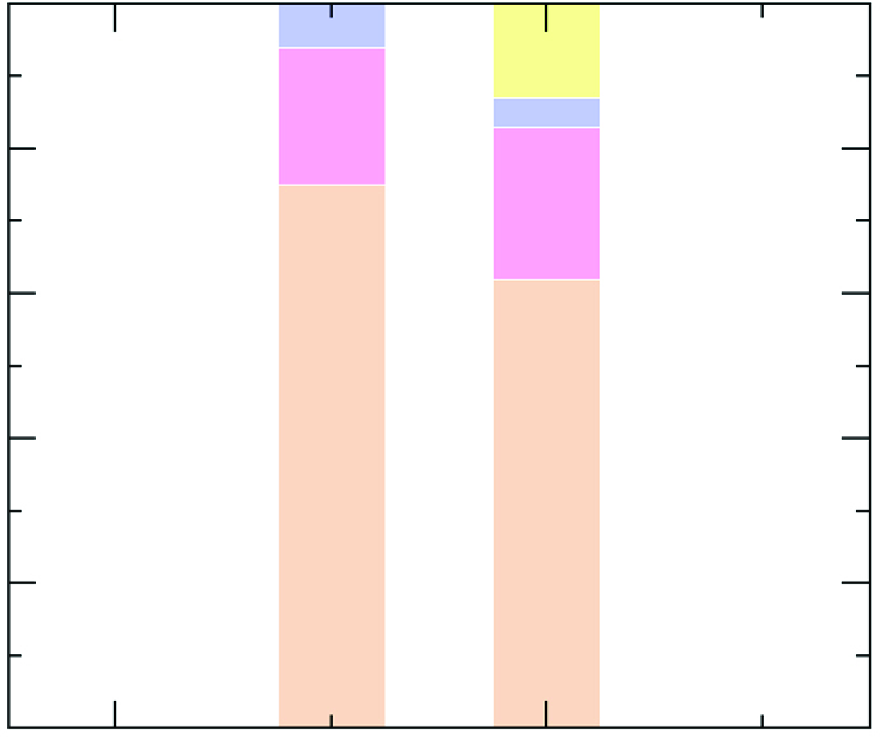
The obtained contributions of LSMs and VLSMs are presented in figure 8, where the results of rough-wall OCFs are shown in figure 8(a), and comparisons between smooth- and rough-wall OCFs at different comparable Reynolds numbers are shown in figures 8(b) and 8(c). For completeness, the contributions from the remaining scale range (namely $\lambda _x \lt 3h$ ), dispersive, and viscous portions are also included in figure 8.

Figure 8.

Contributions of different scale ranges of turbulent motions to $\langle {\tau _w} \rangle$ by adopting the cutoff wavelength of $\lambda _x=3h$ at different Reynolds numbers. (a) The results of rough wall cases, (b,c) comparisons between rough and smooth wall cases at comparable $Re_\tau$ .

Figure 9.

Contributions of different scale ranges of turbulent motions to $\langle {\tau _w} \rangle$ by adopting the cutoff wavelength of $\lambda _x=10h$ at different Reynolds numbers. (a) the results of rough wall cases, (b,c) comparisons between rough and smooth wall cases at comparable $Re_\tau$ .

As can be seen from figure 8(a), the contributions of turbulent motions at $\lambda _x \gt 3h$ increase from 40 % to 44 % as $Re_\tau$ varies from 600 to 2000. Comparisons between rough- and smooth-wall OCFs, as shown in figures 8(b) and 8(c), reveal that the contributions from turbulent motions with $\lambda _x \lt 3h$ and $\lambda _x \gt 3h$ in rough-wall OCFs are both lower than those in smooth-wall OCFs, indicating that the overall turbulent contribution portion of $\langle {\tau _w} \rangle$ is reduced in rough-wall OCFs. The trends of contributions from LSMs and VLSMs with Reynolds number highlight the vital role of this parameter on the strength of LSMs and VLSMs in rough-wall OCFs. Moreover, an even larger cutoff wavelength of $\lambda _x =10h$ , roughly corresponding to the typical length scales of VLSMs, is employed to quantify the contribution of VLSMs to the overall wall-shear stress. The results are depicted in figure 9, analogous to figure 8. As revealed in figure 9(a), the contribution from VLSMs with $\lambda _x \gt 10h$ increases from 18 % to 30 % as the Reynolds number increases.

Therefore, within the range of the Reynolds number considered in the present study, it can be concluded that turbulent motion with $\lambda _x\gt 3h$ and $\lambda _x\gt 10h$ contribute more than 40 % and 18 % of the overall wall-shear stress, respectively. Moreover, the contribution of VLSMs in rough-wall OCFs is lower than that in smooth-wall OCFs, and the contribution of VLSMs to turbulent components $C_{f,t}$ is also lower in rough OCFs than in their smooth counterparts.