2 Measuring Congruence

Scholars studying congruence are often interested in measuring the similarity between elite positions and mass preferences across samples. In some applications—like tests of the median voter theorem—doing so may be fairly simple, and existing measures may be adequate. But scholars often want to compare elite and voter distributions. Since these distributions are represented in Euclidean space, similarity is simply a measure of distance: more similar objects are physically closer to each other. But distance is defined contextually. Research in fields such as graph theory, pattern recognition, cryptography, and molecular biology have developed a staggering array of distance measures for particular applications (Deza and Deza Reference Deza and Deza2006). Choosing among these measures should be of central concern to congruence scholars; as we will show, the choice of measure has important substantive implications.

To begin, let us define a distance $\mathbb{D}$ as a numerical description of how far apart objects are in a metric space, which is defined as an ordered pair ( ${\mathcal{M}},{\mathcal{D}}$ ). ${\mathcal{M}}$ is a set, while ${\mathcal{D}}$ is a metric, a function that defines the distance between objects in the set, i.e., ${\mathcal{D}}:{\mathcal{M}}\times {\mathcal{M}}\rightarrow \mathbb{R}$ .Footnote ⁴ A metric must satisfy nonnegativity, symmetry, Euclid’s triangle inequality, and the identity of indiscernibles.Footnote ⁵ All distances between all elements of ${\mathcal{M}}$ must be identified.

Throughout the paper, we consider the distance between two random variables $X$ and $Y$ . The observed data are events drawn from $X$ and $Y$ , $P_{x}=\{p_{x}(x_{1}),\ldots ,p_{x}(x_{m})\}$ and $P_{y}=\{p_{y}(y_{1}),\ldots ,p_{y}(y_{n})\}$ , respectively. The $x_{i}$ and $y_{j}$ form sequences over the metric space $({\mathcal{M}},{\mathcal{D}})$ , and the $p_{x}(x_{i})$ and $p_{y}(y_{j})$ form the sequences’ associated weights in $P_{x}$ and $P_{y}$ . Define the total weights (or simply “size”) of each sequence such that $W_{x}=\sum _{i}p_{x}(x_{i})$ and $W_{y}=\sum _{j}p_{y}(y_{j})$ . Sets such as $P_{x}$ and $P_{y}$ are known as signatures in the image-retrieval literature, and can be viewed as generalized histograms. Note that since $X$ and $Y$ are random variables, $P_{x}$ and $P_{y}$ are their distributions in $\mathbb{R}^{q}$ , respectively (Levina and Bickel Reference Levina and Bickel2001).

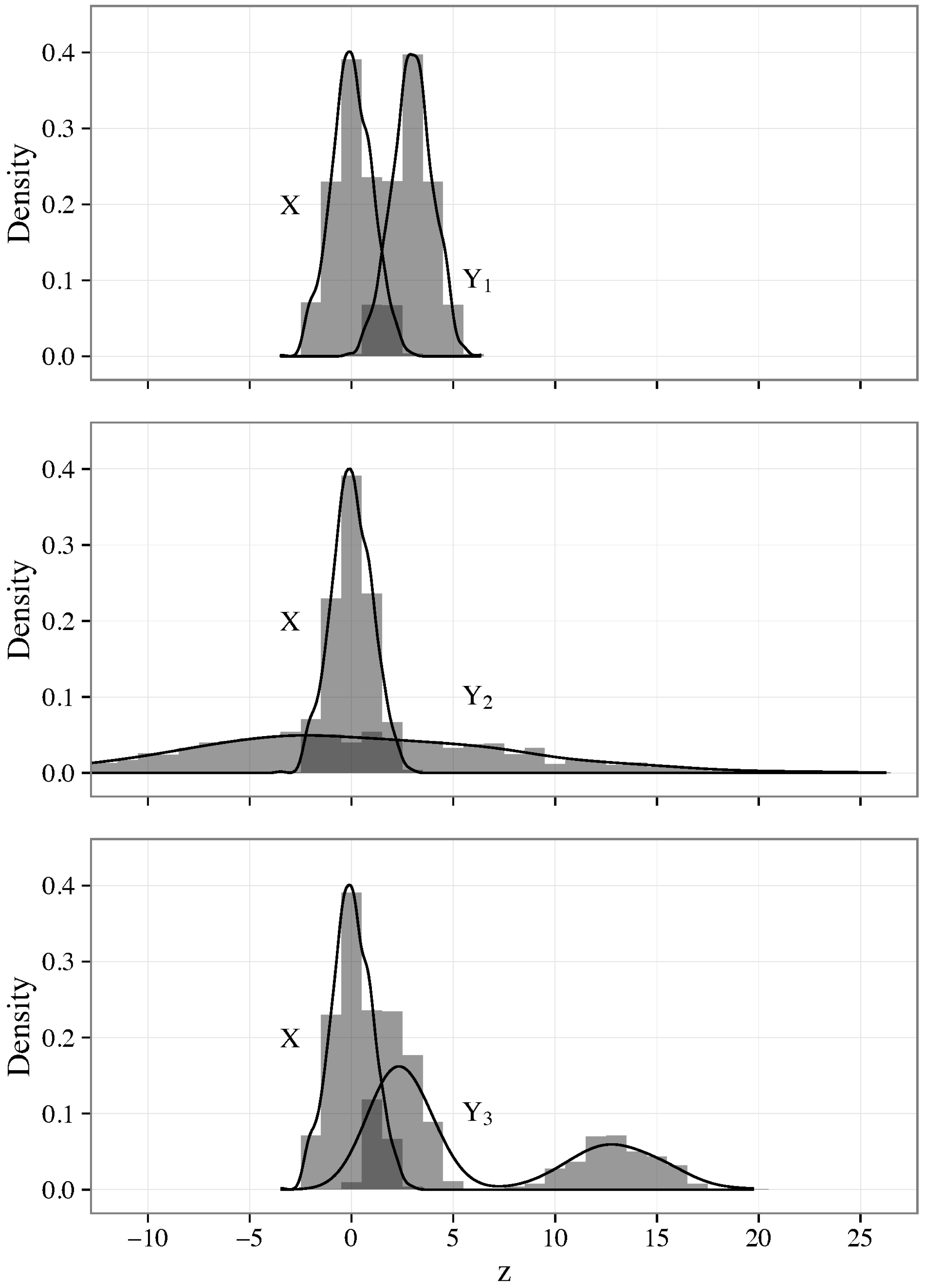
Consider the examples in Figure 1. Each panel plots the empirical histogram and PDF of 1,000 draws from a random variable $X$ that follows a standard-normal distribution in one dimension ( $q=1$ ). The top, middle, and bottom panels also plot these statistics for 1,000 draws each from random variables $Y_{1}$ , $Y_{2}$ , and $Y_{3}$ , respectively, where $Y_{1}\sim {\mathcal{N}}(3,1)$ , $Y_{2}\sim {\mathcal{N}}(0,64)$ , and $Y_{3}\sim \text{Mix}(\unicode[STIX]{x1D706}{\mathcal{N}}(2.5,1),(1-\unicode[STIX]{x1D706}){\mathcal{N}}(13.1,2))$ . Here, $\text{Mix}$ represents a mixture distribution, with mixing weight $\unicode[STIX]{x1D706}=.65$ . We highlight the overlap between histograms in dark gray.

Figure 1.

Three comparisons using simulated data. Three hypothetical distributional comparisons. A good measure of distance should at least indicate that the distributions in the top panel are the most similar.

What attributes are desirable when evaluating a measure of distance? One minimal requirement is ordinality: if $X$ and $Y_{1}$ are closer together than are $X$ and $Y_{2}$ , then our distance function should always return $\mathbb{D}(X,Y_{1})<\mathbb{D}(X,Y_{2})$ . In other words, a good measure of distance ought to at least recover the rank ordering of distributions’ similarity. We also prefer a measure that preserves cardinality, though we consider this a second-order concern. If we know that $Y_{2}$ is twice as far from $X$ as is $Y_{1}$ , we prefer a measure that recovers $\mathbb{D}(X,Y_{1})=2\mathbb{D}(X,Y_{2})$ .Footnote ⁶ Finally, a good measure of distance should use all of the data across the relevant distributions.

The examples in Figure 1 highlight that these properties should hold whether distance is increasing because of differences across sample means or across sample variances. For instance, it is clear from visual inspection that $\mathbb{E}[Y_{3}]>\mathbb{E}[Y_{1}]$ , so we would like a measure that does not report the samples in the bottom panel as more similar than those of the top panel. It is also clear that $\mathbb{V}[Y_{2}]>\mathbb{V}[Y_{1}]$ , so we prefer a measure that reflects this. A good measure of distance should indicate that the distributions in the top panel of Figure 1 are the most similar.

3 Existing Measures

Three measures of congruence are especially popular in political science applications. The first is the simple difference in means, where the distance between $X$ and $Y$ is defined as

(1) $$\begin{eqnarray}\mathbb{D}_{\text{M}}=|\mathbb{E}[X]-\mathbb{E}[Y]|.\end{eqnarray}$$

Here a larger distance indicates less similarity and thus less congruence.

The second is a measure that instead attempts to measure overlap between distributions. Golder and Stramski (Reference Golder and Stramski2010) suggest computing the nonoverlap of empirical cumulative distribution functions (CDFs) for $X$ and $Y$ ,

(2) $$\begin{eqnarray}\mathbb{D}_{\text{CDF}}=\mathop{\sum }_{z\in Z}|[{\mathcal{F}}_{x}(z)-{\mathcal{F}}_{y}(z)]|,\end{eqnarray}$$

where $Z$ is a set of points, chosen by the researcher, at which to evaluate the functions (generally covering the theoretical bounds or values observed in $P_{x}$ and $P_{y}$ ). Other scholars instead use empirical probability density function (PDF) overlap since it is constrained to the unit interval, making regression estimates equivalent to effect magnitudes in percentage points (Andeweg Reference Andeweg, Rosema, Denters and Aarts2011; Lupu and Warner Reference Lupu, Warner, Joignant, Morales and Fuentes2017). This distance, also known as the Bhattacharyya coefficient, is computed as

(3) $$\begin{eqnarray}\mathbb{D}_{\text{PDF}}=\mathop{\sum }_{z\in Z}\min \{f_{x}(z),f_{y}(z)\}.\end{eqnarray}$$

Unlike $\mathbb{D}_{\text{M}}$ and $\mathbb{D}_{\text{CDF}}$ , larger values for $\mathbb{D}_{\text{PDF}}$ indicate distributions that are closer together, and therefore more similar.

All of these measures discard information in the data. As the name “difference-in-means” signals, $\mathbb{D}_{\text{M}}$ is computed by taking expectations over $X$ and $Y$ separately, and then finding the absolute difference between them. This method ignores substantial variation within each distribution. While such reduced summaries may be appropriate for other applications, this approach is too coarse to serve as a default measure of congruence.

Understanding the limitations of overlap measures requires closer attention to quantization, the process of restricting a continuous quantity to discrete values. While we would like to study the similarity between $X$ and $Y$ directly, our only information about these random variables is encoded in the sequences $P_{x}$ and $P_{y}$ . The problem for overlap measures is knowing which elements of these sequences to compare: which events should enter into the distance calculation, and how? In practice, overlap measures solve this problem by binning each set of observations into histograms. This transformation creates a shared index which identifies data that are considered to be “in the same place.” Formally, a histogram of a sequence $P_{x}$ , $\mathbf{H}_{x}=\{h_{x}^{i}\}$ , is a mapping from a set of $q$ -dimensional integer vectors $\boldsymbol{\unicode[STIX]{x1D714}}_{x}$ to $\mathbb{R}^{+}$ . A histogram partitions the underlying space—here, the support of the probability distribution for $P_{x}$ —into a fixed number of hyper-rectangular blocks known as “bins,” centered at the points in $\boldsymbol{\unicode[STIX]{x1D714}}_{x}$ , with $h_{x}^{\unicode[STIX]{x1D714}}$ the number of elements that have a value in the interval indexed by $\boldsymbol{\unicode[STIX]{x1D714}}_{x}$ (Rubner et al. Reference Rubner, Tomasi and Guibas2000). Where $q=1$ , $\boldsymbol{\unicode[STIX]{x1D714}}_{x}$ is a vector, the number of bins is equal to the length of $\boldsymbol{\unicode[STIX]{x1D714}}_{x}$ , and the bins are simply two-dimensional intervals. Allow $\mathbf{H}_{y}=\{h_{y}^{j}\}$ to be defined similarly for the set $P_{y}$ . In practice, $\mathbb{D}_{\text{CDF}}$ and $\mathbb{D}_{\text{PDF}}$ sum overlap among each bin in $\mathbf{H}_{x}$ and $\mathbf{H}_{y}$ , rather than the observed data $P_{x}$ and $P_{y}$ (or the random variables $X$ and $Y$ from which they are drawn).Footnote ⁷

This quantization requires scholars to make decisions about which variation in the data to ignore. Specifically, since overlap measures directly compare bins to their individual counterparts across histograms, $\mathbf{H}_{x}$ and $\mathbf{H}_{y}$ must be of a fixed size, and they must share an index. This constraint forces scholars to choose a single quantization for both distributions $P_{x}$ and $P_{y}$ (and any other distributions they wish to compare), with an identical range and bin width. Data that are naturally quantized—for example, variables which only take integer values—may be amenable to such techniques. However, for continuous variables, there is no rubric for making an objective decision about appropriate quantization.Footnote ⁸ Overlap measures are extremely sensitive to this choice. If the data are quantized too finely, many bins will be empty, driving overlap downward. If they are quantized too coarsely, then important information about the shape of the distributions will be lost as disparate data are grouped together, increasing overlap. In the extreme, for any $X$ and $Y$ , it is possible to construct bin widths such that PDF overlap takes any value on the unit interval (CDF overlap is similarly manipulable).

Even where the data are naturally quantized and share a common index, overlap measures throw out information. That is because overlap measures only compare bins that have the same index across histograms. Put formally, they compute common mass between $h_{x}^{i}$ and $h_{y}^{i}$ , but not $h_{x}^{i}$ and $h_{y}^{j}~\forall i\neq j$ . This means that data from $\mathbf{H}_{x}$ that lie in bins beyond the index in $\mathbf{H}_{y}$ (and vice versa) are ignored. For example, if $X$ and $Y$ are one-dimensional and all observed data are integers, the elements of $P_{x}$ will form a natural index such as $\boldsymbol{\unicode[STIX]{x1D714}}_{x}=\{-3,-2,\ldots ,3\}$ . In that case, all data in $P_{y}$ that fall outside the interval $[-3,3]$ will be effectively discarded in computing overlap.Footnote ⁹ In some sense, this is precisely what overlap measures set out to accomplish: any bins lacking overlap do not contribute to the measure of congruence. Yet, in this example, congruence will be identical whether $Y$ has a local maximum at $12$ or at $10^{12}$ : since both locations fall outside the range of data observed in $P_{x}$ , overlap will always be zero. An empty bin in $\mathbf{H}_{x}$ generates zero overlap, irrespective of how many observations lie in the corresponding bin in $\mathbf{H}_{y}$ . By ignoring the amount and location of all data that do not overlap, these measures force scholars to overlook potentially important information about $X$ and $Y$ .

Overlap measures suffer from one final shortcoming. While it is possible to extend them to multidimensional space, the problems associated with quantization become even worse as more variables are studied simultaneously. Density concentrates near the surface of high-dimensional distributions, increasing the likelihood of empty bins —the curse of dimensionality (Bellman Reference Bellman2010). Moreover, cross-dimensional correlations and multimodality, which are also likely to increase when scholars use multiple survey responses to capture the same latent dimension, exacerbate this problem. Thus, extending overlap measures to multiple dimensions only frustrates the problems associated with them, making congruence even harder to measure reliably.

4 The Earth Mover’s Distance

To address the limitations associated with existing measures of congruence, we propose the EMD. The EMD between $X$ and $Y$ is defined by the solution to a linear optimization problem, the optimal “flow” $f_{ij}^{\ast }$ for moving the distance between $P_{x}$ and $P_{y}$ . Our goal is to minimize $\sum _{i=1}^{m}\sum _{j=1}^{n}f_{ij}d_{ij}$ subject to

(4) $$\begin{eqnarray}\displaystyle f_{ij} & {\geqslant} & \displaystyle 0\quad \text{for }1\leqslant i\leqslant m,1\leqslant j\leqslant n,\end{eqnarray}$$

(5) $$\begin{eqnarray}\displaystyle \mathop{\sum }_{j=1}^{n}f_{ij} & {\leqslant} & \displaystyle p_{x}(x_{i})\quad \text{for }1\leqslant i\leqslant m,\end{eqnarray}$$

(6) $$\begin{eqnarray}\displaystyle \mathop{\sum }_{i=1}^{m}f_{ij} & {\leqslant} & \displaystyle p_{y}(y_{j})\quad \text{for }1\leqslant j\leqslant n,\text{ and}\end{eqnarray}$$

(7) $$\begin{eqnarray}\displaystyle \mathop{\sum }_{i=1}^{m}\mathop{\sum }_{j=1}^{n}f_{ij} & = & \displaystyle \min \left(\mathop{\sum }_{i=1}^{m}p_{x}(x_{i}),\mathop{\sum }_{j=1}^{n}p_{y}(y_{j})\right),\end{eqnarray}$$

where $d_{ij}$ is some description of similarity between the $i$ th and $j$ th elements of the signatures $P_{x}$ and $P_{y}$ , respectively. Together, these pairwise descriptions form the ground distance matrix $\{d_{ij}\}$ , defined by some metric ${\mathcal{D}}(x_{i},y_{j})$ . Once the optimal flow is found, the EMD is defined as

(8) $$\begin{eqnarray}\mathbb{D}_{\text{EMD}}=\frac{\mathop{\sum }_{i=1}^{m}\mathop{\sum }_{j=1}^{n}f_{ij}^{\ast }d_{ij}}{\mathop{\sum }_{i=1}^{m}\mathop{\sum }_{j=1}^{n}f_{ij}^{\ast }},\end{eqnarray}$$

where the denominator is simply a normalization for cases where signatures differ in magnitude.Footnote ¹⁰ Larger values of $\mathbb{D}_{\text{EMD}}$ indicate greater distance, less similarity, and less congruence.

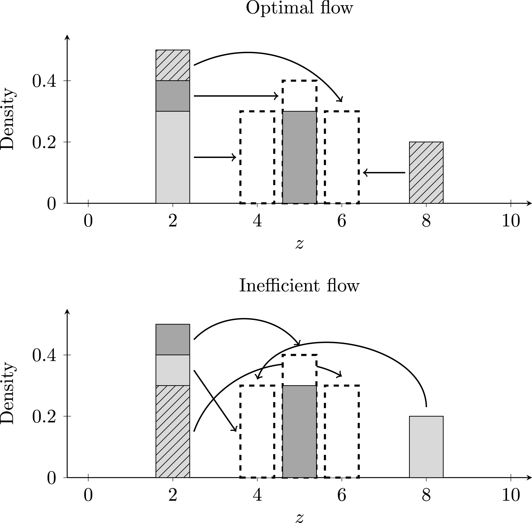
This definition is easier to understand with a simple example. Suppose we want to compute the EMD between two samples of respondents’ self-placement on a 0–10 scale, $P_{x}=\{(2,.5),(5,.3),(8,.2)\}$ and $P_{y}=\{(4,.3),(5,.4),(6,.3)\}$ , where each element in parentheses refers to a location and a density. We want to find the flow that minimizes the amount of “work” (or the “cost”) of moving data such that the signatures are identical. Each panel in Figure 2 presents a different way of moving $P_{x}$ , plotted in various grays, to the location of $P_{y}$ , in dashed lines. One option, the “optimal flow” in the top panel, is to move from left to right, transferring data in $P_{x}$ to the nearest data in $P_{y}$ .Footnote ¹¹ For instance, we start by moving data in $P_{x}$ at $z=2$ to $z=4$ until the total mass there is 0.3, as in $P_{y}$ —generating work of 0.6. Continuing this process yields total work equal to

$$\begin{eqnarray}(|4-2|)(0.3)+(|5-5|)(0.3)+(|5-2|)(0.1)+(|6-2|)(0.1)+(|6-8|)(0.2)=1.7.\end{eqnarray}$$

The constraint in Equation 4 ensures that all data movement counts toward the total work (flow cannot be negative); conditions 5 and 6 require that we cannot move more data than exist at any location (flow cannot exceed the density); and condition 7 ensures that all of the data are moved (the densities sum to 1) (Rubner et al. Reference Rubner, Tomasi and Guibas2000).

Figure 2.

Two examples of “flow.” $P_{x}$ is in gray, while $P_{y}$ is represented in dashed lines. Data plotted in light gray “ends up” at $z=4$ , dark gray at $z=5$ , and stripes at $z=6$ . In the top panel, data in $P_{x}$ are moved to the nearest position available, yielding total work of 1.7. In the bottom panel, a less efficient flow yields more work (2.5). The EMD finds the optimal flow that minimizes work.

Other flows achieve the same result, but may generate more work. The bottom panel displays an “inefficient flow” whereby we move data in $P_{x}$ to a more distant location in $P_{y}$ , yielding total work of 2.5. With more data, and as the set of feasible values $\{z\}$ increases, the number of possible flows grows dramatically. The EMD simply uses the one that minimizes total work. In this example, since the first flow is optimal, the EMD is $\frac{(1)(1.7)}{1}=1.7$ .

This example assumes that the ground distance matrix is defined by the $L_{1}$ norm. This metric, also known as the city-block or Manhattan distance, is given by

(9) $$\begin{eqnarray}{\mathcal{D}}_{L_{1}}(\mathbf{a},\mathbf{b})=\Vert \mathbf{a}-\mathbf{b}\Vert =\mathop{\sum }_{r\in q}|a_{r}-b_{r}|,\end{eqnarray}$$

where $\mathbf{a}$ and $\mathbf{b}$ are points in $q$ -dimensional space.Footnote ¹² The EMD can take any metric, and although this choice is generally dependent on the application (Wang and Guibas Reference Wang, Guibas, Fitzgibbon, Lazebnik, Perona, Sato and Schmid2012), we recommend the $L_{1}$ norm for ease of interpretability. In the foregoing example—as in all one-dimensional calculations—the $L_{1}$ yields an average distance on the scale of the original response. To see this, observe that the maximum we could calculate for a question on a 0–10 scale would be if one sample was entirely located at 0, and the other entirely at 10, yielding $(|10-0|)(1)=10$ . Unlike other metrics, this property also holds for multidimensional comparisons (i.e., $q>1$ ) where the underlying scales are identical. For instance, if we compare three dimensions, all on the same 0–10 scale, then an EMD of 6 can be directly interpreted as the average sum of three-dimensional differences. Further, if the differences between distributions are relatively evenly spread across dimensions, then we could say that the distributions are, on average, 2 points away on each of the original 11-point scales. And if instead of three ordinal scales we have a series of binary questions, then the EMD- $L_{1}$ across all of them is simply a measure of the average number of questions on which respondents differ.

Although the EMD is suitable for measuring distance between any objects in metric space, it is especially useful for problems like the example above, which are most familiar to congruence scholars: computing the cost of transforming one statistical distribution into another. Recall that the signatures $P_{x}$ and $P_{y}$ are sequences of events (“observations”), or empirical distributions drawn from random variables $X$ and $Y$ . If we assume that each has finite $p$ th moments, then the flow $\{f_{ij}\}$ is equivalent to the joint distribution ${\mathcal{F}}(X,Y)$ . Moreover, the signatures’ weights are simply $W_{x}=W_{y}=1$ , so the constraints in Equations (5)–(6) must hold with equality, while Equation (7) and the denominator in Equation (8) both equal 1 (Levina and Bickel Reference Levina and Bickel2001). With the $L_{1}$ norm, we then have the EMD for $P_{x}$ and $P_{y}$ as the minimum sum of simple pairwise distances:

(10) $$\begin{eqnarray}\mathbb{D}_{\text{EMD}}=\mathop{\sum }_{i=1}^{m}\mathop{\sum }_{j=1}^{n}f_{ij}^{\ast }\Vert x_{i}-y_{j}\Vert ,\end{eqnarray}$$

which we can equivalently express as $\mathbb{D}_{\text{EMD}}=\min \{(\mathbb{E}_{{\mathcal{F}}}\Vert X-Y\Vert )\}$ .

Written this way, the EMD appears similar to the measures of congruence that political scientists regularly employ. However, while the mathematical distinctions are subtle, the EMD differs substantially from existing measures. First, the EMD can be used to calculate distances between histograms which need not cover the same range or share an index. More importantly, we need not even use histograms: the EMD can compute distances directly from the data. We simply define each signature as the observations in each sample, weighted by their respective sample sizes so that $W_{x}=W_{y}=1$ , and then calculate pairwise distances between all data points.

The EMD also outperforms overlap measures even when the data are naturally quantized into bins $x_{i}$ and $y_{j}$ . As is evident in Equation 8, the EMD incorporates all pairwise distances between these bins—it calculates distance between $h_{x}^{i}$ and $h_{y}^{j}~\forall i,j$ . Unlike overlap measures, which treat all nonoverlap as equal, the EMD avoids ignoring local maxima and information in the tails of $X$ and $Y$ . The amount and location of data always matter for the EMD.

In one dimension, the EMD also subsumes other definitions of congruence. For instance, suppose $P_{x}$ is a sample of citizens within a particular district, and $P_{y}$ is the (single) representative for that district, so that $P_{y}=p_{y}(y)$ and $p_{y}=W_{y}=1.$ It is clear from Equation 10 that, in this case, the EMD reduces to the total absolute ideological distance between $P_{x}$ and $P_{y}$ . If we were to divide through by $m$ (in this example, the size of the citizen sample), the resulting quantity would be identical to what Golder and Stramski (Reference Golder and Stramski2010) call absolute citizen congruence. Similarly, if we also restrict $P_{x}$ to a single respondent, $x$ , then the EMD reduces to simple absolute distance, $\Vert x-y\Vert$ ; if $x$ is the median voter in a district, then we get what Golder and Stramski (Reference Golder and Stramski2010) term absolute median citizen congruence. Similarly, their relative citizen congruence can easily be recovered from EMD calculations. Thus, depending on how the signatures of interest are defined, the EMD can be employed to measure many conceptualizations of congruence.

The EMD has an important final advantage: it is easily extended to comparing distributions in high dimension.Footnote ¹³ This allows scholars to study congruence across a range of questions, preferences, or issue areas with a single summary statistic. The EMD generalizes directly to multiple dimensions, and since all $d_{ij}$ contribute to total distance, increasing the number of empty bins does not affect the total distance computed. The cost of adding variables is only computation time.Footnote ¹⁴

Scholars should ensure that the multidimensional EMD is appropriate for their application with minimal data processing. We recommend that the variables entering into a multidimensional congruence calculation have similar scales. Each variable in a high-dimensional congruence calculation is weighted equally by default. However, if this is inappropriate for a particular application, scholars can change this by simply including particular variables multiple times in the data. The EMD affords substantial flexibility in constructing a single measure of multidimensional congruence.

5 Simulation Evidence

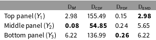
Simulated data illustrate the superior performance of the EMD relative to existing measures. Table 1 reports the measure of congruence for each panel in Figure 1, comparing existing methods with the EMD. As the Table makes clear, the EMD produces better results than do existing measures. In this simulation, the EMD determines that $Y_{1}$ , in the top panel of Figure 1, is closest to $X$ . In contrast, difference-in-means calculations suggest that the most similar distributions are $X$ and $Y_{2}$ , in the middle panel. In fact, they are considered nearly identical, since their empirical means differ only by 0.08, compared to approximately 3 and 6 in the top and bottom panels, respectively. Yet it is clear from visual inspection that this does not capture significant variation in $Y_{2}$ , giving a false impression of similarity. This result follows directly from the definition: recall that $\mathbb{D}_{\text{M}}$ is computed by taking expectations over the marginal distributions of $X$ and $Y$ and then finding the absolute difference between them. As expected, ignoring within-sample variance overstates congruence in this case.

Table 1.

Comparing measures of distance.

Cells report the values that each measure of congruence generates for each of the panels in Figure 1. For each measure, the most similar pair of distributions is bolded.

The EMD also outperforms overlap measures. $\mathbb{D}_{\text{PDF}}$ determines that the $X$ - $Y_{3}$ pairing, in the bottom panel, is the most similar. Yet, again, this is a misleading conclusion: while roughly two-thirds of the data in $Y_{3}$ appear to be very close to that of $X$ , another third is substantially distant. Meanwhile, the similar distributions in the top panel fare the worst. Perhaps most disconcerting, the overlap measures do not agree on the ordering of each distribution’s similarity to $X$ , with $\mathbb{D}_{\text{CDF}}$ favoring the $X$ - $Y_{2}$ pairing in the middle panel. Since both $\mathbb{D}_{\text{PDF}}$ and $\mathbb{D}_{\text{CDF}}$ measure overlap and the PDF is just the first difference of the CDF, we would expect that they produce similar results. Here, not only do they disagree on which distributions are most similar, they also disagree on the relative magnitudes of the distances between distributions. According to CDF overlap, $Y_{2}$ is decisively the closest distribution to $X$ , with the next closest ( $Y_{3}$ ) being 2.5 times farther away. In contrast, according to PDF overlap, the standout is the top panel, with $Y_{1}$ ’s overlap less than 65 percent of $Y_{2}$ ’s.

Finally, it is worth noting that the EMD returns a distance identical to difference-in-means calculations for the top and bottom panels. This is an intuitive result given the construction of these distributions: $Y_{1}$ is equivalent to a secular shift in $X$ of magnitude three, while $Y_{3}$ is essentially an average of two shifts in $X$ , adjusted for the mixing weight $\unicode[STIX]{x1D706}$ . Encouragingly, when two samples are drawn from distributions that are essentially identical in shape, the EMD recovers the true distance in their locations—even when those shifts are embedded as components of more complex mixture distributions.

These encouraging results hold more generally. We conduct a Monte Carlo experiment to investigate each measure’s performance in recovering the ordinality and cardinality of distance comparisons. First, we generate a target sample ( $T$ ) with 100 draws from ${\mathcal{N}}(0,1)$ . Then we randomly generate 1,000 means ( $y_{1},y_{2},\ldots ,y_{1000}$ ), and draw 100 samples from each ${\mathcal{N}}(y_{i},1)$ . Since each of these samples differs from $T$ only in location, the distance between them should be very close to their difference in means: $|y_{i}-0|$ , or just $|y_{i}|$ . We then generate 1,000 variances ( $z_{1},z_{2},\ldots ,z_{1000}$ ) and draw 100 samples from each ${\mathcal{N}}(0,z_{i})$ . Here, distance should be increasing in the true difference in variances, $|z_{i}-1|$ , since each sample has the same mean as $T$ .Footnote ¹⁵ Finally, we calculate each of these 2,000 distances using the three existing measures and the EMD.Footnote ¹⁶

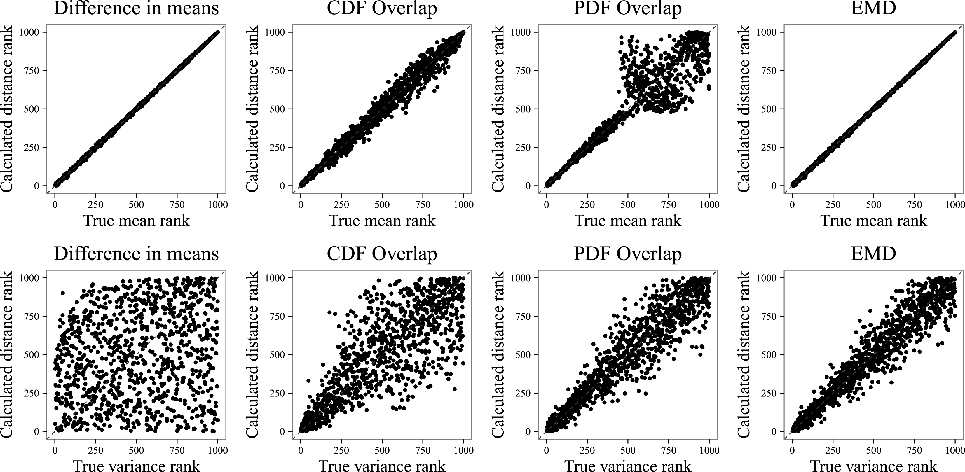
Preserving ordinality is our primary concern. We expect that comparing the orderings of the $|y_{i}|$ ( $|z_{i}-1|$ ) and the distance calculations should yield a one-to-one correspondence: samples with larger differences in means (differences in variances) should be considered farther away from the target sample. For that reason, Figure 3 plots the ranked means (top row) and variances (bottom row) against the ranked calculated distances. Root mean squared error (RMSE) calculations—the mean difference between a sample’s actual rank and its distance rank—are presented in Columns 2 and 3 of Table 2.

Figure 3.

Monte Carlo simulations of measures of congruence: ordinality. We compare the rank order of computed distances between a “target” sample and 1,000 samples with randomly generated means (top row) and 1,000 samples with randomly generated variances (bottom row). We expect a good measure of congruence to preserve ordinality: it should return a one-to-one correspondence between the ranked differences in means (variances) and the ranked computed distance. See the online appendix for the (very similar) cardinality results.

Table 2.

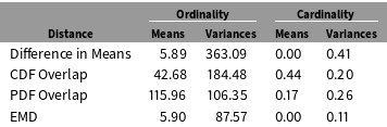
RMSE for Monte Carlo simulations.

Root mean squared error for each measure of congruence across 2,000 simulations. Note that the scale is 1 to 1,000 for ordinality but 0 to 1 for cardinality.

As with the examples in Figure 1, the EMD outperforms existing measures. Both the EMD and difference in means have a neat correspondence between the ranked distances and the real $|y_{i}|$ ordering, with an average error of about 0.6%. In contrast, while CDF overlap does not appear to suffer from any systematic bias, it struggles to recover ordinality, with an RMSE eight times larger than the EMD. PDF overlap’s difficulty recovering a rank ordering in the top row highlights the problem of very little overlap. For the larger half of $|y_{i}|$ , the results become essentially random, as PDF overlap is zero, and $\mathbb{D}_{\text{PDF}}$ is unable to tell how far apart the samples are. Moving to the bottom row, the EMD continues to recover ordinality, although with more difficulty. RMSE in the rank-ordering variances rises to about 9%, but this is a substantial improvement over any of the other measures. Thus, the most important rubric by which to judge a measure of distance—its ability to preserve ordinality—provides clear evidence that we should favor the EMD.

To examine cardinality, we scale the means, variances, and distances computed to the unit interval and compare their (linear) correspondence. The results look similar. Columns 4 and 5 in Table 2 indicate that the EMD is increasing perfectly in the true difference in means between samples, and errs by approximately 11% in the true difference in variances. Both of these substantially outperform the other measures. These results provide clues as to why overlap measures produce such different conclusions about congruence using the same data: they are largely unable to recover accurate descriptions of distributions’ similarity. Across all of these 2,000 samples, the EMD best preserves both ordinality and cardinality of distance comparisons.Footnote ¹⁷

6 Empirical Applications

There are good theoretical reasons to think that the EMD is a better measure of congruence than those currently employed in political science. We have also demonstrated its advantages using simulated data. How might adopting the EMD affect empirical results of substantive interest to political scientists?

We answer these questions with regard to two debates in the study of mass–elite congruence. The first centers on whether electoral rules affect the degree of congruence between voters and their elected officials. Scholars within this debate ask whether proportional electoral systems offer higher levels of mass–elite congruence than do majoritarian systems. A second debate regards whether party system institutionalization and socioeconomic factors positively correlate with congruence in Latin America. Since we lack an empirical benchmark for measuring true congruence, we do not intend for these applications to further demonstrate the advantages of the EMD. Rather, we use them to show that adopting the EMD significantly changes how we answer these important substantive questions.

6.1 Electoral rules and ideological congruence

Scholars of representation have become interested in the degree of congruence between citizens’ preferences and policymakers’ ideological positions (Powell Reference Powell2006, Reference Powell2000). At the most basic level, these studies have shown that mass–elite congruence varies across space and time—that is, that some governments more closely reflect the preferences of the citizenry than others (Dalton Reference Dalton1985; Miller and Stokes Reference Miller and Stokes1963). One possible reason for this cross-national variation is that some political institutions produce more congruent governments than others. In particular, an “ideological congruence controversy” (Powell Reference Powell2009) has emerged regarding the role of electoral systems in promoting mass–elite congruence on left–right ideology. The scholarly debate is between those who find that electoral systems of proportional representation generate more mass–elite ideological congruence than majoritarian electoral systems (Huber and Powell Reference Huber and Powell1994; Powell and Vanberg Reference Powell and Vanberg2000; McDonald and Budge Reference McDonald and Budge2005; Powell Reference Powell2006, Reference Powell2009; Ezrow Reference Ezrow2007; Budge and McDonald Reference Budge and McDonald2007) and those who find little or no difference across electoral systems (Blais and Bodet Reference Blais and Bodet2006; Golder and Lloyd Reference Golder and Lloyd2014; Ferland Reference Ferland2016). Yet, as Powell (Reference Powell2009) demonstrates, scholars engaging in these empirical debates use different sets of data covering different time periods. Most importantly for our purposes, they also employ different measures of congruence.

One prominent example is an analysis by Golder and Stramski (Reference Golder and Stramski2010) of data from the parliamentary systems included in the Comparative Study of Electoral Systems (CSES). At the time they conducted their analysis, there were 37 election studies in the CSES from parliamentary systems with the necessary variables. They covered 22 countries during the period 1996–2005. Today, the CSES includes 81 surveys from 33 parliamentary systems that have the necessary variables, covering the period 1996–2013.Footnote ¹⁸

The CSES surveys ask respondents to place themselves on a 0–10 left–right ideological scale. They also ask them to place up to nine political parties on the same scale. Golder and Stramski (Reference Golder and Stramski2010) use the average placement of each party by the 40 percent most educated respondents as a measure of the party’s ideological position.Footnote ¹⁹ Using the share of seats obtained by each party in the lower legislative chamber, they construct an ideological distribution of legislators. They then use the CDF overlap measure to compare the ideological distribution of survey respondents and the ideological distribution of legislators. Most importantly, they compare CDF overlap among majoritarian and PR electoral systems, finding that legislatures in PR systems are significantly more congruent with mass ideology than are majoritarian systems.Footnote ²⁰

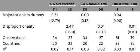
Columns 1 and 2 of Table 3 replicate the analysis of electoral rules and ideological congruence that Golder and Stramski (Reference Golder and Stramski2010) report.Footnote ²¹ Like these authors, we find a positive, but statistically insignificant relationship between electoral rules and CDF overlap when we use a dummy for majoritarianism. However, when we regress CDF overlap on a continuous measure of disproportionality, the positive association reaches statistical significance. For Golder and Stramski (Reference Golder and Stramski2010, 104), this result offers, “strong evidence that countries with PR electoral rules are more likely to have legislatures that are congruent with the ideological preferences of the citizenry than countries with majoritarian ones.”

Table 3.

Electoral rules and ideological congruence.

Sources: Bormann and Golder (Reference Bormann and Golder2013); CSES; Gandrud (Reference Gandrud2015); Golder and Stramski (Reference Golder and Stramski2010). Notes: OLS estimates. Positive values mean less congruence. The dependent variable in (1) and (2) is CDF overlap, as calculated by Golder and Stramski (Reference Golder and Stramski2010, “G & S”). $^{\ast }\text{p}<0.05$ .

In columns 3 and 4 of Table 3, we use the same set of CSES cases, the same data transformations, and the same quantization, but now measure congruence using the EMD. In other words, the only difference with the analysis in columns 1 and 2 is that we apply the EMD optimization equation rather than calculating CDF overlap. Regardless of whether we measure majoritarianism dichotomously or continuously, our results now reveal no statistically significant relationship between congruence and electoral rules, and our estimates suggest a substantively small effect at best.

Given that the CSES has expanded dramatically since Golder and Stramski (Reference Golder and Stramski2010) conducted their analysis, we also updated their dataset to see if additional data points reveal any relationships. In columns 5 and 6 of Table 3, we recalculate the EMD on the full sample of parliamentary elections now available in the CSES. In keeping with Golder and Stramski’s approach, we employed Gandrud’s (Reference Gandrud2015) continuous measure of disproportionality and constructed a majoritarianism dummy variable based on how each country is coded in Bormann and Golder’s (Reference Bormann and Golder2013) database of electoral systems.Footnote ²² And we limited our sample of mass respondents to educated citizens by dropping those who did not complete high school. Finally, since our updated sample includes a number of observations within the same country over time, we cluster our standard errors by country (see Golder and Lloyd Reference Golder and Lloyd2014).Footnote ²³

With the EMD and an expanded dataset, we still find no relationship between electoral rules and mass–elite congruence. Regardless of whether we use a majoritarianism dummy variable or a continuous measure of disproportionality, we never find evidence for the theory that PR systems better represent citizen preferences. At best, our estimates suggest a substantively minuscule effect of electoral rules that sometimes runs in the opposite direction. When we replace the problematic CDF overlap measure of congruence with the EMD, we find no convincing evidence that legislatures in PR systems better reflect the ideological preferences of citizens.

6.2 Mass–elite congruence in Latin America

Debates about congruence among parliamentary systems have revolved primarily around electoral rules. Scholars of the developing world instead point to other factors to explain why democracies in these contexts seem to poorly represent voter preferences. In Latin America, scholars regularly cite presidential policy switches (Stokes Reference Stokes2001; Lupu Reference Lupu2016), institutions that centralize power in the executive (O’Donnell Reference O’Donnell1994), weak and uninstitutionalized party systems (Mainwaring and Scully Reference Mainwaring and Scully1995), widespread clientelism (Calvo and Murillo Reference Calvo and Murillo2013), low levels of development, and high economic inequality. Only recently have studies emerged that test these claims by comparing mass–elite congruence across countries and over time.

These studies use a wide variety of measures of congruence for different subsets of countries in the region, making their findings difficult to compare directly. But a substantial number find that mass–elite congruence correlates with more institutionalized party systems (Luna and Zechmeister Reference Luna and Zechmeister2005; Kitschelt et al. Reference Kitschelt, Hawkins, Luna, Rosas and Zechmeister2010; Bornschier Reference Bornschier2013; Otero Felipe and Rodríguez Zepeda Reference Otero Felipe and Rodríguez Zepeda2014). Several studies also find a positive relationship between economic prosperity and congruence (Luna and Zechmeister Reference Luna and Zechmeister2005; Selios Reference Selios2015).

Part of the interest in studying mass–elite congruence in Latin America is the unique set of data available for the region. Since the mid-1990s, the University of Salamanca’s Project on Parliamentary Elites in Latin America (PELA) has been conducting representative surveys of national legislators across the region’s major democracies. Mass surveys are also available across the region, including the AmericasBarometer conducted by Vanderbilt University’s Latin American Public Opinion Project (LAPOP). Starting in 2010, the PELA surveys adopted the AmericasBarometer wording of a number of ideological and issue questions, making it easy to directly compare mass and elite preferences.Footnote ²⁴

One challenge in using these data is matching observations from the two survey projects. Whereas the AmericasBarometer is fielded every two years, the PELA surveys are conducted in the first year of each legislative session. We matched each survey in the 2010 and 2012 rounds of the AmericasBarometer with a PELA survey fielded within a year (but not prior to 2010, before the questions were harmonized). We were able to match 22 surveys across 14 countries.

A second challenge is how to aggregate multiple survey items into a measure of overall congruence. Since the EMD can be computed in high dimension, we treat each survey item as a dimension and generate a single measure of congruence for each country-year, with each variable equally weighted.Footnote ²⁵ To test the claims of prior research about the correlates of mass–elite congruence, we relate these congruence measures to a number of variables that measure features of the regime, the political elite, the party system, electoral institutions, and levels of development and inequality.Footnote ²⁶ Given the small number of cases in the dataset and the correlations among these variables, we regress our measure of congruence on each independent variable separately.Footnote ²⁷

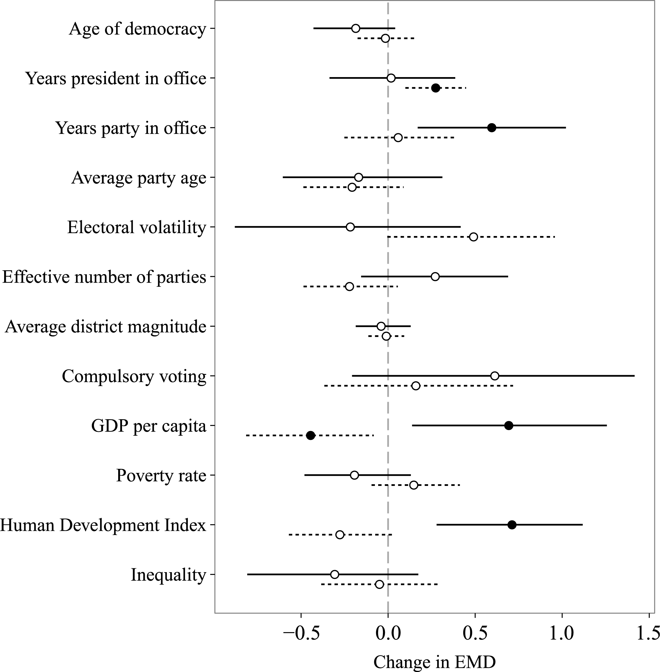
For each covariate, the top value in Figure 4 plots the predicted change in the multidimensional EMD as a result of shifting each independent variable across its interquartile range. For comparison, the bottom value plots the same predicted change, but using a unidimensional EMD based only on the left–right variable. Unlike previous studies, we find no relationship between congruence and political factors like the age of democracy or the institutionalization of the party system (proxied by average party age and electoral volatility). We also find no association between congruence and electoral institutions like compulsory voting or district magnitude. This is the case with both the unidimensional and multidimensional EMD. Whereas the number of years a president has been in office seems to be associated with only left–right congruence, the number of years the ruling party has been in office seems to significantly reduce overall congruence. In contrast to prior studies, we also find a statistically significant association between economic development and diminished mass–elite congruence, but only when we measure congruence across multiple dimensions.

Figure 4.

The correlates of mass–elite congruence in Latin America. Values represent the predicted effect on congruence of shifting each variable across its interquartile range, based on regression estimates reported in the online appendix. For each variable, the top value uses the multidimensional EMD measure and the bottom value measures the EMD with just left–right placement. Lines represent the bootstrapped 95% confidence intervals. Sources: See online appendix.

By measuring mass–elite congruence in Latin America with the EMD, we take advantage of its ability to summarize distances in high dimension. Our results stand in marked contrast to the claims of prior studies. Unlike previous scholars, we find no relationship between the institutionalization of a country’s party system and the level of congruence. Instead, we find that a ruling party’s tenure in office and economic development are correlated with congruence. Improving the way mass–elite congruence is measured yields very different substantive results that suggest that it is the countries in the region that are most developed where mass–elite congruence is lowest.

7 A New Measure for Comparing Distributions

How well do elected representatives reflect the preferences of the people who elected them? How and why does this level of mass–elite congruence vary over space and time? These are important questions not only for scholars of democratic representation but also for policymakers and activists seeking democratic reforms. They are fundamental if we wish to understand democratic representation and the contexts that help improve it. But to understand congruence and how it varies, we need to be able to measure it accurately.

The measures that currently prevail in political science— difference in means and CDF or PDF overlap—are woefully inadequate. They throw out sometimes enormous amounts of information in the data, they require arbitrary quantization choices that affect the measure, and they can only compute congruence along a single dimension. In contrast, the EMD resolves these problems. Because it uses signatures, the EMD does not require quantization or any other transformation of the data. It uses all of the information in the data and it works in high dimension. There are good theoretical reasons to prefer the EMD, and our simulations offer good empirical reasons as well.

The choice of measure is consequential. Measuring mass–elite congruence with the EMD affects our substantive claims. Whereas prior measures suggested a link between electoral rules and congruence, our reanalysis with the EMD uncovers no such relationship. We find no reason to think that PR systems yield more congruent legislatures than majoritarian ones. Whereas prior measures found positive correlations in Latin American democracies between congruence on the one hand and party system institutionalization and economic prosperity on the other, we find no such relationships. Instead, we find that socioeconomic factors like development are negatively associated with congruence.

The EMD gives a more accurate measure of congruence than those currently being used in political science. Moreover, it is simple to implement and offers scholars the ability to measure congruence in multiple dimensions. It should become the standard way we compute the distance between mass and elite preference distributions. Other research on representation could also employ the EMD: instead of comparing distributions of preferences, many studies of responsiveness compare mass opinion with policy outcomes (Bartels Reference Bartels2008; Gilens Reference Gilens2012; Canes-Wrone Reference Canes-Wrone2015). Here too the EMD can improve inferences.

More broadly, the EMD could be adopted whenever researchers want to compare distributions. Breunig and Jones (Reference Breunig and Jones2011) provide an extended discussion of how these kinds of comparisons can be used to test theories about budgetary processes. Scholars of U.S. politics have been debating whether American voters and political elites have become more polarized over time, and could employ the EMD to study long-term ideological shifts (e.g., Fiorina and Abrams Reference Fiorina and Abrams2008). Observers of Russian elections have compared the distribution of precincts’ reported turnout to uncover electoral fraud, and scholars of election forensics could use the EMD to measure similar electoral deviations from a baseline distribution (e.g., Myagkov, Ordeshook, and Shakin Reference Myagkov, Ordeshook and Shakin2005). Studies of between-group inequality could also use the EMD to quantify differences in income distributions across ethnic groups (Baldwin and Huber Reference Baldwin and Huber2010). For these and many other problems, the EMD is a useful and reliable way for political scientists to compare distributions.