


1 Introduction
The Honji instability, which is a three-dimensional (3-D) flow instability found in sinusoidally oscillatory flows around a stationary circular cylinder, was first reported by Honji (Reference Honji1981) and subsequently extensively investigated theoretically (e.g. Hall Reference Hall1984), experimentally (e.g. Sarpkaya Reference Sarpkaya2002) and numerically (e.g. An, Cheng & Zhao Reference An, Cheng and Zhao2011). This instability was classified as a regime B flow by Tatsuno & Bearman (Reference Tatsuno and Bearman1990), who systematically investigated the flow features induced by an oscillating circular cylinder through a visualisation technique and classified a total of six distinct flow regimes. These flow regimes cover a range of Keulegan–Carpenter numbers (
 $KC$
) and Stokes numbers (
 $\unicode[STIX]{x1D6FD}$
, or alternatively, the Reynolds number,
 $Re$
), which are defined as
 $$\begin{eqnarray}KC=U_{m}T/D,\quad Re=U_{m}D/\unicode[STIX]{x1D708},\quad \unicode[STIX]{x1D6FD}=Re/KC,\end{eqnarray}$$
where
 $U_{m}$
and
 $T$
are the amplitude and period of the oscillation velocity, respectively;
 $D$
is the cylinder diameter; and
 $\unicode[STIX]{x1D708}$
is the kinematic viscosity of the fluid.
The Honji instability arises at relatively low
 $KC$
and
 $\unicode[STIX]{x1D6FD}$
, and it gives rise to a series of mushroom-like flow structures that are evenly and periodically distributed along the cylinder surface in the spanwise direction, resulting from the detachment of the boundary layer from the surface of the cylinder and subsequent roll up of the boundary layer during each oscillation period. The Honji instability was found to be a centrifugal-type instability that is induced by the curvature of the boundary layer (Hall Reference Hall1984; Sarpkaya Reference Sarpkaya2002). The onset of the Honji instability is associated with the transition from a featureless two-dimensional (2-D) flow in regime
 $\text{A}^{\ast }$
to a 3-D flow in regime B, according to the nomenclature from Tatsuno & Bearman (Reference Tatsuno and Bearman1990).
Honji (Reference Honji1981) revealed that along any cross-sectional plane, the flow breaks the reflection symmetry with respect to the axis of flow oscillation due to the spanwise arrangement of mushroom vortices. The spanwise wavelength
 $\unicode[STIX]{x1D706}$
of the Honji vortex structure was found to be dependent on both
 $\unicode[STIX]{x1D6FD}$
and
 $KC$
. Hall (Reference Hall1984) conducted an asymptotic analysis under the assumption of
 $\unicode[STIX]{x1D6FD}\gg 1$
and small
 $KC$
and proposed a formula for the onset of the Honji instability in the
 $KC$
-
 $\unicode[STIX]{x1D6FD}$
space to estimate the threshold
 $KC$
and
 $\unicode[STIX]{x1D706}$
values (denoted as
 $KC_{h}$
and
 $\unicode[STIX]{x1D706}_{h}$
, respectively), which was named the ‘Hall line’ by Sarpkaya (Reference Sarpkaya2002). Sarpkaya (Reference Sarpkaya2002) observed that the Hall line is only relevant for persistent and fully developed coherent 3-D structures; however, below the Hall line, the flow is not absolutely stable against 3-D instabilities. Sarpkaya (Reference Sarpkaya2002) proposed an empirical formula to estimate the critical parameters,
 $KC_{s}$
and
 $\unicode[STIX]{x1D706}_{s}$
, for a 3-D instability, which is referred to as the ‘Sarpkaya line’ in the present study. Sarpkaya (Reference Sarpkaya2006) summarised the development process of 3-D flows as (I) no 3-D structures identifiable by flow visualisation for
 $KC<KC_{s}$
; (II) the quasi-coherent structure (QCS), which represents a 3-D flow structure formed under weaker instability than that required by Honji vortices for
 $KC_{s}<KC<KC_{h}$
; (III) the mushroom-shaped structures at
 $KC\approx KC_{h}$
; (IV) QCS again with further increase in
 $KC$
for
 $KC>KC_{h}$
; and (V) transition to chaotic motions and turbulence for large
 $KC$
values.
Elston, Blackburn & Sheridan (Reference Elston, Blackburn and Sheridan2006) conducted a Floquet stability analysis of the flow within the range of
 $KC\leqslant 10$
and
 $\unicode[STIX]{x1D6FD}\leqslant 100$
. The predicted marginal stability curve for the Honji instability is in good agreement with the regime boundary reported by Tatsuno & Bearman (Reference Tatsuno and Bearman1990) between regime
 $\text{A}^{\ast }$
and regime B. The critical
 $KC$
obtained from the Floquet stability analysis generally agrees with the ‘Hall line’ in the vicinity of the upper limit of the Stokes number (
 $\unicode[STIX]{x1D6FD}\approx 100$
). The predicted spanwise wavelength lies between the values given by Hall (Reference Hall1984) and Sarpkaya (Reference Sarpkaya2002). By examining the nonlinear properties of the bifurcation from regime
 $\text{A}^{\ast }$
to B, Elston et al. (Reference Elston, Blackburn and Sheridan2006) showed that the bifurcation is supercritical in the investigated range of
 $\unicode[STIX]{x1D6FD}$
.
An et al. (Reference An, Cheng and Zhao2011) numerically studied the generation and subsequent development of the Honji vortex over
 $100\leqslant \unicode[STIX]{x1D6FD}\leqslant 600$
and proposed that the spanwise wavelength of the Honji vortex is less dependent on
 $\unicode[STIX]{x1D6FD}$
and more sensitive to
 $KC$
(
 $\unicode[STIX]{x1D706}/D\sim 0.22KC^{7/4}$
) based on the numerical results and previous experimental observations (Honji Reference Honji1981; Tatsuno & Bearman Reference Tatsuno and Bearman1990; Bearman & Mackwood Reference Bearman and Mackwood1992; Sarpkaya Reference Sarpkaya2002). The interactions between adjacent vortices are characterised by the merging of adjacent vortices and the generation of new ones. Yang et al. (Reference Yang, Cheng, An, Bassom and Zhao2014) further outlined the three phases of the development of the Honji instability as (I) featureless two-dimensional flow, (II) evenly distributed and stable vortex pairs and (III) transient merging and axial shifting of vortex pairs. In addition, the effect of oblique incoming flow with regard to the axis of the cylinder was examined by Yang et al. (Reference Yang, Cheng, An, Bassom and Zhao2014), and it was found that the Honji instability is suppressed when the oblique angle is greater than a critical value.
Schematic diagram of a circular cylinder placed close to a plane boundary. The oscillatory flow is aligned with the
 $x$
-axis, which is parallel to the plane and perpendicular to the axis of the cylinder (defined as the
 $z$
-axis).
 $L_{x}$
,
 $L_{y}$
and
 $L_{z}$
represent the dimensions of the computational domain in the
 $x$
-,
 $y$
- and
 $z$
-directions, respectively.

For a cylinder near a plane boundary, as shown in figure 1, a third dimensionless parameter, namely, the gap ratio
 $e/D$
, becomes relevant, where
 $e$
denotes the distance between the plane boundary and the lower surface of the cylinder. For a partially embedded cylinder,
 $e/D$
has a negative value. Previous work on a cylinder near a plane boundary has mainly focused on the drag (
 $C_{D}$
) and inertia (
 $C_{M}$
) coefficients acting on the cylinder (Sarpkaya Reference Sarpkaya1976). It is understood that the force coefficients are dependent on
 $e/D$
. The in-line force per unit length in the form of Morison’s equation may be written as
 $$\begin{eqnarray}F_{x}=\frac{1}{2}\unicode[STIX]{x1D70C}DC_{D}|U|U+\frac{1}{4}\unicode[STIX]{x03C0}\unicode[STIX]{x1D70C}D^{2}C_{M}\frac{\text{d}U}{\text{d}t},\end{eqnarray}$$
where
 $F_{x}$
is the force in the direction of the oscillatory flow,
 $\unicode[STIX]{x1D70C}$
is the density of the fluid and
 $U(t)=U_{m}\sin (2\unicode[STIX]{x03C0}t/T)$
is the velocity of the ambient flow. In addition, the transverse lift coefficient (
 $C_{L}$
) is defined as
 $$\begin{eqnarray}F_{y}={\textstyle \frac{1}{2}}\unicode[STIX]{x1D70C}DC_{L}U_{m}^{2},\end{eqnarray}$$
where
 $F_{y}$
is the force perpendicular to the oscillatory flow.
 $C_{D}$
and
 $C_{M}$
are determined with the least squares method.
Xiong et al. (Reference Xiong, Cheng, Tong and An2018) recently investigated the oscillatory flow regimes and the onset of 2-D instabilities for a circular cylinder near a plane boundary at low-to-intermediate
 $KC$
numbers for
 $Re\leqslant 300$
and
 $e/D=0.25,0.5,1$
and
 $2$
. However, there has been no published study on the influence of a plane boundary on the development of the Honji instability. It is expected that the development of the Honji instability and the corresponding 3-D flow structures (including the spanwise wavelength) will be influenced by the existence of a plane wall and the oscillatory boundary layer developed on the plane. This expectation forms the motivation for this study. To limit the number of influencing factors, the present investigation is conducted at a fixed
 $KC$
of 2 over a range of
 $e/D$
(
 $-0.5\sim 2$
) and
 $\unicode[STIX]{x1D6FD}$
(up to 250). The remainder of this paper is organised as follows: the methodology and numerical model validation are introduced in § 2, the numerical results are discussed in § 3 and conclusions are drawn in § 4.
2 Methodology
The problem set-up and the computational domain are illustrated in figure 1, which is similar to that employed in Xiong et al. (Reference Xiong, Cheng, Tong and An2018). The free-stream oscillates along the
 $x$
-direction parallel to the plane boundary, perpendicular to the cylinder axis. As shown, the size of the computational domain is represented as
 $L_{x}\times L_{y}\times L_{z}$
.
The open source code Nektar++ (Cantwell et al.
Reference Cantwell, Moxey, Comerford, Bolis, Rocco, Mengaldo, De Grazia, Yakovlev, Lombard and Ekelschot2015), which is based on a Fourier spectral/
 $hp$
element method, is employed for the Floquet linear stability analysis and direct numerical simulation (DNS) in the present study. Although Nektar++ is well documented in the literature (e.g. Bolis Reference Bolis2013; Rocco Reference Rocco2014), it is briefly introduced below for the convenience of readers who are not necessarily familiar with the numerical approach.
The fluid motion is described by the incompressible Navier–Stokes (N–S) equations, expressed in a dimensionless form as
 $$\begin{eqnarray}\displaystyle & \displaystyle \frac{\unicode[STIX]{x2202}\boldsymbol{u}}{\unicode[STIX]{x2202}t}=-(\boldsymbol{u}\boldsymbol{\cdot }\unicode[STIX]{x1D735})\boldsymbol{u}-\unicode[STIX]{x1D735}p+Re^{-1}\unicode[STIX]{x1D6FB}^{2}\boldsymbol{u}, & \displaystyle\end{eqnarray}$$
 $$\begin{eqnarray}\displaystyle & \displaystyle \unicode[STIX]{x1D735}\boldsymbol{\cdot }\boldsymbol{u}=0, & \displaystyle\end{eqnarray}$$
where
 $\boldsymbol{u}$
is the velocity vector and
 $p$
is the pressure. The velocity components are referred to as
 $u$
,
 $v$
and
 $w$
in the
 $x$
-,
 $y$
- and
 $z$
-directions, respectively. The velocity components have been normalised by the free-stream velocity amplitude
 $U_{m}$
, and the axes are normalised by the cylinder diameter
 $D$
.
The Fourier spectral/
 $hp$
element method embedded in Nektar++ consists of a spectral/
 $hp$
element method to discretise the problem spatially in the
 $(x,y)$
-plane and a Fourier expansion in the
 $z$
-direction to reveal the full 3-D features of the flow (Bolis Reference Bolis2013). In the
 $(x,y)$
-plane, the total resolution is determined by the distribution of
 $h$
-type elements and the interpolate order
 $N_{p}$
of Lagrange polynomials for the
 $p$
-type refinement. The 3-D velocity vector and pressure are expressed in the following forms:
 $$\begin{eqnarray}\displaystyle & \displaystyle \boldsymbol{u}(x,y,z,t)=\mathop{\sum }_{m=0}^{N-1}\boldsymbol{u}_{m}(x,y,t)\text{e}^{\text{i}(2\unicode[STIX]{x03C0}mD/L_{z})z}, & \displaystyle\end{eqnarray}$$
 $$\begin{eqnarray}\displaystyle & \displaystyle p(x,y,z,t)=\mathop{\sum }_{m=0}^{N-1}\hat{p}_{m}(x,y,t)\text{e}^{\text{i}(2\unicode[STIX]{x03C0}mD/L_{z})z}, & \displaystyle\end{eqnarray}$$
where each component of Fourier mode
 $\boldsymbol{u}_{m}$
is a complex number (real and imaginary parts) at a specific Fourier mode index
 $m\,(=0,\ldots ,\!\,N-1)$
, spanwise wavenumber
 $k=2\unicode[STIX]{x03C0}mD/L_{z}$
or spanwise wavelength
 $\unicode[STIX]{x1D706}/D=2\unicode[STIX]{x03C0}/k=L_{z}/(mD)$
. Thus,
 $N$
is the total number of Fourier modes, and
 $2N$
represents the spanwise resolution. Hence, only a 2-D mesh is required for this quasi-3-D approach, and it degenerates to 2-D DNS for
 $N=1$
.
The Floquet linear stability analysis is also performed on the same mesh to investigate the 3-D instability. This method has been widely used to investigate hydrodynamic instabilities (Barkley & Henderson Reference Barkley and Henderson1996; Elston et al.
Reference Elston, Blackburn and Sheridan2006). For this reason, this analysis is only described briefly below. The linearised continuity and N–S equations for flow perturbation,
 $\boldsymbol{u}^{\prime }$
, can be written as
 $$\begin{eqnarray}\displaystyle & \displaystyle \frac{\unicode[STIX]{x2202}\boldsymbol{u}^{\prime }}{\unicode[STIX]{x2202}t}=-\boldsymbol{U}\boldsymbol{\cdot }\unicode[STIX]{x1D735}\boldsymbol{u}^{\prime }-\boldsymbol{u}^{\prime }\boldsymbol{\cdot }\unicode[STIX]{x1D735}\boldsymbol{U}-\unicode[STIX]{x1D735}p^{\prime }+Re^{-1}\unicode[STIX]{x1D6FB}^{2}\boldsymbol{u}^{\prime }, & \displaystyle\end{eqnarray}$$
 $$\begin{eqnarray}\displaystyle & \displaystyle \unicode[STIX]{x1D735}\boldsymbol{\cdot }\boldsymbol{u}^{\prime }=0. & \displaystyle\end{eqnarray}$$
Floquet stability analysis examines the evolution of infinitesimal perturbations according to these linearised equations based on a
 $T$
-periodic base flow
 $\boldsymbol{U}$
, which was obtained through the aforementioned 2-D DNS. In the present study, the duration of base simulations is extended to 200 flow periods when the base flow is fully developed with a relative difference of lift and inline force less than
 $0.1\,\%$
between two successive flow periods. The solution of the perturbation equations is simplified as
 $\tilde{\boldsymbol{u}}(x,y,z,t)\exp (\unicode[STIX]{x1D70E}T)$
, where
 $\tilde{\boldsymbol{u}}(x,y,z,t)$
holds
 $T$
-periodicity and
 $\unicode[STIX]{x1D70E}$
is the Floquet exponent. The Floquet multiplier
 $\unicode[STIX]{x1D707}=\exp (\unicode[STIX]{x1D70E}T)$
is used to identify the instability of the flow. Instability occurs when the Floquet multiplier leaves the unit circle, i.e.
 $|\unicode[STIX]{x1D707}|>1$
(perturbation increases exponentially), while stability is signalled when the multiplier is inside the unit circle, i.e.
 $|\unicode[STIX]{x1D707}|<1$
(perturbation decays exponentially).
A further simplification on the perturbation is made through a Fourier integral for both velocity and pressure (the expression for pressure is omitted for simplicity):
 $$\begin{eqnarray}\tilde{\boldsymbol{u}}(x,y,z,t)=\int _{-\infty }^{\infty }\tilde{\boldsymbol{u}}(x,y,k,t)\text{e}^{\text{i}kz}\,\text{d}k.\end{eqnarray}$$
Note that the spanwise wavenumber
 $k$
corresponds to the wavelength
 $\unicode[STIX]{x1D706}$
of the perturbation as
 $\unicode[STIX]{x1D706}/D=2\unicode[STIX]{x03C0}/k$
. Because modes with different
 $k$
do not couple, the Floquet multiplier for each
 $k$
can be obtained individually via a subspace iteration method. The iteration is performed on a Krylov subspace of 16 dimensions (referring to Rocco Reference Rocco2014), initialised from a random starting vector. Zero homogeneous velocity and high-order pressure boundary conditions are applied on all boundaries (Elston et al.
Reference Elston, Blackburn and Sheridan2006). The leading eigenvalue and eigenmode are obtained by applying the above operation on a range of
 $k$
.
The boundary conditions for a 2-D base flow or 3-D DNS are specified as follows. The free-stream velocity is specified at the top boundary as
 $U(t)=U_{m}\sin (2\unicode[STIX]{x03C0}t/T)$
. Zero Dirichlet velocity boundary conditions are applied on the cylinder surface and the plane boundary (unless otherwise specified). As in Elston et al. (Reference Elston, Blackburn and Sheridan2006), a high-order Neumann pressure boundary condition (Blackburn & Henderson Reference Blackburn and Henderson1999) is adopted on the 2-D domain boundaries, with one degree of freedom fixed at zero to avoid the singular pressure-Poisson problem (Bolis Reference Bolis2013). Periodic conditions are naturally imposed on the two lateral boundaries for the quasi-3-D approach. As for the choice of the inlet and outlet boundary conditions, different options are available. For example, Shen & Chan (Reference Shen and Chan2013) adopted the Dirichlet velocity boundary condition at the inlet and the Neumann velocity boundary condition at the outlet. Scandura, Armenio & Foti (Reference Scandura, Armenio and Foti2009) employed a periodic boundary condition in the streamwise direction. An, Cheng & Zhao (Reference An, Cheng and Zhao2010) adopted the Dirichlet velocity boundary condition with streamwise velocity component
 $U(y)\sin (2\unicode[STIX]{x03C0}t/T)$
and zero transverse velocity on both inlet and outlet boundaries, where
 $U(y)$
was specified in their equation (1). Xiong et al. (Reference Xiong, Cheng, Tong and An2018) demonstrated that the choice of inlet and outlet boundary conditions have little influence on the numerical results as long as the inlet and outlet boundaries are located sufficiently far away from the cylinder location. In the present study, the velocity boundary condition on the inlet and outlet is specified as
 $\boldsymbol{u}=(u_{s}(y,t),0,0)$
for DNS, where the streamwise velocity component
 $u_{s}(y,t)$
is obtained from the classical Stokes flow solution:
 $$\begin{eqnarray}u_{s}(y,t)=U(t)-\text{e}^{-\unicode[STIX]{x1D702}_{s}}U(t)\sin (2\unicode[STIX]{x03C0}t/KC-\unicode[STIX]{x1D702}_{s}),\quad \unicode[STIX]{x1D702}_{s}=\sqrt{\unicode[STIX]{x03C0}\unicode[STIX]{x1D6FD}}(y+D/2+e).\end{eqnarray}$$
Because the perturbed flow
 $\boldsymbol{U}+\boldsymbol{u}^{\prime }$
was recommended to satisfy the same boundary conditions as the base flow
 $\boldsymbol{U}$
(Barkley & Henderson Reference Barkley and Henderson1996), the zero homogeneous boundary condition is applied for Floquet stability analysis in the present study, which is similar to that employed in Elston et al. (Reference Elston, Blackburn and Sheridan2006).
The computational domain size is chosen based on an independent study by Scandura et al. (Reference Scandura, Armenio and Foti2009), where a domain size of up to
 $L_{x}\times L_{y}=46D\times 23D$
was used for a flow with
 $KC=10$
. A relatively conservative choice of
 $L_{x}\times L_{y}=60D\times (30D+e)$
is employed for the present case with
 $KC=2$
. The
 $h$
-type mesh is plotted with refinement on the surface of the cylinder and plane boundary. Consequently, 16
 $h$
-type boundary elements are specified on the circumference of the cylinder, and the radial density of the mesh decreases with increasing distance from the cylinder surface and plane boundary. This leads to the number of
 $h$
-type elements ranging from 1627 to 2841 for different
 $e/D$
values.
(a) A typical 2-D structured
 $h$
-type mesh at
 $e/D=0.5$
, with (b) a close-up view of the
 $hp$
-type mesh near the cylinder at the Lagrange interpolate order
 $N_{p}=8$
, where the nodal points of the spectral elements are determined from the zeros of the Gauss–Lobatto–Legendre polynomials (Karniadakis & Sherwin Reference Karniadakis and Sherwin2013).

A careful mesh sensitivity study was performed to investigate the convergence of interpolate order (
 $N_{p}$
), which is detailed in § A.1. According to the results,
 $N_{p}=8$
is employed for all simulations. For this mesh, a total of 129 azimuthal points are evenly distributed on the circumference of the cylinder, and the distance between the first layer of grid points away from the no-slip boundaries (cylinder surface and plane boundary) is approximately
 $0.1\unicode[STIX]{x1D6FF}$
, where
 $\unicode[STIX]{x1D6FF}$
is the boundary layer thickness and is estimated by
 $\unicode[STIX]{x1D6FF}/D=0.75\unicode[STIX]{x03C0}(\unicode[STIX]{x03C0}\unicode[STIX]{x1D6FD})^{-1/2}$
(Carstensen, Sumer & Fredsøe Reference Carstensen, Sumer and Fredsøe2010). An example of the 2-D mesh chosen for
 $e/D=0.5$
is presented in figure 2, including the
 $h$
-type mesh on the left and the
 $hp$
-refinement near the cylinder on the right. The spanwise length
 $L_{z}=5.6D$
and spanwise resolution
 $2N=64$
are also determined from the mesh sensitivity study presented in appendix A.
Vortex iso-surfaces around an isolated cylinder for
 $(KC,\unicode[STIX]{x1D6FD})=(2,200)$
at
 $t/T=100$
.

3 Results and discussion
3.1 Wall-free case
The Honji instability developed around an isolated circular cylinder at
 $KC=2$
and
 $\unicode[STIX]{x1D6FD}=200$
is visualised through the iso-surface of vorticity components in figure 3 to further validate the model and to facilitate the following discussion on the influence of the plane boundary proximity. The streamwise vorticity
 $\unicode[STIX]{x1D714}_{x}$
reveals the presence of 8 pairs of rib-like vortices that are evenly distributed on the surface of the cylinder, where the cylinder has a spanwise length of
 $5.6D$
. This observation is consistent with the distributions of
 $\unicode[STIX]{x1D714}_{y}$
and
 $\unicode[STIX]{x1D714}_{z}$
, as well as with those reported by An et al. (Reference An, Cheng and Zhao2011).
Comparison of the predicted critical
 $KC$
number (a) and wavelength (b) for the Honji instability of an isolated cylinder with results published in the literature. Hall (Reference Hall1984) line:
 $KC_{h}=5.788\unicode[STIX]{x1D6FD}^{-1/4}(1+0.205\unicode[STIX]{x1D6FD}^{-1/4})$
,
 $\unicode[STIX]{x1D706}_{h}/D=6.95\unicode[STIX]{x1D6FD}^{-1/2}$
; Sarpkaya (Reference Sarpkaya2002) line:
 $KC_{s}=12.5\unicode[STIX]{x1D6FD}^{-2/5}$
,
 $\unicode[STIX]{x1D706}_{s}/D=22\unicode[STIX]{x1D6FD}^{-3/5}$
.

Figure 4 presents a comparison of the present critical
 $KC$
number and wavelength for the onset of the Honji instability and those reported in the literature for an isolated cylinder. Through Floquet stability analysis, the predicted marginal curves on
 $KC_{cr}$
and
 $\unicode[STIX]{x1D706}_{cr}/D$
and the most unstable mode of the 3-D instability at
 $KC=2.58$
and
 $\unicode[STIX]{x1D6FD}=80$
, as shown in figure 5, agree well with those reported by Elston et al. (Reference Elston, Blackburn and Sheridan2006). The present results also largely agree with the experimental data of Tatsuno & Bearman (Reference Tatsuno and Bearman1990). This finding demonstrates that the numerical model is capable of accurately predicting the Honji instability. Specifically, the marginal stability for the wall-free case at
 $KC=2$
is observed at
 $\unicode[STIX]{x1D6FD}_{cr_{\infty }}=140$
and
 $\unicode[STIX]{x1D706}_{cr_{\infty }}/D=0.72$
.
Comparison of instantaneous iso-surfaces of
 $x$
-vorticity of the critical 3-D instability for an isolated cylinder at
 $(KC,\unicode[STIX]{x1D6FD},k)=(2.58,80,5.88)$
between (a) Elston et al. (Reference Elston, Blackburn and Sheridan2006) and (b) the present study. The arrow indicates the direction of flow oscillation.

Note that a relatively clear difference exists between the experimental data (Tatsuno & Bearman Reference Tatsuno and Bearman1990) and the results of Hall (Reference Hall1984). This difference is possibly because the Hall line was obtained assuming that
 $\unicode[STIX]{x1D6FD}\gg 1$
, which is not the case for the parameter space shown in figure 4. The difference between the experimental data (Tatsuno & Bearman Reference Tatsuno and Bearman1990) and the results of Sarpkaya (Reference Sarpkaya2002) is likely because the weak 3-D QCS was considered in the Sarpkaya line.
3.2 Marginal curve for Honji instability
The influence of the plane boundary on the initiation of the Honji instability is first investigated by quantifying the variation in the marginal stability with
 $e/D$
through Floquet stability analysis at
 $KC=2$
and eleven gap ratios, i.e.
 $e/D=-0.5,-0.25,-0.125,0.03125,0.0625,0.125,0.25,0.375,0.5,1$
and
 $2$
. The variations in the marginal stability (
 $\unicode[STIX]{x1D6FD}_{cr}$
) and critical spanwise wavelength (
 $\unicode[STIX]{x1D706}_{cr}/D$
) with
 $e/D$
are summarised in figure 6. As expected, both
 $\unicode[STIX]{x1D6FD}_{cr}$
and
 $\unicode[STIX]{x1D706}_{cr}/D$
asymptote towards their counterparts for an isolated cylinder at large gap ratios (e.g.
 $e/D=2$
) due to the weak influence of the plane boundary. It is also clear that the variations in
 $\unicode[STIX]{x1D6FD}_{cr}$
and
 $\unicode[STIX]{x1D706}_{cr}/D$
with
 $e/D$
have opposite trends.
Critical Stokes number
 $\unicode[STIX]{x1D6FD}_{cr}$
(a) and the corresponding spanwise wavelength
 $\unicode[STIX]{x1D706}_{cr}/D$
(b) as a function of gap ratios for the onset of the Honji instability at
 $KC=2$
(solid lines). The thick dashed line represents the extrapolation based on the data points at
 $e/D=0.125$
. The horizontal dotted line denotes the value for an isolated cylinder, and vertical dotted lines running through
 $e/D=0$
and
 $0.125$
are provided for reference.

As the cylinder is moved towards the wall, the marginal stability exhibits a few distinctive features. First, as
 $e/D$
is reduced from
 $2$
to
 $0.375$
,
 $\unicode[STIX]{x1D6FD}_{cr}$
decreases from
 $134$
at
 $e/D=2$
to
 $100$
at
 $e/D=0.375$
, which suggests an enhancement in the marginal Honji instability with the reduction of
 $e/D$
in that range. With a further decrease of
 $e/D$
from
 $0.375$
to
 $0.125$
,
 $\unicode[STIX]{x1D6FD}_{cr}$
increases and reaches a peak value of approximately
 $205$
, which is considerably higher than
 $140$
for an isolated cylinder. This result suggests weakening of the marginal Honji instability with the reduction of
 $e/D$
for
 $0.125<e/D<0.375$
. The enhancement and weakening of the marginal Honji instability are again observed for
 $0.03125\leqslant e/D<0.125$
and
 $e/D<0$
, respectively. Note that the
 $\unicode[STIX]{x1D6FD}_{cr}\approx 205$
at
 $e/D=0.125$
is actually obtained using DNS rather than through Floquet stability analysis. This is because the breaking of two-dimensional symmetry (spatio-temporal) occurs at a smaller
 $\unicode[STIX]{x1D6FD}$
than that for the three-dimensional instability, which makes the Floquet stability analysis invalid at
 $e/D=0.125$
. The breaking of 2-D symmetry at
 $e/D=0.125$
is illustrated in figure 7 for
 $\unicode[STIX]{x1D6FD}=200$
and
 $210$
, while the flow with
 $\unicode[STIX]{x1D6FD}=160$
possesses spatio-temporal symmetry. It will be shown later that the
 $\unicode[STIX]{x1D6FD}_{cr}\approx 205$
at
 $e/D=0.125$
is due to a different three-dimensional instability from the Honji instability.
Comparison of instantaneous vorticity contours based on 2-D DNS at
 $e/D=0.125$
. (a)
 $\unicode[STIX]{x1D6FD}=160$
, (b)
 $\unicode[STIX]{x1D6FD}=200$
and (c)
 $\unicode[STIX]{x1D6FD}=210$
. Two instants are given at
 $t/T=150$
(top) and
 $150.5$
(bottom).

Comparison of profiles of peak velocity components against
 $y/D$
for different gap ratios at
 $\unicode[STIX]{x1D6FD}=150$
from 2-D base flow
 $\boldsymbol{U}$
: (a) at the gap side and (b) at the top free-stream side. They are sampled along the line at
 $x=0$
during one cycle of oscillation (thus, the peak velocities do not necessarily occur at the same time instant).

The flow mechanisms responsible for the variation trend of the marginal stability curve with
 $e/D$
in figure 6 are explained below.
(i) The enhancement of the marginal Honji instability for
 $e/D\geqslant 0.375$
(up to 2) is primarily attributed to the local blockage effect, where the geometry setting of the plane boundary and the cylinder introduces an asymmetric distribution of fluid flow about the
 $x$
-axis and enhances the flow through the gap. The increased peak flow velocity (in both the horizontal and vertical components) on the gap side is shown in figure 8, which leads to the occurrence of the marginal Honji vortices on the gap side of the cylinder surface first. This is evidenced by the 3-D flow structures shown in figure 9(a,b) for the critical 3-D instability, where the Honji vortices appear on both the top and bottom sides of the cylinder surface for an isolated cylinder but are only present on the gap side for
 $e/D=1$
.
Comparison of instantaneous
 $x$
-vorticity iso-surfaces of the critical 3-D instability for (a)
 $e/D=\infty$
, (b)
 $1$
, (c)
 $0.25$
and (d)
 $-0.5$
. Three spanwise repetitions are illustrated at the instant of
 $t_{0}=0$
.

Variation of pressure drop between sampling points A and B as a function of gap ratio at
 $\unicode[STIX]{x1D6FD}=140$
.

(ii) The weakening of the marginal Honji instability for
 $0.125\leqslant e/D<0.375$
is associated with the transition of the onset of the marginal instability from the gap side to the top side of the cylinder surface (figure 9
c), which is referred to as side swapping hereafter. This side swapping is mainly caused by two flow mechanisms. One is the reduction in the curvature of the flow trajectory through the gap, as evidenced in figure 8(a), where a substantial reduction in
 $|V_{max}|$
is observed as
 $e/D$
is reduced from
 $0.375$
to
 $0.125$
. It is believed that the magnitude of
 $|V_{max}|$
correlates positively with the curvature of the flow trajectory. Since the Honji instability is a centrifugal-type instability, a reduction in the curvature of the flow trajectory is thought to stabilise the flow. The other reason is associated with the increase in the favourable pressure gradient through the gap, where a favourable pressure gradient in the flow direction is known to increase the flow stability by hydrodynamic stability theories (Reed, Saric & Arnal Reference Reed, Saric and Arnal1996). To support this, a period-averaged pressure gradient over the gap at
 $\unicode[STIX]{x1D6FD}=140$
is quantified in figure 10. A substantial increase in the favourable pressure gradient (from A to B) over the gap section of the plane boundary is observed as
 $e/D$
is reduced from
 $0.375$
to
 $0.125$
. The combination of the two mechanisms suppresses the occurrence of the Honji instability on the gap side of the cylinder surface, leading to the side swapping and the increase in
 $\unicode[STIX]{x1D6FD}_{cr}$
with decreasing
 $e/D$
. The side swapping phenomenon is illustrated through the instantaneous kinetic energy of the leading eigenmode in figure 11, where the location of the marginal instability is indicated by the location of the maximum kinetic energy of the leading eigenmode. It is observed that the marginal instability appears on the gap side at
 $e/D\geqslant 0.375$
and on the top side at
 $e/D\leqslant 0.25$
(except the case at
 $e/D\approx 0.125$
).
(iii) The enhancement in the marginal flow instability at
 $0.03125\leqslant e/D<0.125$
is attributed to the increase in the peak flow (horizontal) velocity on the top side of the cylinder as
 $e/D$
is reduced, as evidenced in figure 8(b), while the weakening of the marginal Honji instability for
 $e/D<0$
is caused by the decrease in the peak horizontal velocity on the top side as the embedment depth is increased.
Contours of
 $\unicode[STIX]{x1D714}_{z}$
of the base flow and instantaneous kinetic energy of the leading eigenmode at (a)
 $(e/D,\unicode[STIX]{x1D6FD},\unicode[STIX]{x1D706}/D)=(\infty ,140,0.739)$
, (b)
 $(1,130,0.785)$
, (c)
 $(0.375,105,1.047)$
, (d)
 $(0.25,150,0.739)$
, (e)
 $(0.03125,80,0.967)$
and (f)
 $(-0.5,190,0.628)$
. No colour legend is given for kinetic energy because the eigenmodes are normalised by setting the value of integration over the domain equal to 1, but a dark colour still corresponds to higher energy and light colour corresponds to lower energy.
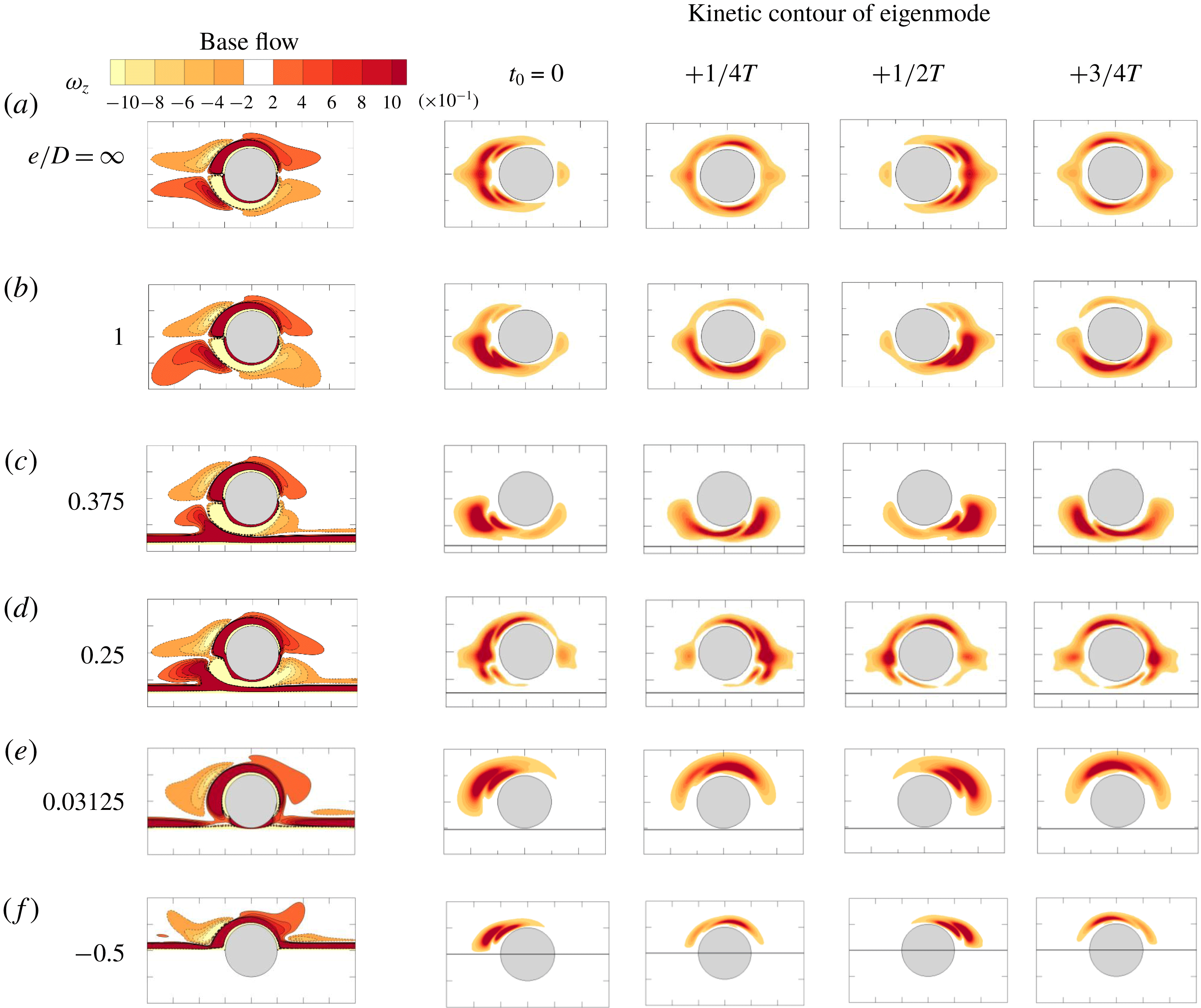
In figure 11, the effect of
 $e/D$
on the Honji instability is further examined by contours of
 $z$
-vorticity of the base flow and kinetic energy of the leading eigenmode, which is defined by
 $$\begin{eqnarray}E_{k}(t)=\frac{1}{2}\int _{\unicode[STIX]{x1D6FA}}\Vert \hat{\boldsymbol{u}}_{k}\Vert ^{2}\,\text{d}\unicode[STIX]{x1D6FA}.\end{eqnarray}$$
For the isolated cylinder, the 3-D instability is symmetric and appears in the near-cylinder region (figure 11
a). At
 $e/D=1$
and
 $0.375$
, the kinetic energy of the leading eigenmodes is mainly concentrated on the gap side (figure 11
b and c), suggesting that the instability is initiated from the gap side, in agreement with the blockage effect as identified above. In contrast, the large kinetic energy of the leading eigenmode for
 $e/D=0.25$
and
 $0.03125$
is mainly distributed over the top side of the cylinder and in turn suggests the location for the initiation of the instability. Note that the leading eigenmodes on the top side of the cylinder at
 $e/D=0.25$
(figure 11
d) are similar to half of those of an isolated cylinder (figure 11
a), whereas the kinetic energy at the gap side almost completely disappears. The leading eigenmodes at
 $e/D\leqslant 0.03125$
only appear on the top side (figure 11
e and f), and the weak vorticity contour on the bottom side is consistent with the low flow velocity as shown in figure 8.
Regime map in
 $(e/D,\unicode[STIX]{x1D6FD})$
-plane at
 $KC=2$
based on the formation of Honji vortices on the top and gap sides of the cylinder. The status on the top or gap side of the cylinder is detected by probe lines at
 $(x,y)=(0,\pm 0.51D)$
, and each is represented by a half-marker in the legend. The solid line was reproduced from the marginal curve in figure 6 for comparison, while the dashed marginal line is estimated from the 3-D DNS results. The arrows and sequence numbers denote that the parameters are discussed specifically in §§ 3.3.1–3.3.4, respectively.

Recalling the critical wavelength
 $\unicode[STIX]{x1D706}_{cr}/D$
of the marginal Honji instability in figure 6(b), it is believed that the physical mechanisms responsible for the trend are the same as those identified above. For example, the increasing trend of
 $\unicode[STIX]{x1D706}_{cr}/D$
for
 $0.375\leqslant e/D\leqslant 2.0$
is induced by the velocity increase of the gap flow. The local velocity increase leads to an increase in the value of effective
 $KC(=U_{m}T/D)$
. As reported by An et al. (Reference An, Cheng and Zhao2011),
 $\unicode[STIX]{x1D706}/D$
is directly dependent on
 $KC$
as
 $\unicode[STIX]{x1D706}/D\sim 0.2(KC)^{7/4}$
. A quantitative estimate of the increase in
 $\unicode[STIX]{x1D706}_{cr}/D$
at
 $e/D=0.375$
(figure 6
b) is thus made based on the peak gap velocity shown in figure 8 and the formula proposed by An et al. (Reference An, Cheng and Zhao2011). The peak velocity ratio (which equals the
 $KC$
ratio as shown in (1.1a–c
)) of
 $e/D=0.375$
to
 $e/D=2.0$
is approximately 1.28, and this leads to an increase ratio of
 $\unicode[STIX]{x1D706}_{cr}/D$
at 1.55. The actual increase ratio is approximately 1.42 from the stability analysis in figure 6(b). Although such an estimate is only indicative, it illustrates one of the causes behind the change in
 $\unicode[STIX]{x1D706}_{cr}/D$
with
 $e/D$
. In general, the change in
 $\unicode[STIX]{x1D706}_{cr}/D$
with
 $e/D$
corresponds well to the variation trend of peak velocities either through the gap or on the top side of the cylinder.
3.3 Three-dimensional flow structures and regime classification
A set of DNSs is also conducted at
 $KC=2$
and
 $\unicode[STIX]{x1D6FD}=75\sim 250$
for all gap ratios listed earlier to further examine the flow structures and the physical mechanisms that are responsible for the observed effects of
 $e/D$
on the Honji instability.
Four distinctive flow regimes on the (
 $e/D$
,
 $\unicode[STIX]{x1D6FD}$
)-plane are observed and classified (I, II, III and IV) in figure 12. These regimes are as follows:
(I) featureless two-dimensional flow, where there is no Honji vortex structure;
(II) stable Honji vortex, where the classical Honji instability appears with a distinctive and stable spanwise length;
(III) unstable Honji vortex, where neighbouring Honji vortices merge and generate new ones; and
(IV) chaotic flow, which is characterised by significant turbulent flows.
Due to the influence of the plane boundary, the flow regimes on the gap and top sides of the cylinder are generally not the same, depending on
 $e/D$
and
 $\unicode[STIX]{x1D6FD}$
. To distinguish this interesting flow feature, each marker used to represent a flow regime in figure 12 consists of a top part and a bottom part, indicating the flow regime on the top and bottom parts of the cylinder. Note that the boundary that separates regimes (I) and (II) agrees very well with the marginal stability curve derived from the Floquet stability analysis. Compared to that of an isolated cylinder, the Honji instability is suppressed at approximately
 $e/D=0.125$
, but it is enhanced at intermediate gap ratios (
 $e/D\geqslant 0.375$
), where it occurs at smaller
 $\unicode[STIX]{x1D6FD}$
values. For
 $e/D\leqslant 0.03125$
, a stable Honji vortex structure only occurs on the top side of the cylinder. In addition, regime (III) appears only for intermediate gap ratios with
 $\unicode[STIX]{x1D6FD}$
between 200 and 250. Chaotic 3-D structures occur at
 $e/D=0.125$
and
 $0.25$
at
 $\unicode[STIX]{x1D6FD}=250$
.
The influence of the plane boundary and
 $\unicode[STIX]{x1D6FD}$
on Honji flow structures is further investigated in the following four sections at fixed
 $\unicode[STIX]{x1D6FD}=150$
(§ 3.3.1) and
 $250$
(§ 3.3.2), as well as at constant
 $e/D=0.125$
(§ 3.3.3) and
 $0.375$
(§ 3.3.4), as indicated by the arrows in figure 12.
Comparison of iso-surfaces of
 $Q=0.25$
(yellow) and
 $x$
-vorticity
 $\unicode[STIX]{x1D714}_{x}=\pm 0.5$
(translucent in red and blue) at
 $\unicode[STIX]{x1D6FD}=150$
at phase
 $t_{0}=0$
.

3.3.1
 $\unicode[STIX]{x1D6FD}=150$

The influence of the plane boundary on the Honji vortex structure is first examined at
 $\unicode[STIX]{x1D6FD}=150$
. Figure 13 illustrates typical 3-D flow visualisations at eight representative gap ratios. The vortical flow structure is visualised by employing the instantaneous iso-surfaces of
 $x$
-vorticity and
 $Q$
(Hussain Reference Hussain1986), which is a criterion for distinguishing an eddy from the plane shear layer. The eddy is defined in the region by the positive second invariant,
 $Q$
of
 $\unicode[STIX]{x1D735}\boldsymbol{u}$
, with an additional condition that the pressure is lower than the ambient value. The second invariant
 $Q$
is defined as
 $$\begin{eqnarray}Q={\textstyle \frac{1}{2}}(\Vert \unicode[STIX]{x1D6FA}\Vert ^{2}+\Vert S\Vert ^{2}),\end{eqnarray}$$
where
 $S$
and
 $\unicode[STIX]{x1D6FA}$
are the symmetric and antisymmetric components of
 $\unicode[STIX]{x1D735}\boldsymbol{u}$
, respectively.
Figure 13 visually shows that stable Honji vortex pairs appear on the top side of the cylinder surface for
 $-0.5<e/D<0.125$
and on both the top and gap sides of the cylinder for
 $e/D\geqslant 0.25$
, except for
 $e/D=-0.5$
and
 $0.125$
, where no Honji vortex pairs are captured. It is observed that the Honji vortex structure at
 $e/D=2$
is similar to that of an isolated cylinder (figure 13
a), while at
 $e/D=-0.25$
(figure 13
g), it is similar to half of the structure on an isolated cylinder, suggesting that the flow around a partially embedded cylinder shares a similar mechanism for transitioning to three dimensions with an isolated cylinder.
Apart from the obvious Honji vortex structures, spanwise vortex tubes are also observed at
 $e/D=0.25\sim 0.5$
in figure 13(b–d). The mechanisms for the formation of spanwise vortex tubes are likely due to the roll up of the shear layers of the cylinder and over the plane boundary. The vortex tubes are largely two-dimensional and attached to the cylinder surface or the plane boundary with weak three-dimensionality at
 $\unicode[STIX]{x1D6FD}=150$
. It will be shown later that these spanwise vortex tubes will have significant influences on the formation of Honji vortex structures at small gap ratios (e.g.
 $e/D<0.5$
).
Comparison of profiles of peak velocity components against
 $y/D$
for different gap ratios at
 $\unicode[STIX]{x1D6FD}=150$
: (a) at the gap side and (b) at the top side. Velocity components are sampled along the line at
 $x=0$
during one cycle of oscillation.

The flow characteristics at
 $\unicode[STIX]{x1D6FD}=150$
are further quantified in figure 14 by the peak velocity components in all three directions, denoted by
 $u_{max}$
,
 $v_{max}$
and
 $w_{max}$
, respectively, along
 $x=0$
, which is a 3-D version of figure 8. There is no obvious difference between the 2-D and 3-D velocity profiles of
 $|u_{max}|$
, but the 3-D results of
 $|v_{max}|$
are generally larger than their 2-D counterparts due to the upward rolling flow structures, including the Honji vortex. At the gap side (
 $y<-0.5$
),
 $u_{max}$
shows a monotonic increase with the decrease of
 $e/D$
until
 $e/D=0.125$
and then a sudden decrease to
 $e/D=0.03125$
. The
 $|w_{max}|$
and
 $|v_{max}|$
all increase with decreasing
 $e/D$
for
 $e/D>0.375$
and reach the maximum values at
 $e/D=0.375$
. A further decrease of
 $e/D$
for
 $e/D<0.375$
leads to sharp decreases in
 $|w_{max}|$
and
 $|v_{max}|$
. The spanwise velocity component
 $|w_{max}|$
vanishes at
 $e/D\leqslant 0.125$
, marking the disappearance of three-dimensional flow. Similarly, the Honji instability is of a centrifugal type in nature, and a large curvature of the flow trajectory (which positively correlates with the magnitude of
 $|v_{max}|$
) corresponds to a strong Honji vortex structure. Thus,
 $u_{max}$
,
 $v_{max}$
and
 $w_{max}$
all reach the maximum at
 $e/D=0.03125$
on the top side of the cylinder.
(a,b) Comparison of characteristic normalised wavenumber
 $m$
by
 $w$
-velocity obtained along two probe lines, where the fast Fourier transform (FFT) results are averaged after
 $t/T=20$
; (c) the spectrum square root of mean modal kinetic energy; (d) the phase variation of square root of overall 3-D (
 $k\not =0$
) kinetic energy during one cycle obtained by phase averaging; (e) comparison of mean overall kinetic energy; and (f) effective wavelength. All the results are at
 $\unicode[STIX]{x1D6FD}=150$
.

The influence of the wall proximity on Honji vortex structures can also be quantified by examining the spectra of the
 $w$
-velocity by performing a fast Fourier transform (FFT) on velocity signals sampled at the top and bottom probe lines at
 $x=0$
and
 $y=\pm 0.51D$
in figure 15(a,b). For simplicity, the Fourier mode index
 $m=kL_{z}/(2\unicode[STIX]{x03C0}D)$
is referred to as normalised wavenumber hereafter to facilitate the discussion. Here, the spectrum represents the strength of the 3-D flow structures as a function of
 $m$
. A spectrum range of
 $4\leqslant m\leqslant 20$
is selected, mainly because the spectrum amplitudes outside this range are trivial (except at
 $m=0$
, which corresponds to the 2-D flow component if applicable). The influence of the wall proximity on Honji structures is clearly observed. As
 $e/D$
is reduced from
 $2.0$
to
 $0.375$
, the amplitudes of
 $|w_{m}|$
spectra increase noticeably on the gap side (correspondingly, the Honji structure is enhanced) and decrease slightly on the top side (the Honji structure is weakened). This is also supported by the generally larger peak amplitudes of
 $|w_{m}|$
spectra on the gap side than their counterparts on the top side. Specifically, figure 15(a) shows that the leading normalised wavenumber
 $m$
(i.e. the dominant spectrum peak) on the top side decreases from
 $m=8$
at
 $e/D=2$
to
 $m=7$
at
 $e/D=0.5$
and
 $0.375$
, while the leading
 $m$
on the gap side decreases from
 $m=8$
at
 $e/D=2$
to
 $m=7$
at
 $e/D=0.5$
and
 $m=6$
at
 $e/D=0.375$
. As
 $e/D$
is further reduced from
 $e/D=0.375$
to
 $0.125$
, the Honji instability is significantly weakened on both sides of the cylinder and disappears completely at
 $e/D=0.125$
, where the 3-D components all vanish and the flow becomes two-dimensional. This is consistent with the prediction by the Floquet stability analysis (figures 6 and 11
d). When
 $e/D$
is further reduced to
 $0.03125$
and
 $e/D<0$
, the Honji structure returns to the top side of the cylinder with
 $m=7$
at
 $e/D=0.03125$
and
 $m=8$
at
 $e/D=-0.25$
. The sharp peak at
 $e/D=0.03125$
on the top side of the cylinder suggests a well-defined Honji vortex structure.
The spanwise wavenumber is also investigated by examining the spectrum of the modal kinetic energy (
 $E_{m}$
), which represents the kinetic energy of Fourier mode
 $\hat{\boldsymbol{u}}_{m}$
, as defined similarly to that of the eigenmode in (3.1). Figure 15(c) and (d) show the spectrum of the total kinetic energy
 $E_{m}$
and phase variation of the total 3-D kinetic energy
 $E_{\text{3-D}}(t_{0}/T)=\sum _{m=1}^{N-1}\overline{E_{m}}(t_{0}/T)$
, where the phase
 $t_{0}/T$
is defined as
 $t_{0}/T=(t-nT)/T$
and
 $n$
is number of cycles for free-stream oscillation, and the total kinetic energy is the summation of
 $E_{m}$
from
 $m=1$
to
 $N-1$
. The value of
 $E_{3-D}(t_{0}/T)$
is phase averaged from
 $t/T=20$
and for at least 80 cycles. The modal kinetic energy
 $\sqrt{\overline{E_{m}}}$
in figure 15(c) represents the overall feature of the velocity field, as illustrated in figure 15(a) and (b). The 3-D energy is the highest at
 $e/D=0.03125$
, where the Honji instability reappears on the top side of the cylinder, and the second, third and fourth highest cases are at
 $e/D=0.375$
,
 $0.5$
and
 $2.0$
, respectively. Consistent with (a), the 3-D energy at
 $e/D=0.25$
is almost identical to that at
 $e/D=2.0$
, and the 3-D components all vanish at
 $e/D=0.125$
. The phase variation of the 3-D energy is also affected by the proximity of the wall. It peaks at a phase around
 $t_{0}/T=0$
(or
 $0.5$
) when the flow accelerates (or decelerates) for cases at
 $e/D=0.5$
and
 $0.375$
; however, it peaks at
 $t_{0}/T=0.25$
(or
 $0.75$
) when the free-stream velocity amplitude is the largest for cases at
 $e/D=0.03125$
and
 $-0.25$
.
The square root of the mean 3-D kinetic energy of the flow (
 $\sqrt{\overline{E}_{\text{3-D}}}$
) is quantified by removing the 2-D component (
 $m=0$
), which reflects the effective strength of the Honji instability. Figure 15(e) presents the variation in
 $\sqrt{\overline{E}_{\text{3-D}}}$
with
 $e/D$
, which has an opposite trend to that of
 $\unicode[STIX]{x1D6FD}_{cr}$
shown in figure 6(a). This result is expected because the enhancement of the Honji instability corresponds to an increase in the overall 3-D kinetic energy, and vice versa. The effective wavelength is shown in figure 15(f), which is obtained by the weighted average of the modal kinetic energy as
 $$\begin{eqnarray}\unicode[STIX]{x1D706}_{e}=L_{z}/m_{e},\quad m_{e}=\frac{\sum mE_{m}}{\sum E_{m}}.\end{eqnarray}$$
As shown in figure 15(f), the variation of effective wavelength
 $\unicode[STIX]{x1D706}_{e}/D$
with
 $e/D$
follows the same trend as that of
 $\unicode[STIX]{x1D706}_{cr}/D$
in figure 6(b).
Temporal and spatial evolution of the
 $w$
-velocity component sampled at
 $t_{0}/T=0.25$
along lines of
 $(x,y)=(0,0.51D)$
(a–f) and
 $(0,-0.51D)$
(g–l) for the case with
 $\unicode[STIX]{x1D6FD}=250$
at different gap ratios.

Iso-surfaces of
 $Q$
-criterion,
 $Q=0.25$
, at
 $\unicode[STIX]{x1D6FD}=250$
at
 $t_{0}=0$
for different gap ratios.

3.3.2
$\unicode[STIX]{x1D6FD}=250$

The flow structures at
 $\unicode[STIX]{x1D6FD}=250$
are in general similar to those at
 $\unicode[STIX]{x1D6FD}=150$
, except around
 $0<e/D<0.5$
, where the influence of the plane boundary leads to complex 3-D structures, including unstable Honji vortices and chaotic separated vortices at
 $\unicode[STIX]{x1D6FD}=250$
. Figure 16 illustrates the development of three-dimensionality at
 $\unicode[STIX]{x1D6FD}=250$
by the spatio-temporal contours of
 $w$
-velocity for selected
 $e/D$
, which are sampled along two probe lines located at
 $x=0$
and
 $y=\pm 0.51D$
in the spanwise direction and at a phase
 $t_{0}/T=0.25$
of each oscillation cycle. Each pair of dark and light colour stripes represents a pair of Honji vortices. It is observed that Honji vortex structures are temporally stable at
 $e/D=1$
, similar to that of the isolated cylinder. The Honji vortex structures are temporally unstable at the top sampling line at
 $e/D=0.375$
, featuring the coalescence of neighbouring vortices and the emergence of new vortices, which is similar to those shown in figure 14 of An et al. (Reference An, Cheng and Zhao2011). Apparent high-frequency variations in contours on the gap side at
 $e/D=0.125$
and
 $0.25$
indicate strong instabilities. No regular Honji structures are observed on the top part of the cylinder at
 $e/D=0.125$
, although the flow is clearly three-dimensional and is considered to be chaotic flow here. At
 $e/D=0.03125$
, the stripes on the top side indicate stable and regular Honji vortices. The strength and the number of strips at the top and gap sides of the cylinder are not equal, which will be detailed later.
The 3-D flow structures are shown by translucent iso-surfaces of
 $Q=0.25$
in figure 17. For all selected cases, the Honji vortex structures on the top side of the cylinder are similar, except for the case at
 $e/D=0.125$
, where coherent structures almost completely disappear and are replaced by small 3-D flow structures. At
 $e/D=1$
, the Honji vortex on the gap side is almost identical to that on the top side, but the difference becomes more obvious with decreasing
 $e/D$
. The attached vortex tubes observed at
 $\unicode[STIX]{x1D6FD}=250$
are not clearly visible and are believed to evolve into highly twisted 3-D flow structures, as shown in figure 17(b–d). The gap vortex shedding is believed to be responsible for these irregular 3-D flow structures. Notably, the Honji vortex structures and the irregular 3-D structures co-exist at
 $e/D=0.25$
and
 $0.375$
. As
 $e/D$
is reduced to
 $0.125$
, the Honji vortices completely disappear, where it is characterised by the flow structures with a variety of length scales.
Comparison of characteristic normalised wavenumber
 $m$
of
 $w$
-velocity component (a) and (b), and (c) spectrum and (d) phase variation of square root of kinetic energy at fixed
 $\unicode[STIX]{x1D6FD}=250$
and different gap ratios, which are the counterparts of figure 15(a–d).

The results obtained from the spectrum analysis at
 $\unicode[STIX]{x1D6FD}=250$
are presented in figure 18. The overall features at
 $\unicode[STIX]{x1D6FD}=250$
are similar to those at
 $\unicode[STIX]{x1D6FD}=150$
, except for the case at
 $e/D=0.125$
. The largest peak amplitude of the spectrum of the
 $w$
-velocity component along two probe lines is observed on the bottom side at
 $e/D=0.25$
. Although the overall 3-D energy at
 $e/D=0.125$
is the largest in (c), the energy of the
 $w_{m}$
spectrum is relatively evenly distributed across
 $k$
in (
 $a,b$
), which suggests a different mechanism for the transition to 3-D at
 $e/D=0.125$
. A more detailed discussion on this situation is presented in § 3.3.4.
Vorticity iso-surfaces (a–d) and contour
 $0.05\leqslant \unicode[STIX]{x1D714}_{x}\leqslant 0.05$
at
 $x=0$
(e–h) with
 $e/D=0.375$
at
 $t/T=100$
. (a,e)
 $\unicode[STIX]{x1D6FD}=125$
,
 $\unicode[STIX]{x1D714}_{x}=\pm 0.05$
; (b,f)
 $\unicode[STIX]{x1D6FD}=150$
,
 $\unicode[STIX]{x1D714}_{x}=\pm 0.1$
; (c,g)
 $\unicode[STIX]{x1D6FD}=200$
,
 $\unicode[STIX]{x1D714}_{x}=\pm 0.2$
; and (d,h)
 $\unicode[STIX]{x1D6FD}=250$
,
 $\unicode[STIX]{x1D714}_{x}=\pm 0.5$
.

Comparison of characteristic wavenumber
 $k$
by
 $w$
-velocity (a) and (b), and (c) spectrum and (d) phase variation of square root of kinetic energy at fixed
 $e/D=0.375$
but different
 $\unicode[STIX]{x1D6FD}$
, which are counterparts of figure 18.

3.3.3
$e/D=0.375$

The influence of
 $\unicode[STIX]{x1D6FD}$
on the Honji instability is detailed at
 $e/D=0.375$
, where the three-dimensionality is enhanced by the wall proximity. Figure 19 examines the variation in
 $x$
-vorticity with increasing
 $\unicode[STIX]{x1D6FD}$
. At
 $\unicode[STIX]{x1D6FD}=125$
, the Honji vortex pairs are stronger and longer at the gap side than those at the top side, in agreement with the Floquet stability analysis (figure 11
c). At
 $\unicode[STIX]{x1D6FD}=150$
, the sizes of the six vortex pairs are not strictly the same, although they still possess a temporal periodicity. At
 $\unicode[STIX]{x1D6FD}=200$
, the vortex structures at the gap side are no longer perfectly aligned in parallel with the axis of flow oscillation and become more twisted at
 $\unicode[STIX]{x1D6FD}=250$
due to the influence of fine-scale 3-D structures induced by gap vortex shedding, as shown in figure 17(b).
Correspondingly, the variations in the spectra of
 $w$
-velocity and kinetic energy
 $E_{m}$
as a function of
 $\unicode[STIX]{x1D6FD}$
are shown in figure 20. It is observed that the leading wavenumber at the top side, the peak amplitude on both sides and the overall kinetic energy increase monotonically with
 $\unicode[STIX]{x1D6FD}$
, suggesting a reduction in the spanwise wavelength and increase in strength of the Honji vortex structure with increasing
 $\unicode[STIX]{x1D6FD}$
. The increase in the leading wavenumber observed on the top side of the cylinder is consistent with the finding by Sarpkaya (Reference Sarpkaya2002) that
 $\unicode[STIX]{x1D706}/D\sim 22\unicode[STIX]{x1D6FD}^{-3/5}$
. This can be visually observed from the vorticity iso-surfaces shown in figure 19. Notably, the wavenumber at the gap side remains the same for
 $\unicode[STIX]{x1D6FD}\leqslant 200$
but experiences an obvious increase as
 $\unicode[STIX]{x1D6FD}$
is increased from
 $200$
to
 $250$
(figure 20
b and c). This can also be observed visually from figure 19. In addition, the spectra at the gap side have considerably sharper peaks than those at the top side. These sharp spectrum peaks suggest an enhancement in the Honji instability on the gap side, which is consistent with the variation trend of
 $\unicode[STIX]{x1D6FD}_{cr}$
observed in figure 6. The obvious increase in the wavenumber at
 $\unicode[STIX]{x1D6FD}=250$
on the gap side is attributed to the emerging fine-scale 3-D structures as discussed above.
Comparison of iso-surfaces of
 $Q$
-criterion
 $Q=0.25$
at
 $t_{0}=0$
for different Stokes numbers at
 $e/D=0.125$
. The supplementary
 $\unicode[STIX]{x1D714}_{z}$
vorticity contours
 $-1\leqslant \unicode[STIX]{x1D714}_{z}\leqslant 1$
are plotted on
 $z=0$
.

The instantaneous iso-surfaces of
 $Q$
-criterion
 $Q=0.25$
along with the translucent iso-surfaces of
 $x$
-vorticity
 $\unicode[STIX]{x1D714}_{x}=\pm 0.4$
at
 $e/D=0.125$
and
 $\unicode[STIX]{x1D6FD}=230$
.

Comparison of iso-surfaces of
 $Q$
-criterion
 $Q=0.25$
at
 $t_{0}=0$
at
 $e/D=0.125$
and
 $\unicode[STIX]{x1D6FD}=250$
with slip plane boundary condition (SPB). The supplementary
 $\unicode[STIX]{x1D714}_{z}$
vorticity contours
 $-1\leqslant \unicode[STIX]{x1D714}_{z}\leqslant 1$
are plotted on
 $z=0$
.

3.3.4
$e/D=0.125$

Special attention is given to the cases with
 $e/D=0.125$
for the suppression of the Honji instability at
 $\unicode[STIX]{x1D6FD}<200$
and an abrupt transition to a chaotic 3-D flow at
 $\unicode[STIX]{x1D6FD}=250$
. The instantaneous flow fields at different
 $\unicode[STIX]{x1D6FD}$
values are shown in figure 21. As shown, transverse vortex shedding occurs at
 $\unicode[STIX]{x1D6FD}=200$
, and asymmetric vortex shedding occurs at
 $\unicode[STIX]{x1D6FD}=210$
, which are similar to the 2-D results shown in figure 7 except that asymmetric horizontal gap vortex shedding was observed towards the negative side of the
 $x$
-axis in figure 7(c) but towards the positive side in figure 21(b), which is thought to be due to numerical bifurcation. The vortex tubes are slightly tilted at
 $\unicode[STIX]{x1D6FD}\leqslant 210$
, suggesting a weak three-dimensionality. The flows at
 $\unicode[STIX]{x1D6FD}=230$
and
 $250$
are also asymmetric, while the upward angle of oblique vortex street increases with increasing
 $\unicode[STIX]{x1D6FD}$
.
The physical mechanism responsible for the flow transition to three-dimensionality at
 $e/D=0.125$
appears to be different from the Honji instability. The vortex tubes on the top side of the cylinder are clearly tilted at
 $\unicode[STIX]{x1D6FD}=230$
, as shown in figure 22. The wavelength of the 3-D flow is considerably larger than that of the Honji instability since only two pairs of vortices are identified by the
 $x$
-vorticity contours on the top side of the cylinder. In addition, the Honji instability was supposed to emerge circumferentially along the cylinder rather than stretching along the longitudinal direction. It is also observed that small-scale vortex structures appear on the gap side. The breakdown of the tilted vortex tubes at high
 $\unicode[STIX]{x1D6FD}$
values leads to a chaotic (and even turbulent) flow in this case. It is believed that the Stokes layer over the plane boundary is mainly responsible for the formation and development of the spanwise vortex tubes. To confirm this, an additional DNS is performed by replacing the no-slip boundary condition (NSPB) with a slip boundary condition (SPB:
 $\unicode[STIX]{x2202}u/\unicode[STIX]{x2202}y=0$
,
 $v=0$
) on the plane boundary for the case with
 $e/D=0.125$
and
 $\unicode[STIX]{x1D6FD}=250$
, and the simulation result is shown in figure 23. As shown, the flow remains 2-D without noticeable 3-D structures in the absence of the plane boundary layer flow. This result demonstrates that the Stokes layer over the plane boundary is the primary factor responsible for the formation of spanwise vortex tubes.
4 Conclusions
The influence of a plane boundary on the Honji instability (Honji Reference Honji1981) around a circular cylinder is investigated at
 $KC=2$
by varying the relative position of the cylinder and a plane boundary (gap ratio,
 $e/D$
) through both Floquet stability analysis and DNSs. The conclusions are summarised as follows:
(i) The critical Stokes number
$\unicode[STIX]{x1D6FD}_{cr}$
for the onset of the Honji instability gradually decreases with decreasing gap ratio until
$e/D=0.375$
; then, it initially increases and then sharply decreases between
$0.03125\leqslant e/D<0.375$
while peaking at
$e/D=0.125$
, where the flow transitions to three-dimensionality through a different flow mechanism from the Honji instability. As the cylinder is embedded in the plane boundary,
$\unicode[STIX]{x1D6FD}_{cr}$
increases again with increasing embedment depth (
$e/D<0$
). The blockage effect, which is formed by the geometry setting and characterised by an enhanced gap flow, is identified as the physical mechanism responsible for the observed variation trend of
$\unicode[STIX]{x1D6FD}_{cr}$
for
$e/D\geqslant 0.375$
. The increase in
$\unicode[STIX]{x1D6FD}_{cr}$
with
$e/D$
observed between
$0.125<e/D<0.375$
is accompanied by a side swapping of the location where the marginal Honji stability is initiated (from the top to the gap side of the cylinder surface). The flow mechanisms responsible for the side swapping are twofold: (a) reduction in the curvature of the flow trajectory around the gap side of the cylinder and (b) the significant increase in a favourable pressure gradient in the flow direction over the gap. Both mechanisms enhance the stability of the flow through the gap. Although the peak velocity increase on the top side of the cylinder is mainly responsible for the decrease in
$\unicode[STIX]{x1D6FD}_{cr}$
with
$e/D$
for
$0.03125\leqslant e/D<0.125$
, the reduction in flow curvature is mainly responsible for the increase in
$\unicode[STIX]{x1D6FD}_{cr}$
with increasing embedment ratio for
$e/D<0$
.(ii) The wavelength of the critical Honji instability is also modulated by the proximity of the plane boundary. The variation in the marginal wavelength with gap ratio is almost in the opposite trend to that of the critical Stokes number because the wavelength of the Honji instability increases with increasing ambient flow velocity and the critical Stokes number decreases with that.
(iii) Under the influence of the plane boundary, the flow is classified into four regimes with respect to three-dimensionality on the top and bottom sides of the cylinder from the DNS results, which are (I) featureless two-dimensional flow, (II) stable Honji vortex flow, (III) unstable Honji vortex flow and (IV) chaotic flow. The results of 3-D DNS on the critical Stokes number and wavelength for the onset of the Honji instability are consistent with the findings from the Floquet stability analysis.
(iv) At a constant
$\unicode[STIX]{x1D6FD}$
, the variation in three-dimensional kinetic energy of the flow with
$e/D$
follows the opposite trend to that of
$\unicode[STIX]{x1D6FD}_{cr}$
with
$e/D$
. As the cylinder is moved towards the plane boundary, the 3-D kinetic energy increases for the ranges of
$e/D\geqslant 0.375$
&
$0<e/D<0.125$
and decreases for the ranges of
$0.125<e/D<0.375$
&
$e/D<0$
. The variation trend of the effective wavelength of the Honji vortex structure with
$e/D$
is the same as that of the three-dimensional kinetic energy. The flow mechanisms responsible for these variation trends (of the kinetic energy and effective wavelength of the Honji vortex structure) are the same as those mentioned in the first conclusion above.














Acknowledgements
The authors would like to acknowledge the support from the National Key R&D Program of China (Project ID: 2016YFE0200100). The first author would like to express sincere thanks to the University of Western Australia for the SIRF Scholarship provided to support this study. The fourth author would like to acknowledge the support by Australian Research Council through DECRA Schemes (DE150100428). All authors would like to acknowledge the support from the Pawsey Supercomputing Centre with funding from the Australian Government and the Government of Western Australia.
Appendix A. Model validation
The influence of the value of the interpolate order
 $N_{p}$
and the selections of spanwise length and resolution on the computational results are examined and reported below.
The residual of momentum and continuity equation at different interpolate order
 $N_{p}$
for
 $(e/D,KC,\unicode[STIX]{x1D6FD})=(0.5,2,250)$
at
 $t/T=100.25$
.

 $N_{p}$
-convergence results for a circular cylinder at
 $(e/D,KC,\unicode[STIX]{x1D6FD})=(0.5,2,250)$
, including the peak of in-line coefficients (
 $C_{I}$
), drag and inertia coefficients (
 $C_{D}$
and
 $C_{M}$
) and the root-mean-square (r.m.s.) of the lift coefficients (
 $C_{L}$
).

A.1 Convergence of
$p$
-type refinement

The convergence of
 $p$
-type refinement is investigated by estimating the variation in the residuals of momentum (
 $\unicode[STIX]{x1D700}_{m}$
) and continuity (
 $\unicode[STIX]{x1D700}_{c}$
) equations with
 $N_{p}$
,
 $$\begin{eqnarray}\displaystyle & \displaystyle \unicode[STIX]{x1D700}_{m}=\left\Vert \frac{\unicode[STIX]{x2202}\tilde{\boldsymbol{u}}}{\unicode[STIX]{x2202}t}+(\tilde{\boldsymbol{u}}\boldsymbol{\cdot }\unicode[STIX]{x1D735})\tilde{\boldsymbol{u}}+\unicode[STIX]{x1D735}\tilde{p}-Re^{-1}\unicode[STIX]{x1D6FB}^{2}\tilde{\boldsymbol{u}}\right\Vert , & \displaystyle\end{eqnarray}$$
 $$\begin{eqnarray}\displaystyle & \displaystyle \unicode[STIX]{x1D700}_{c}=|\unicode[STIX]{x1D735}\boldsymbol{\cdot }\tilde{\boldsymbol{u}}|, & \displaystyle\end{eqnarray}$$
where
 $\tilde{\boldsymbol{u}}$
and
 $\unicode[STIX]{x1D735}\tilde{p}$
are the numerical results. The above residuals are further normalised in the following manner:
 $$\begin{eqnarray}\unicode[STIX]{x1D700}_{m}^{\ast }=\frac{\displaystyle \int _{\unicode[STIX]{x1D6FA}}\unicode[STIX]{x1D700}_{m}\,\text{d}\unicode[STIX]{x1D6FA}}{\displaystyle \int _{\unicode[STIX]{x1D6FA}}\Vert \tilde{\boldsymbol{u}}-(U(t),0)\Vert \,\text{d}\unicode[STIX]{x1D6FA}},\quad \unicode[STIX]{x1D700}_{c}^{\ast }=\frac{\displaystyle \int _{\unicode[STIX]{x1D6FA}}\unicode[STIX]{x1D700}_{c}\,\text{d}\unicode[STIX]{x1D6FA}}{\displaystyle \int _{\unicode[STIX]{x1D6FA}}\Vert \tilde{\boldsymbol{u}}-(U(t),0)\Vert \,\text{d}\unicode[STIX]{x1D6FA}},\end{eqnarray}$$
where
 $\tilde{\boldsymbol{u}}-(U(t),0)$
denotes the non-trivial flow field induced by two viscous boundary layers. An example of the variations in
 $\unicode[STIX]{x1D700}_{m}^{\ast }$
and
 $\unicode[STIX]{x1D700}_{c}^{\ast }$
with
 $N_{p}$
are presented in figure 24. As shown, both
 $\unicode[STIX]{x1D700}_{m}^{\ast }$
and
 $\unicode[STIX]{x1D700}_{c}^{\ast }$
decay exponentially with increasing
 $N_{p}$
. This result suggests that the residual errors decrease very quickly with increasing
 $N_{p}$
. Figure 24 reflects the advantage of the spectral/
 $hp$
element method in terms of the convergence performance; that is, the numerical method converges rapidly and can obtain a very accurate solution with a relatively small node number.
The convergence of force coefficients with increasing
 $N_{p}$
is illustrated in table 1 for a case (
 $e/D=0.5$
and
 $\unicode[STIX]{x1D6FD}=250$
) with the maximum Stokes number (thus, the smallest thickness of Stokes boundary layer) covered in this study. As shown, all
 $C_{D}$
,
 $C_{M}$
, the peak value of
 $C_{L}$
and the root-mean-square (r.m.s.) of
 $C_{L}$
become less sensitive to
 $N_{p}$
for
 $N_{p}\geqslant 6$
. The maximum difference between the results obtained with
 $N_{p}=10$
and
 $N_{p}=8$
is less than
 $0.5\,\%$
.
The instantaneous lift force coefficient
 $C_{L}$
at
 $(e/D,KC,\unicode[STIX]{x1D6FD})=(0.125,2,250)$
at different interpolate orders
 $N_{p}$
.

The velocity profiles of
 $u$
and
 $v$
along
 $x=0$
at the instant
 $t/T=100.25$
for
 $(e/D,KC,\unicode[STIX]{x1D6FD})=(0.125,2,250)$
at different interpolate orders
 $N_{p}$
.

The comparison of Floquet multipliers for
 $e/D=0.25$
and
 $\unicode[STIX]{x1D6FD}=150$
at different interpolate orders
 $N_{p}$
.

Comparison of the results for the inertia and drag coefficients with previous experimental and numerical studies. Tests 1–4 are for isolated cylinder and 5–7 are for
 $e/D=0.5$
. Exp., experimental; Num., numerical.

Comparison of characteristic normalised wavenumber
 $m$
of
 $w$
-velocity component for spanwise resolution at
 $(e/D,KC,\unicode[STIX]{x1D6FD})=(0.25,2,250)$
and
 $L_{z}/D=5.6$
.

The influence of
 $N_{p}$
on the instantaneous lift coefficient and velocity profiles at
 $e/D=0.125$
and
 $\unicode[STIX]{x1D6FD}=250$
are further examined in figures 25 and 26, respectively. The results shown in both figures are consistent with the results shown in table 1, i.e. the influence of
 $N_{p}$
on the numerical results becomes negligible for lift coefficient and velocity profiles at
 $N_{p}\geqslant 6$
.
The
 $N_{p}$
-convergence of Floquet multipliers at
 $e/D=0.25$
and
 $\unicode[STIX]{x1D6FD}=150$
is demonstrated in figure 27. The maximum relative difference of results between
 $N_{p}=6$
and 8 is about
 $0.2\,\%$
while that between
 $N_{p}=8$
and 10 is less than
 $0.01\,\%$
.
Based on these results,
 $N_{p}=8$
is employed in both the DNS and Floquet stability analysis performed in the present study, considering both accuracy and efficiency.
A.2 Spanwise selections
Finally, the sensitivity of the numerical results to the choice of
 $L_{z}$
and
 $2N$
is also investigated. For both the isolated cylinder and
 $e/D=0.5$
at
 $KC=2$
and
 $\unicode[STIX]{x1D6FD}=200$
, seven test cases were conducted as presented in table 2, covering three spanwise lengths, along with three types of spanwise resolution. The corresponding results on force coefficients are listed, where
 $C_{D}$
and
 $C_{M}$
for the isolated cylinder are generally consistent with the available published results. For the isolated cylinder, the maximum relative difference between the drag (or inertia) coefficient obtained by using
 $L_{z}=2.8D$
and
 $2N=32$
(the shortest and coarsest case) and
 $L_{z}=8.0D$
and
 $2N=128$
(the longest and finest case) is smaller than 0.5 %. Therefore, only one spanwise length (
 $L_{z}=5.6D$
) was checked against three resolutions for the cylinder close to the wall and demonstrates that the number of
 $2N$
has an insignificant influence on the forces. Furthermore, a comparison of the spectrum of the wavenumber of Honji structures is presented in figure 28 between the results of spanwise resolution
 $2N=64$
and
 $128$
at
 $(e/D,KC,\unicode[STIX]{x1D6FD})=(0.25,2,250)$
. The amplitudes of the first, second and third peaks of the spectrum at the top and bottom sides all agree well between the results with
 $2N=64$
and 128, respectively. In addition, the velocity profiles are also examined for these simulations, although the results are not detailed here. The outcome on the velocity profiles is consistent with the results shown in table 2. This result justifies the choice of
 $L_{z}=5.6D$
and
 $2N=64$
in this study.



