


INTRODUCTION
Accurate estimation of latent heat flux (LET), which also can be expressed as crop evapotranspiration (ETc), can be used not only for developing precise irrigation scheduling, enhancing water use efficiency in agricultural production, but also for studying the impacts of climate change on water resources (Katerji et al., Reference Katerji, Rana and Fahed2011; Kool et al., 2014; Lagos et al., Reference Lagos, Martin, Verma, Irmak, Irmak, Eisenhauer and Suyker2013). Accurate determination of LET for tea plants has significant importance in improving the yield and quality of tea (Ding et al., 2015).
The Penman–Monteith (PM) model is the most widely used and recommended approach because its best performance in estimating LET at different time scales and climates (Ding et al., 2015; Jensen et al., Reference Jensen, Burman and Allen1990; Li et al., Reference Li, Hao, Du, Tong, Zhang and Kang2014; Ortega-Farias et al., Reference Ortega-Farias, Olioso, Antonioletti and Brisson2004; Rana et al., Reference Rana, Katerji, Ferrara and Martinelli2011; Yan et al., Reference Yan, Zhang, Oue, Wang and He2015b). Canopy resistance (rc), which is a key variable and influenced by climatological and agronomical variables is a primary factor in the application of the PM model (Katerji et al., Reference Katerji, Rana and Fahed2011; Yan and Oue, 2011; Reference Yan, Shi, Oue, Zhang, Xue, Cai and Wang2015a).
The FAO-56 of irrigation and drainage bulletin (Allen et al., Reference Allen, Pereira, Raes and Smith1998) adopted a constant value for the rc of 70 s m−1 to calculate reference evapotranspiration (ET 0) with the PM method and applied a crop coefficient to calculate the ETc for different crops. However, some studies (Rana et al., Reference Rana, Katerji, Mastrorilli and EI Moujabber1994; Steduto et al., Reference Steduto, Todorovic, Caliandro and Rubino2003) pointed out that this fixed value of rc lead to an underestimation of ETc by the PM method. Also, there is a limitation of estimating ETc at hourly scale using this fixed rc and FAO-56 recommended single crop coefficient method. Another way for modelling rc is using a linear model in which rc depends on climatic variables and aerodynamic resistance (ra), which was presented by Katerji and Perrier (Reference Katerji and Perrier1983). Many researchers have recommended it for practical use although the model needs calibration (Alves and Pereira, Reference Alves and Pereira2000; Katerji et al., Reference Katerji, Rana and Fahed2011; Rana et al., Reference Rana, Katerji, Mastorilli, EI Moujabber and Brisson1997; Steduto et al., Reference Steduto, Todorovic, Caliandro and Rubino2003; Yan et al., Reference Yan, Shi, Oue, Zhang, Xue, Cai and Wang2015a).
Katerji and Perrier (Reference Katerji and Perrier1983) and Katerji and Rana (Reference Katerji and Rana2006) modelled rc using climatic and aerodynamic resistances to calculate LET for alfalfa, sunflower, grain sorghum, grass and soybean. Linear relationships of rc to calculate LET have been used for lettuce, sweet sorghum, grapevines and maize (Alves and Pereira, Reference Alves and Pereira2000; Katerji and Rana, Reference Katerji and Rana2008; Li et al., 2015). While Perez et al. (Reference Perez, Lecina, Castellvi, Martinez-Cob and Villalobos2006) presented two different linear relationships for rc to calculate LET for grass. He et al. (Reference He, Oue and Oki2009) proposed a simple non-linear relationship for modelling rc in an irrigated wheat field in a semi-arid region in northwest China. Yan et al. (Reference Yan, Shi, Oue, Zhang, Xue, Cai and Wang2015a) modelled rc from climatic variables using quadratic polynomial relationships for estimating LET for buckwheat and maize in south Japan and northwest China, respectively.
Although tea has a huge planting area in south China, there is no research for estimating hourly ETc for tea plants based on accurate modelling of rc. Previous research constructed and calibrated the rc sub-models were based on the data from few days or one growing season, limiting the model application for different seasons through a year. In this study, the estimation of rc was done using a daily energy balance method and as function of climatic resistance. Then, rc was integrated into the PM model for different seasons through a year at a tea field. We use different dataset to validate the accuracy of the proposed model, the measured LET by Bowen ratio energy balance method through the year are used to compare estimated LET values by the PM model combined with rc sub-model.
MATERIAL AND METHODS
Field observation
The experiment was conducted in a tea field located at the Jiangsu province, China (31°56′N, 119°10′E, 23 m a.s.l.) from the end of 2014 to the beginning of 2016. The size of the observation field was 55 x 58 m and was surrounded by other tea fields (with the total area larger than 7000 m2). Anji White tea, which is one of the main cultivars of tea in China, was used for the experiment. The tea plants were transplanted into the field on 5th March 2014, with 120 cm spacing between the rows, and 52 cm spacing within a row. The automatic sprinkler irrigation was done in spring and summer seasons and the total water volume applied during the experimental period was around 890 mm. The average annual rainfall in the study area is 1058.8 mm and about 750 mm occur in spring and summer. The mean air temperature in the study area is 15.2 °C. The maximum and minimum air temperatures through the year are 36.6 and −5.7 °C, respectively. The soil textural in the study area is medium loam and the field capacity is 28%.
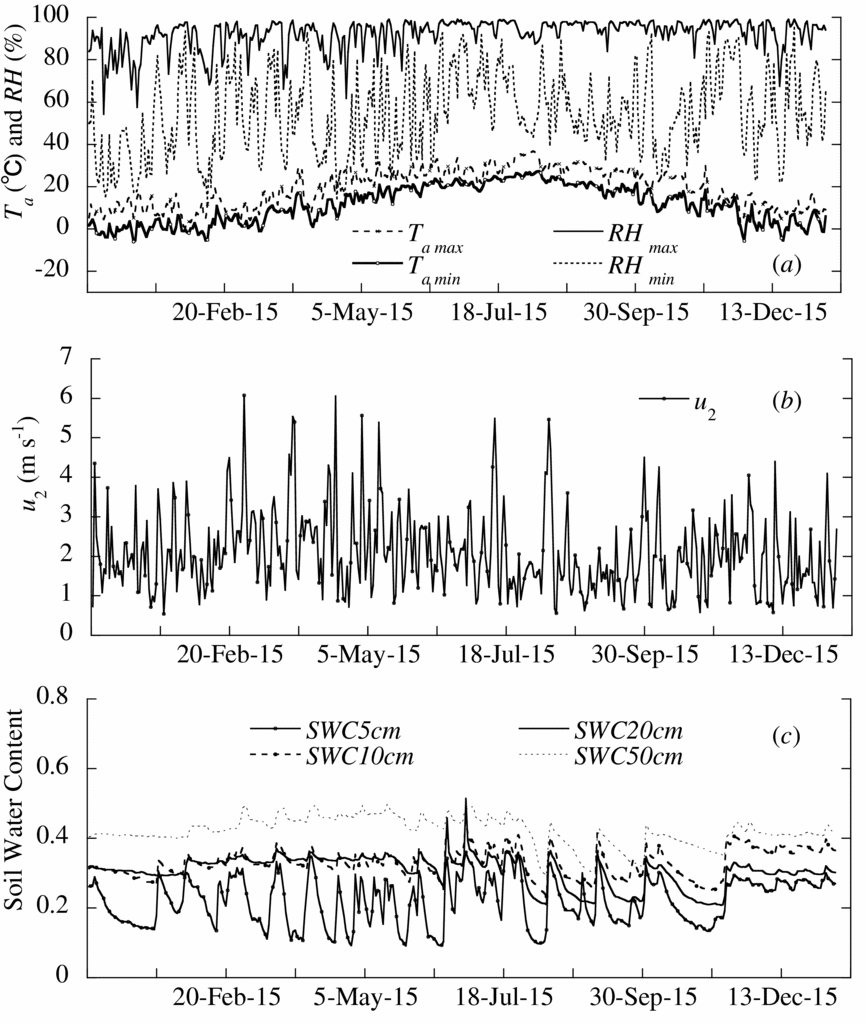
The elements of radiation balance, the global solar radiation (SR), the albedo of the tea field (α), the downward long wave radiation from the atmosphere (Ld) and the upward long wave radiation from the tea field (Ld), were measured with a CNR-4 sensor (Kipp and Zonen, the Netherlands) at 2.5 m and thus the net radiation (Rn = (1 – α) SR + Ld – Lu) was calculated. Here, soil heat flux was measured at 2 cm depth with a soil heat plate HFP01-L10 (Campbell Scientific, USA). Soil water content and soil temperature were measured with Hydra Probe sensors by setting the sensors at five different depths within the soil layer (5, 10, 20, 50 and 70 cm). Vertical profiles (1.5 and 2.0 m above the ground surface) of air temperature (Ta) and relative humidity above the canopy were measured with psychrometers HMP155A (Vaisala, Finland). The accuracy of the psychrometers was validated before the field observation. Wind speed was measured with three three-cup anemometers A100L2 (MetOne, USA) at the same height as Ta. Rainfall was measured with TE525MM (Campbell, USA) at the same field. All the data were sampled every 10 s, averaged every 10 min and recorded by a data logger CR3000-NB (Campbell Scientific, USA). In this study, the direction of the prevailing winds during growing season were westerly, the influence of fetch was not considered due to the similar coverage and irrigation intensity for 200 m of upwind of the observation field. The observed meteorological data are shown in Figure 1. The Bowen ratio energy balance method was used to estimate the hourly latent heat flux of tea field. The canopy height was measured monthly.
The observed meteorological data from 9 Dec. 2014 to 10 Jan. 2016 in a tea field.

Methods
Bowen ratio energy balance method (BREB) and Penman–Monteith model
The Bowen ratio and the energy balance equation are the basis for the method of determining LET using micrometeorological and soil heat flow measurements (Wight et al., Reference Wight, Hanson, Wright, Allen and Van Bavel1993). The energy budget in the tea field is written as
 $$\begin{equation}
{R_n} = LET + H + G
\end{equation}$$
where Rn is the net radiation (W m−2), LET is latent heat flux (W m−2), H is sensible heat flux (W m−2), G is soil heat flux (W m−2). The Bowen ratio (β) is the ratio of sensible heat flux to latent heat flux (H/LET) and can be estimated from the temperature and vapour pressure gradients, β = γΔT/Δe, ΔT is the air temperature gradient, Δe is the vapour pressure gradient and γ is the psychrometric coefficient. LET was obtained based on the heat balance at the canopy surface expressed by the rearranged energy balance equation (Wight et al., Reference Wight, Hanson, Wright, Allen and Van Bavel1993). In this study, the results of LET were neglected when β is close to −1, which occurred at night-time:
 $$\begin{equation}
LET = \frac{{{R_n} - G}}{{1 + \beta }}
\end{equation}$$
LET can also be expressed as (Allen et al., Reference Allen, Pereira, Raes and Smith1998)
 $$\begin{equation}
LET = \frac{{\Delta \left( {{R_n} - G} \right) + \frac{{{\rho _a}{c_p}\left( {{e_s} - {e_a}} \right)}}{{{r_a}}}}}{{\Delta + \gamma \left( {1 + \frac{{{r_c}}}{{{r_a}}}} \right)}}
\end{equation}$$
based on the PM model. Where LET is the latent heat flux density (W m−2), Rn and G are, respectively, the net radiation and soil heat flux (W m−2), Δ is the saturation vapour pressure slope (Pa °C−1), ρa is the mean air density at constant pressure (kg m−3), cp is the specific heat of moist air (J kg °C −1), es and ea are, respectively, the saturation and actual vapour pressure of the air (Pa), γ is the psychrometric coefficient (Pa °C −1), ra is the aerodynamic resistance (s m−1), and rc is the canopy resistance (s m−1). The determination of Δ, ρa and cp was done according to Allen et al. (Reference Allen, Pereira, Raes and Smith1998).
Estimation of resistances
The aerodynamic resistance (ra) can be calculated by the following equation:
 $$\begin{equation}
{r_a} = \frac{1}{{u{k^2}}}\left[ {\ln \left( {\frac{{{z_{{\rm{ref}}}} - d + {z_H}}}{{{z_H}}}} \right) + {\psi _H}} \right] \cdot \left[ {\ln \left( {\frac{{{z_{{\rm{ref}}}} - d + {z_m}}}{{{z_m}}}} \right) + {\psi _m}} \right]
\end{equation}$$
where k is von Karman's constant (=0.41), z ref is the reference height of measurements for both temperature and wind speed (m), u is the mean wind speed (m s−1) at height z ref, d is the zero plane displacement (m), zH is the surface roughness for the heat flux (m), assumed to be equal to roughness length for water vapour, taken to be 0.1zm, zm is the surface roughness for momentum flux (m), ψH and ψm are the atmospheric stability correction factor for the heat flux and momentum flux, respectively, and are functions of (z ref –d)/L (see Brutsaert, Reference Brutsaert1982), where L is the Monin–Obukhov length (m). The parameters d and zm are defined as 0.63 and 0.13 of the canopy height, respectively (Monteith, Reference Monteith1973).
The canopy resistance (rc) computed from the PM model based on the measurements of meteorological conditions and LET can be written as
 $$\begin{equation}
{r_c} = \left[ {\frac{{\Delta \left( {{R_n} - G} \right) + \frac{{{\rho _a}{c_p}\left( {{e_s} - {e_a}} \right)}}{{{r_a}}}}}{{LET}} - \Delta } \right]\frac{{{r_a}}}{\gamma } - {r_a}
\end{equation}$$
One approach for estimating rc, suggested by Katerji and Perrier (Reference Katerji and Perrier1983), was establishing a relationship between two ratios r c/ra and r*/ra. The parameter r* was first introduced by Monteith (Reference Monteith1965) and mainly depends on climatic variables, and is referred to as climatic resistance (Perez et al., Reference Perez, Lecina, Castellvi, Martinez-Cob and Villalobos2006). The derivation of the Katerji and Perrier method is shown below. First, the Eq. (4) can be written as
 $$\begin{equation}
LET = \frac{{\Delta \left( {{R_n} - G} \right)\left[ {1 + \frac{{{\rho _a}{c_p}\left( {{e_s} - {e_a}} \right)}}{{\Delta \left( {{R_n} - G} \right)}} \cdot \frac{1}{{{r_a}}}} \right]}}{{\left( {\Delta + \gamma } \right) + \gamma \frac{{{r_c}}}{{{r_a}}}}}
\end{equation}$$
and can be arranged as
 $$\begin{equation}
LET = \frac{\Delta }{{\Delta + \gamma }}\left( {{R_n} - G} \right)\frac{{1 + \frac{{{\rho _a}{c_p}\left( {{e_s} - {e_a}} \right)}}{{\Delta \left( {{R_n} - G} \right)}} \cdot \frac{1}{{{r_a}}}}}{{1 + \frac{\gamma }{{\Delta + \gamma }} \cdot \frac{{{r_c}}}{{{r_a}}}}}
\end{equation}$$
By defining a climatic resistance given as
 $$\begin{equation}
{r^ * } = \frac{{\Delta + \gamma }}{\gamma }\frac{{{\rho _a}{c_p}\left( {{e_s} - {e_a}} \right)}}{{\Delta \left( {{R_n} - G} \right)}}
\end{equation}$$
So, the Eq. (7) can be rewritten as
 $$\begin{equation}
LET = \frac{\Delta }{{\Delta + \gamma }}\left( {{R_n} - G} \right)\frac{{1 + \frac{\gamma }{{\Delta + \gamma }} \cdot \frac{{{r^ * }}}{{{r_a}}}}}{{1 + \frac{\gamma }{{\Delta + \gamma }} \cdot \frac{{{r_c}}}{{{r_a}}}}}
\end{equation}$$
Katerji and Perrier (Reference Katerji and Perrier1983) presented a linear link between r*/ra and r c/ra. In this study, we found a non-linear functional relationship between r*/ra and r c/ra, which has a higher correlation coefficient than the linear relationship shown in Yan et al. (Reference Yan, Shi, Oue, Zhang, Xue, Cai and Wang2015a):
 $$\begin{equation}
\frac{{{r_c}}}{{{r_a}}} = a \times \frac{{{r^ * }}}{{{r_a}}} + b \times \sqrt {\frac{{{r^ * }}}{{{r_a}}}} + c
\end{equation}$$
where a, b and c were empirically fitted.
The accuracy and applicability of r c estimated by r* (Katerji and Perrier, Reference Katerji and Perrier1983) was assessed by integrating the r c sub-model into the PM model in the present study area, and compared the estimated LET with measured using the Bowen ratio energy balance method with different dataset.
Statistical analysis
The statistical indices root mean square error (RMSE), systematic RMSE (MSEs), unsystematic RMSE (MSEu) and index of agreement (d) were calculated for validating the accuracy of the constructed model as
 $$\begin{equation}
RMSE & =& {\left[ {\frac{1}{n}\sum\limits_{i = 1}^n {{{({P_i} - {M_i})}^2}} } \right]^{1/2}}\\
\end{equation}$$
 $$\begin{equation}
MS{E_s} & =& \left[ {\frac{1}{n}\sum\limits_{i = 1}^n {{{({\hat{P}_i} - {M_i})}^2}} } \right]^{1/2}\\
\end{equation}$$
 $$\begin{equation}
MS{E_u} & =& {\left[ {\frac{1}{n}\sum\limits_{i = 1}^n {{({\hat{P}_i} - {P_i})}^2} } \right]^{1/2}}\\
\end{equation}$$
 $$\begin{equation}
d & =& 1 - \left[ {\frac{{n \cdot RM{S^2}}}{{\sum\limits_{i = 1}^n {\left( {\left( {} \right.\left| {{P_i} - \overline M } \right| + \left| {{M_i} - \overline M } \right|{{\left. {} \right)}^2}} \right)} }}} \right]
\end{equation}$$
RESULTS AND DISCUSSION
Seasonal and diurnal variations of energy budget
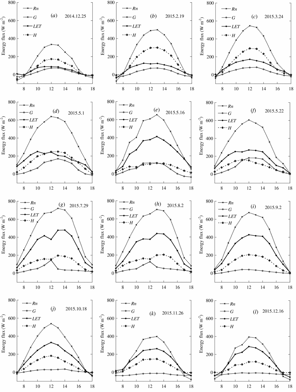
Twelve days in different seasons through the year were selected for analysing the seasonal variation in energy budget measured at a tea field (Figure 2). The maximum net radiation (Rn) increased from 334.4 W m−2 (Dec. 25, 2014) to 703.5 W m−2 (Aug. 2, 2015), and then was decreased to 400 W m−2 at Dec. 16, 2015. The maximum latent heat flux LET was 89.2 W m−2 at Dec. 25, 2014, and then increased to 413.2 W m−2 at May 16, 2015; the maximum LET was 503.9 W m−2 at Jul. 29, 2015, and then decreased to 261.8 W m−2 at Nov. 26, 2015. The average ratio of LET to Rn varied from 41.1% (Feb. 19, 2015, Figure 2b) to 72.8% (Sep. 2, 2015, Figure 2i). The ratio of sensible heat flux (H) to Rn changed when varying the Bowen ratio. The ratio of soil heat flux (G) to Rn was the lowest in the entire energy budget, and the average G ranged from −25.9 to 76.1 W m−2. The Rn, LET and H were positive during 8:00 to 18:00 from May 22 to Oct. 18, 2015, while the values were negative from 17:00 after Oct. 18, 2015.
The energy budget in a tea field in different season through the year, Rn is the net radiation (W m−2), LET is latent heat flux (W m−2), H is sensible heat flux (W m−2) and G is soil heat flux (W m−2).

Seasonal and diurnal variation of canopy and aerodynamic resistance
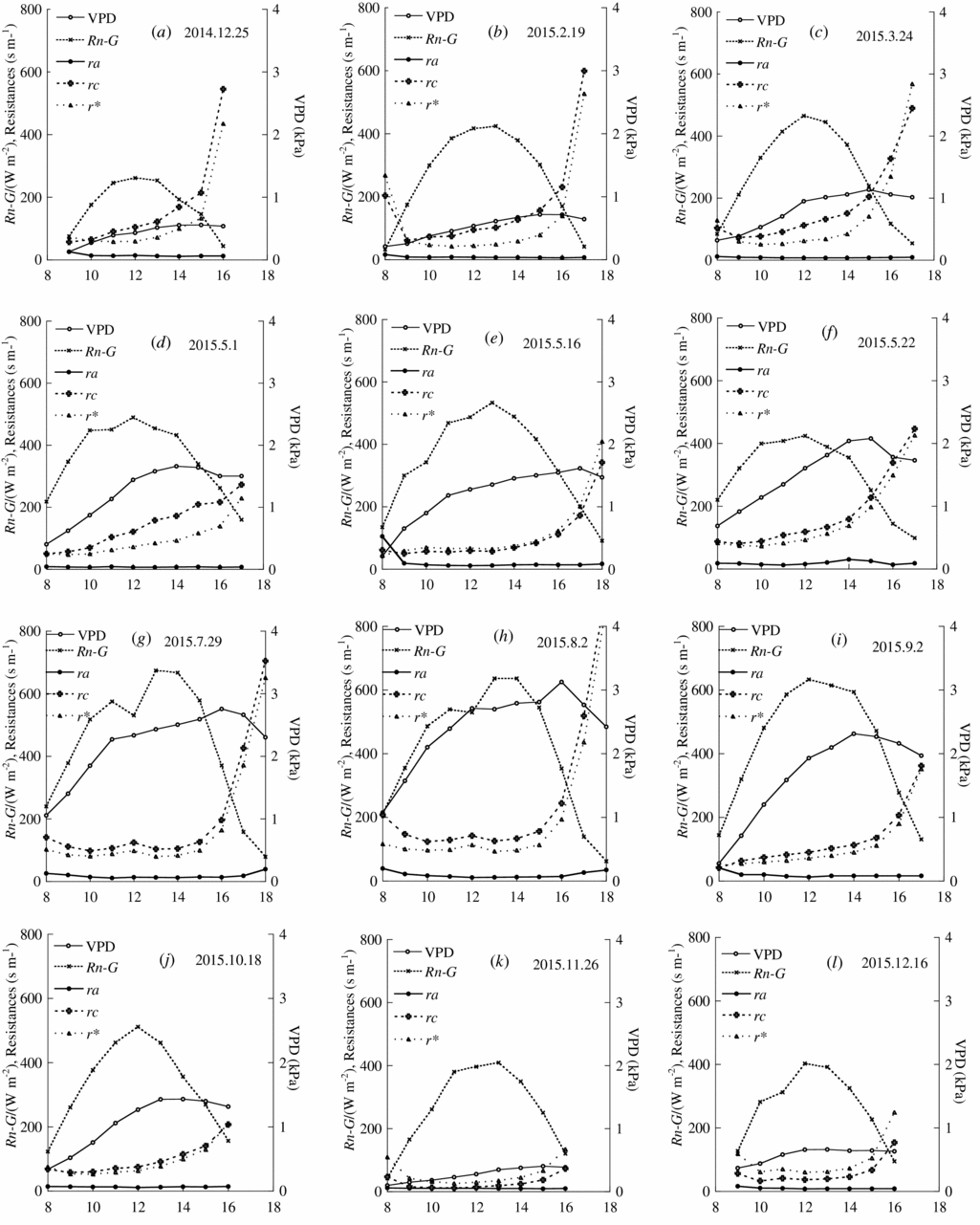
The hourly evolution of rc computed by inverting the PM equation with the hourly measured LET. The hourly variations of ra, r*, VPD and net radiation were shown together with rc in Figure 3. In order to show the variations of rc and ra in different seasons through the years, data at Dec. 25, 2014, Feb. 19, Mar. 24, May 1, May 16, May 22, Jul. 29, Aug. 2, Sep. 2, Oct. 18, Nov. 26 and Dec.16, 2015 were chosen for analysis. Among these days, the maximum values of VPD ranged from 0.40 to 3.13 kPa and happened at 14:00 for most of days. The VPD were higher from May to September, while the values were relative low in November to March. The daytime variation of rc is characterized by high values in afternoon (from 16:00), low and relative constant values between 10:00 to 15:00 and the value is higher in afternoon than in the morning at same net radiation condition. The rc increases to extremely larger values (> 2000 s m−1) after 18:00. For the whole year, rc shows high values in summer season (May 22, Jul. 29, Aug. 2), while low values in winter season (Nov. 26 and Dec.16, 2015). Those results indicate that cool and relative high wind speed blow away the water vapour layer at the leaf surface and replace it by relative low humidity of the air, lowering rc and increasing transpiration. On the other hand, strong winds may cause stomatal closure, increasing rc and reducing transpiration. The values of ra estimated by the classical logarithmic profile equations were very low for all seasons; most data were lower than 100 s m−1. This is likely due to the low plant coverage of the tea field and relative high wind speed. Yan et al. (Reference Yan, Shi, Oue, Zhang, Xue, Cai and Wang2015a) presented similar variation but higher value of ra for buckwheat and maize. The values of r* showed a negative variation with Rn and increased drastically after 15:00 because of the decrease in Rn (Figure 3).

Parameterization of rc
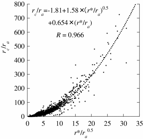
Yan et al. (Reference Yan, Zhang, Oue, Wang and He2015a) presented non-linear relationships for parameterization of rc for maize and buckwheat based on same data for model calibration and validation. Herein, similar non-linear relationship was calibrated for modelling rc for tea plants based on the data from different seasons and years. Figure 4 shows the diurnal variation of experimental values of rc/ra versus r*/ra in tea field, with a quadratic polynomial relationship being found between rc/ra and (r*/ra) 0.5. The regression curves between rc/ra and r*/ra for tea crop obtained in this study was similar to the result presented by other researchers for different crops. However, the coefficients a, b and c in Eq. (10) were different from the values reported in other studies (He et al., Reference He, Oue and Oki2009: wheat field, 0.88, 0.82 and –1.95; Yan et al., Reference Yan, Shi, Oue, Zhang, Xue, Cai and Wang2015a: buckwheat field, 0.73, 1.25 and −0.28, and maize field, 3.09, 2.41and 0.62). Katerji et al. (Reference Katerji, Rana and Fahed2011) calibrated a linear relationship between rc/ra and r*/ra on grass with R equal to 0.77 based on the data of 2 days; they pointed out that the slopes, the intercepts and the correlation coefficients obtained by linear regression analysis varied for each species. The linear relationships between rc/ra and r*/ra observed on soybean, sweet sorghum and vineyard by Katerji and Rana (Reference Katerji and Rana2006; Reference Katerji and Rana2008) showed better correlation coefficients with values of 0.69, 0.92 and 0.78, respectively. As pointed out by Rana et al. (Reference Rana, Katerji, Mastorilli, EI Moujabber and Brisson1997), the coefficients of those relationships depend on the type of crop, its phenological state or soil water status. Even for the same crop, the differences in coefficients among studies may exist when different diurnal periods are considered. Based on our results, which are in agreement with Perez et al. (Reference Perez, Lecina, Castellvi, Martinez-Cob and Villalobos2006), the best fit corresponded to a dependence of rc/ra on the square root of r*/ra (Figure 4).
The diurnal variation of experimental values of rc/ra versus r*/ra in a tea field.

Calculation of hourly LET by the PM equation with rc sub-model
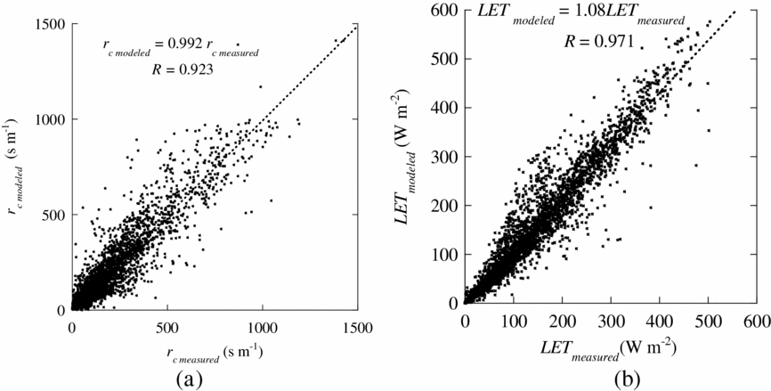
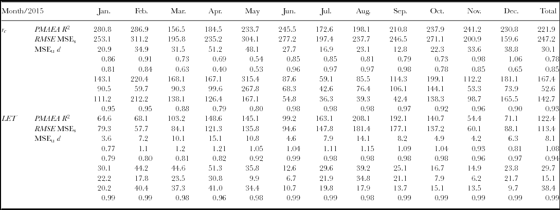
The hourly LET of a tea field could be estimated with the PM model using rc sub-models. The comparisons between measured and modelled rc and LET for tea plants are shown in Figure 5. Data for the days used to calibrate the rc sub-model were not used for comparison between measured and modelled rc and LET. The daytime (8:00-18:00) variations of rc and LET for tea are shown and good agreements between measured and modelled rc and LET were found. The average absolute errors between measured rc and LET were 30.1 s m−1 and 8.1 W m−2. As shown in Figure 5, there were high correlations between measured and estimated rc and LET. The regression points for both rc and LET were scattered close to 1:1 line with some exceptions. This means the estimated rc and LET values were close to the measured values. The monthly slope values are in the range 0.54–1.06, and 0.77–1.21 between measured and modelled rc and LET, respectively. The coefficients of determination (R 2) were 0.85 and 0.94 for rc and LET, respectively. The other statistical parameters, such as systematic mean square errors (MSEs), unsystematic mean square errors (MSEu) and index of agreement (d) are shown in Table 1, together with the monthly average rc and LET. The results showed that both rc and LET could be estimated with relatively high accuracy. The highest values of R 2 for estimating rc and LET happened during June to October. Relative low values of RMSE were obtained during June to November. It might because that the rc values increased to over 1000 s m−1 earlier in the late afternoon in winter and spring seasons (around 16:00) than in the summer season (around 18:00), while high rc always lead to the divergence of LET. The two-tail t-test statistical analysis showed there were no significant differences between measured and estimated rc and LET. However, the resulting coefficients for Eq. (15) in the present study still need validation if the model is used in other climatic conditions. In this study, we modelled hourly rc and LET as there was significant variation of rc after 16:00 (as shown in Figure 3). In fact, modelling of LET using hourly time steps of rc is more reasonable than using daily time steps as the daily average for rc may not reflect the real variation of rc, misrepresent LET and introduce error into the calculation (Allen et al., Reference Allen, Pereira, Raes and Smith1998). On the other hand, modelling hourly rc and LET can improve our understanding of leaf stomatal status and total energy partitioning during the day. Hence, modelling rc and LET based on hourly scale data was more reasonable and reliable than modelling based on daily data.
The comparison between measured and modelled (a) rc and (b) LET.

Error analysis statistics of the comparison between measured and estimated rc and LET for tea plants.

*P and M are mean estimated and measured rc (s m−1) and LET (w m−2), respectively; AE is absolute error (w m−2); a is slope of least square regression line, R 2 coefficients of determination, RMSE root mean square error (w m−2), MSEs systematic mean square error (w m−2), MSEu unsystematic mean square error (w m−2), d index of agreement; a, R 2 and d are dimensionless.
CONCLUSION
A simple rc sub-model was constructed based on the climatic date in a tea field to predict the LET for different seasons of tea plants. The rc was parameterized by a climatic resistance r*, the rc sub-model was integrated into the PM model for predicting hourly LET and the accuracy was compared with measured LET by Bowen ratio energy balance method. The monthly accuracy of constructed model was analysed and we concluded that the PM model provided good estimates of measured LET of tea field with constructed rc sub-model for different seasons.
Acknowledgements
We greatly appreciate the careful and precise reviews by the anonymous reviewers and editors. This study has been financially supported by the Natural Science Foundation of China (51509107,51609103), the Key Laboratory of Agricultural Water Resources, the Chinese Academy of Sciences (No. KFKT201605), Natural Science Foundation of Jiangsu province (BK20140546, BK20150509), the Scientific Research Foundation for the Returned Overseas Chinese Scholars, State Education Ministry (2015, No. 311) and Jiangsu University senior professional scientific research fund project (14JDG015, 14JDG017, 12JDG097).